Differential quadrature method for space-fractional diffusion equations on 2D irregular domains

Abstract

In mathematical physics, the space-fractional diffusion equations are of particular interest in the studies of physical phenomena modelled by Lévy processes, which are sometimes called super-diffusion equations. In this article, we develop the differential quadrature (DQ) methods for solving the 2D space-fractional diffusion equations on irregular domains. The methods in presence reduce the original equation into a set of ordinary differential equations (ODEs) by introducing valid DQ formulations to fractional directional derivatives based on the functional values at scattered nodal points on problem domain. The required weighted coefficients are calculated by using radial basis functions (RBFs) as trial functions, and the resultant ODEs are discretized by the Crank-Nicolson scheme. The main advantages of our methods lie in their flexibility and applicability to arbitrary domains. A series of illustrated examples are finally provided to support these points.

1 Introduction

During recent decades, a bulk of attention has been attracted to a special part of partial differential equations (PDEs), i.e., the so-called fractional PDEs, especially those abstracted from practical problems. As a new class of mathematical models, fractional PDEs show good promise in characterizing the physical processes with memory effort and historical dependence, such as the anomalous dispersion in complex heterogeneous aquifer and fractal geometry Ref02 ; Ref03 , thereby making up for the defect of inconsistency with the reality when an integer-order model is applied to describe the similar non-classical phenomena. The relevant applications include crystal dislocation, hydrodynamics, electrochemistry, plasma turbulence, continuum mechanics, and so forth Ref10 ; Ref08 ; Ref11 ; Ref12 ; Ref09 . There is still a rapidly growing interest on these subjects in this moment. Due to the universal mutuality, however, their solutions can rarely be represented by elementary functions in closed forms. A few existent analytic solutions are limited to very simple cases or achieved in series or integral forms under theoretical restrictions; see R28 ; R27 ; R25 ; R26 and references therein. This presents a severe challenge for developing sufficiently valid analytic techniques for these equations, so numerical algorithms have been favored and gradually emerged as essential alternatives in actual investigation.

The space-fractional PDEs constitute an important branch of PDEs in the studies on the evolution of complex dynamic behavior governed by Lévy flights. As compared to the time-fractional PDEs, seeking the approximate solutions to such equations appears to be more difficult by virtue of the vector structure of fractional Laplacian. Up to date, various numerical algorithms have been designed, covering finite difference methods Ref15 ; Ref14 ; R05 ; R07 ; R08 ; Ref13 , general Padé approximation R04 , meshless point interpolation methods R09 ; R10 , moving least-squares meshless method xz01 , finite element methods Ref16 ; R12 , discontinuous Galerkin method (DGM) R14 , finite volume methods R15 ; R16 , spline approximation method (SAM) R17 , and spectral collocation methods Ref17 ; R18 ; R20 . In R24 ; R21 ; R23 ; R22 , a series of operational matrix methods were constructed based on the approximate expansions by using shifted Jacobi, Chebyshev, Legendre polynomials, and Haar wavelets functions, as elements, respectively. In Ref18 , a Crank–Nicolson alternative direction implicit Legendre-Galerkin spectral method has been derived for nonlinear 2D Riesz space-fractional reaction-diffusion equations. Du and Wang developed a finite element method (FEM) conjectured with a fast algebraic solver for the steady space-fractional diffusion equations by dividing the unit square domain into quadrilateral meshes Ref07 . It is noteworthy that, nevertheless, all of the mentioned algorithms are only available for one-dimensional or rectangular domain problems. Few works go for a valid method for the fractional problems on irregular domains. Liu et. al handled a 2D fractional FitzHugh-Nagumo monodomain model by an implicit semi-alternative direction difference scheme on circular domain and a union of half-circular and half-square domains with square meshes Ref06 , where the outer peripheral nodal points are in an approximate match for boundaries. In Ref01 , we proposed a fully discrete FEM for space-fractional Fisher’s equation on rectangular domains and the generated meshes are relaxed to be unstructured; later, it has been extended to the space-fractional diffusion equations on polygonal and elliptic domains Ref04 . Qiu et al. developed a nodal DGM for the same type equations on unstructured triangular meshes and a L-shaped domain problem was considered Ref05 . Pang et al. applied the RBFs meshless collocation methods to solve the 2D space-fractional advection-diffusion equations on polygonal and circular domains xz04 . In general, finite difference method (FDM) is implemented on pre-defined meshes and inherits the shortcomings including the difficulty in simulation of complex domain problems. DGM, FEM alleviate this issue, but both of them hinge on variational principles and suffer huge computational burden and inflexibility to calculate the entities of their stiffness matrices that are on longer sparse.

Recent years have witnessed a keen interest in meshless techniques, which avoid troublesome mesh generation and reconstruction, or only use easily generable meshes in a flexible manner. The meshless methods are superior to convectional mesh-dependent methods in terms of simulating complex flow, structure destruction, and extremely large deformation problems, because they eliminate the element connectivity data and build trial functions entirely on scattered nodal points to decretize these problems. Being a promising direction in computational mechanics, various meshless methods have been reported for numerical solutions of PDEs, typically including smooth particle hydrodynamics xz05 , finite point method xz06 , reproducing kernel particle method xz08 , partition of unity method xz13 , diffuse element method xz10 , finite sphere method, element-free Galerkin methods xz02 ; xz03 , meshless local Petrov-Galerkin method xz09 , boundary node method, point interpolation method xz14 , and the others. We refer the readers to xz12 ; xz11 for their overall views.

DQ method is understood as a direct numerical approach for finding the solutions of PDEs by reducing the equations into ODEs via approximating the space derivatives as the weighted linear sums of the functional values at finite nodal points on problem domains. It was pioneered by Bellman and Casti R30 , and further discussed based on different basis functions, such as Lagrangian interpolation basis functions, RBFs, orthogonal polynomials, Sinc and spline basis functions Ref20 ; Ref19 ; R37 ; R39 ; R36 . DQ method can achieve high accuracy by using a few nodal points; besides, it is straight forward to implement and truly meshless. In this context, regarding the current interest in fractional PDEs as effective models, we attempt to establish valid DQ methods to solve the 2D space-fractional diffusion equations on arbitrary domains. The Multiquadric, Inverse Multiquadric, and Gaussian RBFs are utilized as trial functions to determine the weighted coefficients that we require to evaluate the fractional directional derivatives as the weighted linear sums of the functional values at regularly distributed or scattered nodal points on problem domains; the Crank-Nicolson scheme is employed to advance the solutions in time. The proposed methods extend the traditional DQ methods while inheriting their principal features. The convergent behaviors of these techniques are studied on several numerical benchmarks with a varying nodal number, including the square, trapezoidal, circular, and L-shaped domain problems.

The skeleton is organized as follows. In Section 2, the space-fractional diffusion equations on a 2D domain are introduced for preliminaries. Section 3 studies the DQ formulations for fractional directional derivatives and the way to determine their weights by means of RBFs. In Section 4, we construct time-stepping DQ methods by using the Crank-Nicolson scheme in time and show the details of implementation. In Section 5, illustrative tests on regular and irregular domains are carried out to examine their accuracy and effectiveness. A concise remark is finally drawn in the last section.

2 Model problems

On a bounded domain $\Omega\subset\mathbb{R}^{2}$ with its boundary being $\partial\Omega$, the continuous 2D space-fractional diffusion equations are as follows

$$\frac{\partial u(x,y,t)}{\partial t}-\kappa\!\int_{0}^{2\pi}\mathcal{D}^{\alpha}_{\theta}u(x,y,t)P(\theta)d\theta\!=\!f(x,y,t),\ (x,y;t)\in\Omega\times(0,T],$$ (1)

subjected to the initial and boundary conditions

$$u(x,y,0)=u_{0}(x,y),\quad(x,y)\in\Omega,$$ (2)

$$u(x,y,t)=g(x,y,t),\quad(x,y;t)\in\mathbb{R}^{2}\backslash\Omega\times(0,T],$$ (3)

where $1<\alpha\leqslant 2$, $\kappa$ is the non-negative diffusivity parameter, $P(\theta)d\theta$ is a probability measure on the unit disk of $\mathbb{R}^{2}$, and $f(x,y,t)$ is the pre-prescribed source function. In Eq. (1), $\mathcal{D}^{\alpha}_{\theta}u(x,y,t)$ stands for the space-fractional directional derivatives defined in Caputo sense, i.e.,

$$\mathcal{D}^{\alpha}_{\theta}u(x,y,t)=\mathcal{I}^{2-\alpha}_{\theta}\mathcal{D}^{2}_{\theta}u(x,y,t),\quad 0\leqslant\theta<2\pi,$$ (4)

with the integer-order directional derivatives

$$\mathcal{D}^{m}_{\theta}v(x,y)=\bigg{(}\cos\theta\frac{\partial}{\partial x}+\sin\theta\frac{\partial}{\partial y}\bigg{)}^{m}v(x,y),\quad m\in\mathbb{N},$$

and the fractional directional integration

$$\mathcal{I}^{\mu}_{\theta}v(x,y)=\frac{1}{\Gamma(\mu)}\int_{0}^{z(x,y,\theta)}\omega^{\mu-1}v(x-\omega\cos\theta,y-\omega\sin\theta)d\omega,$$

for $\mu>0$ while $\mathcal{I}^{\mu}_{\theta}v(x,y)=v(x,y)$ for $\mu=0$. $z(x,y,\theta)$ denotes the distance from the nodal point $(x,y)$ to $\partial\Omega$ in the direction $(-\cos\theta,-\sin\theta)$; see Fig. 1. In particular, when $\theta$ is taken to be some special values as $0$, $\pi$, $\mathcal{D}^{\alpha}_{\theta}u(x,y,t)$ recovers to the commonly used Caputo derivatives with regard to $x$ Ref09 , i.e.,

$$\mathcal{D}^{\alpha}_{0}u(x,y,t) =\frac{1}{\Gamma(2-\alpha)}\int^{x}_{\Gamma_{1}(x,y)}\frac{\partial^{2}u(\omega,y,t)}{\partial\omega^{2}}\frac{d\omega}{(x-\omega)^{\alpha-1}},$$ (5)

$$\mathcal{D}^{\alpha}_{\pi}u(x,y,t) =\frac{1}{\Gamma(2-\alpha)}\int^{\Gamma_{2}(x,y)}_{x}\frac{\partial^{2}u(\omega,y,t)}{\partial\omega^{2}}\frac{d\omega}{(\omega-x)^{\alpha-1}},$$ (6)

and Eqs. (1)-(3) degenerate into the space-fractional diffusion equations in coordinate forms, which have been the topics of intense research, where $\Gamma_{1}(x,y)$, $\Gamma_{2}(x,y)$ are the subsets of $\partial\Omega$, and satisfy $\partial\Omega=\Gamma_{1}(x,y)\cup\Gamma_{2}(x,y)$ and $\Gamma_{1}(x,y)\cap\Gamma_{2}(x,y)=\varnothing$, for which, $A$, $B$ are dividing points; see Fig. 1.

In the sequel, without loss of generality, we consider the multi-term 2D space-fractional diffusion equations with variable coefficients

$$\frac{\partial u(x,y,t)}{\partial t}-\sum_{l=1}^{L}\kappa_{l}(x,y)\mathcal{D}^{\alpha_{l}}_{\theta_{l}}u(x,y,t)=f(x,y,t),\ \ (x,y;t)\in\Omega\times(0,T],$$ (7)

subjected to the initial and boundary conditions

$$u(x,y,0)=u_{0}(x,y),\quad(x,y)\in\Omega,$$ (8)

$$u(x,y,t)=g(x,y,t),\quad(x,y;t)\in\mathbb{R}^{2}\backslash\Omega\times(0,T],$$ (9)

where $1<\alpha_{l}\leqslant 2$, $0\leqslant\theta_{l}<2\pi$, $L\in\mathbb{Z}^{+}$, $\kappa_{l}(x,y)$ are the non-negative diffusivity parameters but do not fulfill $\sum_{l=1}^{L}\kappa_{l}(x,y)\equiv 0$, and $\mathcal{D}^{\alpha_{l}}_{\theta_{l}}u(x,y,t)$ are the Caputo directional derivatives. Due to the characteristics of Lévy processes, the boundary constrains of space-fractional diffusion equations as Eqs. (1), (7) should be specified on the complementary set of $\Omega$ xz16 , so that model problems can be well-posed. In this context, we assume that (9) is always homogeneous outside $\Omega$, but may not be homogeneous at its boundary, which says that the diffusive particles are killed after they escape from $\Omega$.

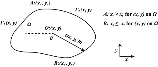
Figure 1: The subsets of boundary $\Gamma_{1}(x,y)$, $\Gamma_{2}(x,y)$ and the distance $z(x,y,\theta)$ of $(x,y)$.

3 DQ approximations for fractional directional derivatives

In this section, we derive valid DQ formulations for approximating the fractional directional derivatives and study how to compute the weighted coefficients by using Multiquadric, Inverse Multiquadric, and Gaussian RBFs as trial functions. To start with, let $\Omega\subset\mathbb{R}^{2}$ be a bounded domain and $\textbf{x}_{i}$, $i=0,1,\ldots,M$, be a sequence of scattered nodal points distributed on $\Omega$ with $\textbf{x}_{i}=(x_{i},y_{i})$. Define a set of proper basis functions $\{\phi_{k}(\textbf{x})\}_{k=0}^{M}$ that are adequately smooth to guarantee the existence of fractional directional derivatives. DQ formulation can be described as combining evaluations of a function at finite nodal points on problem domain so as to get a direct approximation to its partial derivative with regard to a variable. In general, we always interpolate the exact solution of a fractional PDE like Eqs. (1)-(3) in the form

$$u(\textbf{x},t)\cong\sum_{k=0}^{M}\delta_{k}(t)\phi_{k}(\textbf{x}),$$ (10)

then enforce it to satisfy main equation as well as the related restrictions at collocation points to determine the unknowns $\{\delta_{k}(t)\}_{k=0}^{M}$. However, if we have

$$\mathcal{D}^{\alpha}_{\theta}\phi_{k}(\textbf{x}_{i})=\sum\limits_{j=0}^{M}{\omega_{ij}^{(\alpha)}\phi_{k}(\textbf{x}_{j})},\ \ i,k=0,1,\ldots M,$$ (11)

and substitute Eq. (11) into Eq. (10) after acting the differential-integral operator $\mathcal{D}^{\alpha}_{\theta}$ on both sides of Eq. (10), it suffices to show that

$$\mathcal{D}^{\alpha}_{\theta}u(\textbf{x}_{i},t)\cong\sum_{k=0}^{M}\delta_{k}(t)\mathcal{D}^{\alpha}_{\theta}\phi_{k}(\textbf{x}_{i})=\sum_{k=0}^{M}\delta_{k}(t)\sum\limits_{j=0}^{M}{\omega_{ij}^{(\alpha)}\phi_{k}(\textbf{x}_{j})}\cong\sum\limits_{j=0}^{M}{\omega_{ij}^{(\alpha)}u(\textbf{x}_{j},t)},$$ (12)

in the light of the linearity of $\mathcal{D}^{\alpha}_{\theta}$. In other words, Eqs. (12) are valid DQ approximations to $\mathcal{D}^{\alpha}_{\theta}u(\textbf{x}_{i},t)$, $i=0,1,\ldots,M$, as long as Eqs. (11) are fulfilled. As a result, an approximate solution of a fractional PDE can be found by solving a set of ODEs without knowing $\{\delta_{k}(t)\}_{k=0}^{M}$. We term $\omega_{ij}^{(\alpha)}$, $i,j=0,1,\ldots,M$, by the weighted or DQ coefficients for fractional directional derivatives, which can be computed via Eqs. (11) by reforming them in matrix-vector forms a priori; $\{\phi_{k}(\textbf{x})\}_{k=0}^{M}$ are referred to as trial or test functions that can typically be chosen by those basis functions mentioned before. When $\alpha\in\mathbb{Z}^{+}$ and $\theta=0$, $\pi$, Eqs. (12) reduce into the DQ formulations for classical derivatives.

3.1 Radial basis functions

The RBFs are known as a family of spline functions which are constructed from the distance between an arbitrary nodal point x and its center $\textbf{x}_{k}$, i.e., $\varphi(||\textbf{x}-\textbf{x}_{k}||)$, abbreviated to $\varphi_{k}(\textbf{x})$, with the Euclidean norm $||\cdot||$. These types of functions provide a set of excellent interpolating bases to interpolate the multivariable scattered data on high-dimensional domains and have been served as an efficient tool in setting up truly meshless numerical algorithms for PDEs by virtue of their independency on geometric complexity and the potential spectral accuracy of their interpolations. Among multiple types of RBFs, three familiar kinds of RBFs will be focused on hereinafter, i.e.,

• Multiquadric RBFs: $\varphi_{k}(\textbf{x})=\sqrt{||\textbf{x}-\textbf{x}_{k}||^{2}+\epsilon^{2}}$,

• Inverse Multiquadric RBFs: $\varphi_{k}(\textbf{x})=\frac{1}{\sqrt{||\textbf{x}-\textbf{x}_{k}||^{2}+\epsilon^{2}}}$,

• Gaussian RBFs: $\varphi_{k}(\textbf{x})=\exp(-\epsilon^{2}||\textbf{x}-\textbf{x}_{k}||^{2})$,

where $k=0,1,\ldots,M$, $M\in\mathbb{Z}^{+}$, and $\epsilon$ is a user number called by shape parameter. Given a function $y(\textbf{x},t)$ defined on $\Omega\subset\mathbb{R}^{d}$, $d=1,2,3$, its interpolating approximation based on these trial bases can be written as

$$y(\textbf{x},t)\cong\sum_{k=0}^{M}\lambda_{k}(t)\varphi_{k}(\textbf{x})+\sum_{s=1}^{M^{*}}\lambda_{M+s}(t)p_{s}(\textbf{x}),$$ (13)

with the unknowns $\{\lambda_{k}(t)\}_{k=0}^{M}$, $\{\lambda_{M+s}(t)\}_{s=1}^{M^{*}}$ yet to be determined by collocating Eq. (13) at nodal points $\{\textbf{x}_{i}\}_{i=0}^{M}$. In order to make the generated algebraic system to be well-posed, the orthogonal conditions

$$\sum_{k=0}^{M}\lambda_{k}(t)p_{s}(\textbf{x}_{k})=0,\quad M^{*}=\frac{(r+d-1)!}{d!(r-1)!},$$ (14)

for $s=1,2,\ldots,M^{*}$, should be imposed, in which, $\{p_{s}(\textbf{x})\}_{s=1}^{M^{*}}$ denote the basis functions of the polynomial space of degree at most $r-1$ on $\mathbb{R}^{d}$. It is worthy to note that the shape parameter $\epsilon$ should be properly assigned in practical computation because it has a significant impact on the approximate power of the radial basis interpolation, so is a RBFs-based method.

3.2 Determination of weighted coefficients

Before proceeding, we notice that the aforementioned polynomials in the right side of Eq. (13) are not always necessary since the augmented interpolating matrix is strictly positive definite for Inverse Multiquadrics, Gaussians, and is conditionally positive definite for Multiquadrics under $M^{*}\geqslant 1$ Ref28 . Hence, for ease of computing the weighted coefficients, we take $M^{*}=0$ for Inverse Multiquadrics, Gaussians, and $M^{*}=1$ for Multiquadrics, in which case, the solvability of the algebraic problem resulting from Eqs. (13)-(14) is guaranteed. For Inverse Multiquadrics and Gaussians, the approximate solution can be expressed by $u(\textbf{x},t)\cong\sum_{k=0}^{M}\lambda_{k}(t)\varphi_{k}(\textbf{x})$. According to Eqs. (10)-(12), we then know the identity related to the fractional operator $\mathcal{D}^{\alpha}_{\theta}$, i.e.,

$$\mathcal{D}^{\alpha}_{\theta}\varphi_{k}(\textbf{x}_{i})=\sum\limits_{j=0}^{M}{\omega_{ij}^{(\alpha)}\varphi_{k}(\textbf{x}_{j})},\ \ i,k=0,1,\ldots M,$$

obtained by directly replacing $\phi_{k}(\textbf{x})$ by $\varphi_{k}(\textbf{x})$ in Eqs. (11), which further lead to the below solvable matrix-vector system:

$$\left(\begin{array}[]{cccc}\varphi_{0}(\textbf{x}_{0})&\varphi_{0}(\textbf{x}_{1})&\cdots&\varphi_{0}(\textbf{x}_{M})\\ \varphi_{1}(\textbf{x}_{0})&\varphi_{1}(\textbf{x}_{1})&\cdots&\varphi_{1}(\textbf{x}_{M})\\ \vdots&\vdots&\ddots&\vdots\\ \varphi_{M}(\textbf{x}_{0})&\varphi_{M}(\textbf{x}_{1})&\cdots&\varphi_{M}(\textbf{x}_{M})\end{array}\right)\left(\begin{array}[]{c}\omega^{(\alpha)}_{i0}\\ \omega^{(\alpha)}_{i1}\\ \vdots\\ \omega^{(\alpha)}_{iM}\end{array}\right)=\left(\begin{array}[]{c}\mathcal{D}_{\theta}^{\alpha}\varphi_{0}(\textbf{x}_{i})\\ \mathcal{D}_{\theta}^{\alpha}\varphi_{1}(\textbf{x}_{i})\\ \vdots\\ \mathcal{D}_{\theta}^{\alpha}\varphi_{M}(\textbf{x}_{i})\end{array}\right),$$ (27)

with $i=0,1,\ldots M$ and the coefficient matrix being fully positive definite. As for Multiquadrics, the polynomial term must be retained so as to ensure the well-posedness of the algebraic problems. Remembering that $M^{*}=1$, there hold $u(\textbf{x},t)\cong\sum_{k=0}^{M}\lambda_{k}(t)\varphi_{k}(\textbf{x})+\lambda_{M+1}(t)$ and the additional condition $\sum_{k=0}^{M}\lambda_{k}(t)=0$. Integrate these two equations into a unified formula to get

$$u(\textbf{x},t)\cong\sum_{k=1}^{M}\lambda_{k}(t)[\varphi_{k}(\textbf{x})-\varphi_{0}(\textbf{x})]+\lambda_{M+1}(t).$$

According to Eqs. (10)-(12), one then has

$$\mathcal{D}^{\alpha}_{\theta}[\varphi_{k}(\textbf{x}_{i})-\varphi_{0}(\textbf{x}_{i})]=\sum_{j=0}^{M}\omega_{ij}^{(\alpha)}[\varphi_{k}(\textbf{x}_{j})-\varphi_{0}(\textbf{x}_{j})],\ \ i=0,1,\ldots M,$$ (28)

for $k=1,2,\ldots,M$, while for $k=0$, it suffices to show

$$\sum_{j=0}^{M}\omega_{ij}^{(\alpha)}=0,$$ (29)

owing to $\mathcal{D}^{\alpha}_{\theta}C=0$ with a constant $C$. Rearranging Eqs. (28)-(29) in matrix-vector forms, a series of linear system of equations are finally obtained:

$$\textbf{A}\boldsymbol{\omega}^{(\alpha)}_{i}=\textbf{D}_{\theta}^{\alpha}\boldsymbol{\varphi}(\textbf{x}_{i})-\textbf{D}_{\theta}^{\alpha}\boldsymbol{\varphi}_{0}(\textbf{x}_{i}),\quad i=0,1,\ldots,M,$$ (30)

where

$$\textbf{A}=\left(\begin{array}[]{cccc}1&1&\cdots&1\\ \varphi_{1}(\textbf{x}_{0})-\varphi_{0}(\textbf{x}_{0})&\varphi_{1}(\textbf{x}_{1})-\varphi_{0}(\textbf{x}_{1})&\cdots&\varphi_{1}(\textbf{x}_{M})-\varphi_{0}(\textbf{x}_{M})\\ \vdots&\vdots&\ddots&\vdots\\ \varphi_{M}(\textbf{x}_{0})-\varphi_{0}(\textbf{x}_{0})&\varphi_{M}(\textbf{x}_{1})-\varphi_{0}(\textbf{x}_{1})&\cdots&\varphi_{M}(\textbf{x}_{M})-\varphi_{0}(\textbf{x}_{M})\end{array}\right),$$

$$\boldsymbol{\omega}^{(\alpha)}_{i}=\left(\begin{array}[]{c}\omega^{(\alpha)}_{i0}\\ \omega^{(\alpha)}_{i1}\\ \vdots\\ \omega^{(\alpha)}_{iM}\end{array}\right),\ \textbf{D}_{\theta}^{\alpha}\boldsymbol{\varphi}(\textbf{x}_{i})=\left(\begin{array}[]{c}\mathcal{D}_{\theta}^{\alpha}\varphi_{0}(\textbf{x}_{i})\\ \mathcal{D}_{\theta}^{\alpha}\varphi_{1}(\textbf{x}_{i})\\ \vdots\\ \mathcal{D}_{\theta}^{\alpha}\varphi_{M}(\textbf{x}_{i})\end{array}\right),\ \textbf{D}_{\theta}^{\alpha}\boldsymbol{\varphi}_{0}(\textbf{x}_{i})=\left(\begin{array}[]{c}\mathcal{D}_{\theta}^{\alpha}\varphi_{0}(\textbf{x}_{i})\\ \mathcal{D}_{\theta}^{\alpha}\varphi_{0}(\textbf{x}_{i})\\ \vdots\\ \mathcal{D}_{\theta}^{\alpha}\varphi_{0}(\textbf{x}_{i})\end{array}\right).$$

The unknown $\boldsymbol{\omega}^{(\alpha)}_{i}$, $i=0,1,\ldots,M$, are the weighted vectors what we seek for. However, here arises another question of how to compute each component of the right-hand vectors $\textbf{D}_{\theta}^{\alpha}\boldsymbol{\varphi}(\textbf{x}_{i})$, $\textbf{D}_{\theta}^{\alpha}\boldsymbol{\varphi}_{0}(\textbf{x}_{i})$, which are the keys to formulating Eqs. (27), (30). Generally, the explicit expressions for the fractional derivatives of a function can be derived but limited to a very small part of functions, that is to say, the explicit expressions are unavailable in most cases, hence the explicit formulas should not be anticipated here, neither are the conventional numerical quadrature rules since the weakly singular integral kernels in fractional derivatives. In the sequel, we evaluate the fractional directional derivatives $\textbf{D}_{\theta}^{\alpha}\boldsymbol{\varphi}(\textbf{x}_{i})$, $\textbf{D}_{\theta}^{\alpha}\boldsymbol{\varphi}_{0}(\textbf{x}_{i})$ by using Gauss-Jacobi quadrature rules after making suitable integral transformations. At first, consider the components of $\textbf{D}_{\theta}^{\alpha}\boldsymbol{\varphi}(\textbf{x}_{i})$ with the trial functions being Inverse Multiquadrics. In view of the definition of second-order directional derivative, one has

$$\mathcal{D}^{2}_{\theta}\varphi_{k}(\textbf{x})\!=\!\cos^{2}\theta\frac{\partial^{2}\varphi_{k}(x,y)}{\partial x^{2}}\!+\sin^{2}\theta\frac{\partial^{2}\varphi_{k}(x,y)}{\partial y^{2}}\!+2\sin\theta\cos\theta\frac{\partial^{2}\varphi_{k}(x,y)}{\partial x\partial y},$$ (31)

with $0\leqslant\theta<2\pi$, $k=0,1,\ldots,M$, which results in

$$\mathcal{D}^{2}_{\theta}\varphi_{k}(\textbf{x}) =\frac{3\cos^{2}\theta(x-x_{k})^{2}+3\sin^{2}\theta(y-y_{k})^{2}+6\sin\theta\cos\theta(x-x_{k})(y-y_{k})}{\big{(}(x-x_{k})^{2}+(y-y_{k})^{2}+\epsilon^{2}\big{)}^{5/2}}$$

$$\quad-\frac{1}{\big{(}(x-x_{k})^{2}+(y-y_{k})^{2}+\epsilon^{2}\big{)}^{3/2}}.$$ (32)

On the other hand, by the identity (4), there exists

$$\mathcal{D}_{\theta}^{\alpha}\varphi_{k}(\textbf{x})=\frac{1}{\Gamma(2-\alpha)}\int_{0}^{z(x,y,\theta)}\omega^{1-\alpha}\mathcal{D}^{2}_{\theta}\varphi_{k}(x-\omega\cos\theta,y-\omega\sin\theta)d\omega,$$ (33)

with $0\leqslant\theta<2\pi$ and $k=0,1,\ldots,M$. Doing the integral transformation $\omega=0.5z(x,y,\theta)(1+\varsigma)$ in Eq. (33) as it is done in Ref22 , it is easy to check

$$\mathcal{D}_{\theta}^{\alpha}\varphi_{k}(\textbf{x})=\frac{1}{\Gamma(2-\alpha)}\bigg{(}\frac{z(x,y,\theta)}{2}\bigg{)}^{2-\alpha}\int_{-1}^{1}(1+\varsigma)^{1-\alpha}\chi(x,y,\theta,\varsigma)d\varsigma,$$ (34)

where

$$\chi(x,y,\theta,\varsigma)=\mathcal{D}^{2}_{\theta}\varphi_{k}\bigg{(}x-\cos\theta\frac{z(x,y,\theta)(1+\varsigma)}{2},y-\sin\theta\frac{z(x,y,\theta)(1+\varsigma)}{2}\bigg{)},$$

which can be computed by Gauss-Jacobi quadrature rule. Let $\{c_{s}\}_{s=1}^{Q}$, $\{w_{s}\}_{s=1}^{Q}$ be quadrature points and weights. Then, from Eq. (32), it follows that

$$\mathcal{D}_{\theta}^{\alpha}\varphi_{k}(\textbf{x}_{i})\cong\frac{1}{\Gamma(2-\alpha)}\bigg{(}\frac{z(x,y,\theta)}{2}\bigg{)}^{2-\alpha}\sum_{s=1}^{Q}w_{s}\eta(x_{i},y_{i},\theta,c_{s}),$$ (35)

where

$$\eta(x,y,\theta,c_{s})=\frac{3\cos^{2}\theta r_{x}^{2}+3\sin^{2}\theta r_{y}^{2}+6\sin\theta\cos\theta r_{x}r_{y}}{\left(r_{x}^{2}+r_{y}^{2}+\epsilon^{2}\right)^{5/2}}-\frac{1}{\left(r_{x}^{2}+r_{y}^{2}+\epsilon^{2}\right)^{3/2}},$$

with the following quantities

$$r_{x}=x-\cos\theta\frac{z(x,y,\theta)(1+c_{s})}{2}-x_{k},$$

$$r_{y}=y-\sin\theta\frac{z(x,y,\theta)(1+c_{s})}{2}-y_{k}.$$

In particular, when $\theta=0$, $\pi$, Eq. (4) gives the ones in $x$-axis. Doing the integral transformations $\omega=x-0.5(x-\Gamma_{1}(x,y))(1+\varsigma)$ and $\omega=x+0.5(\Gamma_{2}(x,y)-x)(1+\varsigma)$ in Eqs. (5)-(6), respectively, $\mathcal{D}^{\alpha}_{0}\varphi_{k}(\textbf{x})$, $\mathcal{D}^{\alpha}_{\pi}\varphi_{k}(\textbf{x})$ become

$$\mathcal{D}^{\alpha}_{0}\varphi_{k}(\textbf{x}) =\frac{1}{\Gamma(2-\alpha)}\bigg{(}\frac{x-a}{2}\bigg{)}^{2-\alpha}\int^{1}_{-1}(1+\varsigma)^{1-\alpha}\varphi^{(2)}_{k}\bigg{(}x-\frac{(x-a)(1+\varsigma)}{2},y\bigg{)}d\varsigma,$$

$$\mathcal{D}^{\alpha}_{\pi}\varphi_{k}(\textbf{x}) =\frac{1}{\Gamma(2-\alpha)}\bigg{(}\frac{b-x}{2}\bigg{)}^{2-\alpha}\int^{1}_{-1}(1+\varsigma)^{1-\alpha}\varphi^{(2)}_{k}\bigg{(}x+\frac{(b-x)(1+\varsigma)}{2},y\bigg{)}d\varsigma,$$

with $a=\Gamma_{1}(x,y)$ and $b=\Gamma_{2}(x,y)$. Then, the computational formulas for $\mathcal{D}^{\alpha}_{0}\varphi_{k}(\textbf{x}_{i})$, $\mathcal{D}^{\alpha}_{\pi}\varphi_{k}(\textbf{x}_{i})$, $i,\ k=0,1,\ldots,M$, are obtained as below

$$\mathcal{D}_{0}^{\alpha}\varphi_{k}(\textbf{x}_{i})\cong\frac{1}{\Gamma(2-\alpha)}\bigg{(}\frac{x_{i}-a_{i}}{2}\bigg{)}^{2-\alpha}\sum_{s=1}^{Q}w_{s}\eta_{0}\bigg{(}x_{i}-\frac{(x_{i}-a_{i})(1+c_{s})}{2},y_{i}\bigg{)},$$ (36)

$$\mathcal{D}_{\pi}^{\alpha}\varphi_{k}(\textbf{x}_{i})\cong\frac{1}{\Gamma(2-\alpha)}\bigg{(}\frac{b_{i}-x_{i}}{2}\bigg{)}^{2-\alpha}\sum_{s=1}^{Q}w_{s}\eta_{0}\bigg{(}x_{i}+\frac{(b_{i}-x_{i})(1+c_{s})}{2},y_{i}\bigg{)},$$ (37)

where $a_{i}=\Gamma_{1}(x_{i},y_{i})$, $b_{i}=\Gamma_{2}(x_{i},y_{i})$, and

$$\eta_{0}(x,y)=\frac{3(x-x_{k})^{2}}{\big{(}(x-x_{k})^{2}+(y-y_{k})^{2}+\epsilon^{2}\big{)}^{5/2}}-\frac{1}{\big{(}(x-x_{k})^{2}+(y-y_{k})^{2}+\epsilon^{2}\big{)}^{3/2}}.$$

When the trial functions are Gaussians, in the same manner, we can derive a computational formula analogous to (35) for $\mathcal{D}^{\alpha}_{\theta}\varphi_{k}(\textbf{x}_{i})$, but with

$$\eta(x,y,\theta,c_{s})=2\epsilon^{2}e^{-\epsilon^{2}r_{x}^{2}-\epsilon^{2}r_{y}^{2}}\big{(}2\epsilon^{2}\cos^{2}\theta r_{x}^{2}+2\epsilon^{2}\sin^{2}\theta r_{y}^{2}+4\epsilon^{2}\sin\theta\cos\theta r_{x}r_{y}-1\big{)},$$

where $r_{x}$, $r_{y}$ are defined above. If $\theta$ is taken to be 0, $\pi$, the formulas for the fractional derivatives in $x$-axis as (36)-(37) can be obtained, but with

$$\eta_{0}(x,y) =2\epsilon^{2}e^{-\epsilon^{2}(x-x_{k})^{2}-\epsilon^{2}(y-y_{k})^{2}}\big{(}2\epsilon^{2}(x-x_{k})^{2}-1\big{)}.$$

As for Multiquadrics, refer to xz04 for reference. When $\alpha=2$, $\mathcal{D}^{\alpha}_{\theta}\varphi_{k}(\textbf{x})$ recovers to Eq. (31), whose values are trivial. Once getting $\textbf{D}_{\theta}^{\alpha}\boldsymbol{\varphi}(\textbf{x}_{i})$, $\textbf{D}_{\theta}^{\alpha}\boldsymbol{\varphi}_{0}(\textbf{x}_{i})$, $i=0,1,\ldots,M$, the weighted vectors $\boldsymbol{\omega}_{i}^{(\alpha)}$ are determined by solving Eqs. (27), (30) for each nodal point $\textbf{x}_{i}$ and the fractional directional derivatives are then eliminated from a fractional PDE by using Eqs. (12) as replacements, thus we can obtain the approximate solutions by treating ODEs instead.

4 Time-stepping DQ methods and implemental processes

In this section, we propose time-stepping DQ methods to approximate the solutions of Eqs. (7)-(9) and show the implemental procedures. Define a lattice on $[0,T]$ with equally spaced points $t_{n}=n\tau$, $\tau=T/N$, $N\in\mathbb{Z}^{+}$, and denote by $\omega_{ij}^{(\alpha_{l})}$, $i$, $j=0,1,\ldots,M$, the weighted coefficients of $\mathcal{D}_{\theta_{l}}^{\alpha_{l}}u(\textbf{x}_{i},t)$. On inserting the weighted sums (12) into Eq. (7), we have the first-order ODEs:

$$\frac{\partial u(\textbf{x}_{i},t)}{\partial t}-\sum_{l=1}^{L}\kappa_{l}(\textbf{x}_{i})\sum\limits_{j=0}^{M}{\omega_{ij}^{(\alpha_{l})}u(\textbf{x}_{j},t)}=f(\textbf{x}_{i},t),\ \ i=0,1,\cdots,M.$$

Discretizing the ODEs by the Crank-Nicolson scheme reaches to

$$\begin{aligned} &u(\textbf{x}_{i},t_{n})-\frac{\tau}{2}\sum_{l=1}^{L}\kappa_{l}(\textbf{x}_{i})\sum\limits_{j=0}^{M}{\omega_{ij}^{(\alpha_{l})}u(\textbf{x}_{j},t_{n})}=u(\textbf{x}_{i},t_{n-1})\\ &\quad\ +\frac{\tau}{2}\sum_{l=1}^{L}\kappa_{l}(\textbf{x}_{i})\sum\limits_{j=0}^{M}{\omega_{ij}^{(\alpha_{l})}u(\textbf{x}_{j},t_{n-1})}+\tau f\bigg{(}\textbf{x}_{i},t_{n}-\frac{\tau}{2}\bigg{)},\end{aligned}$$ (38)

associated with the boundary constraints

$$u(\textbf{x}_{i},t_{n})=g(\textbf{x}_{i},t_{n}),\ \ \textrm{for all}\ \textbf{x}_{i}\in\partial\Omega,$$ (39)

where $i=0,1,\cdots,M$. The initial state are directly got from Eq. (8). In order to avoid wordy expressions below, we adopt $\kappa_{i}^{l}=\kappa_{l}(\textbf{x}_{i})$, $u^{n}_{i}=u(\textbf{x}_{i},t_{n})$, $g^{n}_{i}=g(\textbf{x}_{i},t_{n})$, and $f^{n-1/2}_{i}=f(\textbf{x}_{i},t_{n}-\tau/2)$. Rewriting Eqs. (38)-(39) in matrix-vector form, a fully discrete DQ scheme reads

$$\bigg{(}\textbf{I}-\frac{\tau}{2}\sum_{l=1}^{L}\boldsymbol{\kappa}_{l}\textbf{W}_{l}\bigg{)}\textbf{U}^{n}=\bigg{(}\textbf{I}+\frac{\tau}{2}\sum_{l=1}^{L}\boldsymbol{\kappa}_{l}\textbf{W}_{l}\bigg{)}\textbf{U}^{n-1}+\tau\textbf{F}^{n-1/2},$$ (40)

associated with the boundary constraints

$$u(\textbf{x}_{i},t_{n})=g(\textbf{x}_{i},t_{n}),\ \ \textrm{for all}\ \textbf{x}_{i}\in\partial\Omega,$$ (41)

where I is the $(M+1)\times(M+1)$ identity matrix, $\textbf{U}^{n}=[u^{n}_{0},u^{n}_{1},\cdots,u^{n}_{M}]^{T}$, $\boldsymbol{\kappa}_{l}=\textrm{diag}(\kappa_{0}^{l},\kappa_{1}^{l},\cdots,\kappa_{M}^{l})$, and $\textbf{W}_{l}$, $\textbf{F}^{n-1/2}$ are given by

$$\textbf{W}_{l}=\left(\begin{array}[]{cccc}\omega^{(\alpha_{l})}_{00}&\omega^{(\alpha_{l})}_{01}&\cdots&\omega^{(\alpha_{l})}_{0,M}\\ \omega^{(\alpha_{l})}_{10}&\omega^{(\alpha_{l})}_{11}&\cdots&\omega^{(\alpha_{l})}_{1,M}\\ \vdots&\vdots&\ddots&\vdots\\ \omega^{(\alpha_{l})}_{M,0}&\omega^{(\alpha_{l})}_{M,1}&\cdots&\omega^{(\alpha_{l})}_{M,M}\end{array}\right),\quad\textbf{F}^{n-1/2}=\left(\begin{array}[]{c}f^{n-1/2}_{0}\\ f^{n-1/2}_{1}\\ \vdots\\ f^{n-1/2}_{M}\end{array}\right).$$

In what follows, we show a detailed algorithm on how to implement Eqs. (40)-(41). Our codes are written on Matlab platform and for the ease of exposition, some commands will be used as notations if no ambiguity is possible, for instance, $\textbf{A}(k,l)$ means extracting the element from the matrix A, which locates at Row $k$ and Column $l$, if the corresponding element exists. Let $nonb$, $boup$ be the index of the internal and boundary nodal points on $\Omega$, respectively. Also, let $\tilde{\textbf{U}}^{n}$ be the unknowns related to the internal nodal points, i.e., $\textbf{U}^{n}(nonb)$. Then, Eqs. (40)-(41) can be integrated into a unified form

$$\bigg{(}\tilde{\textbf{I}}-\frac{\tau}{2}\sum_{l=1}^{L}\tilde{\boldsymbol{\kappa}}_{l}\textbf{K}_{l}\bigg{)}\tilde{\textbf{U}}^{n}=\bigg{(}\tilde{\textbf{I}}+\frac{\tau}{2}\sum_{l=1}^{L}\tilde{\boldsymbol{\kappa}}_{l}\textbf{K}_{l}\bigg{)}\tilde{\textbf{U}}^{n-1}+\tau\textbf{H}^{n-1/2},$$ (42)

where $\tilde{\textbf{I}}$ is the identity matrix of rank $length(nonb)$, $\tilde{\boldsymbol{\kappa}}_{l}=\boldsymbol{\kappa}_{l}(nonb,nonb)$, $\textbf{K}_{l}=\textbf{W}_{l}(nonb,nonb)$, and the right-hand vector

$$\textbf{H}^{n-1/2}=\tilde{\textbf{F}}^{n-1/2}+\frac{1}{2}\sum_{p=1}^{P}\sum_{l=1}^{L}\tilde{\boldsymbol{\kappa}}_{l}\big{(}\tilde{\textbf{g}}^{n}(p)+\tilde{\textbf{g}}^{n-1}(p)\big{)}\textbf{G}_{l}(:,p),$$ (43)

with $P=length(boup)$, $\tilde{\textbf{g}}^{n}=\textbf{g}^{n}(boup)$, $\tilde{\textbf{F}}^{n-1/2}=\textbf{F}^{n-1/2}(nonb)$, $\textbf{G}_{l}=\textbf{W}_{l}(nonb,boup)$, and $\textbf{g}^{n}=[g^{n}_{0},g^{n}_{1},\cdots,g^{n}_{M}]^{T}$. A detailed implementation of the algorithm for Eqs. (42)-(43) is summarized in the following flowchart

• Input $\alpha_{l}$, $\theta_{l}$, $\epsilon$, $M$, $N$, and allocate $\{t_{n}\}_{n=0}^{N}$, $\{\textbf{x}_{i}\}_{i=0}^{M}$

• Define two zero matrices U, $\textbf{W}_{l}$ and form A, $\boldsymbol{\kappa}_{l}$

• while $i\leqslant M$ do

• identify the distance $z(x_{i},y_{i},\theta_{l})$ for each $\textbf{x}_{i}$

• compute $\textbf{D}_{\theta_{l}}^{\alpha_{l}}\boldsymbol{\varphi}(\textbf{x}_{i})$, $\textbf{D}_{\theta_{l}}^{\alpha_{l}}\boldsymbol{\varphi}_{0}(\textbf{x}_{i})$ by the formulas as (35)-(37) for each $\textbf{x}_{i}$

• solve Eqs. (27), (30) to obtain $\boldsymbol{\omega}^{(\alpha_{l})}_{i}$ and set $\textbf{W}_{l}(i+1,:)=(\boldsymbol{\omega}^{(\alpha_{l})}_{i})^{T}$

• end while

• Let $\tilde{\boldsymbol{\kappa}}_{l}=\boldsymbol{\kappa}_{l}(nonb,nonb)$, $\textbf{K}_{l}=\textbf{W}_{l}(nonb,nonb)$, and $\textbf{G}_{l}=\textbf{W}_{l}(nonb,boup)$

• while $n\leqslant N$ do

• compute $\tilde{\textbf{F}}^{n-1/2}$ and set $\textbf{H}^{n-1/2}=\tilde{\textbf{F}}^{n-1/2}$

• compute $\textbf{g}^{n}$, $\textbf{g}^{n-1}$ and set $\tilde{\textbf{g}}^{n}=\textbf{g}^{n}(boup)$, $\tilde{\textbf{g}}^{n-1}=\textbf{g}^{n-1}(boup)$

• while $p\leqslant length(boup)$ do

• $\textbf{H}^{n-1/2}=\textbf{H}^{n-1/2}+\frac{1}{2}\sum_{l=1}^{L}\tilde{\boldsymbol{\kappa}}_{l}\big{(}\tilde{\textbf{g}}^{n}(p)+\tilde{\textbf{g}}^{n-1}(p)\big{)}\textbf{G}_{l}(:,p)$

• end while

• $\tilde{\textbf{U}}^{n}=\bigg{(}\bigg{(}\tilde{\textbf{I}}+\frac{\tau}{2}\sum_{l=1}^{L}\tilde{\boldsymbol{\kappa}}_{l}\textbf{K}_{l}\bigg{)}\tilde{\textbf{U}}^{n-1}+\tau\textbf{H}^{n-1/2}\bigg{)}\bigg{\backslash}\bigg{(}\tilde{\textbf{I}}-\frac{\tau}{2}\sum_{l=1}^{L}\tilde{\boldsymbol{\kappa}}_{l}\textbf{K}_{l}\bigg{)}$

• $\textbf{U}(nonb,n)=\tilde{\textbf{U}}^{n}$, $\textbf{U}(boup,n)=\tilde{\textbf{g}}^{n}$

• end while

• Output U and terminate program

It is visible that our methods are truly free of troublesome mesh generation, so are the background cells in meshless Galerkin methods; all the information need about the nodal points are their co-ordinates, which may make sense to treat the fractional equations as the models under concern, especially for high-dimensional problems. Moreover, all involved RBFs are $C^{\infty}(\mathbb{R}^{2})$ and this is a sufficient condition that ensures the existence of $\mathcal{D}^{\alpha}_{\theta}\varphi_{k}(\textbf{x}_{i})$, $i=0,1,\ldots,M$.

5 Illustrative examples

In this part, a couple of illustrative examples are carried out to gauge the practical performance of our algorithm, including two 1D problems and the 2D problems on the square, trapezoidal, circular, and L-shaped domains. For simplicity, we abbreviate our methods to MQ-DQ, IM-DQ, and GA-DQ methods in the order of first appearance of the RBFs we use. In the computation, the algorithm in Ref23 is applied to generate the Gauss-Jacobi quadrature points and weights and 50 quadrature points and weights are preferred in calculating the weighted coefficients. As to the shape parameter, how to choose it is still be open, although continued efforts have been devoted to theoretically or numerically seek its optimal value in interpolation Ref25 ; Ref27 ; Ref24 ; Ref26 ; Ref29 , at which, the errors are minimum. One thing we have to bear in mind is that its value would remarkably affect the accuracy of RBFs-based methods, which is a principle working for DQ methods. Since the shape parameter should be adjusted with the nodal parameter $M$ so as to keep the condition numbers of interpolating matrices within a reasonable limit, we artificially select $\epsilon$ in 1D cases and apply $\epsilon=c^{*}/(M+1)^{0.25}$ in 2D cases as some works did with $c^{*}>0$. During the entire computational processes, the errors are measured by

$$e_{2}(\tau,M)=\sqrt{\frac{1}{M+1}\sum_{j=0}^{M}\Big{|}u_{j}^{n}-U_{j}^{n}\Big{|}^{2}},\quad e_{\infty}(\tau,M)=\max\limits_{0\leqslant j\leqslant M}\Big{|}u_{j}^{n}-U_{j}^{n}\Big{|},$$

and the corresponding convergent rates are computed by xz15

$$\textrm{Cov. rate}=\frac{d*\log_{2}\big{(}e_{\nu}(\tau,M_{1})/e_{\nu}(\tau,M_{2})\big{)}}{\log_{2}(M_{2}/M_{1})},\quad\nu=2,\ \infty,$$

where $d$ is the dimension, $M_{1}$, $M_{2}$ are the nodal parameters as $M$ $(M_{1}\neq M_{2})$, and $u^{n}_{j}$, $U^{n}_{j}$ denote the exact and numerical solutions on the nodal point $\textbf{x}_{j}$ at the time level $n$, respectively. For 1D problems, we perform the algorithm on the nodal distribution $x_{j}=0.5(1-\cos\frac{j\pi}{M})\ell+a$, $\ell=b-a$, $j=0,1,\cdots,M$, on the computational interval $[a,b]$, while for 2D problems, both regular and irregular nodal distributions would be adopted in the tests.

Example 5.1. Approximate the fractional derivative $\mathcal{D}_{\pi}^{\alpha}(1-x)^{z}$ on the interval $[0,1]$. From the basic property of fractional derivative, we have

$$\mathcal{D}_{\pi}^{\alpha}(1-x)^{z}=\frac{\Gamma(z+1)}{\Gamma(z+1-\alpha)}(1-x)^{z-\alpha}.$$

In order to show the effectiveness of the DQ formulations, we place 11, 16, 21, and 26 nodal points on the computational interval, respectively, and select the corresponding $\epsilon$’s for Multiquadrics by 0.3112, 0.2150, 0.1678, 0.1374, and for Inverse Multiquadrics by 0.4327, 0.3328, 0.2694, and 0.2255. As for Gaussians, we employ the data sets consisting of 4.0381, 5.3768, 6.6514, and 7.8994. The numerical results for $\alpha=1.2$ and $z=3$ are tabulated in Table 1. Here, the approximations improve as $M$ increases, which implies that the DQ formulations are valid. Besides, under these $\epsilon$’s, MQ-DQ formulation is more efficient than IM-DQ and GA-DQ formulations in term of overall accuracy.

Table 1: The numerical results with $\alpha=1.2$ and $z=3$ for Example 5.1

$M$	MQ-DQ method		IM-DQ method		GA-DQ method
	$e_{2}(\tau,M)$	$e_{\infty}(\tau,M)$	$e_{2}(\tau,M)$	$e_{\infty}(\tau,M)$	$e_{2}(\tau,M)$	$e_{\infty}(\tau,M)$
10	2.5459e-02	4.7254e-02	3.8207e-02	6.2084e-02	9.3444e-02	1.5869e-01
15	9.8161e-03	2.0683e-02	1.1916e-02	2.5528e-02	3.2316e-02	7.0755e-02
20	4.8985e-03	1.1519e-02	6.1154e-03	1.3830e-02	1.6083e-02	3.8576e-02
25	2.8489e-03	7.1813e-03	3.5079e-03	8.5431e-03	9.5893e-03	2.4149e-02

Example 5.2. Letting $\theta=0$, consider the fractional diffusion equation

$$\frac{\partial u(x,t)}{\partial t}-\frac{x^{\alpha}\Gamma(5-\alpha)}{24}\mathcal{D}^{\alpha}_{\theta}u(x,t)=-2e^{-t}x^{4},$$

on the interval $[0,1]$, subjected to the initial and boundary conditions $u(x,0)=x^{4}$, $u(0,t)=0$, and $u(1,t)=e^{-t}$. It is verified that the exact solution is $u(x,t)=e^{-t}x^{4}$. As in the first example, we place 16, 21, 26, and 31 nodal points on the interval, respectively, and select $\epsilon$’s by 0.1875, 0.1128, 0.0712, 0.0613 for Multiquadrics and by 0.3098, 0.2135, 0.1567, and 0.1149 for Inverse Multiquadrics. Taking $N=M$, the numerical results of MQ-DQ and IM-DQ methods at $t=1$ for $\alpha=1.5$ are compared with those obtained by SAM R17 , all of which are presented side by side in Table 2. Resetting $\epsilon=0.0312$ for Multiquadrics and $\epsilon=0.0511$ for Inverse Multiquadrics, we display the exact and numerical solutions at $t=1$ with $M=40$ in Fig. 2 (left) and the absolute error distributions in Fig. 2 (right). As seen from these table and graphs, DQ methods yield the approximations well agreeing with the exact solutions and produce less errors than SAM; moreover, the accuracy of DQ methods clearly not only depends on the nodal number, but also the shape parameter $\epsilon$.

Table 2: A comparison of SAM and DQ methods at $t=1$ when $N=M$ and $\alpha=1.5$.

$M$	SAM R17		MQ-DQ method		IM-DQ method
	$e_{\infty}(\tau,M)$	Cov. rate	$e_{\infty}(\tau,M)$	Cov. rate	$e_{\infty}(\tau,M)$	Cov. rate
15	7.660e-04	-	2.5379e-04	-	2.9346e-04	-
20	4.493e-04	1.9	1.3366e-04	2.2288	1.5818e-04	2.1483
25	2.929e-04	1.9	8.2231e-05	2.1770	9.8308e-05	2.1315
30	2.067e-04	1.9	5.5969e-05	2.1102	6.6635e-05	2.1329

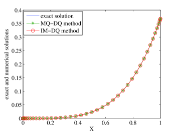
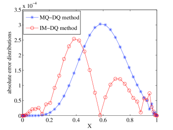
Figure 2: The exact and numerical solutions (left) and absolute error distributions (right) at $t=1$ by using $M=40$ and $\epsilon=0.0312$, $0.0511$ for MQ-DQ and IM-DQ methods, respectively.

Example 5.3. Consider the 2D fractional diffusion equation

$$\frac{\partial u(x,y,t)}{\partial t}-\kappa_{1}(x,y)\mathcal{D}^{\alpha_{1}}_{\theta_{1}}u(x,y,t)-\kappa_{2}(x,y)\mathcal{D}^{\alpha_{2}}_{\theta_{2}}u(x,y,t)=f(x,y,t),$$

on the square domain $[0,1]\times[0,1]$ in two separate cases. The former utilizes the regularly distributed nodal points, while the latter chooses the irregularly distributed nodal points. To compare with FDM Ref14 , we extract the regular nodal distribution from the structured meshes generated by FreeFem++. The computational parameters of these two cases are arranged as follows:

• Letting $\alpha_{1}=1.8$, $\alpha_{2}=1.6$, $\theta_{1}=0$, $\theta_{2}=\pi/2$, $\kappa_{1}(x,y)=\frac{\Gamma(2.2)x^{2.8}y}{6}$, $\kappa_{2}(x,y)=\frac{2xy^{2.6}}{\Gamma(4.6)}$, and the source function $f(x,y,t)=-e^{-t}(1+2xy)x^{3}y^{3.6}$, solve the above equation with the initial and boundary conditions $u_{0}(x,y)=x^{3}y^{3.6}$, $u(0,y,t)=u(x,0,t)=0$, $u(1,y,t)=e^{-t}y^{3.6}$, and $u(x,1,t)=e^{-t}x^{3}$. The exact solution is given by $u(x,y,t)=e^{-t}x^{3}y^{3.6}$.

• Letting $\alpha_{1}=1.8$, $\theta_{1}=\pi/4$, $\kappa_{1}(x,y)=x^{\alpha_{1}}$, $\kappa_{2}(x,y)=0$, and the source function $f(x,y,t)=-e^{-t}x^{2}y^{2}-e^{-t}x^{\alpha_{1}}f^{*}(x,y,t)$ with

  $$f^{*}(x,y,t)=\left\{\begin{array}[]{ll}\frac{2^{1-\frac{\alpha_{1}}{2}}y^{2-\alpha_{1}}\big{(}(\alpha_{1}-4)(\alpha_{1}-3)x^{2}-2(\alpha_{1}-4)\alpha_{1}xy+(\alpha_{1}-1)\alpha_{1}y^{2}\big{)}}{\Gamma(5-\alpha_{1})},\ \ x\geqslant y,\\ \frac{2^{1-\frac{\alpha_{1}}{2}}x^{2-\alpha_{1}}\big{(}(\alpha_{1}-1)\alpha_{1}x^{2}-2(\alpha_{1}-4)\alpha_{1}xy+(\alpha_{1}-4)(\alpha_{1}-3)y^{2}\big{)}}{\Gamma(5-\alpha_{1})},\ \ x<y,\end{array}\right.$$

  solve the above equation with the initial and boundary conditions $u_{0}(x,y)=x^{2}y^{2}$, $u(0,y,t)=u(x,0,t)=0$, $u(1,y,t)=e^{-t}y^{2}$, and $u(x,1,t)=e^{-t}x^{2}$. It can be verified that the exact solution is $u(x,y,t)=e^{-t}x^{2}y^{2}$.

In the second case, the source function suffers relatively complex mathematical structure since $\theta_{1}$ does not along the axis directions. In Table 3, we give a comparison between FDM and DQ methods in term of $e_{\infty}(\tau,M)$ at $t=1$ for the case of (i) with $N=\sqrt{M+1}-1$, $c^{*}=0.98$ for Multiquadrics and $c^{*}=1.22$ for Inverse Multiquadrics. The regular distribution of nodal points with $M=440$ and the corresponding absolute error distribution of MQ-DQ method are shown in Fig. 3. For the case of (ii), we list the numerical results at $t=1$ of DQ methods in Table 4 by using the scattered nodal points of total numbers $74$, $144$, $234$, and $424$, with $N=2000$, $c^{*}=0.89$ for Multiquadrics and $c^{*}=1.25$ for Inverse Multiquadrics. In Fig. 4, we exhibit the used irregular distributions of nodal points, and in Fig. 5, by resetting $M=518$ and $\epsilon=8.6924$, we compare the exact and numerical solutions at $t=1$ created by GA-DQ method. As expected, DQ methods work well on both regular and irregular nodal distributions and yield the approximations that are in perfect agreement with the exact ones. It is also drawn that our methods achieve the errors in the same scale of magnitude as FDM with less nodal numbers.

Table 3: A comparison of FDM and DQ methods at $t=1$ when $N=\sqrt{M+1}-1$.

$M$	FDM Ref14		$M$	MQ-DQ method		IM-DQ method
	$e_{\infty}(\tau,M)$	Cov. rate		$e_{\infty}(\tau,M)$	Cov. rate	$e_{\infty}(\tau,M)$	Cov. rate
120	1.2629e-03	-	99	1.2391e-03	-	3.2338e-03	-
440	6.7325e-04	1.88	195	5.3030e-04	2.5222	1.5975e-03	2.0959
1680	3.4824e-04	1.93	288	3.3018e-04	2.4405	9.9305e-04	2.4487
6560	1.7660e-04	1.97	440	1.9823e-04	2.4144	5.5787e-04	2.7290

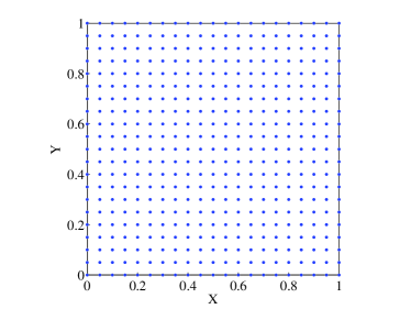
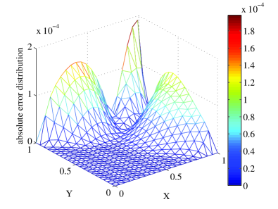
Figure 3: The nodal distribution with $M=440$ and the absolute error distribution of MQ-DQ method.

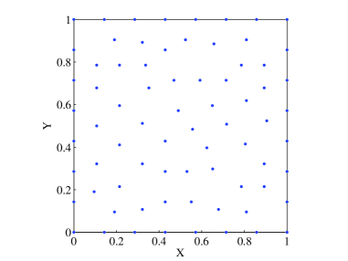
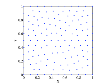
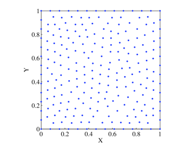
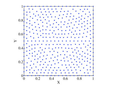
Figure 4: The nodal distributions with nodal numbers $74$, $144$, $234$, and $424$ for Example 5.3.

Table 4: The numerical results at $t=1$ with $N=2000$ and $\alpha=1.8$ for Example 5.3.

$M$	MQ-DQ method		IM-DQ method
	$e_{2}(\tau,M)$	$e_{\infty}(\tau,M)$	$e_{2}(\tau,M)$	$e_{\infty}(\tau,M)$
73	4.5310e-04	1.6351e-03	9.5684e-04	2.8237e-03
143	2.6755e-04	9.3234e-04	4.6647e-04	1.4306e-03
233	8.8580e-05	3.5897e-04	1.6103e-04	6.1178e-04
423	2.6730e-05	1.2532e-04	4.7417e-05	1.7907e-04

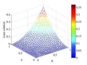
Figure 5: The exact and numerical solutions created by GA-DQ method for Example 5.3.

Example 5.4. Consider the 2D fractional diffusion equation

$$\frac{\partial u(x,y,t)}{\partial t}-x^{\alpha_{1}}\mathcal{D}^{\alpha_{1}}_{\theta_{1}}u(x,y,t)-(1.5-x-0.5y)^{\alpha_{2}-3}\mathcal{D}^{\alpha_{2}}_{\theta_{2}}u(x,y,t)=f(x,y,t),$$

on the trapezoidal domain as shown in Fig. 6, with $\theta_{1}=0$, $\theta_{2}=\pi$, the exact solution $u(x,y,t)=e^{-t}x^{3}(0.5(3-y)-x)^{3}$, the source function

$$f(x,y,t)=-e^{-t}x^{3}(0.5(3-y)-x)^{3}-e^{-t}(g^{*}_{1}(\alpha_{1},x,3-y)+g^{*}_{2}(\alpha_{2},x,y-3)),$$

and the initial and boundary conditions taken from $u(x,y,t)$, where

$$g^{*}_{1}(\alpha,x,y) =\frac{0.75x^{3}y^{3}}{\Gamma(4-\alpha)}-\frac{18x^{4}y^{2}}{\Gamma(5-\alpha)}+\frac{180x^{5}y}{\Gamma(6-\alpha)}-\frac{720x^{6}}{\Gamma(7-\alpha)},$$

$$g^{*}_{2}(\alpha,x,y) =\frac{0.75(\alpha-2)(\alpha-1)\alpha y^{3}+18(\alpha-1)\alpha xy^{2}+180\alpha x^{2}y+720x^{3}}{\Gamma(7-\alpha)}.$$

Let $\alpha_{1}=1.1$, $\alpha_{2}=1.3$, and $N=5000$. We run the algorithm with $c^{*}=0.75$ for Multiquadrics and $c^{*}=1.05$ for Inverse Multiquadrics by using the scattered nodal points of total numbers 66, 171, 287, and 437, which are plotted in Fig. 6, respectively. Table 5 reports the errors of the numerical solutions of DQ methods with respect to the exact solution at $t=1$ at length. It is evident that, under the chosen $\epsilon$’s, the proposed methods are stable and convergent on this trapezoidal domain. Using the last nodal distribution plotted in Fig. 6 and its corresponding $\epsilon$, a comparison between the exact and numerical solutions at $t=1$ created by IM-DQ method is presented in Fig. 7, where no obvious difference can be observed from these two graphs.

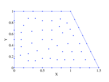
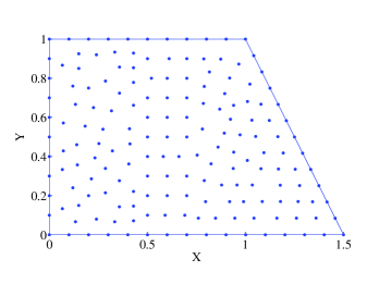
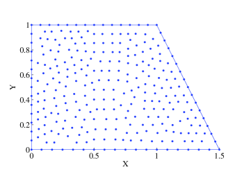
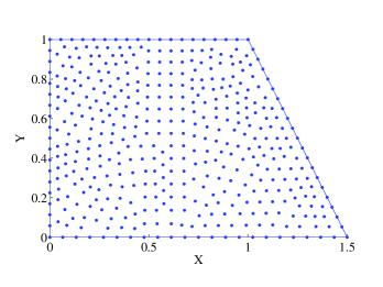
Figure 6: The nodal distributions with nodal numbers $66$, $171$, $287$, and $437$ for Example 5.4.

Table 5: The numerical results at $t=1$ with $N=5000$, $\alpha_{1}=1.1$, and $\alpha_{2}=1.3$ for Example 5.4.

$M$	MQ-DQ method		IM-DQ method
	$e_{2}(\tau,M)$	$e_{\infty}(\tau,M)$	$e_{2}(\tau,M)$	$e_{\infty}(\tau,M)$
65	2.3564e-04	6.9019e-04	3.1638e-04	9.7823e-04
170	1.8822e-04	6.3616e-04	2.2830e-04	7.6927e-04
286	1.0976e-04	4.3639e-04	1.3165e-04	5.2928e-04
436	6.9543e-05	2.7613e-04	8.4616e-05	3.5031e-04

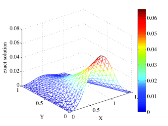
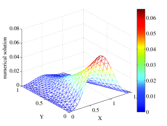
Figure 7: The exact and numerical solutions created by IM-DQ method for Example 5.4.

Example 5.5. In this test, consider the 2D fractional diffusion equation

$$\frac{\partial u(x,y,t)}{\partial t}-\frac{y^{\alpha}}{2}\mathcal{D}^{\alpha}_{\theta}u(x,y,t)=f(x,y,t),$$

on $\Omega=\{(x,y):(x-0.5)^{2}+(y-0.5)^{2}\leqslant 0.25\}$, with $\theta=0$, $\alpha=1.9$, the exact solution $u(x,y,t)=t^{2}(x-0.5+\sqrt{0.25-(y-0.5)^{2}})^{2}y^{2}$, the source function

$$f(x,y,t) =2t(x-0.5+\sqrt{0.25-(y-0.5)^{2}})^{2}y^{2}$$

$$\quad-\frac{t^{2}(x-0.5+\sqrt{0.25-(y-0.5)^{2}})^{2-\alpha}y^{2+\alpha}}{\Gamma(3-\alpha)},$$

and the initial and boundary conditions taken from the exact solution. The computational domain as well as the involved nodal distributions with nodal numbers 54, 80, 201, and 402 are displayed in Fig. 8, respectively. To see the actual performance of our methods, we compute the numerical results at $t=1$ with $N=5000$ and document them side by side in Table 6 by using $c^{*}=0.85$ for Inverse Multiquadrics and the data sets consisting of 5.4216, 5.9814, 7.5306, and 8.9554 for the shape parameter contained in Gaussians. It is found that our methods show their capability to deal with the fractional problem on circular domains even if the nodal distributions are irregular. Besides, under the given $\epsilon$’s, IM-DQ method outperforms GA-DQ method in term of overall accuracy. Resetting $M=472$ together with $\epsilon=10.3221$, we compare the exact and numerical solutions at $t=1$ created by GA-DQ method in Fig. 9. It is observed that our method produces the approximation with sufficiently small errors, which can not be visually distinguished from the exact one. This confirms the effectiveness of the proposed methods once more.

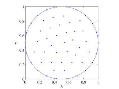
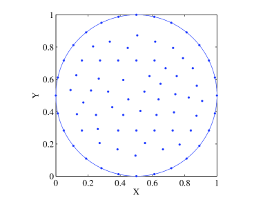
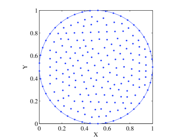
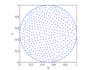
Figure 8: The nodal distributions with nodal numbers $54$, $80$, $201$, and $402$ for Example 5.5.

Table 6: The numerical results at $t=1$ with $N=5000$ and $\alpha=1.9$ for Example 5.5.

$M$	IM-DQ method		GA-DQ method
	$e_{2}(\tau,M)$	$e_{\infty}(\tau,M)$	$e_{2}(\tau,M)$	$e_{\infty}(\tau,M)$
53	4.4502e-03	2.1437e-02	1.2039e-02	5.8457e-02
79	2.9459e-03	1.3023e-02	8.8637e-03	3.8900e-02
200	7.3905e-04	4.0762e-03	1.8664e-03	1.0135e-02
401	3.8098e-04	2.3782e-03	8.9460e-04	6.1255e-03

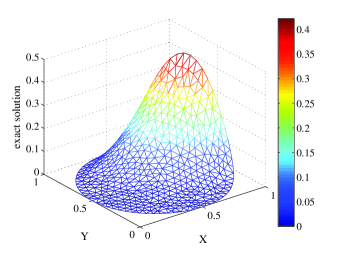
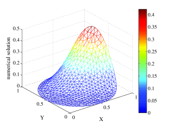
Figure 9: The exact and numerical solutions created by GA-DQ method for Example 5.5.

Example 5.6. In the last test, consider the 2D fractional diffusion equation

$$\frac{\partial u(x,y,t)}{\partial t}-x^{\alpha}y^{\alpha}\sum^{3}_{l=1}\mathcal{D}^{\alpha}_{\theta_{l}}u(x,y,t)=f(x,y,t),$$

on the L-shaped domain as shown in Fig. 10, with $\theta_{1}=0$, $\theta_{2}=\pi/4$, and $\theta_{3}=\pi/2$, subjected to the initial and boundary conditions taken from the exact solution $u(x,y,t)=t^{3}x^{2}y^{2}$. The source function is manufactured by

$$f(x,y,t) =3t^{2}x^{2}y^{2}-t^{3}x^{\alpha}y^{\alpha}\bigg{(}f^{*}(x,y,t)+2\frac{x^{2-\alpha}y^{2}+x^{2}y^{2-\alpha}}{\Gamma(3-\alpha)}\bigg{)},$$

with $\alpha_{1}=\alpha$ in $f^{*}(x,y,t)$ declared above. Letting $\epsilon$ be 0.2128 in Multiquadrics, 0.3445 in Inverse Multiquadrics, and 4.6880 in Gaussians, we examine the convergence of DQ methods at $t=0.5$ versus the variation of $\alpha$ with $N=1000$ on the scattered nodal points of total number $593$. The numerical results are reported in Table 7. The used irregular nodal distribution and the absolute error distribution of IM-DQ method for $\alpha=1.5$ are plotted in Fig. 10, respectively. As one can see, the errors decay as $\alpha$ increases in addition to a special case of $\alpha=2.0$ for $e_{\infty}(\tau,M)$, and MQ-DQ method outperforms IM-DQ, GA-DQ methods in term of overall accuracy under the given $\epsilon$’s.

Table 7: The numerical results at $t=0.5$ with $N=2000$ and $M=592$ for Example 5.6

$\alpha$	MQ-DQ method		IM-DQ method		GA-DQ method
	$e_{2}(\tau,M)$	$e_{\infty}(\tau,M)$	$e_{2}(\tau,M)$	$e_{\infty}(\tau,M)$	$e_{2}(\tau,M)$	$e_{\infty}(t,M)$
1.2	1.5847e-04	5.3015e-04	1.4751e-04	8.9850e-04	2.9393e-04	1.5306e-03
1.5	1.0553e-04	4.0805e-04	1.1669e-04	6.3374e-04	2.5013e-04	1.1697e-03
1.8	6.3716e-05	3.6591e-04	8.9356e-05	4.8952e-04	1.9519e-04	8.8947e-04
2.0	5.2515e-05	3.8395e-04	7.2907e-05	4.4158e-04	1.5855e-04	7.1631e-04

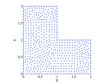
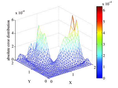
Figure 10: The nodal distribution with $M=592$ and the absolute error distribution of IM-DQ method.

6 Conclusion

The multi-dimensional space-fractional diffusion equations are essential part of fractional PDEs and have been one of principle concerns in mathematical physics, but solving these types of equations appears to be somewhat challenging due to the global correlation of fractional derivatives, especially on irregular domains. In this research, by using Multiquadric, Inverse Multiquadric and Gaussian RBFs as trial functions, the DQ formulations for fractional directional derivatives of Caputo type are presented. Then, three effective DQ methods are proposed for the space-fractional diffusion equations on 2D irregular domains via discretizing the resultant ODEs by employing the Crank-Nicolson scheme. These methods enjoy some appealing advantages such as low occupancy cost, truly mesh-free, and the adaptability to arbitrary domains, which make they compare favorably to some of traditional methods as FDM. The computational accuracy relies on the nodal number, shape parameter, the complexity of fractional models, and the other potential factors. The codes are utilized to treat the fractional problems on square, trapezoidal, circular, and L-shaped domains, respectively, and the outcomes have demonstrated that our methods are capable of capturing the exact solutions under the condition that the shape parameters are well prepared. Due to the characteristics of RBFs, these DQ methods are insensitive to dimensional change, which means that they can be generalized to three-dimensions without a significant increase in computational burden. This merit evidently offers us a possibility to simulate the other space-fractional problems in high-dimensions with complex boundaries arising in the fields of anomalous dispersion, fluid dynamics, conservative systems, genetic propagation, and viscoelastic materials.

- (1) Adams, E.E., Gelhar, L.W.: Field study of dispersion in a heterogeneous aquifer: 2. Spatial moments analysis. Water Resour. Res. 28(12), 3293–3307 (1992)
- (2) Agrawal, O.P.: Solution for a fractional diffusion-wave equation defined in a bounded domain. Nonlinear Dyn. 29(1), 145–155 (2002)
- (3) Atluri, S.N., Zhu, T.L.: The meshless local Petrov-Galerkin (MLPG) approach for solving problems in elasto-statics. Comput. Mech. 25(2-3), 169–179 (2000)
- (4) Bellman, R., Casti, J.: Differential quadrature and long-term integration. J. Math. Anal. Appl. 34(2), 235–238 (1971)
- (5) Bellman, R., Kashef, B., Lee, E.S., Vasudevan, R.: Differential quadrature and splines. Comput. Math. Appl. 1(3), 371–376 (1975)
- (6) Bhrawy, A.H., Baleanu, D.: A spectral Legendre–Gauss–Lobatto collocation method for a space-fractional advection diffusion equations with variable coefficients. Rep. Math. Phys. 72(2), 219–233 (2013)
- (7) Bonzani, I.: Solution of nonlinear evolution problems by parallelized collocation-interpolation methods. Comput. Math. Appl. 34(12), 71–79 (1997)
- (8) Bueno-Orovio, A., Kay, D., Burrage, K.: Fourier spectral methods for fractional-in-space reaction-diffusion equations. BIT 54(4), 937–954 (2014)
- (9) Carlson, R.E., Foley, T.A.: The parameter R2 in multiquadric interpolation. Comput. Math. Appl. 21(9), 29–42 (1991)
- (10) Carpinteri, A., Mainardi, F.: Fractals and Fractional Calculus in Continuum Mechanics. Springer-Verlag, Wien (1997)
- (11) del Castillo-Negrete, D., Carreras, B.A., Lynch, V.E.: Fractional diffusion in plasma turbulence. Phys. Plasmas 11(8), 3854–3864 (2004)
- (12) Chen, Y.M., Wu, Y.B., Cui, Y.H., Wang, Z.Z., Jin, D.M.: Wavelet method for a class of fractional convection-diffusion equation with variable coefficients. J. Comput. Sci. 1(3), 146–149 (2010)
- (13) Chen, Y.P., Lee, J., Eskandarian, A.: Meshless Methods in Solid Mechanics. Springer, Berlin (2006)
- (14) Cheng, A.H.D., Golberg, M.A., Kansa, E.J., Zammito, G.: Exponential convergence and H-c multiquadric collocation method for partial differential equations. Numer. Meth. Part. D. E. 19(5), 571–594 (2003)
- (15) Cheng, R.J., Sun, F.X., Wang, J.F.: Meshless analysis of two-dimensional two-sided space-fractional wave equation based on improved moving least-squares approximation. Int. J. Comput. Math (2017). DOI: 10.1080/00207160.2017.1291933
- (16) Deng, W.H.: Finite element method for the space and time fractional Fokker–Planck equation. SIAM J. Numer. Anal. 47(1), 204–226 (2008)
- (17) Deng, W.H., Li, B.Y., Tian, W.Y., Zhang, P.W.: Boundary problems for the fractional and tempered fractional operators. SIAM Journal on Multiscale Modeling and Simulation (In Press)
- (18) Ding, H.F.: General Padé approximation method for time-space fractional diffusion equation. J. Comput. Appl. Math. 299, 221–228 (2016)
- (19) Doha, E.H., Bhrawy, A.H., Baleanu, D., Ezz-Eldien, S.S.: The operational matrix formulation of the Jacobi tau approximation for space fractional diffusion equation. Adv. Differ. Equ. 2014, 231 (2014)
- (20) Du, N., Wang, H.: A fast finite element method for space-fractional dispersion equations on bounded domains in . SIAM J. Sci. Comput. 37(3), A1614–A1635 (2015)
- (21) Elhay, S., Kautsky, J.: Algorithm 655: IQPACK: FORTRAN subroutines for the weights of interpolatory quadratures. Acm. T. Math. Softwar. 13(4), 399–415 (1987)
- (22) Ervin, V.J., Roop, J.P.: Variational formulation for the stationary fractional advection dispersion equation. Numer. Meth. Part. D. E. 22(3), 558–576 (2006)
- (23) Fasshauer, G.E., Zhang, J.G.: On choosing “optimal” shape parameters for RBF approximation. Numer. Algor. 45(1), 345–368 (2007)
- (24) Feng, L.B., Zhuang, P., Liu, F., Turner, I., Anh, V., Li, J.: A fast second-order accurate method for a two-sided space-fractional diffusion equation with variable coefficients. Comput. Math. Appl. 73(6), 1155–1171 (2017)
- (25) Gingold, R.A., Monaghan, J.J.: Smooth particle hydrodynamics: theory and applications to non spherical stars. Monthly Notices of the Royal Astronomical Society 181(3), 375–389 (1977)
- (26) Hejazi, H., Moroney, T., Liu, F.: Stability and convergence of a finite volume method for the space fractional advection-dispersion equation. J. Comput. Appl. Math. 255, 684–697 (2014)
- (27) Ichise, M., Nagayanagi, Y., Kojima, T.: An analog simulation of non-integer order transfer functions for analysis of electrode processes. J. Electroanal. Chem. 33(2), 253–265 (1971)
- (28) Jia, J.H., Wang, H.: A fast finite volume method for conservative space-fractional diffusion equations in convex domains. J. Comput. Phys. 310, 63–84 (2016)
- (29) Ju, L.L., Gunzburger, M., Zhao, W.D.: Adaptive finite element methods for elliptic PDEs based on conforming centroidal Voronoi-Delaunay triangulations. SIAM J. Sci. Comput. 28(6), 2023–2053 (2006)
- (30) Liu, F., Zhuang, P., Turner, I., Anh, V., Burrage, K.: A semi-alternating direction method for a 2-D fractional FitzHugh–Nagumo monodomain model on an approximate irregular domain. J. Comput. Phys. 293, 252–263 (2015)
- (31) Liu, G.R., Gu, Y.T.: An Introduction to Meshfree Methods and their Programming. Springer, Berlin (2005)
- (32) Liu, G.R., Gu, Y.T., Dai, K.Y.: Assessment and applications of point interpolation methods for computational mechanics. Int. J. Numer. Meth. Engng. 59(10), 1373–1397 (2004)
- (33) Liu, Q., Liu, F., Gu, Y.T., Zhuang, P., Chen, J., Turner, I.: A meshless method based on Point Interpolation Method (PIM) for the space fractional diffusion equation. Appl. Math. Comput. 256, 930–938 (2015)
- (34) Liu, W.K., Jun, S., Zhang, Y.F.: Reproducing kernel particle methods. Int. J. Numer. Methods Fluids. 20, 1081–1106 (1995)
- (35) Luh, L.T.: The shape parameter in the Gaussian function II. Eng. Anal. Bound. Elem. 37(6), 988–993 (2013)
- (36) Mainardi, F.: The fundamental solutions for the fractional diffusion-wave equation. Appl. Math. Lett. 9(6), 23–28 (1996)
- (37) Meerschaert, M.M., Scheffler, H.P., Tadjeran, C.: Finite difference methods for two-dimensional fractional dispersion equation. J. Comput. Phys. 211(1), 249–261 (2006)
- (38) Meerschaert, M.M., Tadjeran, C.: Finite difference approximations for two-sided space-fractional partial differential equations. Appl. Numer. Math. 56(1), 80–90 (2006)
- (39) Melenk, J.M., Babuška, I.: The partition of unity finite element method: Basic theory and applications. Comput. Methods Appl. Mech. Engrg. 139(1-4), 289–314 (1996)
- (40) Nayroles, B., Touzot, G., Villon, P.: Generalizing the finite element method: diffuse approximation and diffuse elements. Comput. Mech. 10(5), 307–318 (1992)
- (41) Nezza, E.D., Palatucci, G., Valdinoci, E.: Hitchhiker’s guide to the fractional Sobolev spaces. Bull. Sci. math. 136(5), 521–573 (2012)
- (42) Nigmatullin, R.R.: The realization of the generalized transfer equation in a medium with fractal geometry. Phys. Status. Solidi. B 133(1), 425–430 (1986)
- (43) Onate, E., Idelsohn, S., Zienkiewicz, O.C., Taylor, R.L.: A finite method in computational mechanics: applications to convective transport and fluid flow. Int. J. Numer. Meth. Engng. 39(22), 3839–3866 (1996)
- (44) Pang, G.F., Chen, W., Fu, Z.J.: Space-fractional advection-dispersion equations by the Kansa method. J. Comput. Phys. 293, 280–296 (2015)
- (45) Pang, G.F., Chen, W., Sze, K.Y.: Gauss-Jacobi-type quadrature rules for fractional directional integrals. Comput. Math. Appl. 66(5), 597–607 (2013)
- (46) Podlubny, I.: Fractional Differential Equations. Academic Press, San Diego, CA (1999)
- (47) Qiu, L.L., Deng, W.H., Hesthaven, J.S.: Nodal discontinuous Galerkin methods for fractional diffusion equations on 2D domain with triangular meshes. J. Comput. Phys. 298, 678–694 (2015)
- (48) Quan, J.R., Chang, C.T.: New insights in solving distributed system equations by the quadrature method–I. Analysis. Comput. Chem. Eng. 13(7), 779–788 (1989)
- (49) Ray, S.S.: Analytical solution for the space fractional diffusion equation by two-step Adomian Decomposition Method. Commun. Nonlinear Sci. Numer. Simulat. 14(4), 1295–1306 (2009)
- (50) Ren, R.F., Li, H.B., Jiang, W., Song, M.Y.: An efficient Chebyshev-tau method for solving the space fractional diffusion equations. Appl. Math. Comput. 224, 259–267 (2013)
- (51) Rippa, S.: An algorithm for selecting a good value for the parameter in radial basis function interpolation. Adv. Comput. Math. 11(2), 193–210 (1999)
- (52) Saadatmandi, A., Dehghan, M.: A tau approach for solution of the space fractional diffusion equation. Comput. Math. Appl. 62(3), 1135–1142 (2011)
- (53) Sarra, S.A., Sturgill, D.: A random variable shape parameter strategy for radial basis function approximation methods. Eng. Anal. Bound. Elem. 33(11), 1239–1245 (2009)
- (54) Shu, C., Richards, B.E.: Application of generalized differential quadrature to solve two-dimensional incompressible Navier-Stokes equations. Int. J. Numer. Methods Fluids 15(7), 791–798 (1992)
- (55) Sousa, E.: Numerical approximations for fractional diffusion equations via splines. Comput. Math. Appl. 62(3), 938–944 (2011)
- (56) Sun, F.X., Wang, J.F.: Interpolating element-free Galerkin method for the regularized long wave equation and its error analysis. Appl. Math. Comput. 315, 54–69 (2017)
- (57) Sun, F.X., Wang, J.F., Cheng, Y.M.: An improved interpolating element-free Galerkin method for elastoplasticity via nonsingular weight functions. Int. J. Appl. Mechanics 08(08), 1650,096 (2016)
- (58) Tian, W.Y., Zhou, H., Deng, W.H.: A class of second order difference approximations for solving space fractional diffusion equations. Math. Comp. 84(294), 1703–1727 (2015)
- (59) Vong, S., Lyu, P., Chen, X., Lei, S.L.: High order finite difference method for time-space fractional differential equations with Caputo and Riemann-Liouville derivatives. Numer. Algor. 72(1), 195–210 (2016)
- (60) Wang, H., Basu, T.S.: A fast finite difference method for two-dimensional space-fractional diffusion equations. SIAM J. Sci. Comput. 34(5), A2444–A2458 (2012)
- (61) Wu, Y.L., Shu, C.: Development of RBF-DQ method for derivative approximation and its application to simulate natural convection in concentric annuli. Comput. Mech. 29(6), 477–485 (2002)
- (62) Xu, Q.W., Hesthaven, J.S.: Discontinuous Galerkin method for fractional convection-diffusion equations. SIAM J. Numer. Anal. 52(1), 405–423 (2014)
- (63) Yang, Z., Yuan, Z., Nie, Y., Wang, J., Zhu, X., Liu, F.: Finite element method for nonlinear Riesz space fractional diffusion equations on irregular domains. J. Comput. Phys. 330, 863–883 (2017)
- (64) Yıldırım, A., Koçak, H.: Homotopy perturbation method for solving the space-time fractional advection-dispersion equation. Adv. Water Resour. 32(12), 1711–1716 (2009)
- (65) Yuan, Z.B., Nie, Y.F., Liu, F., Turner, I., Zhang, G.Y., Gu, Y.T.: An advanced numerical modeling for Riesz space fractional advection–dispersion equations by a meshfree approach. Appl. Math. Model. 40(17), 7816–7829 (2016)
- (66) Zayernouri, M., Karniadakis, G.E.: Fractional spectral collocation methods for linear and nonlinear variable order FPDEs. J. Comput. Phys. 293, 312–338 (2015)
- (67) Zeng, F.H., Liu, F.W., Li, C.P., Burrage, K., Turner, I., Anh, V.: A Crank–Nicolson ADI spectral method for a two-dimensional Riesz space fractional nonlinear reaction-diffusion equation. SIAM J. Numer. Anal. 52(6), 2599–2622 (2014)
- (68) Zhu, X.G., Nie, Y.F., Wang, J.G., Yuan, Z.B.: A numerical approach for the Riesz space-fractional Fisher’ equation in two-dimensions. Int. J. Comput. Math. 94(2), 296–315 (2017)