Adaptive Time-stepping Schemes for the Solution of the Poisson-Nernst-Planck Equations

Abstract

The Poisson-Nernst-Planck equations with generalized Frumkin-Butler-Volmer boundary conditions (PNP-FBV) describe ion transport with Faradaic reactions, and have applications in a number of fields. In this article, we develop an adaptive time-stepping scheme for the solution of the PNP-FBV system based on two time-stepping methods: a fully-implicit (VSBDF2) method, and a semi-implicit (VSSBDF2) method. We present simulations under both current and voltage boundary conditions and demonstrate the ability to simulate a large range of parameters, including any value of the singular perturbation parameter $\epsilon$. When the underlying dynamics is one that would have the solutions converge to a steady-state solution, we observe that the adaptive time-stepper based on the VSSBDF2 method produces solutions that “nearly” converge to the steady-state solution and that, simultaneously, the time-step sizes stabilize to a limiting size $dt_{\infty}$. In the companion to this article [1], we linearize the SBDF2 scheme about the steady-state solution, and demonstrate that the linearized scheme is conditionally stable, and that this conditional stability is the cause of the adaptive time-stepper’s behaviour. While the adaptive time-stepper based on the fully-implicit (VSBDF2) method is not subject to such time-step stability restrictions, the required nonlinear solve incurs additional computational cost. We profile both methods to identify regimes of the perturbation parameter $\epsilon$ where one method is favourable over the other. The matlab code used in this work can be found at https://github.com/daveboat/vssimex_pnp .

1 Introduction

The Poisson-Nernst-Planck (PNP) equations describe the transport of charged species subject to diffusion and electromigration. They have wide applicability in electrochemistry, and have been used to model a number of different systems, including porous media [2, 3, 4, 5], microelectrodes [6, 7], ion-exchange membranes [8, 9], electrokinetic phenomena [10, 11, 12], ionic liquids [13, 14], electrochemical thin films [15, 16, 17], fuel cells [18], supercapacitors [19], and more.

The one-dimensional, nondimensionalized PNP equations for a media with $2$ mobile species is

$$\frac{\partial c_{\pm}}{\partial t} =-\frac{\partial}{\partial x}\left[-\frac{\partial c_{\pm}}{\partial x}-z_{\pm}\,c_{\pm}\,\frac{\partial\phi}{\partial x}\right],\qquad t>0,\,x\in(0,1),$$ (1)

$$-\epsilon^{2}\frac{\partial^{2}\phi}{\partial x^{2}} =\frac{1}{2}\left(z_{+}\,c_{+}+z_{-}\,c_{-}\right),\qquad\qquad\qquad x\in(0,1),$$ (2)

where $c_{\pm}$ and $z_{\pm}$ are the concentration and charge number of the positive/negative ion, $\phi$ is the potential and $\epsilon$ is the ratio of the Debye screening length to the inter-electrode width $L$. This width is used in the nondimensionalization of the original modelling equations [20]; the domain $(0,L)$ is rescaled to $(0,1)$. We consider a model in which the anion and cation have a single charge ($z_{\pm}=\pm 1$) and the anion has no charge-transfer reactions at the electrode: $c_{-}$ has no-flux boundary conditions:

$$-\left(-\frac{\partial c_{-}}{\partial x}+\,c_{-}\,\frac{\partial\phi}{\partial x}\right)\bigg{|}_{x=0}\mkern-12.0mu=\left(-\frac{\partial c_{-}}{\partial x}+\,c_{-}\,\frac{\partial\phi}{\partial x}\right)\bigg{|}_{x=1}=0.$$ (3)

The cation is assumed to have a reaction at the electrodes involving the transfer of one electron; this is modelled using generalized Frumkin-Butler-Volmer (FBV) boundary conditions:

$$-\left(-\frac{\partial c_{+}}{\partial x}-\,c_{+}\,\frac{\partial\phi}{\partial x}\right)\bigg{|}_{x=0}\mkern-12.0mu =F(t):=4k_{c,a}\,c_{+}(0,t)\,e^{-0.5\;\Delta\phi_{\text{left}}}-4\,j_{r,a}\,e^{0.5\;\Delta\phi_{\text{left}}},$$ (4)

$$\left(-\frac{\partial c_{+}}{\partial x}-\,c_{+}\,\frac{\partial\phi}{\partial x}\right)\bigg{|}_{x=1}\mkern-12.0mu =G(t):=4k_{c,c}\,c_{+}(1,t)\,e^{-0.5\;\Delta\phi_{\text{right}}}-4\,j_{r,c}\,e^{0.5\;\Delta\phi_{\text{right}}},$$ (5)

where $k_{c,a}$, $k_{c,c}$, $j_{r,a}$, and $j_{r,c}$ are reaction rate parameters; the second letter in the subscripts ($a$ and $c$) refer to the anode and cathode, respectively. Equations (4)–(5) model the electrodeposition reaction

$$\ce{C^{+}+e^{-}<=>M}$$ (6)

where M represents the electrode material.

The Stern layer is a compact layer of charge that occurs in the electrolyte next to an electrode surface [21, 22]; $\lambda_{S}$ denotes the effective width of this layer. In equations (4)–(5), $\Delta\phi_{\text{left}}$ and $\Delta\phi_{\text{right}}$ refer to the potential differences across the Stern layers that occur at the anode and cathode respectively. Specifically,

$$\Delta\phi_{\text{left}}=\phi_{\text{anode}}-\phi(0,t)=-\phi(0,t),\;\Delta\phi_{\text{right}}=\phi_{\text{cathode}}-\phi(1,t)=v(t)-\phi(1,t)$$ (7)

where the potential at the anode has been set to zero and $v(t)$ denotes the potential at the cathode.

The Poisson equation (2) uses a mixed (or Robin) boundary condition [15, 16, 17],

$$-\epsilon\,\delta\;\frac{\partial\phi}{\partial x}\bigg{|}_{x=0} =\Delta\phi_{\text{left}}:=-\phi(0,t),$$ (8)

$$+\epsilon\,\delta\;\frac{\partial\phi}{\partial x}\bigg{|}_{x=1} =\Delta\phi_{\text{right}}:=v(t)-\phi(1,t),$$ (9)

where $\delta=\lambda_{S}/L$. Finally, there is an ODE which ensures conservation of electrical current at the electrode [23, 24],

$$-\frac{\epsilon^{2}}{2}\,\frac{d\;}{dt}\phi_{x}(1,t)=j_{\text{ext}}(t)-\left[k_{c,c}\,c_{+}\left(1,t\right)\,e^{-0.5\;\Delta\phi_{\text{right}}}-j_{r,c}\,e^{0.5\;\Delta\phi_{\text{right}}}\right],$$ (10)

where $j_{\text{ext}}(t)$ is the current through the device. We refer to the PNP equations with the generalized Frumkin-Butler-Volmer boundary conditions as the PNP-FBV system.

Considering more than two charged species or reactions involving the transfer of more than one electron is a straight-forward generalization [25, 26]. If the model is extended to include adsorption effects at the electrodes, there would be an additional ODE describing the dynamics of the fraction of surface coverage for each electrode [27]. If, in addition, the model included temperature and heat transport, there would be another PDE for the temperature [27]. In this work however, we limit ourselves to just the PNP-FBV system.

The device is operated in two regimes — either the current or the voltage at the cathode is externally controlled. If the voltage at the cathode, $v(t)$, is externally controlled then the the PNP-FBV system (1)–(2) with boundary conditions (3)–(5) and (7)–(9) are numerically solved, determining $c_{\pm}$ and $\phi$. The current is found a postiori using equation (10). If the current, $j_{\text{ext}}(t)$, is externally controlled, then equation (10) is part of the PNP-FBV system and the ODE is numerically solved along with the PDEs, determining $c_{\pm}$, $\phi$, and $\phi_{x}(1,t)$ simultaneously. The voltage $v(t)$ is then found a postiori.

Some prior numerical approaches to the PNP and PNP-FBV systems

Though many workers in the field have approximated solutions to the PNP-FBV system using asymptotic methods [28, 29], a numerical method is needed to obtain a full solution. A key mathematical aspect of the PNP-FBV system is that the parameter $\epsilon$ acts as a singular perturbation to the system and results in the formation of boundary layers [30]. This makes numerical simulation of the PNP-FBV system especially challenging.

An accurate, efficient solver for the PNP-FBV equations must take into account the solution’s spatial and temporal characteristics. First, the bulk ($10\epsilon\lesssim x\lesssim 1-10\epsilon$) is approximately electroneutral [31] and so the concentrations and potential are linear or nearly linear there, whereas they are nonlinear, and can change significantly over short distances, near the electrodes ($0<x\lesssim 10\epsilon$ and $1-10\epsilon\lesssim x<1$). A non-uniform mesh which distributes more mesh points near $x=0,1$ is therefore an economical way to discretize the spatial domain. Secondly, many electrochemical systems of interest are subject to sudden changes in forcing, separated by periods with constant or no forcing. This, combined with the transient dynamics driven by initial conditions, gives the problem more than one time-scale, motivating the need for specialized time-stepping methods.

One of the first contributions to the field of time-stepping methods for the Poisson-Nernst-Planck equations, was by Cohen and Cooley [32], who used an explicit time-stepping method with predictor-corrector time-step refinement to solve the electroneutral equations with constant current. The next contribution was by Sandifer and Buck [33], who solved a system of time-independent Nernst-Planck equations with constant current and used an implicit, iterative method to step the displacement field equations. Brumleve and Buck [34] solved the full PNP equations with Chang-Jaffe boundary conditions using Backward Euler time-stepping. In Brumleve and Buck’s method, time-steps were allowed to be variable, but were not adjusted during each step; the method given in the original publication still sees use in more modern work [35]. Murphy et. al. [36] solved the full PNP-FBV system with adaptive steps by treating the discretized parabolic-elliptic system as a differential-algebraic system of ODE’s and algebraic equations, and used a variable-order Gear’s method [37]. It is also worth mentioning here the work of Scharfetter and Gummel [38], who gave a numerical method to solve the drift-diffusion equations (an analogue of the PNP equations in semiconductor physics) using Crank-Nicolson time-stepping.

One recent work where the time-dependent PNP equations (with FBV) are solved is Soestbergen, Biesheuvel and Bazant [24]. They used the commercial finite element software COMSOL, which uses BDF and the generalized-$\alpha$ method [39]. Another is Britz and Strutwolf [40], who simulate a liquid junction using BDF with constant time-steps. Britz [41] also outlines various explicit and implicit multistep methods in his book on computational solutions to the PNP equations.

Our numerical approaches and results of simulations

Our present work differs from previous work (notably Murphy et. al.) by using a splitting method for the parabolic-elliptic system (1)–(2) and differs from other modern computational methods [42] by controlling time-steps adaptively. In this article, we develop and test two adaptive time-steppers for the PNP-FBV system with error control, one of which is semi-implicit (also called implicit-explicit) and one of which is fully-implicit. The adaptivity allows the time-stepper to automatically detect changes in time scales and vary the step size accordingly.

The semi-implicit adaptive time-stepper is based on a second-order variable step-size, semi-implicit, backward differentiation formula (Variable Step-size Semi-implicit Backwards Differentiation Formula, or VSSBDF2 [43]). Its constant step-size counterpart (SBDF2) is used as a time-stepping scheme in a variety of fields in science, engineering and computational mathematics. Axelsson et. al. [44], for example, used SBDF2 with constant steps to solve the time-dependent Navier-Stokes equations. Lecoanet et. al. [45] used a similar method to model combustion equations in stars, and Linde, Persson and Sydow [46] used it to solve the Black-Scholes equation in computational finance. An example of an adaptive SBDF2 time-stepping scheme can be found in Rosam, Jimack and Mullis [47], who use it to study a problem in binary alloy solidification.

The fully-implicit adaptive time-stepper is based on a second-order Variable Step-size, fully-implicit, Backward Differentiation Formula (VSBDF2). Its constant step-size counterpart (BDF2) has the advantage of being unconditionally stable when applied to linear systems that have asymptotically stable steady states. An example of VSBDF2 is Eckert et. al. [48], who use it to model electroplasticity; their scheme is fully-implicit and they do not report any kind of instability or time step stability restriction. However, for nonlinear problems, this numerical stability comes at the cost of needing to perform a computationally expensive nonlinear solve at each time-step.

We apply the (fully-implicit) VSBDF2 and (semi-implicit) VSSBDF2 adaptive time-steppers to the PNP-FBV system with time-dependent imposed forcing (voltage or current). Both time-steppers behave as desired: the time-steps refine by orders of magnitude in response to fast changes in the forcing and coarsen if the forcing is changing slowly (or not at all). See Figure 4.

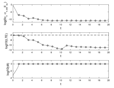
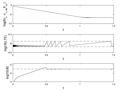
Figure 1: PNP-FBV system (1)–(9) with constant imposed voltage $v(t)=2$, $\epsilon=.05$, and all other physical parameters set to $1$. The initial data is $c_{\pm}(x,0)=1+.1\,\sin(2\pi x)$ and $\phi_{x}(1,0)=0$. A uniform mesh is used: $N=90$ and $L_{1}=L_{2}=L_{3}=1/3$. In the three plots on the left, the (fully-implicit) VSBDF2 adaptive time-stepper is used and, in the three plots on the right, the (semi-implicit) VSSBDF2 adaptive time-stepper is used. In the left plots, open circles are to denote the time steps, after the time-step size $dt$ reaches $dt_{\text{max}}$. The behaviour shown in the right plots between $t=1.25$ and $t=1.5$ is similar to that observed up to $t=20$. Top plots: The logarithm of the maximum deviation of the computed solution $c_{+}$ from the steady state $c_{+,ss}$ at each moment in time: $\log(\|\mathbf{c}_{+}^{n}-\mathbf{c}_{+,ss}\|_{\infty})$. Deviations of $\mathbf{c}_{-}^{n}$ and $\boldsymbol{\phi}^{n}$ from the corresponding steady state profiles behave similarly, as do their time derivatives as approximated using (11). Middle plots: The logarithm of the approximate local truncation error, (17). The dashed lines in both plots indicate $\log(tol\pm range)$. Bottom plots: The logarithm of the time-step size, $dt$, plotted versus time. The dashed line in the left plot indicates the maximum step-size $dt_{\text{max}}$. The dashed line in the right plot indicates the stability restriction $dt^{*}=.0031$ computed using the linear stability analysis presented in Section 5 of the companion paper [1].

However, there are fundamental differences between the (fully-implicit) VSBDF2 and (semi-implicit) VSSBDF2 adaptive time-steppers in the constant-forcing regime. In this regime, the steady-state solution is asymptotically stable. We find that the (fully-implicit) VSBDF2 adaptive time-stepper takes larger and larger time steps until reaching a user-specified maximum time-step $dt_{\text{max}}$ and that solutions converge to the steady-state solution. See Figure 1.

In contrast, we find that the (semi-implicit) VSSBDF2 adaptive time-stepper coarsens its time steps but they stabilize at a limiting time-step size, $dt_{\infty}$, which is smaller than $dt_{\text{max}}$. In addition, we observe that the solution gets close to, but fails to converge to, the stable steady state. In the companion article [1] we perform a linear stability analysis of the SBDF2 scheme about the steady-state solution, and demonstrate that the scheme is conditionally stable with a step size stability restriction $dt^{*}$. We demonstrate that it is this underlying stability restriction that causes the VSSBDF2 adaptive time-stepper to have a limiting time-step size, and present numerical evidence that $dt_{\infty}=dt^{*}$. We find that the stability restriction does not depend significantly on the mesh width. Specifically, $dt_{\infty}$ does not go to zero as the mesh width goes to zero.

We find that $dt_{\infty}\approx\epsilon^{2}$ for small values of the singular perturbation parameter $\epsilon$; as a result the (semi-implicit) VSSBDF2 adaptive time-stepper will take small step sizes for small values of $\epsilon$. Although the time steps can be taken larger when using the fully-implicit VSBDF2 adaptive time-stepper, each time step takes longer due to the nonlinear solve required. We compare performance times for both adaptive time-steppers, and identify regimes of the perturbation parameter $\epsilon$ where the runtime for each method is favourable.

Previous work on time-dependent solutions to the PNP-FBV system [24, 49] took comparably large values, $\epsilon\geq 10^{-3}$, whereas in principle we are able to simulate with any value of $\epsilon$, allowing exploration of a wider range of operating regimes. For example, the adaptivity of the time-stepper allowed us to numerically explore certain standard experimental protocols, such as linear sweep voltammetry, in which a time-dependent voltage or current is imposed [20].

Separately, we explore how the temporal discretization of the boundary conditions affects the accuracy of the (semi-implicit) VSSBDF2 scheme. We find that the “natural” semi-implicit approach to the discretizing boundary conditions — discretizing the boundary conditions by treating the linear term implicitly and extrapolating the nonlinear terms forward in time — results in the loss of second-order accuracy. In order to retain second-order accuracy, we use a ‘ghost point’ approach to the boundary conditions, where we assume that the PDE holds at the boundaries.

While the methods we present in the current work are applied to solving the PNP-FBV equations, they are more generally relevant to systems of coupled stiff parabolic-elliptic equations with nonlinear boundary conditions. Also, the stability analysis in the companion paper is applicable to any multistep semi-implicit scheme.

1.1 Structure of the article.

This article is structured as follows. Subsection 2.1 presents the temporal discretization and Subsections 2.3 and 2.4 present the spatial discretization. Subsection 2.2 present the adaptive stepping and error control algorithms. Subsection 2.5 discusses how to apply the time-stepping scheme to the PNP-FBV system. In Section 3, we apply the scheme to the PNP-FBV system and study its performance including the effect of the singular perturbation parameter $\epsilon$. In Appendix A we present the derivation of the local truncation error formula.

The matlab code used in this work can be found at https://github.com/daveboat/vssimex_pnp .

2 The Numerical Method

2.1 Time-Stepping

Multistep schemes such as backwards differentiation formulae, Adams-Bashforth, and Crank-Nicolson methods have long been applied in computational fluid mechanics to time step advection-diffusion systems (see Chapter 4.4 of [50]) where both the diffusion and advection terms are linear.

Semi-implicit, or implicit-explicit schemes, are useful when the system contains both linear stiff terms and nonlinear terms which are difficult to handle using implicit methods. Consider the ODE $u^{\prime}=f(u)+g(u)$ where $f(u)$ is a nonlinear term and $g(u)$ is a stiff linear term. Given $u^{n-1}$ at time $t^{n-1}=t^{n}-dt_{\text{old}}$ and $u^{n}$ at time $t^{n}$, $u^{n+1}$ at time $t^{n+1}=t^{n}+dt_{\text{now}}$ is determined via

$$\text{SBDF2:}\hskip 14.45377pt\frac{1}{dt}\left(\frac{3}{2}u^{n+1}-2\,u^{n}+\frac{1}{2}u^{n-1}\right)=2\,f(u^{n})-f(u^{n-1})+g(u^{n+1}),$$ (11)

where the superscript notation denotes time levels: $u^{n}$ approximates $u(t^{n})$ (see, for example, [51, 52]).

Our VSSBDF2 adaptive time-stepper is based on a second-order variable step-size semi-implicit backwards differencing formula, introduced by Wang and Ruuth [43], as a generalization of the SBDF2 scheme:

$$\text{VSSBDF2:}\hskip 14.45377pt\frac{1}{dt_{\text{now}}}\left(\frac{1+2\omega}{1+\omega}u^{n+1}-(1+\omega)u^{n}+\frac{\omega^{2}}{1+\omega}u^{n-1}\right)$$

$$\hskip 144.54pt=(1+\omega)f(u^{n})-\omega f(u^{n-1})+g(u^{n+1}),$$ (12)

where $\omega=dt_{\text{now}}/dt_{\text{old}}$. We use this scheme for (1) with term $c_{\pm,xx}$ implicit (like $g$) and the term $z_{\pm}\,(c_{\pm}\,\phi_{x})_{x}$ explicit (like $f$). We chose this scheme because the PDEs (1) are advection diffusion equations; this scheme was shown to have favorable stability properties compared to the other IMEX schemes based on numerical experiments on Burger’s equation [43]. A one-step semi-implicit scheme is used for the first time-step

$$\frac{1}{dt}\left(u^{1}-u^{0}\right)=f(u^{0})+g(u^{1}).$$ (13)

To compare the semi-implicit schemes to fully-implicit schemes, we also consider the second-order backwards differencing formula, BDF2,

$$\text{BDF2:}\hskip 14.45377pt\frac{1}{dt}\left(\frac{3}{3}u^{n+1}-2\,u^{n}+\frac{1}{2}u^{n-1}\right)=g(u^{n+1}).$$ (14)

Our VSBDF2 adaptive time-stepper is based on the second-order variable step-size backwards differencing formula which is a generalization of the BDF2 scheme:

$$\text{VSBDF2:}\hskip 14.45377pt\frac{1}{dt_{\text{now}}}\left(\frac{1+2\omega}{1+\omega}u^{n+1}-(1+\omega)u^{n}+\frac{\omega^{2}}{1+\omega}u^{n-1}\right)=g(u^{n+1}),$$ (15)

where $\omega=dt_{\text{now}}/dt_{\text{old}}$. Here, $g$ represents $c_{\pm,xx}+z_{\pm}\,(c_{\pm}\,\phi_{x})_{x}$. Backward Euler is used for the first time-step

$$\frac{1}{dt}\left(u^{1}-u^{0}\right)=g(u^{1}).$$ (16)

2.2 Adaptive Time-Stepping and Error Control

If one is using a non-adaptive time-stepper, the time steps are chosen before computation begins, and are usually constant. On the other hand, an adaptive time-stepper chooses the next time-step size $dt_{\text{now}}$ based on the previously computed solutions and time-step sizes. Specifically, we choose $dt_{\text{now}}$ by approximating the local truncation error (LTE) $\epsilon_{c}^{n+1}$, and seeking a $dt_{\text{now}}$ such that $\epsilon_{c}^{n+1}\in(tol-range,tol+range)$ .

We use a coarse-fine refinement strategy to approximate the local truncation error: see Figure 2. A single “coarse” time step, resulting in $u^{n+1}_{c}$, and two “fine” half time steps, resulting in $u^{n+1}_{f}$, are used to approximate the LTE (see Appendix A):

$$\epsilon^{n+1}_{c}=\frac{8\left(dt_{\text{old}}+dt_{\text{now}}\right)}{7dt_{\text{old}}+5dt_{\text{now}}}\left(u^{n+1}_{c}-u^{n+1}_{f}\right)\approx u_{c}^{n+1}-u(t^{n+1}).$$ (17)

We use this approximation of $\epsilon_{c}$ when testing whether to use $dt_{\text{now}}$ or to coarsen or refine it. If $dt_{\text{now}}$ has been accepted, we can then use $u_{f}^{n+1}$ and $u_{c}^{n+1}$ to construct an improved approximation $u^{n+1}$ which has a smaller truncation error. Specifically, $u^{n+1}$ can be taken as a linear combination of the form $u^{n+1}=\alpha u^{n+1}_{c}+\beta u^{n+1}_{f}$ with coefficients

$$\alpha=-\frac{dt_{\text{old}}+3\,dt_{\text{now}}}{7\,dt_{\text{old}}+5\,dt_{\text{now}}}\quad\mbox{and}\quad\beta=8\,\frac{dt_{\text{old}}+dt_{\text{now}}}{7\,dt_{\text{old}}+5\,dt_{\text{now}}}.$$ (18)

The local truncation error for $u^{n+1}$ is one order higher than the local truncation errors for $u^{n+1}_{c}$ and $u^{n+1}_{f}$ (see Appendix A). Note that if $dt_{\text{now}}=dt_{\text{old}}$, then (18) reduces to the standard Richardson extrapolation formula for second-order schemes.

As discussed in the companion paper [1], the use of Richardson extrapolation affects the stability of the VSSBDF2 time-stepper. For this reason, Richardson extrapolation was not used in the simulations presented in this article.

Figure 2: Coarse/fine time-stepping scheme. First a coarse time-step uses $u^{n-1}$ and $u^{n}$ to create $u_{c}^{n+1}$. Then a fine time-step uses $u_{f}^{n-\frac{1}{2}}$ and $u^{n}$ to create $u_{f}^{n+\frac{1}{2}}$ and another fine time-step uses $u^{n}$ and $u_{f}^{n+\frac{1}{2}}$ to create $u^{n+1}_{f}$ In the diagram, open circles indicate values from fine half-steps.

Algorithm 1 Adaptive time-stepping scheme for a single time step

$i\leftarrow 0$ $\triangleright$ Reset loop counter for this time step

$dt_{\text{now}}\leftarrow dt_{\text{old}}$ $\triangleright$ Initial guess at $dt$ for this time step

$u_{c}^{n+1}\leftarrow$ TimeStep($dt_{\text{now}}$) $\triangleright$ Coarse step, TimeStep() using Eq. (12) or (15)

$u_{f}^{n+1}\leftarrow$ TimeStep($dt_{\text{now}}/2$) $\triangleright$ Fine step

$\epsilon_{c}^{i}\leftarrow$ Error($dt_{\text{now}}$, $dt_{\text{old}}$, $u_{c}^{n+1}$, $u_{f}^{n+1}$) $\triangleright$ Error() from equation (17)

while abs($\epsilon_{c}^{i}$ - tol) $>$ range do $\triangleright$ Loop until the error is acceptable

     if $i\geq i_{\text{max}}$ then $\triangleright$ Enforce maximum iterations

         $u_{c}^{n+1}\leftarrow$ TimeStep($dt_{\text{min}}$)

         $u_{f}^{n+1}\leftarrow$ TimeStep($dt_{\text{min}}/2$)

         break

     end if

     $dt_{\text{now}}\leftarrow\text{min}\left(\text{max}\left(\left(\frac{\text{tol}}{\epsilon_{c}^{i}}\right)^{1/p},\eta_{\text{min}}\right),\,\eta_{\text{max}}\right)dt_{\text{now}}$ $\triangleright$ Update $dt$

     if $dt_{\text{now}}>dt_{\text{max}}$ then $\triangleright$ Enforce maximum time step

         $u_{c}^{n+1}\leftarrow$ TimeStep($dt_{\text{max}}$)

         $u_{f}^{n+1}\leftarrow$ TimeStep($dt_{\text{max}}/2$)

         break

     end if

     $u_{c}^{n+1}\leftarrow$ TimeStep($dt_{\text{now}}$)

     $u_{f}^{n+1}\leftarrow$ TimeStep($dt_{\text{now}}/2$)

     $\epsilon_{c}^{i+1}\leftarrow$ Error($dt_{\text{now}}$, $dt_{\text{old}}$, $u_{c}^{n+1}$, $u_{f}^{n+1}$) $\triangleright$ Update error estimate

     $i\leftarrow i+1$

end while

if Richardson extrapolation is used then

     $u^{n+1}\leftarrow\alpha u_{c}^{n+1}+\beta u_{f}^{n+1}$ $\triangleright$ $\alpha$ and $\beta$ are defined in equation (18)

else

     $u^{n+1}\leftarrow u_{c}^{n+1}$

end if

Algorithm 1 shows our complete time-stepping scheme. The time step update formula

$$dt_{\text{now}}\leftarrow\min\left(\max\left(\left(\frac{tol}{\epsilon^{i}_{c}}\right)^{1/p},\eta_{\text{min}}\right),\eta_{\text{max}}\right)dt_{\text{now}}$$

in Algorithm 1 is a natural extension of refinement strategies for single step schemes, where $p$ is the order of the LTE. It is based on the idea that the LTE satisfies $\epsilon^{i}\approx C\left(dt^{i}\right)^{p}$, so setting $dt^{i+1}=\left(\frac{tol}{\epsilon^{i}}\right)^{1/p}dt^{i}$ will bring $\epsilon^{i+1}$ closer to $tol$. In order to promote convergence, $\eta_{\text{min}}$ and $\eta_{\text{max}}$ place limits on how much $dt_{\text{now}}$ is allowed to change each iteration. This type of error control strategy is discussed in Chapter II.4 of Hairer, Norsett and Wanner [53]. For the VSBDF2 and VSSBDF2 schemes, $p=3$. Unless noted otherwise, for the simulations presented here we used $tol=10^{-6}$, $range=tol/3$, $\eta_{\text{max}}=1.1$, $\eta_{\text{min}}=.9$, $dt_{\text{max}}=1$ and $dt_{\text{min}}=10^{-8}$.

Finally, since we are using a two-step time-stepping scheme, for the first time-step, we use either a one-step IMEX scheme (equation (13)) or backward Euler (equation (16)), both of which have LTE $\sim O(dt^{2})$, along with the error estimate $\epsilon^{1}_{c}=(4/3)(u^{1}_{c}-u^{1}_{f})$, the time-step update formula with $p=2$, and the extrapolation formula $u^{1}=2u^{1}_{f}-u^{1}_{c}$.

Above, we described the time-stepping for a single ODE according to the steps presented above. Given the system of ODEs that would arise from spatially discretizing the conservation laws (1), we use the same approach but define the local truncation error using the norm of $\mathbf{u}$. In our simulations, we chose the $l^{2}$ norm.

2.3 Spatial Discretization

The geometry is divided into a non-uniform mesh, with $x\in[0,1]$ and parameterized via

$$x(s):[0,1]\rightarrow[0,1],$$ (19)

so that $x_{i}:=x(s_{i})$, $0=x_{1}<x_{2}<...<x_{N}=1$ and $dx(i):=x(s_{i+1})-x(s_{i})$ where $s_{i}=(i-1)\,ds$, $i=1,2,...,N$ and $ds=1/(N-1)$. The function $x(s)$ may, for example, be piecewise linear with smaller slopes near the endpoints $x=0,1$ and a large slope around $x=1/2$. This would result in a piecewise uniform mesh that is finer near the endpoints. Alternatively, one might use a logistic function, for example, to create a mesh with smoothly varying nonuniformity. In practice, we used a piecewise uniform mesh with three or five regions of uniform mesh.

To present the spatial discretization of the parabolic PDE, we refer to a generic continuity equation $u_{t}=-\left(J(u,u_{x},x)\right)_{x}$. For reference, if equation (1) were written in this general form, we would have $u=c_{\pm}$ and $J(u,u_{x},x)=-c_{\pm,x}-z_{\pm}\,c_{\pm}\,\phi_{x}$. The function $u(\cdot,t)$ on the interval is approximated by a vector $\mathbf{u}(t)\in\mathbb{R}^{N}$ with $u_{i}(t)\approx u(x_{i},t)$. At internal nodes, the flux is approximated using a second-order center-differencing scheme

$$\frac{du_{i}}{dt}\approx(u_{t})\big{|}_{x_{i}}=\left(J(u,u_{x},x)\right)\big{|}_{x_{i}}\approx\frac{J(u,u_{x},x)\big{|}_{x_{i+1/2}}-J(u,u_{x},x)\big{|}_{x_{i-1/2}}}{x_{i+1/2}-x_{i-1/2}},$$ (20)

where $x_{i+1/2}$ is the midpoint of $[x_{i},x_{i+1}]$ and the approximations

$$u_{i\pm 1/2}\approx\frac{u_{i\pm 1}+u_{i}}{2},\quad u_{x}\big{|}_{x_{i-1/2}}\approx\frac{u_{i}-u_{i-1}}{dx_{i-1}},\quad\text{and}\quad u_{x}\big{|}_{x_{i+1/2}}\approx\frac{u_{i+1}-u_{i}}{dx_{i}}$$ (21)

are used. At the boundary nodes, we use a three-node, second-order approximation for $u_{x}$. For example, the approximation at the left hand boundary is

$$u_{x}\big{|}_{x=0}\approx-\frac{2dx_{1}+dx_{2}}{dx_{1}\left(dx_{1}+dx_{2}\right)}u_{1}+\frac{dx_{1}+dx_{2}}{dx_{1}dx_{2}}u_{2}-\frac{dx_{1}}{dx_{2}\left(dx_{1}+dx_{2}\right)}u_{3}.$$ (22)

For the spatial discretization of the elliptic PDE (2) in the interior, we again use a three point center-differencing scheme

$$\frac{2u_{i+1}}{dx_{i}\,(dx_{i}+dx_{i-1})}-\frac{2u_{i}}{dx_{i}\,dx_{i-1}}+\frac{2u_{i-1}}{dx_{i-1}\,(dx_{i}+dx_{i-1})}\approx u_{xx}\big{|}_{x_{i}}=f(x_{i})$$ (23)

where $u=-\phi/\epsilon^{2}$ and $f=(z_{+}\,c_{+}+z_{-}\,c_{-})/2$. On the boundaries $x=0,1$, we use a left or right-handed three point stencil to approximate the first derivatives in the boundary conditions (8)–(9).

Bazant and coworkers (i.e. in [16] and [17]), used a Chebyshev pseudospectral spatial discretization in their work, where we use a finite difference discretization. We also tested a Chebyshev spectral version of the code using the chebfun package [54, 55] and found that, while the spectral and finite difference codes gave nearly identical results, the finite difference code ran orders of magnitude faster than the spectral code when using the same time-stepping scheme.

2.4 Boundary Conditions

For the semi-implicit schemes (11) and (12), a natural first approach to the boundary conditions on the flux of $c_{+}$, (4)–(5), would be to handle the linear term of the flux implicitly and to extrapolate both the flux constraint function and the nonlinear term in the flux forward to time $t^{n+1}$. We refer to this approach as the “direct” method of handling the boundary conditions. For the boundary condition (5) the “direct” method yields

$$-(c_{+,x})_{N}^{n+1}-(1+\omega)(c_{+}\phi_{x})_{N}^{n}+\omega(c_{+}\phi_{x})_{N}^{n-1}=(1+\omega)\,G^{n}-\omega\,G^{n-1}$$ (24)

where

$$G^{n}=4k_{c,c}\,(c_{+})_{N}^{n}\,e^{-0.5\;\Delta\phi_{\text{right}}}-4\,j_{r,c}\,e^{0.5\;\Delta\phi_{\text{right}}}\quad\mbox{with}\quad\Delta\phi_{\text{right}}=v(t^{n})-\phi_{N}^{n}$$ (25)

and $G^{n-1}$ is defined analogously. The boundary conditions (4) and (3) are discretized analogously. The equations for the discretized boundary conditions and the time-stepping equations at the interior nodes are then simultaneously solved for $\mathbf{c}_{\pm}^{n+1}$.

We find that using the “direct” method for boundary conditions yields the following undesirable properties. First, the simulation is not second-order accurate in time when the SBDF2 time-stepper (11) is used: see Table 1. Second, we find that we can not take the tolerance to be arbitrarily small in the VSSBDF2 adaptive time-stepper [27, 56]. For these reasons, we use a different approach for the boundary conditions, which we refer to as the “ghost point” method (see Section 1.4 of Thomas [57]), since it assumes the PDEs (1) hold at the end points and uses the same time-stepping scheme as the one used at the internal nodes. Applying the PDEs at $x_{1}$ and $x_{N}$ requires the flux at neighbouring points; in a true ghost point method this flux would be located at “ghost points” outside the computational domain: $x_{0}$ and $x_{N+1}$. Instead, we use the flux at $x_{1}$ and $x_{N}$; there are no points outside the computational domain. For example, the spatially discretized PDE for $c_{+}$ at the left boundary point, $x=0$, is the ODE

$$\frac{\partial c_{+}}{\partial t}\bigg{|}_{x=0}=\frac{(c_{+,x}+c_{+}\,\phi_{x})\big{|}_{x=dx_{1}/2}-F(t)}{dx_{1}/2}.$$ (26)

For the semi-implicit time-stepping schemes, (11) and (12), we treat the $c_{+,x}$ term implicitly (like $g$) and extrapolate the $c_{+}\,\phi_{x}$ and $F(t)$ terms (like $f$).

For the fully-implicit schemes (14)–(15), we used the ghost point method as well. The terms on the right-hand side of (26) were all handled implicitly (like $g$).

We find that using the ghost point method for the boundary conditions yields a method that is second-order accurate in time, when the (constant-time-step) SBDF2 time-stepper (11) or BDF2 time-stepper (14) are used; see Table 1. Further, we find that the tolerance can be taken to be as small as we desired, near to round-off, in the VSSBDF2 and VSBDF2 adaptive time-steppers [27, 56].

2.5 Time-stepping the Parabolic-Elliptic System

The PNP-FBV system has 2 parabolic PDEs (1), one elliptic PDE (2), and may have one ODE (10). We now describe how to time-step this system in a way that the global truncation error is $O(dt^{2})$ when we take constant time-steps ($dt_{\text{old}}=dt_{\text{now}}=dt$). We present the case when a current is imposed and so the ODE (10) needs to be time-stepped along with the PDEs.

2.5.1 Using the Semi-Implicit Schemes SBDF2 and VSSBDF2

We use a splitting scheme. The potential $\phi$ appears in the term $(c_{\pm}\,\phi_{x})_{x}$ in (1) and in the boundary conditions (3)–(5). When the semi-implicit schemes SBDF2 (11) or VSSBDF2 (12) are used to time-step the parabolic PDEs, these terms involving $\phi$ are extrapolated forward. This allows the new concentrations to be computed using the old potentials. The new potential can be then be computed using the new concentrations.

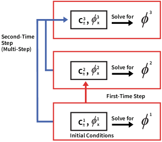
Figure 3: The initial value $\phi_{x}(1,0)$ is denoted $\phi_{x}^{1}$ and $\phi_{x}^{n}$ denotes the approximation of $\phi_{x}(1,t^{n})$. The initial data $c_{\pm}(x,0)$ is discretized resulting in initial vectors $\mathbf{c}_{+}^{1},\,\mathbf{c}_{-}^{1}\in\mathbb{R}^{N}$. Given $\mathbf{c}^{1}_{\pm}$ and $\phi_{x}^{1}$, we solve the elliptic PDE to determine $\boldsymbol{\phi}^{1}\in\mathbb{R}^{N}$. Using the one-step semi-implicit scheme (13) on the parabolic PDEs (1) and the ODE (10), we determine $\mathbf{c}_{\pm}^{2}$ and $\phi_{x}^{2}$. Given $\mathbf{c}^{2}_{\pm}$ and $\phi_{x}^{2}$, we solve the elliptic PDE to determine $\boldsymbol{\phi}^{2}$. (11) or (12) is then applied to determine $\mathbf{c}_{\pm}^{3}$ and $\phi_{x}^{3}$; $\boldsymbol{\phi}^{3}$ is then solved for, using $\mathbf{c}_{\pm}^{3}$ and $\phi_{x}^{3}$. And so forth.

Figure 3 presents this splitting scheme for the first and second (and subsequent) time-steps. It is important that $\boldsymbol{\phi}^{n+1}$ be solved for using $\mathbf{c}^{n+1}_{\pm}$ and $\phi_{x}^{n+1}$; not doing so reduces the global truncation error from $O(dt^{2})$ to $O(dt)$. Furthermore, because $\boldsymbol{\phi}^{n}$ at time $t^{n}$ is determined from the other quantities at time $t^{n}$, the elliptic equation does not factor into the computation of the approximate local truncation error during adaptive time-stepping.

2.5.2 Using the Fully-implicit Schemes BDF2 and VSBDF2

If fully-implicit time-stepping is used, the problem is viewed as a system of DAEs. If there is an imposed voltage, the $3N$ unknowns $\mathbf{c}_{+}^{n+1}$, $\mathbf{c}_{-}^{n+1}$, and $\boldsymbol{\phi}^{n+1}$ are simultaneously solved for. The parabolic PDEs (1) and the Butler-Volmer boundary conditions (4)–(5) are applied at time $t^{n+1}$; this results in $2N$ equations. The elliptic PDE (2) and its boundary conditions (8)–(9) are applied at time $t^{n+1}$ as well; this provides the additional $N$ equations.

The $3N$ equations are rewritten as $\mathcal{F}(\mathbf{c}_{+},\mathbf{c}_{-},\boldsymbol{\phi})=\vec{0}$ where $\mathcal{F}:\mathbb{R}^{3N}\to\mathbb{R}^{3N}$. The function $\mathcal{F}$ depends on the known quantities $\mathbf{c}_{\pm}^{n}$, $\boldsymbol{\phi}^{n}$, $\mathbf{c}_{\pm}^{n-1}$, and $\boldsymbol{\phi}^{n-1}$. We use two methods of finding approximate solutions. The first is a hand-coded Newton-Raphson method, for which iterations were stopped when $\|\mathcal{F}(\mathbf{c}_{+},\mathbf{c}_{-},\boldsymbol{\phi})\|<10^{-10}$. The second is MATLAB’s fsolve routine, which, by default, uses a trust region optimization algorithm. The results in Section 3.4 show that MATLAB’s fsolve is the faster and more stable method (as one would expect).

If there is an imposed current, rather than an imposed voltage, then $\phi_{x}^{n+1}$ is also solved for, resulting in $3N+1$ unknowns. The additional equation in the system of DAEs is (10) .

3 Simulations of the PNP-FBV Equations

Table 1 presents the results from convergence testing performed on the PNP-FBV system using both the SBDF2 and BDF2 numerical schemes. For these convergence tests, we considered current, rather than voltage boundary conditions, which requires time-stepping the additional ODE (10). The results demonstrate that both schemes are second-order accurate when the “ghost point” implementation of the boundary conditions (26) is used and that using the “direct” method (24) causes a loss of an order of accuracy.

$dt$	SBDF2, direct	SBDF2, ghost	BDF2
$5\times 10^{-7}$	1.9509	3.9904	3.9967
$5/2\times 10^{-7}$	1.9758	3.9952	3.9983
$5/4\times 10^{-7}$	1.9880	3.9976	3.9992
$5/8\times 10^{-7}$	1.9940	3.9988	3.9996
$5/16\times 10^{-7}$	1.9970	3.9993	3.9998

Table 1: Convergence tests on PNP-FBV system (1)–(9) with current boundary conditions (10) and an imposed external current $j_{\text{ext}}=0.5$. All model parameters were set to $1$ except $\epsilon=0.01$. For each method, we compute seven solutions on a uniform mesh $dx=1/30$ up to time $T=10^{-5}$, using equation (13) for the first time-step of the SBDF2 scheme and equation (16) for the first time-step of the BDF2 scheme. The SBDF2 scheme is implemented using both direct boundary conditions (24) and the ghost point approach (26). The i${}^{\text{th}}$ solution, denoted $\mathbf{u}_{i}=[\mathbf{c}_{+,i};\mathbf{c}_{-,i};\phi_{x,i}^{n+1}]$, is computed using $dt=1/2^{i}\times 10^{-6}$. That is $\mathbf{u}_{i}\in\mathbb{R}^{2(N+1)+1}\times\mathbb{R}^{n_{i}}$ where $n_{i}=10\times 2^{i}+1$ and $\mathbf{u}_{i}^{n_{i}}\in\mathbb{R}^{2(N+1)+1}$ approximates the solution at the final time $T$. The discrete solutions $\mathbf{u}_{i}$ at the final time $T=10^{-5}$ are used to define the ratios: $\|\mathbf{u}^{n_{i}}_{i}-\mathbf{u}^{n_{i+1}}_{i+1}\|/\|\mathbf{u}^{n_{i+1}}_{i+1}-\mathbf{u}^{n_{i+2}}_{i+2}\|$ with the $l^{2}$ norm. Ratios approaching 4 indicate global second-order accuracy in time. While we only show 5 values of $dt$ in the table, runs with $dt=5/32\times 10^{-7}$ and $dt=5/64\times 10^{-7}$ were necessary to create the ratios. Richardson extrapolation was not used.

We consider an initial value problem for the PNP-FBV system (1)–(9) with constant imposed voltage. Solutions are computed using both the (fully-implicit) VSBDF2 adaptive time-stepper and the (semi-implicit) VSSBDF2 adaptive time-stepper.

The plots to the left in Figure 1 present results from the simulations using the (fully-implicit) VSBDF2 adaptive time-stepper. The bottom plot demonstrates that the time-step increases until it reaches the user-specified $dt_{\text{max}}$; the time-step remains at this value for the duration of the simulation. The middle plot demonstrates that the (approximate) local truncation error stays within the user-specified range of $(tol-range,tol+range)$ until the time when the time-step reaches $dt_{\text{max}}$. Once the time-step stays at $dt_{\text{max}}$, the error control mechanism is no longer in play — the local truncation error begins to decay to around $10^{-11}$ and then stays around this value. Similarly, the top plot demonstrates that the norms of the deviation from the steady-state solution, $|\mathbf{c}^{n}_{\pm}-\mathbf{c}_{ss,\pm}|$ and $|\boldsymbol{\phi}^{n}-\boldsymbol{\phi}_{ss}|$, initially decreases exponentially fast, lingers around $10^{-7}$ for a bit, and then decreases to around $10^{-11}$. The deviations don’t decrease to $10^{-14}$ as they did for the SBDF2 simulation because the VSBDF2 adaptive time-stepper uses an iterative nonlinear solver and this solver is only solving the equations up to a tolerance of about $10^{-11}$.

The behaviour observed in the plots on the left is what one would expect for a numerically stable scheme that is computing a solution that is converging to an asymptotically stable steady-state solution. This expected behaviour is not what is observed when using the (semi-implicit) VSSBDF2 adaptive time-stepper.

The top figure on the right demonstrates that the solution found by the (semi-implicit) VSSBDF2 adaptive time-stepper initially decays towards the numerical steady-state solution. However, once the solution is within (approximately) $10^{-7}$ of the steady-state solution, this convergence ends and the computed solution stays about $10^{-7}$ away from the steady-state solution. (We note that if we decrease $tol$ then the deviation decreases further before “stalling out”.) The middle figure on the right demonstrates that the VSSBDF2 adaptive time-stepper is keeping the (approximate) local truncation error (17) within the user-specified range of $(tol-range,tol+range)$, as required as long as $dt_{\text{min}}<dt<dt_{\text{max}}$. The bottom figure on the right demonstrates that the time-step size initially increases exponentially fast and after a while it stabilizes; we denote the value that it stabilizes to as $dt_{\infty}$. To approximate it, we average 100 sequential time-steps at the end of the period of constant voltage/current.

The dashed line in the bottom figure on the left is the stability restriction found by the linear stability analysis presented in Section 5 of the companion article [1]; we denote this value as $dt^{*}$. This simulation demonstrates that the VSSBDF2 adaptive time-stepper appears to stabilize at a time-step size $dt_{\infty}$ that is precisely the stability restriction $dt^{*}$.

An example of an adaptive SBDF2 time-stepping scheme can be found in Rosam, Jimack and Mullis [47] use an adaptive SBDF2 time-stepping scheme to study a problem in binary alloy solidification. In their Figure 4, they appear to show time-steps relaxing to a constant value (i.e. stabilizing), but its cause is not given: they report that it is related to the tolerance set in the adaptive time-stepper. We find that our $dt_{\infty}$ is not affected by the tolerance parameter $tol$.

When using the (fully-implicit) VSBDF2 scheme, one can either extrapolate boundary conditions forward in time or they can be part of the nonlinear DAE system that has to be solved. We find that if we extrapolate the coupled boundary conditions of the elliptic PDE then this introduces a stability restriction on the time step size. That is, the observed behaviour of the solution is no longer like that shown in the left plots of Figure 1, rather it becomes like that shown in the right plots. This is in contrast to [58], where the authors time step a nonlinear diffusion equation using BDF methods. However they extrapolate the diffusivity coefficient forward in time to avoid the need for a nonlinear solve, but find that their time-stepper remains unconditionally stable.

3.1 Parameter choice and observed numerical behaviour

In all of our simulations using the (semi-implicit) VSSBDF2 adaptive time-stepper, we find that if there was a sufficiently long period of time during which either the voltage or the current were held constant then the solution would “come close to but not converge to” the corresponding steady-state solution (as in the top right plot of Figure 1) and the time-step sizes would stabilize to a limiting value $dt_{\infty}$ (as in the bottom right plot of Figure 1). We find that $dt_{\infty}$ depends on the imposed constant voltage (or on the imposed constant current) and that it does not depend on the parameters $tol$ and $range$ in the adaptive time-stepper.

In the companion article [1] we perform a linear stability analysis of the SBDF2 scheme about the steady-state solution, and demonstrate that the scheme is conditionally stable with a step size stability restriction $dt^{*}$. As suggested in the bottom right plot of Figure 1, and more thoroughly studied in [1], the $dt_{\infty}$ found by the VSSBDF2 adaptive time-stepper coincides with $dt^{*}$.

When computing solutions of the PNP-FBV system with time-independent voltage or current, we find that if we use the SBDF2 time-stepper with (fixed) $dt>dt^{*}$ then, after a transient, the computed solutions grow exponentially fast. If we use a (fixed) $dt<dt^{*}$ then, after a transient, the solution eventually converges exponentially fast to the steady-state solution and the local truncation error decays exponentially fast to zero (round-off). This is how we compute the steady-state solution that is used in computing the deviations from the steady-state solution presented in Figure 1.

If we use the (semi-implicit) VSSBDF2 adaptive time-stepper then one of two things happens. If $dt_{\text{max}}<dt^{*}$ then as the solution starts to converge to the steady-state solution $dt$ increases to $dt_{\text{max}}$. After this happens the local truncation error converges to zero and the solution converges to the steady-state solution. Alternatively, if $dt_{\text{max}}\geq dt^{*}$ then the solution starts to converge to the steady-state solution. As a result of this, the time-steps need grow in order to keep the local truncation error greater than $tol-range$ (which has been chosen to be positive). Once the time-step size increases past $dt^{*}$, the unstable eigenmode(s) of the underlying linearized problem start to grow exponentially and this growth stops the solution from converging to the steady-state solution. This growth causes the local truncation error to exceed $tol+range$, causing the adaptive time-stepper to decrease the time-step size. The net effect is that the adaptive time-stepper stabilizes its time-steps at $dt^{*}$ in order to keep the local truncation error in the user-specified interval [1].

3.2 Response to Time-dependent Forcing

We next considered the PNP-FBV system with time-dependent imposed voltage. The top plot of Figure 4 shows the imposed voltage: essentially a step function with a fast transition at $t=10$.

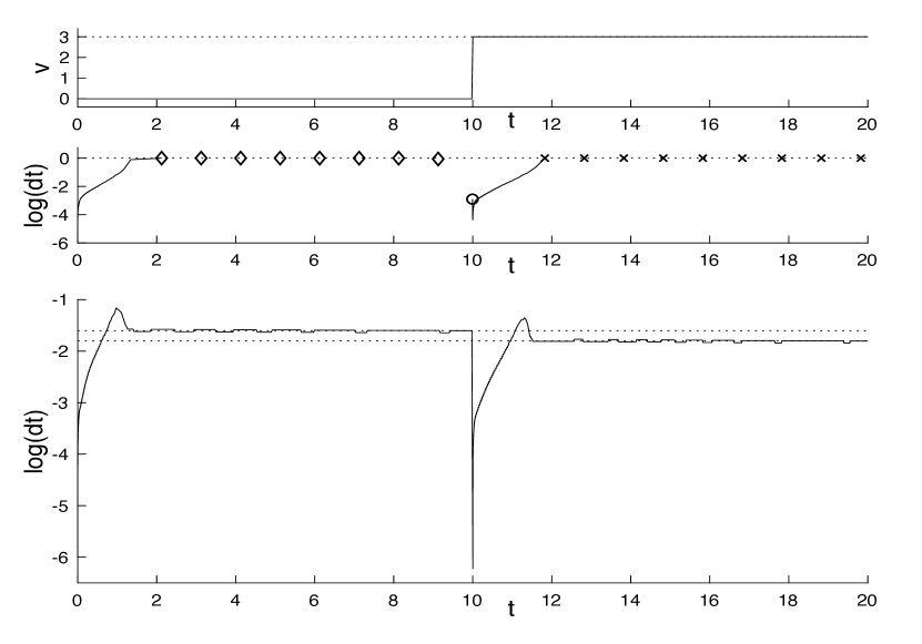
Figure 4: PNP-FBV system (1)–(9) with all physical parameters set to $1$ except $\epsilon=0.5$. A uniform mesh is used: $N=90$ and $L_{1}=L_{2}=L_{3}=1/3$. The initial data for the concentrations is $c_{\pm}(x,0)=1+.1\,\sin(2\pi x)$. Top plot: The imposed time-dependent voltage $v(t)$ has a sharp transition from 0 to 3 at time $t=10$, modeled by the equation $v(t)=3(\tanh(1000(t-10))+1)/2$. Middle plot: The time steps as a function of time for the fully-implicit scheme (solid line) and the semi-implicit scheme (dashed line). The diamond and x-marks indicate time-steps that are within 95% of the user-specified maximum value $dt_{\text{max}}$. The circle denotes the first time-step size after the last diamond-marked time step. Bottom plot: The time steps as a function of time for the semi-implicit scheme (solid line) and the fully-implicit scheme (dashed line). The dotted lines in the center and right figures correspond to $dt^{*}=0.0250$ and $0.0158$; they are the stability restrictions found using the linear stability analysis presented in Section 4 of the companion paper.

The middle plot of Figure 4 presents the time-steps chosen by the (fully-implicit) VSBDF2 adaptive time-stepper. In the first half of the simulation, the solution is converging to the $v=0$ steady-state solution. During this time, the time-steps coarsen until they reach the user-specified maximum time-step size: $dt_{\text{max}}=1$. See the diamond-marked times. The time-step refines markedly in response to the change in imposed voltage; the open circle indicates the first time-step size after the last diamond-marked time-step size. After the voltage step, the solution is converging to the $v=3$ steady-state solution. Again, the time-steps coarsen until they reach $dt_{\text{max}}$ (see the x-marks in the plot). The deviation of the solution from the steady-state solution and the behaviour of the local truncation error are the analogues of that shown in plots on the left of Figure 1.

The bottom plot of Figure 4 presents the time-steps chosen by the (semi-implicit) VSSBDF2 adaptive time-stepper. As discussed for the plots in the left of Figure 1, the solution starts to converge to the $v=0$ steady-state solution and the time-step size start to coarsen, stabilizing to a value $dt_{\infty}$. The time-step refine in response to the change in the imposed voltage after which the solution starts to converge to the $v=3$ steady-state solution and the time-step size start to coarsen, stabilizing to a different value $dt_{\infty}$. The two values of $dt_{\infty}$ coincide with the stability restrictions $dt^{*}$ found for the $v=0$ and $v=3$ steady-state solutions [1].

3.3 Effect of the Singular Perturbation Parameter

Next, we consider the singular perturbation parameter, $\epsilon$, which controls the dynamics of the boundary layers near the electrodes in the PNP-FBV system (2). Figure 5 presents some steady-state solutions for PNP-FBV system (1)–(9) with current boundary conditions (10) as computed using the SBDF2 scheme. The plots on the left present the steady-state concentrations, $c_{+,ss}(x)$ and $c_{-,ss}(x)$, for three values of $\epsilon$. The smaller the value of $\epsilon$, the thinner the transition layer near $x=0$ and $x=1$ is. The plots on the right present the corresponding steady-state potential, $\phi_{ss}(x)$. The top left plot shows that, in the bulk, $c_{+,ss}$ and $c_{-,ss}$ are very close in value (the system is nearly electroneutral). We find that, for small values of $\epsilon$, $c_{+,ss}(x)-c_{-,ss}(x)\approx\epsilon^{2}\,C(x)$ in the bulk. This is the reason why the steady-state potential is not linear in the bulk (see the top right plot); in the bulk, it satisfies $\phi_{xx}=C/2$.

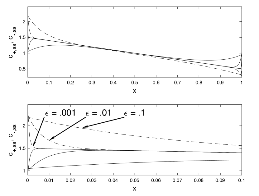
(a)

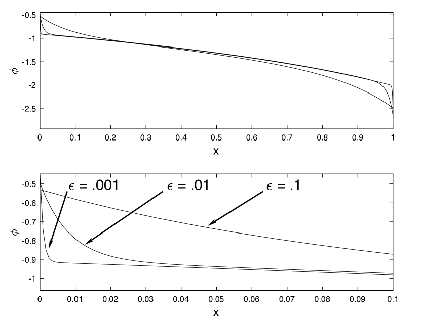
(b)

Figure 5: Steady-state solutions for PNP-FBV system (1)–(9) with current boundary conditions (10). The imposed external current is constant $j_{\text{ext}}(t)=0.5$. The simulations were run until time $t=5$; the profiles at that time are shown here. All physical parameters were set to $1$, except for $\epsilon$. For $\epsilon=0.1$, a uniform-in-space mesh was used with $dx=1/90$. For $\epsilon=0.01$, a piecewise uniform-in-space mesh was used with $dx=1/600$ in $[0,0.1]$ and $[0.9,1]$ and $dx=1/75$ in $[0.1,0.9]$. For $\epsilon=0.001$, a piecewise uniform-in-space mesh was used with $dx=1/1200$ in $[0,0.05]$ and $[0.95,1]$ and $dx=3/100$ in $[0.05,0.95]$. Left plot: concentrations $c_{+,ss}$ (solid) and $c_{-,ss}$ (dashed), versus $x$. Right plot: potential, $\phi_{ss}$, versus $x$.

For relatively small values of $\epsilon$, we find that if one decreases $\epsilon$ by a factor of $a$ then the limiting time-step size of the (semi-implicit) VSSBDF2 adaptive time-stepper, $dt_{\infty}$, decreases by roughly $a^{2}$; see Table 2. A detailed discussion of this effect can be found in the companion article [1].

$\epsilon$	$dt_{\infty}$	$dt_{\infty}/\epsilon^{2}$
$0.1$	$0.0257$	$2.57$
$0.01$	$0.000241$	$2.41$
$0.001$	$3.70\times 10^{-6}$	$3.70$
$10^{-4}$	$2.48\times 10^{-8}$	$2.48$
$10^{-5}$	$2.25\times 10^{-10}$	$2.25$
$10^{-6}$	$2.37\times 10^{-12}$	$2.37$

Table 2: The PNP-FBV system (1)–(9) are simulated with the imposed voltage $v(t)=0$. All physical parameters were set to $1$, except for $\epsilon$. Six values of $\epsilon$ are considered. We denote the limiting timestep size found by the VSSBDF2 adaptive time-stepper by $dt_{\infty}$. $dt_{\infty}$ was computed by averaging the time-step sizes over 100 sequential time-steps chosen late in the simulation.

By taking small enough time-steps, the (semi-implicit) VSSBDF2 adaptive time-stepper is able to run with small values of $\epsilon$. Furthermore, although it is more computationally expensive, the (fully-implicit) VSBDF2 adaptive time-stepper is able to take arbitrarily large time-steps for equilibrated solutions, regardless of the value of $\epsilon$.

3.4 Comparison Between Semi-implicit and Fully-Implicit Methods

As demonstrated in Table 2, the stability restriction on the time-step size for VSSBDF2 is roughly on the order of $\epsilon^{2}$ as $\epsilon\to 0$, whereas there is no dependence on $\epsilon$ on the step size for VSBDF2. This implies that there will be a break-even point: in some regimes the VSSBDF2 scheme will be faster, while in other regimes the VSBDF2 scheme will be faster despite being significantly slower per time-step.

To compare the two schemes, we repeated the experiments in Table 2, using Matlab’s profiler to measure performance time, and keeping track of the number of iterations and the average time step size for our simulations. See Table 3. “Total iterations” counts the number of coarse-step-fine-step sequences taken, including those taken while seeking an acceptable time-step size (see Algorithm 1). “Time steps” counts the number of times the time index is actually incremented. When using VSBDF2, we tested two methods of solving the system of nonlinear equations: Newton’s method, and Matlab’s fsolve. We ran all simulations to a final time $t_{\text{end}}=1$. We did not run with values of $\epsilon$ smaller than $10^{-4}$ because the VSSBDF2 code would have taken over fifteen hours. Also, our Newton-Raphson method code ran into conditioning issues for $\epsilon=10^{-4}$ although Matlab’s fsolve did not.

$\epsilon$	Performance time (s)	Total iterations (including error control iterations)	Time steps	Average time step
	(semi-implicit) VSSBDF2
0.1	0.661	625	445	2.21E-03
0.01	5.524	7836	7614	1.31E-04
0.001	552.675	788026	754002	1.23E-06
10-4	>15 hours
	(fully-implicit) VSBDF2, Newton solver
0.1	201.201	530	356	3.15E-03
0.01	214.671	525	354	2.86E-03
0.001	255.329	530	355	3.16E-03
10-4	Unable to run, Jacobian poorly conditioned
	(fully-implicit) VSBDF2, fsolve solver
0.1	157.09	530	356	3.17E-03
0.01	153.099	525	354	2.86E-03
0.001	158.584	530	355	3.16E-03
10-4	157.031	526	355	2.86E-03

Table 3: Profiling results on the (semi-implicit) VSSBDF2 and (fully-implicit) VSBDF2 adaptive time-steppers. For the fully-implicit method two nonlinear solvers were compared: a simple Newton method and Matlab’s fsolve routine. Parameter values are identical to the ones used for Table 2, except all experiments were run to a final time $t_{\text{end}}=1$. Performance time was obtained using Matlab’s profiler. “Total iterations” counts number of coarse-step-fine-step sequences taken, including those taken while seeking an acceptable time-step size (see Algorithm 1), whereas “Time steps” counts the number of times the time index is actually incremented.

The profiling results show a clear trend: with decreasing $\epsilon$, the semi-implicit scheme’s number of time steps increases rapidly, while the fully-implicit scheme’s number of time steps remains constant. This is due to the semi-implicit scheme’s time step stability restriction, which depends on $\epsilon$. This shows that, for this particular set of parameters and with no forcing, the semi-implicit scheme is favorable when $\epsilon$ is roughly greater than $0.001$, and the fully-implicit scheme is favorable when $\epsilon<0.001$. In other parameter and forcing regimes, the “break-even” value of $\epsilon$ will be different. We note that the test has been run in a situation where the solution equilibrates. One does this when seeking steady-state solutions, for example. The final time $t_{\text{end}}$ is another user-specified parameter that affects the “break-even” value of $\epsilon$.

4 Conclusions and Future Work

In this work, we considered the Poisson-Nernst-Planck equations with generalized Frumkin-Butler-Volmer reaction kinetics at the electrodes. We developed a solver that dynamically chooses the time-step size so that the local truncation error is within user-specified bounds; this is a novel contribution to the solution of the PNP equations. The spatial discretization can be nonuniform, allowing for the finer mesh needed near the electrodes to resolve the boundary layers. Adaptive time-stepping allows the solver to choose small time-steps during the initial transient period during which the boundary layers may be forming quickly in response to the boundary conditions, and also allows one to more efficiently study physical situations in which the imposed voltage or current have sudden, fast changes.

We considered two adaptive time-stepping schemes in this work. The (semi-implicit) VSSBDF2 adaptive time-stepper was shown to have a stability restriction which causes its time-step sizes to stabilize to a limiting value, $dt_{\infty}$, in the long-time limit of constant voltage or current, whereas the (fully-implicit) VSBDF2 adaptive time-stepper was found to have no restriction on the time step beyond the user-specified $dt_{\text{max}}$. However, the fully-implicit time-stepper requires a computationally expensive nonlinear solve per step, resulting in longer computation time per time step. The cause of the limiting time-step, $dt_{\infty}$, found by the (semi-implicit) VSSBDF2 adaptive time-stepper can be understood by linearizing the SBDF2 scheme about the steady-state solution and is fully explored in the companion article [1].

We found that $dt_{\infty}$ is $\epsilon$-dependent. As a result, the (semi-implicit) VSSBDF2 adaptive time-stepper is favoured for larger values of $\epsilon$ and the (fully-implicit) VSBDF2 adaptive time-stepper is favoured for smaller values.

Appendix A Derivation of the Local Truncation Error Formula and the Extrapolation Formula

In this appendix, the error approximation and extrapolation formula used in Subsection 2.2 are derived. We consider time-stepping the ODE ${du}/{dt}=f(u)+g(u)$ where the value of $u$ at time $n+1$ is given by (12). Making the substitutions $u^{n+1}=u(t+dt_{\text{now}})$ and $u^{n-1}=u(t-dt_{\text{old}})$ and performing a multivariable Taylor expansion about $t$, the local truncation error is found to take the form

$$LTE =\left(u^{\prime}(t)-f(u(t))-g(u(t))\right)dt_{\text{now}}+\left(u^{\prime\prime}(t)-f^{\prime}(u(t))\,u^{\prime}(t)-g^{\prime}(u(t))\,u^{\prime}(t)\right)dt_{\text{now}}^{2}$$

$$\hskip 36.135pt+\left(\frac{1}{2}f^{\prime\prime}(u(t))\,u^{\prime}(t)^{2}+\frac{1}{2}f^{\prime}(u(t))\,u^{\prime\prime}(t)-\frac{1}{6}u^{(3)}(t))\right)dt_{\text{old}}\,dt_{\text{now}}^{2}$$

$$\hskip 36.135pt+\left(-\frac{1}{2}g^{\prime\prime}(u(t))\,u^{\prime}(t)^{2}-\frac{1}{2}g^{\prime}(u(t))\,u^{\prime\prime}(t)+\frac{1}{3}u^{(3)}(t)\right)dt_{\text{now}}^{3}+O(dt^{4})$$ (27)

where $O(dt^{4})$ denotes terms where $dt_{\text{now}}$ and $dt_{\text{old}}$ combined appear four or more times. If $u(t)$ is a thrice-differentiable solution of the ODE, the $dt_{\text{now}}$ and $dt_{\text{now}}^{2}$ terms vanish and the cubic term can be simplified:

$$LTE =\left(\frac{1}{2}f^{\prime\prime}(u(t))\,u^{\prime}(t)^{2}+\frac{1}{2}f^{\prime}(u(t))\,u^{\prime\prime}(t)-\frac{1}{6}u^{(3)}(t)\right)dt_{\text{old}}dt_{\text{now}}^{2}$$

$$\hskip 54.2025pt+\left(-\frac{1}{2}g^{\prime\prime}(u(t))\,u^{\prime}(t)^{2}-\frac{1}{2}g^{\prime}(u(t))u^{\prime\prime}(t)+\frac{1}{3}u^{(3)}(t)\right)dt_{\text{now}}^{3}+O(dt^{4})$$ (28)

$$=\left(\frac{1}{3}u^{(3)}(t)-\frac{1}{2}g^{\prime\prime}(u(t))\,u^{\prime}(t)^{2}-\frac{1}{2}g^{\prime}(u(t))\,u^{\prime\prime}(t)\right)dt_{\text{now}}^{2}\left(dt_{\text{now}}+dt_{\text{old}}\right)+O(dt^{4}).$$ (29)

This means that if $u^{(3)}(t)$ is bounded, the local truncation error for the coarse step is

$$\epsilon_{c}=u_{c}^{n+1}-u(t^{n+1})\approx Cdt_{\text{now}}^{2}\left(dt_{\text{now}}+dt_{\text{old}}\right)$$ (30)

To find the local truncation error for $u_{f}^{n+1}$, we find the local truncation error for $u_{f}^{n+\frac{1}{2}}$ by replacing $dt_{\text{now}}$ and $dt_{\text{old}}$ in (30) by $\frac{dt_{\text{now}}}{2}$ and $\frac{dt_{\text{old}}}{2}$, respectively. We then find the local truncation error for $u_{f}^{n+1}$ by setting both $dt_{\text{now}}$ and $dt_{\text{old}}$ to $\frac{dt_{\text{now}}}{2}$. Adding these local truncation errors yields the LTE for $u_{f}^{n+1}$,

$$\epsilon_{f}=u_{f}^{n+1}-u(t^{n+1})\approx\frac{Cdt_{\text{now}}^{2}\left(dt_{\text{now}}+dt_{\text{old}}\right)}{8}+C\,\frac{dt_{\text{now}}^{3}}{4}$$ (31)

Using equations (30) and (31), we can approximate $C$ using $u_{c}$, $u_{f}$, $dt_{\text{now}}$ and $dt_{\text{old}}$ and then use this approximation in (30), resulting in

$$\epsilon_{c}\approx\frac{u_{c}-u_{f}}{\frac{5}{8}dt_{\text{now}}^{3}+\frac{7}{8}dt_{\text{now}}^{2}dt_{\text{old}}}\;dt_{\text{now}}^{2}\left(dt_{\text{now}}+dt_{\text{old}}\right)$$ (32)

Finally, we subtract $\epsilon_{c}$ from $u_{c}^{n+1}$ to create a more accurate approximation of $u(t^{n+1})$. This results in the extrapolation formula $u(t^{n+1})\approx u_{c}^{n+1}-\epsilon_{c}=\alpha u^{n+1}_{c}+\beta u^{n+1}_{f}$ where

$$\alpha=-\frac{dt_{\text{old}}+3\,dt_{\text{now}}}{7\,dt_{\text{old}}+5\,dt_{\text{now}}},\;\;\;\beta=8\,\frac{dt_{\text{old}}+dt_{\text{now}}}{7\,dt_{\text{old}}+5\,dt_{\text{now}}}.$$ (33)

We note that if the time-stepping scheme is fully-implicit, this corresponds to setting $f(u)=0$ in equation (33). In this case, (29) is replaced by

$$LTE=-\frac{1}{6}\left(g^{\prime\prime}(u(t))\,u^{\prime}(t)^{2}+g^{\prime}(u(t))\,u^{\prime\prime}(t)\right)dt_{\text{now}}^{2}\left(dt_{\text{now}}+dt_{\text{old}}\right)+O(dt^{4})$$

but there are no resulting changes to equations (30)–(33).

Appendix B Acknowledgements

Research supported in part by NSERC grant OGP06617.

We thank Greg Lewis, Steven Ruuth, and Adam Stinchcombe for helpful conversations and encouragement.

References

- [1] Mary C. Pugh, David Yan, and Francis P. Dawson. A study of the numerical stability of an imex scheme with application to the Poisson-Nernst-Planck equations. arXiv:1905.01368, 2020.
- [2] P.M. Biesheuvel and M.Z. Bazant. Nonlinear dynamics of capacitive charging and desalination by porous electrodes. Phys. Rev. E, 81(3):031502, 2010.
- [3] P.M. Biesheuvel, Yeqing Fu, and M.Z. Bazant. Diffuse charge and Faradaic reactions in porous electrodes. Phys. Rev. E, 83(6):061507, 2011.
- [4] P.M. Biesheuvel, Yeqing Fu, and M.Z. Bazant. Electrochemistry and capacitive charging of porous electrodes in asymmetric multicomponent electrolytes. Russ. J. Electrochem., 48(6):580–591, 2012.
- [5] P.B. Peters, R. van Roij, Martin Z. Bazant, and P.M. Biesheuvel. Analysis of electrolyte transport through charged nanopores. Phys. Rev. E, 93:053108, 2016.
- [6] Ian Streeter and Richard G. Compton. Numerical simulation of potential step chronoamperometry at low concentrations of supporting electrolyte. J. Phys. Chem. C, 112(35):13716–13728, 2008.
- [7] Richard G. Compton and Craig E. Banks. Understanding Voltammetry. Imperial College Press, London, 2011.
- [8] E. Victoria Dydek and Martin Z. Bazant. Nonlinear dynamics of ion concentration polarization in porous media: The leaky membrane model. AlChE Journal, 59(9):3539–3555, 2013.
- [9] Victor V. Nikonenko, Natalia D. Pismenskaya, Elena I. Belova, Philippe Sistat, Patrice Huguet, Gérald Pourcelly, and Christian Larchet. Intensive current transfer in membrane systems: Modelling, mechanisms and application in electrodialysis. Adv. Colloid Interface Sci., 160(1):101–123, 2010.
- [10] A. Yaroshchuk. Over-limiting currents and deionization shocks in current-induced polarization: local equilibrium analysis. Adv. Colloid Interface Sci., 183:68–81, 2012.
- [11] Martin Z. Bazant and Todd M. Squires. Induced-charge electrokinetic phenomena. Curr. Opin. Colloid Interface Sci., 15(3):203–213, 2010.
- [12] Martin Z. Bazant, Mustafa Sabri Kilic, Brian D. Storey, and Armand Ajdari. Towards an understanding of induced-charge electrokinetics at large applied voltages in concentrated solutions. Adv. Colloid Interface Sci., 152(1):48–88, 2009.
- [13] Martin Z. Bazant, Brian D. Storey, and Alexei A. Kornyshev. Double layer in ionic liquids: Overscreening versus crowding. Phys. Rev. Lett., 106(4):046102, 2011.
- [14] Alexei A. Kornyshev. Double-layer in ionic liquids: Paradigm change? J. Phys. Chem. B, 111:5545–5557, 2007.
- [15] Martin Z. Bazant, Kevin T. Chu, and B.J. Bayly. Current-voltage relations for electrochemical thin films. SIAM J. Appl. Math., 65(5):1463–1484, 2005.
- [16] Kevin T. Chu and Martin Z. Bazant. Electrochemical thin films at and above the classical limiting current. SIAM J. Appl. Math., 65(5):1485–1505, 2005.
- [17] P.M. Biesheuvel, M. van Soestbergen, and M.Z. Bazant. Imposed currents in galvanic cells. Electrochim. Acta, 54:4857–4871, 2009.
- [18] P. Maarten Biesheuvel, Alejandro A. Franco, and Martin Z. Bazant. Diffuse charge effects in fuel cell membranes. J. Electrochem. Soc., 156(2):B225–B233, 2009.
- [19] Alpha A Lee, Svyatoslav Kondrat, Gleb Oshanin, and Alexei A Kornyshev. Charging dynamics of supercapacitors with narrow cylindrical nanopores. Nanotechnology, 25(31):315401, 2014.
- [20] David Yan, Martin Z. Bazant, P.M. Biesheuvel, Mary C. Pugh, and Francis P. Dawson. Theory of linear sweep voltammetry with diffuse charge: Unsupported electrolytes, thin films, and leaky membranes. Phys. Rev. E, 95:033303, Mar 2017.
- [21] Martin Z. Bazant. Theory of chemical kinetics and charge transfer based on nonequilibrium thermodynamics. Accounts Chem. Res., 46(5):1144–1160, 2013.
- [22] M. van Soestbergen. Frumkin-Butler-Volmer theory and mass transfer in electrochemical cells. Russ. J. Electrochem., 48(6):570–579, 2012.
- [23] A.A. Moya, J. Castilla, and J. Horno. Ionic transport in electrochemical cells including electrical double-layer effects. A network thermodynamics approach. J. Phys. Chem., 99:1292–1298, 1995.
- [24] M. van Soestbergen, P.M. Biesheuvel, and M.Z. Bazant. Diffuse-charge effects on the transient response of electrochemical cells. Phys. Rev. E, 81(2):1–13, 2010.
- [25] Allen J. Bard and Larry R. Faulkner. Electrochemical Methods: Fundamentals and Applications. John Wiley & Sons, New York, 2001.
- [26] John Newman and Karen E. Thomas-Alyea. Electrochemical Systems. John Wiley & Sons, Hoboken, NJ, 2012.
- [27] David Yan. Macroscopic Modeling of a One-Dimensional Electrochemical Cell Using the Poisson-Nernst-Planck Equations. PhD thesis, University of Toronto, 2017.
- [28] John Newman and William H. Smyrl. The polarized diffuse double layer. Trans. Faraday Soc., 61:2229–2237, 1965.
- [29] William H. Smyrl and John Newman. Double layer structure at the limiting current. Trans. Faraday Soc., 63:207–216, 1966.
- [30] Martin Z. Bazant, Katsuyo Thornton, and Armand Ajdari. Diffuse-charge dynamics in electrochemical systems. Phys. Rev. E, 70(2):021506, 2004.
- [31] John O’M. Bockris and Amulya Reddy. Modern Electrochemistry 1: Ionics. Springer US, Boston, MA, 2002.
- [32] H. Cohen and J. W. Cooley. The numerical solution of the time-dependent Nernst-Planck equations. Biophys. J., 5(2):145–162, 1965.
- [33] James R. Sandifer and Richard P. Buck. An algorithm for simulation of transient and alternating current electrical properties of conducting membranes, junctions and one-dimensional, finite galvanic cells. J. Phys. Chem., 79(4):384–392, 1975.
- [34] Timothy R. Brumleve and Richard P. Buck. Numerical solution of the Nernst-Planck and Poisson equation system with applications to membrane electrochemistry and solid state physics. J. Electroanal. Chem., 90(1):1–31, 1978.
- [35] Tomasz Sokalski, Peter Lingenfelter, and Andrzej Lewenstam. Numerical solution of the coupled Nernst-Planck and Poisson equations for liquid junction and ion selective membrane potentials. J. Phys. Chem. B, 107(11):2443–2452, 2003.
- [36] W. D. Murphy, J. A. Manzanares, S. Mafé, and H. Reiss. Numerical simulation of the nonequilibrium diffuse double layer in ion-exchange membranes. J. Phys. Chem., 97(32), 1993.
- [37] G.W. Gear. Numerical Initial Value Problems in Ordinary Differential Equations. Prentice Hall, Englewood Cliffs, NJ, 1971.
- [38] Donald L. Scharfetter and Herman K. Gummel. Large-signal analysis of a silicon read diode oscillator. IEEE Trans. Electron Devices, 16(1):64–77, 1969.
- [39] Silvano Erlicher, Luca Bonaventura, and Oreste S. Bursi. The analysis of the generalized-α method for non-linear dynamic problems. Comput. Mechanics, 28(2):83–104, 2002.
- [40] Dieter Britz and Jörg Strutwolf. Several ways to simulate time dependent liquid junction potentials by finite differences. Electrochim. Acta, 137:328–335, 2014.
- [41] Dieter Britz. Digital Simulation in Electrochemistry. Springer, Berlin, 2005.
- [42] Richard G. Compton, Eduardo Laborda, and Kristopher R. Ward. Understanding Voltammetry: Simulation of Electrode Processes. Imperial College Press, London, 2014.
- [43] D. Wang and S.J. Ruuth. Variable step-size implicit-explicit linear multistep methods for time-dependent partial differential equations. J. Comput. Math., 26(6):838–855, 2008.
- [44] O. Axelsson, X. He, and M. Neytcheva. Numerical solution of the time-dependent Navier-Stokes equation for variable density-variable viscosity. part I. Technical report, Uppsala University, 2014.
- [45] Daniel Lecoanet, Josiah Schwab, Eliot Quataert, Lars Bildsten, F.X. Timmes, Keaton J. Burns, Geoffrey M. Vasil, Jeffrey S. Oishi, and Benjamin P. Brown. Turbulent chemical diffusion in convectively bounded carbon flames. Astrophys. J., 832(1):71, 2016.
- [46] Gunilla Linde, Jonas Persson, and Lina Von Sydow. A highly accurate adaptive finite difference solver for the Black-Scholes equation. Int. J. Comp. Math., 86(12):2104–2121, 2009.
- [47] J. Rosam, P.K. Jimack, and A. Mullis. A fully implicit, fully adaptive time and space discretisation method for phase-field simulation of binary alloy solidification. J. Comput. Phys., 225(2):1271–1287, 2007.
- [48] S. Eckert, H. Baaser, D. Gross, and O. Scherf. A BDF2 integration method with step size control for elasto-plasticity. Comput. Mech., 34(5):377–386, 2004.
- [49] Laurits Højgaard Olesen, Martin Z. Bazant, and Henrik Bruus. Strongly nonlinear dynamics of electrolytes in large ac voltages. Phys. Rev. E, 82(1):011501, 2010.
- [50] Roger Peyret. Spectral Methods for Incompressible Viscous Flow. Springer-Verlag, New York, 2002.
- [51] Michel Crouzeix. Une méthode multipas implicite-explicite pour l’approximation des équations d’évolution paraboliques. Numer. Math., 35(3):257–276, 1980.
- [52] U.M. Ascher, S.J. Ruuth, and B.T.R. Wetton. Implicit-explicit methods for time-dependent partial differential equations. SIAM J. Numer. Anal., 32(3):797–823, 1995.
- [53] Ernst Hairer, Syvert P. Nørsett, and Gerhard Wanner. Solving Ordinary Differential Equations I: Nonstiff Problems (Springer Series In Computational Mathematics). Springer Berlin, Heidelberg, 2009.
- [54] Lloyd N. Trefethen. Approximation Theory and Approximation Practice. SIAM, 2013.
- [55] Rodrigo B. Platte and Lloyd N. Trefethen. Chebfun: a new kind of numerical computing. In Progress in Industrial Mathematics at ECMI 2008, pages 69–87, 2008.
- [56] David Yan, Mary C. Pugh, and Francis P. Dawson. A variable step size implicit-explicit scheme for the solution of the Poisson-Nernst-Planck equations. arXiv:1703.10297, 2017.
- [57] J.M. Thomas. Numerical Partial Differential Equations: Finite Difference Methods. Springer, New York, 1995.
- [58] Oscar P. Bruno and Edwin Jimenez. Higher-Order Linear-Time Unconditionally Stable Alternating Direction Implicit Methods for Nonlinear Convection-Diffusion Partial Differential Equation Systems. J. Fluids Eng.-Trans. ASME, 136(6), JUN 2014.