Small parameters in infrared quantum chromodynamics

Abstract

We study the long-distance properties of quantum chromodynamics in the Landau gauge in an expansion in powers of the three-gluon, four-gluon, and ghost-gluon couplings, but without expanding in the quark-gluon coupling. This is motivated by two observations. First, the gauge sector is well-described by perturbation theory in the context of a phenomenological model with a massive gluon. Second, the quark-gluon coupling is significantly larger than those in the gauge sector at large distances. In order to resum the contributions of the remaining infinite set of QED-like diagrams, we further expand the theory in $1/N_{c}$, where $N_{c}$ is the number of colors. At leading order, this double expansion leads to the well-known rainbow approximation for the quark propagator. We take advantage of the systematic expansion to get a renormalization-group improvement of the rainbow resummation. A simple numerical solution of the resulting coupled set of equations reproduces the phenomenology of the spontaneous chiral symmetry breaking: for sufficiently large quark-gluon coupling constant, the constituent quark mass saturates when its valence mass approaches zero. We find very good agreement with lattice data for the scalar part of the propagator and explain why the vectorial part is poorly reproduced.

I Introduction

The long-distance regime of quantum chromodynamics (QCD) is the arena of several important phenomena. Of utmost phenomenological relevance is the so-called spontaneous chiral symmetry breaking (S$\chi$SB), which is responsible for the dramatic increase of the running mass of the light quarks, from a few MeV to roughly a third of the nucleon mass, when the renormalization-group (RG) scale is lowered from a few GeV down to zero. This behavior is now clearly established by lattice simulations, see e.g. Bowman:2005vx ; Oliveira:2016muq , but its description within analytic approaches remains a difficult problem. Indeed, this requires one to control the theory in a regime where the couplings are large, or even undefined, if one trusts standard perturbation theory. In fact, it is widely believed that the whole infrared regime of QCD is nonperturbative in nature and that its properties can be accessed only through nonperturbative approaches, such as nonperturbative renormalization group (NPRG), Schwinger-Dyson (SD) equations, the Hamiltonian formalism or lattice simulations Schleifenbaum:2006bq ; Quandt:2013wna ; vonSmekal97 ; Alkofer00 ; Zwanziger01 ; Fischer03 ; Bloch03 ; Pawlowski:2003hq ; Fischer:2004uk ; Aguilar04 ; Boucaud06 ; Aguilar07 ; Aguilar08 ; Boucaud08 ; Fischer08 ; RodriguezQuintero10 ; Huber:2012kd ; Sternbeck:2007ug ; Cucchieri:2007rg ; Cucchieri:2008fc ; Sternbeck:2008mv ; Cucchieri:2009zt ; Bogolubsky:2009dc ; Dudal:2010tf .

On the analytical side, it is well understood that the physics of S$\chi$SB can be reproduced by retaining a certain family of diagrams, the so-called rainbow truncation (for classical references on the subject, see Refs. Johnson:1964da ; Maskawa:1974vs ; Maskawa:1975hx ; Miransky:1984ef ; Atkinson:1988mv ; Atkinson:1988mw ; Bhagwat:2004hn ; some recent reviews are Refs. Maris:2003vk ; Roberts:2007jh ). The corresponding truncation for two-body bound states, the so-called rainbow-ladder truncation, has been successfully applied to meson spectroscopy Maris:1999nt ; Eichmann:2008ae . This appears naturally as the first nontrivial contribution in some nonperturbative approximation schemes, e.g., based on $n$-particle-irreducible techniques Sanchis-Alepuz:2015tha ; Williams:2015cvx ; Eichmann:2016yit . Note, however, that S$\chi$SB requires a sufficiently large coupling, as was first pointed out by Nambu and Jona-Lasinio Nambu:1961tp ; Nambu:1961fr . Consequently, it remains unclear why the particular family of rainbow diagrams should be retained while some other diagrams are discarded. Moreover, some modeling is usually necessary for the gluon propagator and the quark-gluon vertex.

A clue in order to explain the success of the rainbow truncation may be the following. Recent works have shown that the dynamics in the gauge sector can be described by perturbative means within a massive deformation of the standard Landau gauge QCD Lagrangian Tissier:2010ts ; Tissier:2011ey ; Pelaez:2013cpa ; Reinosa:2017qtf . This is motivated by thorough studies of QCD correlation functions with lattice simulations, the solutions of truncated SD and NPRG equations, as well as variational methods in the Hamiltonian formalism Schleifenbaum:2006bq ; Quandt:2013wna ; vonSmekal97 ; Alkofer00 ; Zwanziger01 ; Fischer03 ; Bloch03 ; Pawlowski:2003hq ; Fischer:2004uk ; Aguilar04 ; Boucaud06 ; Aguilar07 ; Aguilar08 ; Boucaud08 ; Fischer08 ; RodriguezQuintero10 ; Huber:2012kd . In the Landau gauge, the gluon propagator displays a saturation at small momenta (the so-called decoupling — or massive — solution), while the ghost propagator presents a massless behaviour at vanishing momentum Sternbeck:2007ug ; Cucchieri:2007rg ; Cucchieri:2008fc ; Sternbeck:2008mv ; Cucchieri:2009zt ; Bogolubsky:2009dc ; Dudal:2010tf , as in the bare theory. The physical origin of this massive behavior for the gluons evades the usual perturbative treatment of the theory. However, there are strong evidences which indicate that this gluon mass is the major nonperturbative ingredient of the infrared regime of Yang-Mills theory (for a recent general discussion on the topic, see Reinosa:2017qtf ). Indeed, for what concerns pure Yang-Mills theories, it was shown in a series of articles Tissier:2010ts ; Tissier:2011ey ; Pelaez:2013cpa that one-loop calculations of two- and three-points correlation functions in a simple extension of the Landau gauge Faddeev-Popov Lagrangian by means of a (phenomenologically motivated) gluon mass compare quite well with lattice simulations, with a maximal error ranging from 10% to 20% depending on the correlation function. This is a particular case of the class of Curci-Ferrari (CF) Lagrangians Curci76 . This surprising result can be traced back to the fact that, within this phenomenological model, the interaction strength $\alpha_{S}$ remains moderate, even in the infrared regime, in agreement with lattice simulations.

Similar studies were also performed with dynamical quarks Pelaez:2014mxa ; Pelaez:2015tba : the gluon, ghost and quark propagators, as well as the quark-gluon correlation function were computed at one loop in the massive extension of Landau-gauge QCD. Most of the correlation functions that could be compared with lattice simulations showed the correct qualitative behaviors, with the noticeable exception of the vectorial part of the quark propagator. However, for small values of the bare quark masses, the quantitative comparison to lattice data was less convincing in the quark sector.

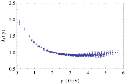
Figure 1: A measure of the relative of the quark-gluon and the ghost-gluon couplings. Figure generated from the lattice data of Ref. Skullerud:2003qu .

Again, lattice simulations give us an important clue for understanding this poorer results in presence of dynamical quarks Oliveira:2016muq ; Skullerud:2003qu . Indeed, although equal in the ultraviolet, the coupling constants of the different sectors of the theory differ significantly at long distances. Lattice simulations show that the coupling in the quark sector is two to three times larger in the infrared than the one in the gauge sector. This has also been observed in SD and NPRG contexts Aguilar:2014lha ; Braun:2014ata as well as in the one-loop calculation of the quark-guon vertex of Ref. Pelaez:2015tba . This is illustrated in Fig. 1, where we show the ratio between the quark-gluon and ghost-gluon vertices in some kinematical configuration. In this situation, a perturbative expansion in powers of the quark-gluon coupling is questionable (recall that the relevant expansion parameter is proportional to the square of the coupling). Note that the fact that the quark-gluon coupling must be larger than the one observed in the gluonic sector is also in line with phenonomenological considerations Roberts:2007jh : the coupling observed on the lattice in the gluonic sector is too small to trigger the S$\chi$SB.

In this article, we propose to extend the work of Pelaez:2014mxa ; Pelaez:2015tba by taking into account the above observations. We treat the couplings in the gauge sector perturbatively while keeping all orders of the quark-gluon coupling. At leading order, this reduces the set of diagrams to those appearing in an Abelian theory. We further use an expansion in the number of colors $N_{c}$ 'tHooft:1974hx to obtain closed expressions for the associated correlation functions (for a classical reference on the validity of the large-$N_{c}$ limit in QCD, see, for instance, Ref. Witten:1979kh ; for a recent numerical analysis of the question see, for instance, Ref. DeGrand:2016pur ). At leading order in $1/N_{c}$, this reduces to the rainbow-ladder diagrams.

This is most welcome since this set of diagrams is known to capture the physics of S$\chi$SB Johnson:1964da ; Maskawa:1974vs ; Maskawa:1975hx ; Miransky:1984ef ; Atkinson:1988mv ; Atkinson:1988mw ; Bhagwat:2004hn . The benefit of the present approach is that this approximation is obtained in a controlled expansion that can be, in principle, systematically improved. In particular, at leading order, the structure of the gluon propagator is determined by perturbation theory in the CF model. Moreover, this allows for a consistent treatment of both the ultraviolet renormalization and the RG improvement of the rainbow-ladder approximation.

We solve the resulting equations and show that they lead to a dramatic increase of the running quark mass in the infrared and to a dynamically generated quark mass in the chiral limit. At a qualitative level, our results reproduce the expected feature that the chiral symmetry breaking occurs for a sufficiently large coupling. We show by an explicit comparison with lattice simulations that our solution describes with precision the scalar component of the quark propagator for various values of the bare masses (including values close to the chiral limit). The vectorial component has the right behavior in the ultraviolet regime but is not correctly reproduced in the infrared, for reasons similar to the perturbative case mentioned above. We stress that, even though one could, in principle, solve the complete set of equations that arise from our expansion scheme at leading order, we use here, for simplicity, an ansatz for the running coupling. A complete treatment is deferred to a subsequent work.

The article is organized as follows. In Sec. II, we present the massive extension of Landau-gauge QCD and we describe the double expansion in the couplings of the pure gauge sector and in $1/N_{c}$ in Sec. III. In Sec. IV, we write the equations which describe the resummation of the corresponding Feynman diagrams at leading order. We implement the corresponding renormalization group improvement in Sec. V. Finally, we solve the system of RG-improved integro-differential equations for the quark propagator and compare our results with lattice data in Sec. VI. We conclude in Sec. VII. Some technical material related to the RG improvement is gathered in an appendix.

II Massive Landau-gauge QCD

Let us start by giving a short review of the model. As is well-known since the pioneering work of Gribov Gribov77 the Faddeev-Popov procedure to fix the gauge in non-Abelian gauge theories is not justified in the infrared regime, because of the so-called Gribov ambiguity. To overcome this issue, Gribov Gribov77 and Zwanziger Zwanziger89 ; Zwanziger92 have proposed to modify the gauge-fixing procedure. Although this approach does not completely fix the Gribov ambiguity and requires taking into account many new auxiliary fields, it has been applied with success to the determination of correlation functions (in its refined version Dudal08 ) or to the study of the deconfinement transition Dudal08 ; Canfora:2015yia . Here instead, we follow the line initiated in Refs. Tissier:2010ts and use a more phenomenological approach which consists in adding a gluon mass term to the Faddeev-Popov action in the Landau gauge. Following these considerations, we work with the QCD action, expressed in Euclidean space, with the usual Landau gauge-fixing terms supplemented with a gluon mass term

$$\begin{split}S=\int d^{d}&x\Bigg{[}\frac{1}{4}F_{\mu\nu}^{a}F_{\mu\nu}^{a}+ih^{a}\partial_{\mu}A_{\mu}^{a}+\partial_{\mu}\overline{c}^{a}(D_{\mu}c)^{a}\\ &+\frac{1}{2}m_{\Lambda}^{2}(A_{\mu}^{a})^{2}+\sum_{i=1}^{N_{f}}\bar{\psi}_{i}(\not{D}+M_{\Lambda})\psi_{i}\Bigg{]}.\end{split}$$ (1)

The covariant derivatives applied to fields in the adjoint ($X$) and fundamental ($\psi$) representations read respectively

$$(D_{\mu}X)^{a} =\partial_{\mu}X^{a}+g_{\Lambda}f^{abc}A_{\mu}^{b}X^{c},$$

$$D_{\mu}\psi =\partial_{\mu}\psi-ig_{\Lambda}A_{\mu}^{a}t^{a}\psi,$$

with $f^{abc}$ the structure constants of the gauge group and $t^{a}$ the generators of the algebra in the fundamental representation. The Euclidean Dirac matrices $\gamma$ satisfy $\{\gamma_{\mu},\gamma_{\nu}\}=2\delta_{\mu\nu}$, $\not{D}=\gamma_{\mu}D_{\mu}$ and $F_{\mu\nu}^{a}=\partial_{\mu}A_{\nu}^{a}-\partial_{\nu}A_{\mu}^{a}+g_{\Lambda}f^{abc}A_{\mu}^{a}A_{\nu}^{b}$ is the field-strength tensor. Finally, the parameters $g_{\Lambda}$, $M_{\Lambda}$ and $m_{\Lambda}$ are respectively the bare coupling constant, quark mass and gluon mass, defined at some ultraviolet scale $\Lambda$. For simplicity, we only consider degenerate quark masses, but the generalization to a more realistic case is trivial. The previous action is standard, except for the gluon mass. In actual perturbative calculations, this mass term appears through a modified bare gluon propagator, which reads

$$G_{0,\mu\nu}^{ab}(p)=\delta^{ab}\frac{1}{p^{2}+m_{\Lambda}^{2}}\left(\delta_{\mu\nu}-\frac{p_{\mu}p_{\nu}}{p^{2}}\right).$$ (2)

The gluon and ghost sectors of this model have been studied in Tissier:2010ts ; Tissier:2011ey ; Pelaez:2013cpa by using perturbation theory. The quenched and unquenched two-point functions for gluons and ghosts were calculated at one-loop order and compared to the lattice simulations with an impressive agreement in view of the simplicity of the calculations. The ghost-gluon and three-gluon vertices were also calculated and compared rather well to lattice data. These perturbative calculations of correlations functions have been extended to finite temperature in Refs. Reinosa:2013twa ; Reinosa:2016iml . Also, physical observables, such as the phase diagram and the behaviour of the Polyakov loop, were calculated with success Reinosa:2014ooa ; Reinosa:2015oua . In some cases, two-loop calculations have been implemented and show an improvement with respect to one-loop results Reinosa:2014zta ; Reinosa:2015gxn . To summarize, there are strong evidences that correlation functions in the gauge sector can be calculated perturbatively with the model (1). The reason for that is the absence of a Landau pole in the RG (for a certain class of renormalization schemes) and the fact that the relevant coupling in the ghost/gluon sector remains moderate even in the infrared. In fact, it was shown in Ref. Tissier:2011ey that the running expansion parameter is always smaller than $0.4$, and that this rather large value is reached only in a small range of RG scale.

The quark sector of QCD was also studied in Refs. Pelaez:2014mxa ; Pelaez:2015tba within the phenomenological model (1) and we briefly discuss the main results obtained there. The (renormalized) quark propagator $S$, can be parametrized as:

$$S(p) =\left[-iA(p)\not{p}+B(p)\right]^{-1}=i\tilde{A}(p)\not{p}+\tilde{B}(p)\,,$$ (3)

where

$$\tilde{A}(p) =\frac{A(p)}{A^{2}(p)p^{2}+B^{2}(p)}\,,$$ (4)

$$\tilde{B}(p) =\frac{B(p)}{A^{2}(p)p^{2}+B^{2}(p)}\,,$$ (5)

so that the tree-level propagator corresponds to $A=1$ and $B=M_{\Lambda}$. In Ref. Pelaez:2014mxa , a one-loop calculation of the quark propagator leads to a function $M(p)=B(p)/A(p)$ which compares qualitatively well with lattice data when the bare quark mass is not too small. In particular, there is an important enhancement of the running quark mass in the infrared. However, when the bare quark mass approaches the chiral limit, the mass function $M(p)$ goes to zero and the spontaneous chiral symmetry breaking (S$\chi$SB) does not show up. This is not surprising because since the works of Nambu and Jona-Lasinio Nambu:1961tp ; Nambu:1961fr , S$\chi$SB is expected to occur for couplings above a certain critical value. Such nonanalytic behavior cannot be captured at finite loop order. A second disagreement of the results of Ref. Pelaez:2014mxa with lattice data concerns the function $A(p)$, but its origin is much less profound. As is well known, there is no one-loop correction to the function $A(p)$ in the Landau gauge, when the gluon mass is set to zero (see, for instance, Ref. Davydychev:2000rt ). When the gluon mass is introduced, a (finite) contribution to $A(p)$ is generated at one loop, which is, however, abnormally small and turns out to be of the same order as two-loop corrections. In this situation, the one-loop approximation is not justified and one would need to include two-loop corrections. The latter have not been computed so far in the model (1) but the plausibility of this scenario was tested in Ref. Pelaez:2014mxa , where the known results for the two-loop contribution in the ultraviolet regime Gracey:2002yt were included to the analysis of the function $A$. This yielded a good agreement with lattice data.

Finally, the one-loop results for the quark-gluon vertex Pelaez:2015tba are in qualitative agreement with the lattice data for all scalar components and for all momentum configurations that have been simulated. Overall, the agreement becomes poorer at very low momenta and is generally better for quantities that are not sensitive to S$\chi$SB.

The main conclusion of such comparisons of one-loop perturbative results in the phenomenological model (1) against lattice data is that the agreement is significantly better in the pure gauge sector than in the quark sector. This can be understood from the relative magnitudes of the corresponding coupling constants. Of course, the running of the strong coupling constant is universal at one and two loops in the ultraviolet regime. However, this property is lost beyond two loops and also in a mass-dependent scheme for momenta that are comparable to or smaller than the largest mass in the problem. For instance, as mentioned in the Introduction, a quantity that measures the relative size of the quark-gluon coupling compared to the ghost-gluon vertex is measured on the lattice Skullerud:2003qu and is represented in Fig. 1. One observes that the quark-gluon coupling is significantly larger in the infrared. Moreover, taking into account that the actual expansion parameter of perturbation theory is proportional to the square of the coupling, we conclude that the expansion parameter is about five times larger in the quark sector than in the gluon/ghost sector. The typical size of the latter being about a few tenths along the relevant momentum range Tissier:2011ey ; Reinosa:2017qtf , one concludes that the perturbative treatment of the quark-gluon vertices is not justified. In any case, the nontrivial phenomenon of S$\chi$SB is beyond the reach of a purely perturbative analysis at any finite loop order.

III A new approximation scheme

To overcome the problems of perturbation theory in the quark sector, we propose an improved approximation scheme where the gluon/ghost couplings (denoted by $g_{g}$) are treated perturbatively but where all powers of the quark-gluon coupling (denoted by $g_{q}$) are taken into account. We first discuss the example of the quark self-energy, whose one- and two-loops diagrams are shown in Fig 2.

Figure 2: One and two loops Feynman diagrams contributing to the quark self-energy.

Figure 3: Feynman diagrams with at most three loops contributing to the quark self-energy at leading order in a double expansion in large $N_{c}$ and small $g_{g}$. These are the rainbow diagrams of lowest order in quark-gluon coupling.

Diagrams (c)–(f) can be ignored at leading order because they are suppressed by one or two powers of $g_{g}$. More generally, neglecting diagrams with nonzero powers of $g_{g}$ leaves us with the infinite set of QED-like diagrams which, however, has no known closed analytic expression. We further simplify the problem by organizing this set in powers of $1/N_{c}$ at fixed ’t Hooft coupling $\lambda=g_{q}^{2}N_{c}$, where $N_{c}$ is the number of colors 'tHooft:1974hx . At leading order, only planar diagrams (i.e., with quark lines on the border of the diagram) with no quark loop contribute. In the example of Fig 2, the diagrams (b) and (h) are suppressed and the only diagrams left are (a) and (g). This analysis can be generalized to all orders. The result is well-known: only rainbow diagrams survive as represented in Fig 3. This set of diagrams can be resummed through an integral equation for the quark propagator which reads, diagrammatically,

$$\includegraphics[width=195.12767pt]{selfquarkEq},$$ (6)

where the thick line represents the (resummed) quark propagator at leading order. We can easily guess the predictions inferred from this set of diagrams in the ultraviolet. Indeed, the universality of the coupling constants and asymptotic freedom ensure that $g_{g}\sim g_{q}\ll 1$. In this limit, the quark self-energy is dominated by the contribution of the first diagram in the bracket of Fig. 3. This observation is important because it ensures that the one-loop ultraviolet behavior is recovered in this approximation.

The previous analysis can be generalized to any correlation function. To improve standard perturbation theory at $\ell$-loop order and take into account the fact that $g_{q}$ is significantly larger than $g_{g}$ in the infrared, write all diagrams of standard perturbation theory with up to $\ell$ loops, count the powers of $g_{g}$ and $1/N_{c}$ that appear in these diagrams and add all diagrams (with possibly more loops) with the same powers of $g_{g}$ and $1/N_{c}$. By construction, this set of diagrams reproduces the results of standard perturbation theory at $\ell$-loop order, but also reproduces, at leading order, the rainbow-ladder approximation. In what follows, we shall refer to this approximation scheme as the rainbow-improved (RI) loop expansion.

As a next example, we now discuss the cases of the gluon and ghost two-point self-energies at RI-one-loop order, depicted in Fig. 4. The standard one-loop structures in the pure gauge sector, i.e., diagrams (a), (b), (c), and (e), are of order $g_{g}^{2}$, whereas the standard quark loop diagram is of order $1/N_{c}$.

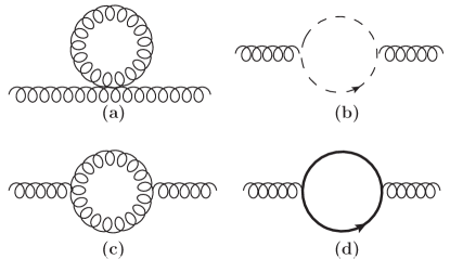
Figure 4: Diagrams contributing to the gluon (first two lines) and ghost (last line) self-energy at leading order in standard perturbation theory.

By inspection, we find that the set of diagrams with the same powers of $g_{g}^{2}$ and $1/N_{c}$ are obtained by dressing the quark propagator according to Fig. 3, as represented by the thick line in diagram (d) of Figure 4.

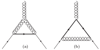
Figure 5: One-loop-order diagrams contributing to the quark-gluon vertex. The standard one-loop structures are identical, with the resummed (thick) quark line replaced by the tree-level one. Diagram (a) involves a three-gluon coupling whereas diagram (b) is $1/N_{c}$ supressed because all the gluon lines are not in the same side of the quark line. In fact, this diagram is of order $1/N_{c}^{2}$ and is thus subdominant in the RI-loop expansion.

Another interesting example is the quark-gluon vertex at RI-one-loop; see Fig. 5. Diagram (a) is of order $g_{g}$ and diagram (b) is naively suppressed by a factor $1/N_{c}$ respect to the tree-level contribution. In fact, the suppression is rather of order $1/N_{c}^{2}$ because the $1/N_{c}$ contribution involves a factor ${\rm tr}\,t^{a}=0$. It is, thus, subleading in the RI-loop expansion. As it was the case for the gluon self-energy, the complete set of diagrams of order $g_{g}$ is obtained by dressing the quark propagators according to Fig. 3. The set of diagrams of order $1/N_{c}^{2}$ is richer. Indeed, on top of dressing the quark propagators in the diagram (b) of Fig. 5, we can also add infinitely many gluon ladders between the two quark legs. It is interesting to note that these are all ultraviolet finite and, accordingly, do not contribute to the running of the quark-gluon coupling in the ultraviolet regime.

We finally discuss the case of the meson propagator. The diagrams contributing at RI-1-loop order are depicted in Fig. 6, where it is understood that the quark propagators are dressed according to the previous analysis; see, in particular, Eq. (6). The meson propagator includes the infinite set of ladder diagrams and the present approximation coincides at leading order with the rainbow-ladder approximation for the meson spectroscopy. This infinite series can be conveniently be written in terms of a dressed quark-antiquark-meson vertex, as represented in Fig. 6, which satisfies the linear integral equation depicted in Fig. 7. The latter clearly produces the required ladder diagrams when formally iterated in powers of the one-gluon-exchange rung. However, unlike this formal series, the integral equation for the meson vertex has a well-defined meaning and can be solved by standard (numerical) methods.

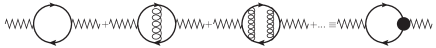
Figure 6: The infinite series of (ladder) diagrams contributing to the meson propagator at RI-one-loop order: each new rung brings additional factors $g_{q}^{2}/N_{c}$ from the vertices and $N_{c}$ from a color loop. The infinite sum can be cast in a dressed quark-antiquark-meson vertex.

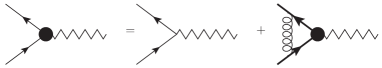
Figure 7: The linear integral equation for the quark-antiquark-meson vertex. The formally generates the infinite series of one-gluon-exchange ladder diagrams.

To summarize, the double expansion in $g_{g}$ and $1/N_{c}$ reproduces, at leading order, the standard rainbow-ladder approximation. Obtaining this very powerful approximation of QCD in the framework of a systematic expansion has three main assets. First, the justification of this approximation arises from a genuine analysis of the relative values of the couplings in QCD coming from lattice simulations. To the best of our knowledge, the fact that the rainbow-ladder approximation can be obtained from such a systematic expansion has not been formulated before. Second, the present analysis allows for a precise organization of subleading corrections to the rainbow-ladder whose contributions can, at least in principle, be computed. This precise organization of the expansion has important technical consequences. As we show below, it enables us to ontrol both the ultraviolet divergences and the RG improvement of the equations (in general, a nontrivial issue for nonperturbative approximations Fischer03 ) in a consistent way. Third, it motivates the structure of the gluon propagator that has to be used in actual calculations. In general, this requires some modeling on top of the rainbow-ladder approximation. Here, this comes directly from the success of the present model in the gluon/ghost sector. We emphasize, however, that the renormalization program beyond the leading-order approximation is subtle. In fact the asymmetrical treatment of the quark and ghost-gluon sectors may lead to the breaking of the massive version of the BRST symmetry, a symmetry that ensures the perturbative renormalizability of the theory (1). As a consequence, the renormalization program beyond leading order may require further work. This goes beyond the scope of the present article.

IV Implicit equations for the quark propagator

In this section, we analyse in detail the quark propagator at leading-order in the RI-loop expansion. The integral equation depicted in Eq. (6) reads

$$S^{-1}_{\Lambda}(p) =-i\not{p}+M_{\Lambda}$$

$$+g_{\Lambda}^{2}\int_{|q|<\Lambda}\gamma_{\mu}t^{a}S_{\Lambda}(q)\gamma_{\nu}t^{b}G_{0,\mu\nu}^{ab}(q+p),$$ (7)

where $S_{\Lambda}$ represents the (unrenormalized) quark propagator. Here, we have used an ultraviolet cutoff $\Lambda$ to regularize possible divergences in the loop integral.

As usual, finite correlation functions (that we note without the $\Lambda$ subscript) are obtained by introducing renormalized fields

$$A_{\mu,\Lambda}^{a}=\sqrt{Z_{A}}A_{\mu}^{a}\quad{\rm and}\quad\psi_{\Lambda}=\sqrt{Z_{\psi}}\psi,$$ (8)

and renormalized masses and coupling constant

$$m_{\Lambda}^{2}=Z_{m^{2}}m^{2},\quad M_{\Lambda}=Z_{M}M,\,\,\,{\rm and}\quad g_{q,\Lambda}=Z_{g_{q}}g_{q}.$$ (9)

The renormalization factors of the quark sector can be fixed by the prescription

$$S^{-1}(p=\mu_{0},\mu_{0})=-i\not{\mu}_{0}+M(\mu_{0}),$$ (10)

where, for short, we use the same notation $\mu_{0}$ for the RG scale and for an Euclidean vector of norm $\mu_{0}$. We consider first a strict version of the approximation and defer the detailed discussion of RG effects to a subsequent section.

Equation (IV) can be decomposed in a scalar and a vectorial component and expressed in terms of renormalized quantities. We get

$$Z_{\psi}^{-1}(\mu_{0})A(p,\mu_{0}) =1-Z_{g_{q}}^{2}(\mu_{0})g_{q}^{2}(\mu_{0})C_{F}\int_{|q|<\Lambda}Z_{\psi}(\mu_{0})\tilde{A}(q,\mu_{0})\frac{f(q,p)Z_{A}(\mu_{0})}{Z_{A}(\mu_{0})[(p+q)^{2}+Z_{m^{2}}(\mu_{0})m^{2}(\mu_{0})]},$$ (11)

$$Z_{\psi}^{-1}(\mu_{0})B(p,\mu_{0}) =Z_{M}(\mu_{0})M(\mu_{0})+Z_{g_{q}}^{2}(\mu_{0})g_{q}^{2}(\mu_{0})C_{F}\int_{|q|<\Lambda}Z_{\psi}(\mu_{0})\tilde{B}(q,\mu_{0})\frac{(d-1)Z_{A}(\mu_{0})}{Z_{A}(\mu_{0})[(p+q)^{2}+Z_{m^{2}}(\mu_{0})m^{2}(\mu_{0})]},$$ (12)

with

$$f(q,p)\equiv\frac{2p^{2}q^{2}+3(p^{2}+q^{2})(p\cdot q)+4(p\cdot q)^{2}}{p^{2}(q+p)^{2}}\,.$$ (13)

Our notation for $A$ and $B$ (and correspondingly for $\tilde{A}$ and $\tilde{B}$) makes explicit that these functions depend on $\mu_{0}$ through the renormalization scale used to define the renormalized coupling and masses. For later convenience, we have combined the renormalization factors with the associated renormalized quantities in such a way that they reconstruct the corresponding, $\mu_{0}$-independent, bare quantities. For instance $Z_{\psi}(\mu_{0})\tilde{A}(q,\mu_{0})=\tilde{A}_{\Lambda}(q)$ is independent of $\mu_{0}$. For $SU(N_{c})$, $C_{F}=(N_{c}^{2}-1)/(2N_{c})\sim N_{c}/2$. Accordingly, for large $N_{c}$, $g_{q}^{2}C_{F}\sim\lambda/2$ has a finite limit.

We now discuss the renormalization of Eqs. (11) and (12). For consistency, we must treat the renormalization factors in Eqs. (11) and (12) at the order of approximation considered here, i.e., at order $g_{g}^{0}$ and $1/N_{c}^{0}$. To this end, we recall that the first correction to the gluon self-energy and quark-gluon vertex are either of order $g_{g}$ or $1/N_{c}$ (see Sec. III). Consequently, $Z_{A}$, $Z_{m^{2}}$ and $\sqrt{Z_{A}}Z_{\psi}Z_{g_{q}}$ can all be set to 1 in Eqs. (11) and (12). Next, we observe that the integral in Eq. (11) is finite for functions $A(p)$ and $B(p)$ behaving as the bare expressions (up to logarithmic corrections). We can therefore consistently take $Z_{\psi}$ finite. Its precise value is fixed by the condition (10) as explained below. This generalizes the known result that, in the Landau gauge, the quark renormalization factor is finite at one-loop order in standard perturbation theory; see, e.g., Ref. Gracey:2002yt .

We are thus left with the following equations at leading order

$$A(p,\mu_{0}) =Z_{\psi}(\mu_{0})$$

$$-g_{q}^{2}(\mu_{0})C_{F}\int_{|q|<\Lambda}\tilde{A}(q,\mu_{0})\frac{f(q,p)}{(p+q)^{2}+m^{2}(\mu_{0})},$$ (14)

$$B(p,\mu_{0}) =Z_{\psi}(\mu_{0})Z_{M}(\mu_{0})M(\mu_{0})$$

$$+g_{q}^{2}(\mu_{0})C_{F}\int_{|q|<\Lambda}\tilde{B}(q,\mu_{0})\frac{d-1}{(p+q)^{2}+m^{2}(\mu_{0})}\,.$$ (15)

The ultraviolet divergence of the momentum integral in Eq. (IV) can be absorbed in the bare quark mass term (first term on the right-hand side) and the renormalized equation is, consequently, finite. It is actually more convenient to consider expressions with no divergence at all. To do so, we compute the difference between $B(p,\mu_{0})$ and $B(\mu_{0},\mu_{0})=M(\mu_{0})$ (note that $A(\mu_{0},\mu_{0})=1$), which yields

$$B(p,\mu_{0})=M(\mu_{0})+g_{q}^{2}(\mu_{0})C_{F}(d-1)\times$$ (16)

$$\int_{q}\tilde{B}(q,\mu_{0})\left(\frac{1}{(p+q)^{2}+m^{2}(\mu_{0})}-\frac{1}{(\mu_{0}+q)^{2}+m^{2}(\mu_{0})}\right)\,.$$ (17)

The integral is now finite and we can safely take the limit $\Lambda\to\infty$, if $\tilde{B}(q,\mu_{0})$ decreases fast enough as a function of $q$ in the ultraviolet. Note also that it does not have large logarithmic contributions as long as $p\sim\mu_{0}$ because the integrand is suppressed for $q\ll\mu_{0}$ or $q\gg\mu_{0}$ as compared to the region $q\sim\mu_{0}$.

V Renormalization-Group improvement

We could now try to find the self-consistent solutions of the previous equations which are just a particular realization of the rainbow approximation mentioned in the Introduction. However, this direct solution has the difficulty that the ultraviolet tails are not under control. Indeed, we observe that the integral in the right hand side of Eq. (17) involves large logarithms $\sim\ln(p/\mu_{0})$ which spoil the validity of perturbation theory. To make this point more explicit, let us study the ultraviolet behavior of the solutions of Eqs. (IV) and (17). In this regime, where asymptotic freedom holds, we should retrieve the results of standard perturbation theory, ie $A(p)\sim 1$ and $B(p)\sim(\ln p)^{\alpha}$ where $\alpha<0$ is given by an actual one-loop calculation. Instead, plugging these ultraviolet behaviors on the right-hand side of Eq. (17), we find that the integral behaves as $(\ln p)^{\alpha+1}$ when $p\gg m$, which is not consistent with the (assumed) behavior of the left-hand side. We get a clue of the origin of the problem by observing that we do retrieve the perturbative solution if we replace the coupling constant $g_{q}(\mu_{0})$ by a running coupling constant $g_{q}(p)$ in Eq. (17). The reason is now clear, for $p\gg\mu_{0}$, Eq. (17) is not under control: even if the expansion parameters $\alpha_{g}$ and $1/N_{c}$ are small, large logarithms spoil its validity in that regime. This is the standard problem of large logarithms in perturbation theory, which can be dealt with by means of the RG improvement.

To do so, we first make use of the RG equation:

$$(\mu\partial_{\mu}-\gamma_{\psi}+\beta_{X_{i}}\partial_{X_{i}})S^{-1}=0$$ (18)

where $X_{i}$ represents the various coupling constants and masses of the theory, $\beta_{X_{i}}=\mu\partial_{\mu}X_{i}$ are the associated beta functions, and

$$\gamma_{\psi}=\mu\partial_{\mu}\ln Z_{\psi}.$$ (19)

This equation states that the same correlation functions can be obtained if the normalization prescriptions are fixed at a different scale $\mu$,

$$S^{-1}(p=\mu,\mu)=-i\not{\mu}+M(\mu),$$ (20)

provided that the coupling constants and masses are solutions of the flow equations. This change of RG scale leads to a change of normalization of the correlation function that can be fixed by integrating the RG equation:

$$S^{-1}(p,\mu,X_{i}(\mu))=z_{\psi}(\mu,\mu_{0})S^{-1}(p,\mu_{0},X^{0}_{i}),$$ (21)

with $X_{i}^{0}=X_{i}(\mu_{0})$ and

$$\ln z_{\psi}(\mu,\mu_{0})=\int_{\mu_{0}}^{\mu}\frac{d\mu^{\prime}}{\mu^{\prime}}\gamma_{\psi}(\mu^{\prime}).$$ (22)

Evaluating now the previous equation at $\mu=p$ and using the normalization condition Eq. (20), we deduce that

$$A(p,\mu_{0}) =z_{\psi}^{-1}(p,\mu_{0}),$$ (23)

$$B(p,\mu_{0}) =z_{\psi}^{-1}(p,\mu_{0})M(p).$$ (24)

We are thus left with the question of determining $z_{\psi}(p,\mu_{0})$ and $M(p)$. To that aim, we need to change the renormalization scale while keeping the bare quantities fixed. Of course this will simultaneously imply the running of the parameters in the pure gauge sector (gluon mass and couplings). We shall first determine the functions $z_{\psi}(p,\mu_{0})$ and $M(p)$ and then discuss the running of the remaining parameters.

V.1 Running of $M(p)$ and expression for $z_{\psi}$

From the renormalization condition (20) applied to Eq. (12) with $\mu_{0}=p$, we obtain the relation

$$\begin{split}&Z^{-1}_{\psi}(p)M(p)=Z_{M}(p)M(p)+Z_{g_{q}}^{2}(p)g_{q}^{2}(p)C_{F}(d-1)\\ &\times\int_{|q|<\Lambda}Z_{\psi}(p)\tilde{B}(q,p)\frac{1}{(q+p)^{2}+Z_{m^{2}}(p)m^{2}(p)}\,.\end{split}$$ (25)

We now take a $p$-derivative at fixed bare quantities and obtain

$$\begin{split}&pM^{\prime}(p)-\gamma_{\psi}(p)M(p)=-Z_{\psi}^{2}(p)Z^{2}_{g_{q}}(p)g^{2}_{q}(p)C_{F}(d-1)\\ &\times\int_{|q|<\Lambda}\tilde{B}(q,p)\frac{2p^{2}+2p.q}{[(q+p)^{2}+Z_{m^{2}}(p)m^{2}(p)]^{2}}\,.\\ \end{split}$$ (26)

Observe that the integral in the previous equation is ultraviolet finite and we can send the cutoff $\Lambda$ to infinity. We finally replace $A$ and $B$ according to Eqs. (23) and (24) and keep only the terms of order $g_{g}^{0}$ and $N_{c}^{0}$ (i.e., $Z_{m^{2}}=Z_{\psi}Z_{g_{q}}=1$). We then arrive at the equation

$$\begin{split}&pM^{\prime}(p)=\gamma_{\psi}(p)M(p)-g^{2}_{q}(p)C_{F}(d-1)\\ &\times\int_{q}z_{\psi}(q,p)\frac{M(q)}{q^{2}+M^{2}(q)}\frac{2p^{2}+2p.q}{\left[(q+p)^{2}+m^{2}(p)\right]^{2}}\,.\\ \end{split}$$ (27)

We now derive a similar equation for $z_{\psi}$. The renormalization condition (20) applied to Eq. (11) with $\mu_{0}=p$ leads to

$$Z^{-1}_{\psi}(p) =1-Z^{2}_{g_{q}}(q)g_{q}^{2}(p)C_{F}$$

$$\times\int_{q}Z_{\psi}(p)\tilde{A}(q,p)\frac{f(q,p)}{(p+q)^{2}+Z_{m^{2}}(p)m^{2}(p)}\,.$$ (28)

The anomalous dimension, which is needed in Eq. (27), is obtained by taking a $p$-derivative at fixed bare theory. We obtain

$$\begin{split}\gamma_{\psi}(p)=g_{q}^{2}(p)C_{F}\int_{q}&\frac{z_{\psi}(q,p)}{q^{2}+M^{2}(q)}\Bigg{[}\frac{p_{\mu}\frac{\partial}{\partial{p_{\mu}}}f(q,p)}{(p+q)^{2}+m^{2}(p)}\\ &-\frac{2(p^{2}+p.q)f(q,p)}{((p+q)^{2}+m^{2}(p))^{2}}\Bigg{]},\end{split}$$ (29)

where, again, we have kept only terms of order $g_{g}^{0}$ and $N_{c}^{0}$ and we have used Eqs. (23) and (24). We note that a benefit of the present (semi)perturbative treatment is that the running coupling constant appears naturally in the flow equations (27) and (29). This plays a crucial role in obtaining the correct S$\chi$SB solutions Miransky:1984ef ; Atkinson:1988mw , which usually requires an appropriate modeling of the quark-gluon vertex in nonperturbative setups Fischer03 .

We observe that Eqs. (26) and (29) still involve $z_{\psi}$ and we have to relate this quatity to $M$ and $Z_{\psi}$ to obtain a closed system of equations. Because $Z_{\psi}$ is finite, we trivially obtain, from Eq. (19),

$$z_{\psi}(p,\mu_{0})=Z_{\psi}(p)/Z_{\psi}(\mu_{0}),$$ (30)

with

$$Z_{\psi}(p)=1+g_{q}^{2}(p)C_{F}\int_{q}\frac{z_{\psi}(q,p)}{q^{2}+M^{2}(q)}\frac{f(q,p)}{(p+q)^{2}+m^{2}(p)}\,,$$

which is obtained from Eq. (V.1) using $Z_{g_{q}}(p)Z_{\psi}(p)=1$ and solving for $Z_{\psi}(p)$. As a consequence, only functions of a single variable [$M(p)$ and $Z_{\psi}(p)$] have to be considered. We mention that we have a priori two different formulae for $z_{\psi}$, either Eq. (30) or Eq. (23). The way they are related is discussed in Appendix A.

V.2 Running of the coupling constant and of the gluon mass

The set of equations (26) and (29) is not closed yet because there appear the gluon mass and the quark-gluon coupling at a running scale. In our approximation, this can be deduced from a calculation of the quark-gluon vertex and the gluon propagator at the same level of approximation. This can be performed by following the procedure described before. However for the purposes of the present paper, we will consider a simplified approximation where the runnings of the coupling and the mass are given by simple but realistic ansätze. We defer a more systematic analysis in the present approximation scheme to a future work.

On the one hand, the gluon mass decreases logarithmically at large $\mu$ Tissier:2011ey . This slow evolution is expected to have little influence on the integrals appearing in the implicit equations (26) and (29). In the following, we just neglect this effect and replace $m(\mu)$ by some scale-independent value $m(\mu_{0})=m_{0}$.

On the other hand, asymptotic freedom implies that the quark-gluon coupling $g_{q}(\mu)$ tends to zero in the deep ultraviolet (where all couplings have a universal running). Consequently, in this regime, the resummed diagrams depicted in Fig 5 simplifies greatly and we are left with the usual one-loop expression for the beta function

$$\beta_{g}=-\beta_{0}g^{3}(\mu),$$ (32)

with

$$\beta_{0}=\frac{1}{16\pi^{2}}\Big{(}\frac{11}{3}N_{c}-\frac{2}{3}N_{f}\Big{)},$$ (33)

where $N_{f}$ is the number of light quarks. Equation (32) is solved as

$$g^{2}(\mu)=\frac{g^{2}(\mu_{0})}{1+\beta_{0}g^{2}(\mu_{0})\ln(\mu^{2}/\mu_{0}^{2})}.$$ (34)

This behavior is valid as long as the RG scale is much larger than the (quark and gluon) masses. However, there is an intermediate regime where $\mu\gg m_{0}$ but where the quark-gluon coupling is still too large to apply the usual perturbation theory. This intermediate regime could be studied by calculating the full beta function in the RI-1-loop order, as explained above; see Fig 5. Instead, in this work, we use the perturbative running and include by hand a smooth freeze-out when $\mu\simeq m_{0}$. Again, a more systematic treatment is deferred to a future work. In practice, we employ the following expression for the quark-gluon running

$$g_{q}^{2}(\mu)=\frac{g^{2}_{0}}{1+\beta_{0}g_{0}^{2}\ln\Big{(}\frac{\mu^{2}+x^{2}m_{0}^{2}}{x^{2}m_{0}^{2}}\Big{)}}$$ (35)

where $x$ is a free parameter that fixes the precise point of freeze-out. An asset of this simple truncation is that we can vary the size of the quark-gluon vertex in the infrared and check that S$\chi$SB occurs only for large enough coupling $g_{0}$. However, we must stress that this is an artefact of our modelization (35). We mention also that our model for the running of the coupling is such that $g_{q}(\mu)$ increases with decreasing $\mu$ and saturates at $g_{0}$ as $\mu\to 0$. This behavior is not the one seen for instance in fRG flows Braun:2014ata where, the quark-gluon coupling after some dramatic increase, decreases as $\mu\to 0$. If the decrease takes place significantly below the constituent quark mass, this effect should not have an important effect in the present analysis. Would we treat systematically the ladder diagrams of the quark-gluon vertex, the infrared value of the quark-gluon vertex would not be a free parameter anymore and the variation of $g_{q}$ would be more realistic. This is under current investigation. In principle, one should do the same procedure for the gluon anomalous dimensions also, but again, we neglect this effect in the present article.

VI Implementation and results

We now detail our numerical procedure to solve the coupled equations (26) and (29), together with the evolution of the coupling constant (35). We first perform the angular integrals and obtain expressions where only a one-dimensional integral needs to be performed numerically. We then discuss the behavior of the functions $M(p)$ and $Z_{\psi}(p)$ when $p\gg m$. This information is important for controlling numerically the ultraviolet tails of the integrals. We then describe the numerical resolution of the problem and present our results.

VI.1 Angular integration

To simplify the study of Eqs. (26) and (29), we first perform analytically all angular integrals except the one over the angle $\theta$ between the vectors $p$ and $q$. Defining $u=\cos\theta$ we obtain

$$\begin{split}Z_{\psi}(p)=1+\frac{g_{q}^{2}(p)C_{F}\Omega_{d-1}}{p^{2}Z_{\psi}(p)(2\pi)^{d}}\int_{0}^{\infty}dq&\hskip 2.84526ptq^{d-1}\frac{Z_{\psi}(q)}{q^{2}+M^{2}(q)}\times\\ &\int_{-1}^{1}du(1-u^{2})^{\frac{d-3}{2}}\frac{2p^{2}q^{2}+3(p^{2}+q^{2})pqu+4p^{2}u^{2}q^{2}}{\left(p^{2}+2pqu+q^{2}\right)\left(p^{2}+2pqu+q^{2}+m_{0}^{2}\right)}\,,\end{split}$$ (36)

$$\begin{split}-\gamma_{\psi}(p)M(p)+pM^{\prime}(p)=-(d-1)\frac{g_{q}^{2}(p)C_{F}\Omega_{d-1}}{Z_{\psi}(p)(2\pi)^{d}}\int_{0}^{\infty}dq\ &\hskip 2.84526ptq^{d-1}\frac{Z_{\psi}(q)M(q)}{q^{2}+M^{2}(q)}\times\\ &\int_{-1}^{1}du(1-u^{2})^{\frac{d-3}{2}}\frac{2p^{2}+2puq}{(p^{2}+2qup+q^{2}+m_{0}^{2})^{2}}\,,\end{split}$$ (37)

where $\Omega_{d}=2\pi^{d/2}/\Gamma(d/2)$. In integer dimensions, and in particular in $d=4$ on which we concentrate from now on, the integral over $u$ can be done analytically, which yields

$$\begin{split}Z_{\psi}(p)=1+\frac{g_{q}^{2}(p)C_{F}}{32\pi^{2}p^{4}m_{0}^{2}Z_{\psi}(p)}&\int_{0}^{\infty}dq\,q\,\frac{Z_{\psi}(q)}{q^{2}+M^{2}(q)}\Big{\{}\left|p^{2}-q^{2}\right|^{3}-m_{0}^{4}\left[2m_{0}^{2}+3\left(p^{2}+q^{2}\right)\right]\\ &+\sqrt{2q^{2}\left(m_{0}^{2}-p^{2}\right)+\left(m_{0}^{2}+p^{2}\right)^{2}+q^{4}}\left[2m_{0}^{4}+m_{0}^{2}\left(p^{2}+q^{2}\right)-\left(p^{2}-q^{2}\right)^{2}\right]\Big{\}}\,,\end{split}$$ (38)

$$\begin{split}&-\gamma_{\psi}(p)M(p)+pM^{\prime}(p)=-\frac{3g_{q}^{2}(p)C_{F}}{8\pi^{2}p^{2}Z_{\psi}(p)}\int_{0}^{\infty}dq\,q\,\frac{Z_{\psi}(q)M(q)}{q^{2}+M^{2}(q)}\Bigg{[}m_{0}^{2}+q^{2}-\frac{m_{0}^{4}+m_{0}^{2}\left(p^{2}+2q^{2}\right)-p^{2}q^{2}+q^{4}}{\sqrt{m_{0}^{4}+2m_{0}^{2}\left(p^{2}+q^{2}\right)+\left(p^{2}-q^{2}\right)^{2}}}\Bigg{]}\,.\end{split}$$ (39)

There remains to compute the angular integrals for the anomalous dimension $\gamma_{\psi}$ given in Eq. (29). This calculation is very similar to the one performed here for $Z_{\psi}$. Formally, $\gamma_{\psi}$ is obtained by deriving Eq. (38) with respect to $p$ keeping the ratio $g_{q}^{2}(p)/Z_{\psi}(p)$ fixed on the right-hand side.

VI.2 The ultraviolet behaviour of the equations

Our strategy is now to look for self-consistent solutions to Eqs. (38) and (39), together with Eq. (35). In order to do so, we shall assume specific behaviors for the functions $Z_{\psi}(p)$ and $M(p)$ when $p\gg m_{0}$ and check for their self-consistency. In the next section, we shall verify explicitly the conclusions of such an analysis by numerically solving the full system of equations.

VI.2.1 Ultraviolet limit for $Z_{\psi}(p)$

We assume that $Z_{\psi}(p)$ behaves as some power of $\ln p$ in the ultraviolet limit ($p\gg m_{0}$). We also assume that $M(p)\ll p$ in that limit. By substituting these behaviors in Eq. (38), it is relatively straightforward to see that the loop term is suppressed by a positive power of $m_{0}^{2}/p^{2}$. Accordingly $Z_{\psi}(p)\to 1$ in that limit.

VI.2.2 Ultraviolet limit for $M(p)$

In the limit $p\gg m_{0}$, we find two solutions for the running mass $M(p)$. The first one, that we call “massive behavior”, decreases as an inverse power of $\ln p$. This is the expected behavior away from the chiral limit. As we show below, this solution is described by perturbation theory in the ultraviolet limit. When the bare mass is reduced and the chiral limit is approached, another solution appears (at least for sufficiently large coupling constant, see below), where $M(p)$ decreases as an inverse power law in $p$. This corresponds to the S$\chi$SB solution.

We first consider the massive case. We use that $Z_{\psi}(p)\to 1$ in the ultraviolet and study the self-consistency of solutions which behave as $M(p)\sim\ln^{\alpha}(p/m_{0})$ at large $p$. Given that $\gamma_{\psi}(p)$ goes to zero as a power law in $p$, the term including $\gamma_{\psi}(p)$ can always be neglected with respect to $pM^{\prime}(p)$. Consider then the integral in the right-hand side of Eq. (39) and divide it in three parts: $q\gg p$, $m_{0}\ll q\lesssim p$, and $q\lesssim m_{0}$. The behaviors of the integral in these three regions (together with the logarithmic running of $g_{q}$) are summarized in Table 1.

$pM^{\prime}(p)$	$q\gg p$	$m_{0}\ll q\lesssim p$	$q\sim m_{0}$
$\ln^{\alpha-1}p$	$p^{-2}\ln^{\alpha-1}p$	$\ln^{\alpha-1}p$	$p^{-2}\ln^{-1}p$

Table 1: Large-$p$ behavior of Eq. (39) for the massive solution. The first column is the assumed UV behavior of the left-hand side of the equation whereas the last three columns are the contributions from the different regions of integration on the right-hand side [including the prefactor $g_{q}^{2}(p)/p^{2}$].

From this analysis, we conclude that, a priori, there are self-consistent solutions for any value of $\alpha$ in the massive case. We can also observe that, in the massive solution, the integral in Eq. (39) is dominated by momenta of the order $q\sim p\gg m_{0}$. This enables us to make contact with perturbation theory. Indeed, in this regime, we can substitute the perturbative approximation $M(q)=M_{0}\ln^{\alpha}(q/m_{0})$ in the integrals. This allows us to approximate

$$\frac{M(q)}{q^{2}+M^{2}(q)}\sim\frac{M_{0}\ln^{\alpha}(q/m_{0})}{q^{2}}$$ (40)

and the bracket in Eq. (39) simplifies to $2q^{2}\Theta(p^{2}-q^{2})$. The integral can now be computed easily and we get

$$\alpha M_{0}\ln^{\alpha-1}(p/m_{0})=-g^{2}(p)\tilde{\gamma}_{M}M_{0}\ln^{\alpha}(p/m_{0})$$ (41)

where $\tilde{\gamma}_{M}=3C_{F}/(8\pi^{2})$. By using the ultraviolet running of the coupling constant Eq. (34), we conclude that

$$\alpha=-\frac{\tilde{\gamma}_{M}}{2\beta_{0}}.$$ (42)

One obtains the same result as with the standard perturbative analysis. Indeed, the latter gives

$$\beta_{M}=\mu\frac{dM}{d\mu}=-M\gamma_{M}=-\tilde{\gamma}_{M}Mg^{2}(\mu)+\mathcal{O}(g^{4}),$$ (43)

whose solution is, using the perturbative running of the coupling (34),

$$\frac{M}{M_{0}}=\left[1+2\beta_{0}g_{0}^{2}\ln\left(\frac{\mu}{\mu_{0}}\right)\right]^{-\frac{\tilde{\gamma}_{M}}{2\beta_{0}}},$$ (44)

in agreement with the direct analysis of Eq. (39).

Next, we want to find the ultraviolet limit of the S$\chi$SB solution. We assume that $M(p)\sim p^{\omega}\ln^{\delta}(p/m_{0})$ and repeat the same analysis as in the massive case. We restrict the analysis to $\omega<1$ to ensure that $M(q)\ll q$ when $q\gg m$. Here, one has to treat the cases $\omega$ larger, smaller or equal to $-2$ separately. In the last case, we need also to distinguish the cases $\delta$ larger, smaller or equal to $-1$. These various cases are summarized in Table 2 and we see that the only consistent solution of this type corresponds to $\{\omega=-2,\delta>-1\}$, where the dominant contribution comes from the regime $m_{0}\ll q\lesssim p$ as expected Atkinson:1988mw ; Miransky:1986ib .

$pM^{\prime}(p)$	$q\gg p$	$m_{0}\ll q\lesssim p$	$q\sim m_{0}$
$p^{\omega>-2}\ln^{\delta}p$	$m^{2}_{0}p^{\omega-2}\ln^{\delta-1}p$	$p^{\omega}\ln^{\delta-1}p$	$p^{-2}\ln^{-1}p$
$p^{\omega<-2}\ln^{\delta}p$	$m^{2}_{0}p^{\omega-2}\ln^{\delta-1}p$	$p^{-2}\ln^{-1}p$	$p^{-2}\ln^{-1}p$
$p^{-2}\ln^{\delta>-1}p$	$m^{2}_{0}p^{-4}\ln^{\delta-1}p$	$p^{-2}\ln^{\delta}p$	$p^{-2}\ln^{-1}p$
$p^{-2}\ln^{\delta<-1}p$	$m^{2}_{0}p^{-4}\ln^{\delta-1}p$	$p^{-2}\ln^{-1}p$	$p^{-2}\ln^{-1}p$
$p^{-2}\ln^{-1}p$	$m^{2}_{0}p^{-4}\ln^{-2}p$	$p^{-2}\ln(\ln p)\ln^{-1}p$	$p^{-2}\ln^{-1}p$

Table 2: Large-$p$ behavior of Eq. (39) for the S$\chi$SB solution. The first column is the assumed UV behavior of the left-hand side of the equation whereas the last three columns are the contributions from the different regions of integration on the right-hand side [including the prefactor $g_{q}^{2}(p)/p^{2}$]. We have distinguished the cases $\omega>-2$, $\omega<-2$, $\{\omega=-2,\delta>-1\}$, $\{\omega=-2,\delta<-1\}$ and $\{\omega=-2,\delta=-1\}$. Only the third case yields a possible consistent solution.

To compute the exponent $\delta$, we can thus safely set $m_{0}=0$ in the integrand of Eq. (39). As before, the term in brackets becomes $2q^{2}\Theta(p^{2}-q^{2})$ and, further using $Z_{\psi}(p)\to{\rm const}$ and neglecting $M^{2}(q)\ll q^{2}$ in the denominator of the integrand, we arrive at

$$pM^{\prime}(p)\approx-\frac{3g_{q}^{2}(p)C_{F}}{8\pi^{2}p^{2}}\int_{m_{0}^{2}}^{p^{2}}dq^{2}\,M(q)\,.$$ (45)

Plugging $M(p)\propto p^{-2}\ln^{\delta}p$ and extracting the multiplicative constant of the leading contribution for large $p$, we find that a consistent solution requires

$$1+\delta=-\alpha=\frac{9C_{F}}{11N_{c}-2N_{f}},$$ (46)

which reproduces the known results in the rainbow-ladder approximation Atkinson:1988mw ; Miransky:1986ib ; Fischer03 ; Aguilar:2010cn . We stress that the proper implementation of the running the coupling is a key ingredient to obtain this result. The present perturbative RG treatment allows for a consistent implementation of the latter.

VI.3 Numerical implementation

In practice, for numerical purposes, the integral over $q$ is divided in two regions, one for $q<\Lambda_{1}=10\,{\rm GeV}$ and the ultraviolet region for $\Lambda_{1}<q<\Lambda_{2}=20\,{\rm GeV}$. In the second region the values of $Z_{\psi}(q)$ and $M(q)$ are replaced by their ultraviolet expressions, i.e.,

$$Z_{\psi}^{\text{UV}}(q) =1$$ (47)

$$M^{\text{UV}}(q) =b_{0}\left(\ln\frac{q^{2}+m_{0}^{2}}{m_{0}^{2}}\right)^{\alpha}+\frac{b_{2}}{q^{2}}\left(\ln\frac{q^{2}+m_{0}^{2}}{m_{0}^{2}}\right)^{-(\alpha+1)}$$ (48)

where the exponent $\alpha$ is given in Eq. (42). The coefficients $b_{0}$ and $b_{2}$ are chosen in order to make $M(p)$ continuous and differentiable (so they are not free parameters).

For $p<\Lambda_{1}$, we sample the functions $Z_{\psi}(p)$ and $M(p)$ on a regular grid with a lattice spacing of $0.05\,{\rm GeV}$. We have verified that the results presented below are converged with respect to this choice. We solve the self-consistent equations for the functions $Z_{\psi}(p)$ and $M(p)$ iteratively with initial conditions provided by their respective perturbative expressions (48) and (48), with a fixed value of $M(\Lambda_{1})$.

VI.4 Chiral and massive behaviours

In Fig. 8, solutions for Eqs. (38) and (39) are shown for different values of $M(\Lambda_{1})$ for $g_{0}=4$ and $x=5$. No chiral solution is found for this small value of $g_{0}$. However for $g_{0}=11$ a chiral solution appears as shown in Fig. 9.

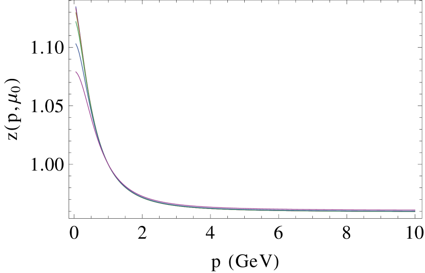
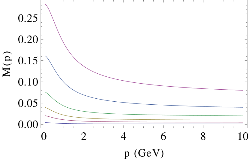
Figure 8: Solutions of Eqs. (38) and (39), $Z_{\psi}(p)$ and $M(p)$ for different values of $M(\Lambda_{1})=0.001,0.005,0.01,0.02,0.04,0.08$. Parameters: $N_{f}=2$, $N_{c}=3$, $m_{0}=0.4$ GeV, $g_{0}=4$ and $x=5$.

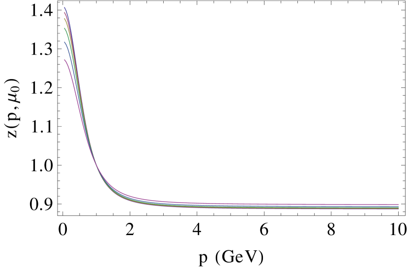
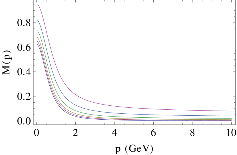
Figure 9: Solutions of Eqs. (38) and (39), $Z_{\psi}(p)$ and $M(p)$ for different values of $M(\Lambda_{1})=0.001,0.005,0.01,0.02,0.04,0.08$. Parameters: $N_{f}=2$, $N_{c}=3$, $m_{0}=0.4$ GeV, $g_{0}=11$ and $x=5$.

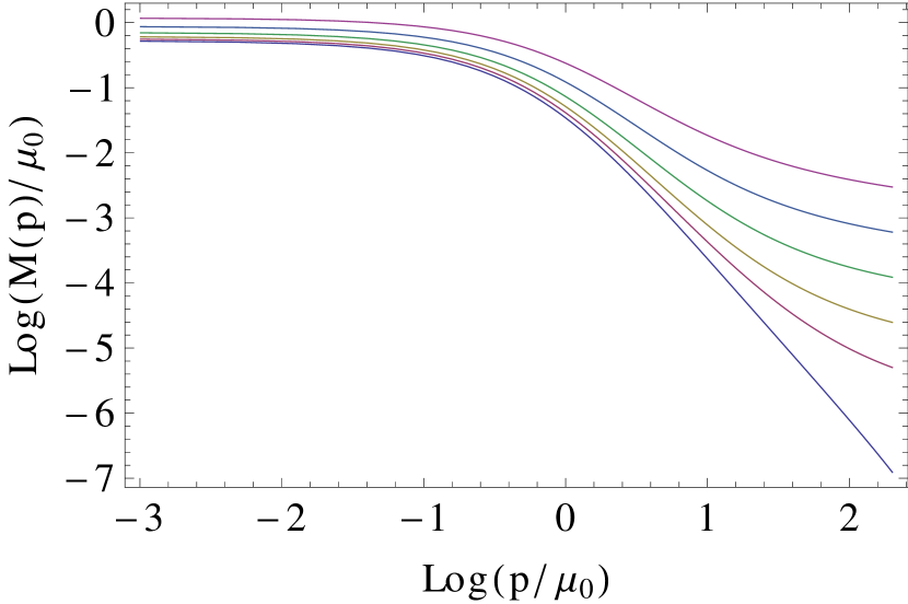
Figure 10: Mass function $M(p)$ in Log-Log scale for different values of $M(\Lambda_{1})=0.001,0.005,0.01,0.02,0.04,0.08$. Parameters: $N_{f}=2$, $N_{c}=3$, $m_{0}=0.4$ GeV, $g_{0}=11$ and $x=5$. We observe the onset of the power law behavior at large momentum as the chiral limit is approached. This signals the S$\chi$SB.

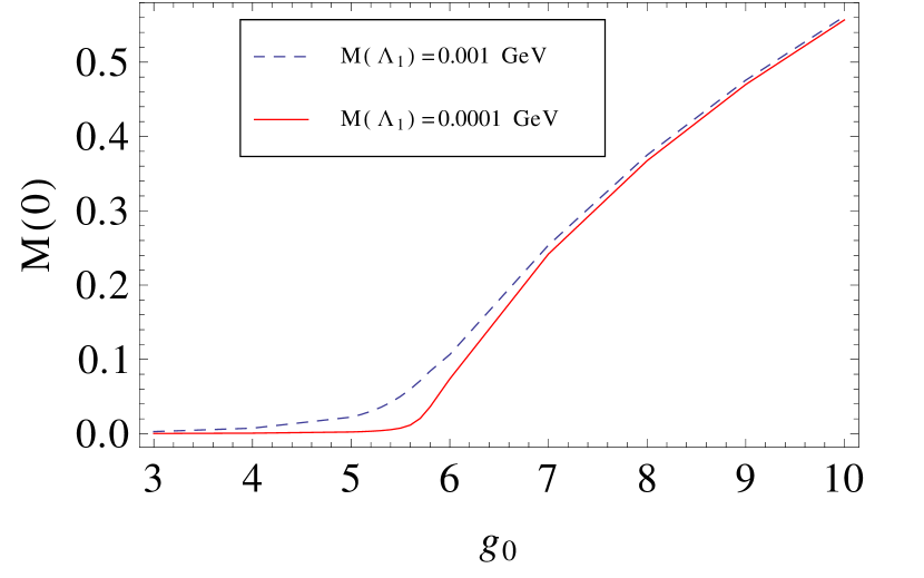
Figure 11: Constituent quark mass $M(p=0)$ as a function of the coupling parameter $g_{0}$ for two values of the ultraviolet mass $M(\Lambda_{1})$. The variation of $g_{0}$ is done by keeping $\Lambda_{QCD}$ fixed.

Unfortunately, in both cases the behaviour of $A(p,\mu_{0})=z^{-1}_{\psi}(p,\mu_{0})=Z_{\psi}(\mu_{0})/Z_{\psi}(p)$ is not the correct one. This is the same problem as with the one-loop results of Ref. Pelaez:2014mxa . There, it was also observed that the inclusion of two-loop corrections gave the correct shape of this function as explained in the Introduction. We expect this fuction to be better described at RI-2-loop order. In Fig. 10 the mass curve $M(p)$ is represented in a Log-Log scale. One can observe the approach in the chiral limit to an (approximate) power-law behavior.

Finally in Fig. 11, we illustrate the two—chirally symmetric versus chirally broken—phases of the system by plotting the constituent quark mass $M(p=0)$ as a function of the coupling parameter $g_{0}$ (when varying $g_{0}$ we vary also $x$ in such a way to keep $\Lambda_{QCD}$ fixed). This is done for two values of the ultraviolet mass $M(\Lambda_{1})$ very close to the chiral limit. Observe that, as expected, the convergence to the chiral limit is very slow for couplings approaching the critical value.

VI.5 Comparison with lattice data for $N_{f}=2$

Fig. 12 shows the comparison of the present results with lattice data from Ref. Oliveira:2016muq . This is done by fitting the parameters ($g_{0}$, $x$) so as to minimize the absolute error with all data-set simultaneously. After fixing those parameters, the various curves are fitted by varying the parameter $M(\Lambda_{1})$.

The agreement is quite stricking for the running mass $M(p)$. This is a qualitative improvement with respect to the one-loop results of Ref. Pelaez:2014mxa . This, of course, is due to the rainbow-improvement of the one-loop expressions in the quark sector. It is, indeed, well-known that the rainbow resummation gives good agreement with lattice data even near the chiral limit (see, for example, Refs. Roberts:2007jh ; Aguilar:2014lha ). As explained before, the main improvement of the present work is that this resummation proceeds from a systematic expansion scheme, which allows for a consistent RG improvement of the equations.

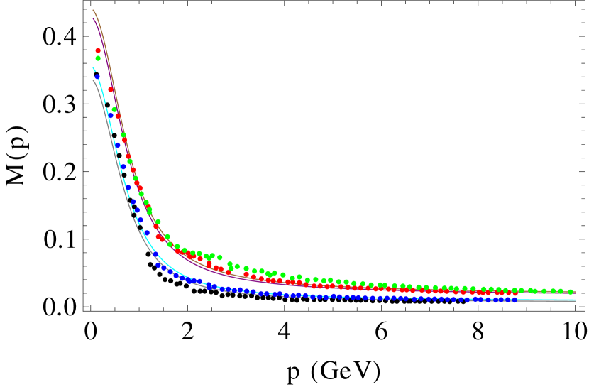
Figure 12: Comparision with lattice data from Oliveira:2016muq for $M(p)$ for $M(\Lambda_{1})=0.008,0.01,0.02,0.022$. Parametres: $N_{f}=2$, $N_{c}=3$, $m_{0}=0.4$ GeV, $g_{0}=7$ and $x=5$.

VII Conclusions

We have devised a systematic expansion scheme for QCD at low energy based on a double expansion in powers of the coupling strength $g_{g}$ in the Yang-Mills sector of the theory and in powers of $1/N_{c}$. It is based on the observation that, at low energies, the coupling $g_{g}$ differs significantly from the coupling $g_{q}$ in the quark sector. The motivation for the $1/N_{c}$ expansion is more practical and allows to obtain closed expression for the various correlation functions (let us point out however that the validity of the $1/N_{c}$ expansion in QCD is well established in the literature, see for instance Witten:1979kh ). At leading order, this scheme reproduces the well-known rainbow approximation. One of the benefits of our approach is however that it allows for a systematic study of higher order corrections. Moreover, at the present leading order, we are able to implement a consistent renormalization group improvement of the rainbow equations that yields a better control of large logarithms.

In the present work, we have considered a simplified running for the coupling. Among the possible extensions of the present work, it will be interesting to implement a realistic renormalization group equation for the quark-gluon coupling, based on the present approximation scheme. Another interesting extension is the analysis of the next approximation order in view of improving the description of the vectorial part of the quark propagator.

The present results open the way to applications mainly in two directions. First, we would like to use the present scheme to calculate mesonic properties such as the mass spectrum or decay rates. Given the well established success of the rainbow-ladder approximation Roberts:2007jh , this path seems promising. Second, we would like to explore the QCD phase diagram both at finite temperature and at finite chemical potential. The massive extension of QCD has been already applied with success for that purpose in the heavy-quark regime Reinosa:2015oua . The present work opens the way for the application of this model to the lower quark masses, including the chiral limit as well as physically realistic values.

Appendix A Compatibility of the formulae for $z_{\psi}$

In the core of the text, we found two different formulas for $z_{\psi}$. In this appendix, we discuss the compatibility of these expressions. The first expression

$$z_{\psi}^{-1}(p,\mu_{0})=\frac{1+g_{q}^{2}(\mu_{0})C_{F}\int_{q}\frac{z_{\psi}(q,\mu_{0})}{q^{2}+M^{2}(q)}\frac{f(q,\mu_{0})}{(\mu_{0}+q)^{2}+m^{2}(\mu_{0})}}{1+g_{q}^{2}(p)C_{F}\int_{q}\frac{z_{\psi}(q,p)}{q^{2}+M^{2}(q)}\frac{f(q,p)}{(p+q)^{2}+m^{2}(p)}}$$ (49)

is obtained by replacing in Eq. (30) the form of $Z_{\psi}$ given in Eq. (V.1). The second expression, obtained by combining Eqs. (23) and (IV), gives

$$z_{\psi}^{-1}(p,\mu_{0}) =Z_{\psi}(\mu_{0})$$

$$-g_{q}^{2}(\mu_{0})C_{F}\int_{q}\frac{z_{\psi}(q,\mu_{0})}{q^{2}+M^{2}(q)}\frac{f(q,p)}{(p+q)^{2}+m^{2}(\mu_{0})}$$ (50)

Using the fact that, to the order at which we are computing, $Z_{m^{2}}=Z_{\psi}Z_{g}=1$, we can write

$$z_{\psi}^{-1}(p,\mu_{0}) = Z_{\psi}(\mu_{0})\left\{1-Z_{g_{q}}^{2}(\mu_{0})g_{q}^{2}(\mu_{0})C_{F}\int_{q}Z_{\psi}(\mu_{0})\frac{z_{\psi}(q,\mu_{0})}{q^{2}+M^{2}(q)}\frac{f(q,p)}{(p+q)^{2}+Z_{m^{2}}(\mu_{0})m^{2}(\mu_{0})}\right\}$$ (51)

$$= Z_{\psi}(\mu_{0})\left\{1-Z_{g_{q}}^{2}(p)g_{q}^{2}(p)C_{F}\int_{q}Z_{\psi}(p)\frac{z_{\psi}(q,p)}{q^{2}+M^{2}(q)}\frac{f(q,p)}{(p+q)^{2}+m^{2}(\mu_{0})}\right\}$$

$$= Z_{\psi}(\mu_{0})\left\{1-\frac{g_{q}^{2}(p)}{Z_{\psi}(p)}C_{F}\int_{q}Z_{\psi}(p)\frac{z_{\psi}(q,p)}{q^{2}+M^{2}(q)}\frac{f(q,p)}{(p+q)^{2}+m^{2}(\mu_{0})}\right\}$$

which, owing to Eq. (V.1), is nothing but Eq. (49). We have used that $z_{\psi}(\mu_{0})Z_{\psi}(q,\mu_{0})$, $Z_{g_{q}}(\mu_{0})g_{q}(\mu_{0})$ and $Z_{m^{2}}(\mu_{0})m^{2}(\mu_{0})$ do not depend on $\mu_{0}$.

References

- (1) P. O. Bowman, U. M. Heller, D. B. Leinweber, M. B. Parappilly, A. G. Williams and J. b. Zhang, Phys. Rev. D 71, 054507 (2005).
- (2) O. Oliveira, A. Kizilersü, P. J. Silva, J. I. Skullerud, A. Sternbeck and A. G. Williams, arXiv:1605.09632.
- (3) W. Schleifenbaum, M. Leder and H. Reinhardt, Phys. Rev. D 73, 125019 (2006).
- (4) M. Quandt, H. Reinhardt and J. Heffner, Phys. Rev. D 89 065037 (2014).
- (5) L. von Smekal, R. Alkofer and A. Hauck, Phys. Rev. Lett. 79 (1997) 3591.
- (6) R. Alkofer and L. von Smekal, Phys.Rept.353 (2001) 281.
- (7) D. Zwanziger, Phys. Rev. D 65 (2002) 094039.
- (8) C. S. Fischer and R. Alkofer, Phys. Rev. D 67 (2003) 094020.
- (9) J. C. R. Bloch, Few Body Syst. 33 (2003) 111.
- (10) J. M. Pawlowski, D. F. Litim, S. Nedelko and L. von Smekal, Phys. Rev. Lett. 93, 152002 (2004).
- (11) C. S. Fischer and H. Gies, JHEP 0410, 048 (2004).
- (12) A. C. Aguilar and A. A. Natale, JHEP 0408 (2004) 057.
- (13) Ph. Boucaud et al., JHEP 06 (2006) 001.
- (14) A. C. Aguilar and J. Papavassiliou, Eur. Phys. J. A 35 (2008) 189.
- (15) A. C. Aguilar, D. Binosi and J. Papavassiliou, Phys. Rev. D 78 (2008) 025010.
- (16) P. Boucaud, J. P. Leroy, A. Le Yaouanc, J. Micheli, O. Pene and J. Rodriguez-Quintero, JHEP 06 (2008) 099.
- (17) C. S. Fischer, A. Maas and J. M. Pawlowski, Annals Phys. 324 (2009) 2408.
- (18) J. Rodriguez-Quintero, JHEP 1101 (2011) 105.
- (19) M. Q. Huber and L. von Smekal, JHEP 04, 149 (2013).
- (20) A. Sternbeck, L. von Smekal, D. B. Leinweber and A. G. Williams, PoS LAT 2007, 340 (2007).
- (21) A. Cucchieri and T. Mendes, Phys. Rev. Lett. 100, 241601 (2008).
- (22) A. Cucchieri and T. Mendes, Phys. Rev. D 78, 094503 (2008).
- (23) A. Sternbeck and L. von Smekal, Eur. Phys. J. C 68, 487 (2010).
- (24) A. Cucchieri and T. Mendes, Phys. Rev. D 81, 016005 (2010).
- (25) I. L. Bogolubsky, E. M. Ilgenfritz, M. Muller-Preussker and A. Sternbeck, Phys. Lett. B 676, 69 (2009).
- (26) D. Dudal, O. Oliveira and N. Vandersickel, Phys. Rev. D 81, 074505 (2010).
- (27) K. Johnson, M. Baker and R. Willey, Phys. Rev. 136, B1111 (1964).
- (28) T. Maskawa and H. Nakajima, Prog. Theor. Phys. 52, 1326 (1974).
- (29) T. Maskawa and H. Nakajima, Prog. Theor. Phys. 54, 860 (1975).
- (30) V. A. Miransky, Nuovo Cim. A 90, 149 (1985).
- (31) D. Atkinson and P. W. Johnson, Phys. Rev. D 37, 2290 (1988).
- (32) D. Atkinson and P. W. Johnson, Phys. Rev. D 37, 2296 (1988).
- (33) M. S. Bhagwat, A. Holl, A. Krassnigg, C. D. Roberts and P. C. Tandy, Phys. Rev. C 70, 035205 (2004).
- (34) P. Maris and C. D. Roberts, Int. J. Mod. Phys. E 12, 297 (2003).
- (35) C. D. Roberts, M. S. Bhagwat, A. Holl and S. V. Wright, Eur. Phys. J. ST 140, 53 (2007).
- (36) P. Maris and P. C. Tandy, Phys. Rev. C 60 (1999) 055214.
- (37) G. Eichmann, R. Alkofer, I. C. Cloet, A. Krassnigg and C. D. Roberts, Phys. Rev. C 77, 042202 (2008).
- (38) H. Sanchis-Alepuz and R. Williams, J. Phys. Conf. Ser. 631 (2015) 012064.
- (39) R. Williams, C. S. Fischer and W. Heupel, Phys. Rev. D 93 (2016) 034026.
- (40) G. Eichmann, H. Sanchis-Alepuz, R. Williams, R. Alkofer and C. S. Fischer, Prog. Part. Nucl. Phys. 91 (2016) 1.
- (41) Y. Nambu and G. Jona-Lasinio, Phys. Rev. 122, 345 (1961).
- (42) Y. Nambu and G. Jona-Lasinio, Phys. Rev. 124, 246 (1961).
- (43) M. Tissier and N. Wschebor, Phys. Rev. D 82 (2010) 101701.
- (44) M. Tissier and N. Wschebor, Phys. Rev. D 84 (2011) 045018.
- (45) M. Peláez, M. Tissier and N. Wschebor, Phys. Rev. D 88 (2013) 125003.
- (46) U. Reinosa, J. Serreau, M. Tissier and N. Wschebor, Phys. Rev. D 96 (2017) 014005.
- (47) G. Curci and R. Ferrari, Nuovo Cim. A 32, 151 (1976).
- (48) A. Weber, Phys. Rev. D 85, 125005 (2012).
- (49) M. Peláez, M. Tissier and N. Wschebor, Phys. Rev. D 90 (2014) 6, 065031.
- (50) M. Peláez, M. Tissier and N. Wschebor, Phys. Rev. D 92, no. 4, 045012 (2015).
- (51) A. I. Davydychev, P. Osland and L. Saks, Phys. Rev. D 63, 014022 (2001).
- (52) J. I. Skullerud, P. O. Bowman, A. Kizilersu, D. B. Leinweber and A. G. Williams, JHEP 0304, 047 (2003).
- (53) J. Braun, L. Fister, J. M. Pawlowski and F. Rennecke, Phys. Rev. D 94, no. 3, 034016 (2016).
- (54) A. C. Aguilar, D. Binosi, D. Iba ez and J. Papavassiliou, Phys. Rev. D 90, no. 6, 065027 (2014).
- (55) G. ’t Hooft, Nucl. Phys. B 75, 461 (1974).
- (56) E. Witten, Nucl. Phys. B 160, 57 (1979).
- (57) T. DeGrand and Y. Liu, Phys. Rev. D 94, no. 3, 034506 (2016).
- (58) V. Dmitrasinovic, H. J. Schulze, R. Tegen and R. H. Lemmer, Annals Phys. 238 (1995) 332.
- (59) E. N. Nikolov, W. Broniowski, C. V. Christov, G. Ripka and K. Goeke, Nucl. Phys. A 608 (1996) 411.
- (60) M. Oertel, M. Buballa and J. Wambach, Phys. Atom. Nucl. 64 (2001) 698.
- (61) C. S. Fischer, D. Nickel and J. Wambach, Phys. Rev. D 76 (2007) 094009.
- (62) V. N. Gribov, Nucl. Phys. B 139 (1978) 1.
- (63) D. Zwanziger, Nucl. Phys. B 323, 513 (1989).
- (64) D. Zwanziger, Nucl. Phys. B 399, 477 (1993).
- (65) D. Dudal, J. A. Gracey, S. P. Sorella, N. Vandersickel and H. Verschelde, Phys. Rev. D 78 (2008) 065047.
- (66) F. E. Canfora, D. Dudal, I. F. Justo, P. Pais, L. Rosa and D. Vercauteren, Eur. Phys. J. C 75 (2015) no.7, 326.
- (67) J. Serreau and M. Tissier, Phys. Lett. B 712 (2012) 97.
- (68) F. Siringo, Nucl. Phys. B 907, 572 (2016).
- (69) A. Athenodorou, D. Binosi, P. Boucaud, F. De Soto, J. Papavassiliou, J. Rodriguez-Quintero and S. Zafeiropoulos, Phys. Lett. B 761, 444 (2016).
- (70) P. Boucaud, F. De Soto, J. Rodr guez-Quintero and S. Zafeiropoulos, Phys. Rev. D 95 (2017) 114503.
- (71) U. Reinosa, J. Serreau, M. Tissier and N. Wschebor, Phys. Rev. D 89, no. 10, 105016 (2014).
- (72) U. Reinosa, J. Serreau, M. Tissier and A. Tresmontant, Phys. Rev. D 95, no. 4, 045014 (2017).
- (73) U. Reinosa, J. Serreau, M. Tissier and N. Wschebor, Phys. Lett. B 742 (2015) 61.
- (74) U. Reinosa, J. Serreau and M. Tissier, Phys. Rev. D 92, 025021 (2015).
- (75) U. Reinosa, J. Serreau, M. Tissier and N. Wschebor, Phys. Rev. D 91 (2015) 4, 045035.
- (76) U. Reinosa, J. Serreau, M. Tissier and N. Wschebor, Phys. Rev. D 93, no. 10, 105002 (2016).
- (77) J. A. Gracey, Phys. Lett. B 552, 101 (2003).
- (78) V. A. Miransky, Phys. Lett. 165B (1985) 401.
- (79) A. C. Aguilar and J. Papavassiliou, Phys. Rev. D 83 (2011) 014013.