Construction of a set of p-adic distributions

Abstract.

In this paper adapting to $p$-adic case some methods of real valued Gibbs measures on Cayley trees we construct several $p$-adic distributions on the set $\mathbb{Z}_{p}$ of $p$-adic integers. Moreover, we give conditions under which these $p$-adic distributions become $p$-adic measures (i.e. bounded distributions).

Mathematics Subject Classifications (2010). 46S10, 82B26, 12J12 (primary); 60K35 (secondary)

Key words. Cayley trees, $p$-adic numbers, $p$-adic distributions, $p$-adic measures.

1. Introduction

A $p$-adic distribution is an analogue of ordinary distributions that takes values in a ring of $p$-adic numbers [13]. Analogically to a measure on a measurable space, a $p$-adic measure is a special case of a $p$-adic distribution, i.e., a p-adic distribution taking values in a normed space is called a $p$-adic measure if the values on compact open subsets are bounded.

The main purpose for constructing $p$-adic measures is to integrate $p$-adic valued functions. The development parallels the classic treatment, beginning with the idea of Riemann sums. Note that such sums may not converge (even for continuous functions) if instead of $p$-adic measures one uses unbounded $p$-adic distributions. The theory of $p$-adic measures also useful in the context of $p$-adic $L$-functions following the works of B. Mazur (see [13] and [6] for details).

One of the first applications of $p$-adic numbers in quantum physics appeared in the framework of quantum logic [2]. Note that this model cannot be described by using conventional real-valued probability measures. In (real valued probability) measure theory Kolmogorov’s extension theorem (see, e.g., [23, Ch. II]) is very helpful to construct measures.

A non-Archimedean analogue of the Kolmogorov’s theorem was proved in [5]. Such a result allows to construct wide classes of $p$-adic distributions, stochastic processes and the possibility to develop statistical mechanics in the context of $p$-adic theory.

We refer the reader to [4], [8], [11],[10]-[19] where various $p$-adic models of statistical physics and $p$-adic distributions are studied.

In the present paper we construct several $p$-adic distributions and measures on the set $\mathbb{Z}_{p}$ of $p$-adic integers. We use some arguments of construction of real valued Gibbs measures on Cayley trees. To do this we present each element of the set $\mathbb{Z}_{p}$ by a path in the half (semi-infinite) Cayley tree. Then using known distribution relation (see equation (2.2) below) we show that each collection of given $p$-adic distributions can be used to construct new distributions. Moreover, we give conditions under which these $p$-adic distributions become $p$-adic measures.

2. Preliminaries

2.1. $p$-adic numbers.

Let $\mathbb{Q}$ be the field of rational numbers. For a fixed prime number $p$, every rational number $x\neq 0$ can be represented in the form $x=p^{r}{n\over m}$, where $r,n\in\mathbb{Z}$, $m$ is a positive integer, and $n$ and $m$ are relatively prime with $p$: $(p,n)=1$, $(p,m)=1$. The $p$-adic norm of $x$ is given by

$$|x|_{p}=\left\{\begin{array}[]{ll}p^{-r}\ \ \mbox{for}\ \ x\neq 0\\ 0\ \ \mbox{for}\ \ x=0.\end{array}\right.$$

This norm is non-Archimedean and satisfies the so called strong triangle inequality

$$|x+y|_{p}\leq\max\{|x|_{p},|y|_{p}\}.$$

The completion of $\mathbb{Q}$ with respect to the $p$-adic norm defines the $p$-adic field $\mathbb{Q}_{p}$. Any $p$-adic number $x\neq 0$ can be uniquely represented in the canonical form

$$x=p^{\gamma(x)}(x_{0}+x_{1}p+x_{2}p^{2}+\dots),$$ (2.1)

where $\gamma(x)\in\mathbb{Z}$ and the integers $x_{j}$ satisfy: $x_{0}>0$, $0\leq x_{j}\leq p-1$. In this case $|x|_{p}=p^{-\gamma(x)}$.

The elements of the set $\mathbb{Z}_{p}=\{x\in\mathbb{Q}_{p}:|x|_{p}\leq 1\}$ are called $p$-adic integers.

We refer the reader to [13, 22, 27] for the basics of $p$-adic analysis and $p$-adic mathematical physics.

2.2. $p$-adic distribution and measure

Let $(X,{\mathcal{B}})$ be a measurable space, where ${\mathcal{B}}$ is an algebra of subsets of $X$. A function $\mu:{\mathcal{B}}\to\mathbb{Q}_{p}$ is said to be a $p$-adic distribution if for any $A_{1},...,A_{n}\in{\mathcal{B}}$ such that $A_{i}\cap A_{j}=\emptyset$, $i\neq j$, the following holds:

$$\mu(\bigcup^{n}_{j=1}A_{j})=\sum^{n}_{j=1}\mu(A_{j}).$$

A $p$-adic distribution $\mu$ is called measure if it is bounded, i.e.

$$|\mu(A)|_{p}\leq+\infty,\ \ \forall A\in\mathcal{B}.$$

A measure is called a probability measure if $\mu(X)=1$, see, e.g. [9], [20].

In the metric space $\mathbb{Q}_{p}$ (with metric $\rho(x,y)=|x-y|_{p}$) basis of open sets can be taken as the following system of sets:

$$a+(p^{N})=\left\{x\in\mathbb{Q}_{p}:|x-a|_{p}\leq{1\over p^{N}}\right\},\ \ a\in\mathbb{Q}_{p},\ \ N\in\mathbb{Z}.$$

Such a set is called an interval. The following theorem is known:

Theorem 1.

(see [13]) Every map $\mu$ of the set of intervals contained in $X\subset\mathbb{Q}_{p}$, for which

$$\mu(a+(p^{n}))=\sum\limits_{b=0}^{p-1}\mu(a+bp^{n}+(p^{n+1}))$$ (2.2)

for any $a+(p^{n})\subset X$, can be uniquely extended to a $p$-adic distribution on $X$.

Equation (2.2) is called a distribution relation.

Remark 1.

If $\mu_{1},\mu_{2},\dots,\mu_{m}$ are given distributions with values in $\mathbb{Q}_{p}$ and $\lambda_{1},\lambda_{2},\dots,\lambda_{m}\in\mathbb{Q}_{p}$ are arbitrary constants. Then

$$\mu=\sum_{i=1}^{m}\lambda_{i}\mu_{i}$$ (2.3)

is a distribution. Indeed, define

$$\mu(a+(p^{n}))=\sum_{i=1}^{m}\lambda_{i}\mu_{i}(a+(p^{n}))$$

then $\mu$ satisfies (2.2) since each $\mu_{i}$ satisfies (2.2). In the theory of real valued measures if one considers a convex set of such measures then to describe all points of this set it will be sufficient to know all extreme points of the set. In such a situations measures of the form (2.3) are not extreme and can be considered as linear combination of extreme measures. In the theory of (real) Gibbs measures for a given Hamiltonian (see [7] for details) the set of all such measures is a convex compact set. To construct new extreme points of this set in [3] the authors used some known extreme points. In this paper we will use idea of [3] to construct (see Theorem 2 below) new $p$-adic distributions from the known ones. Proof of Theorem 3 also reminds the construction of a limiting Gibbs measure with a given boundary condition on a Cayley tree (see [21] for details of the theory of Gibbs measures on trees).

2.3. Cayley tree.

The Cayley tree (Bethe lattice [1]) $\Gamma^{k}$ of order $k\geq 1$ is an infinite tree, i.e., a graph without cycles, such that exactly $k+1$ edges originate from each vertex. Let $\Gamma^{k}=(V,L)$ where $V$ is the set of vertices and $L$ the set of edges. Two vertices $x$ and $y$ are called nearest neighbors if there exists an edge $l\in L$ connecting them. We will use the notation $l=\langle x,y\rangle$. A collection of nearest neighbor pairs $\langle x,x_{1}\rangle,\langle x_{1},x_{2}\rangle,...,\langle x_{d-1},y\rangle$ is called a path from $x$ to $y$. The distance $d(x,y)$ on the Cayley tree is the number of edges of the shortest path from $x$ to $y$.

If an arbitrary edge $\langle x^{0},x^{1}\rangle=l\in L$ is deleted from the Cayley tree $\Gamma^{k}$, it splits into two components– two semi-infinite trees $\Gamma^{k}_{0}$ and $\Gamma^{k}_{1}$ (each of which is called a half tree). In this paper we consider half tree $\Gamma^{k}_{0}=(V^{0},L^{0})$ (see Fig. 1).

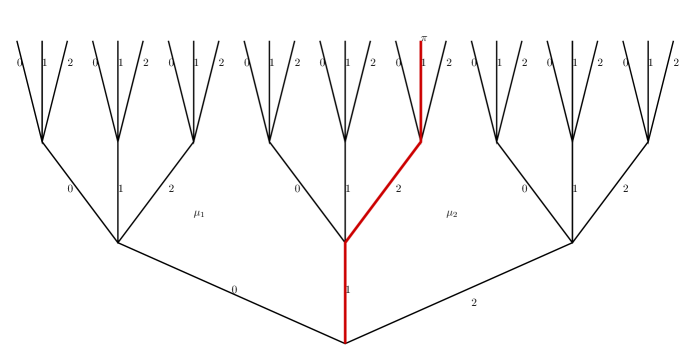
Figure 1. Half Cayley tree of order three. The bold path $\pi$ has representation by sequence $121\dots$. On the left (resp. right) side of this path the distribution $\mu$ coincides with $\mu_{1}$ (resp. $\mu_{2}$).

For a fixed $x^{0}\in V^{0}$, called the root, we set

$$W_{n}=\{x\in V^{0}|d(x,x^{0})=n\},\qquad V^{0}_{n}=\bigcup_{m=0}^{n}W_{m}.$$

On the tree $\Gamma^{k}$ one can introduce a partial ordering, by saying that $y>x$ if there exists a path $x=x_{0},x_{1},...,x_{n}=y$ from $x$ to $y$ that “goes upwards”, i.e., such that $d(x_{m},x^{0})=d(x_{m-1},x^{0})+1,m=1,\,\dots,n.$ The set of vertices $V_{x}=\{y\in V^{0}|y\geq x\}$ and the edges connecting them form the semi-infinite tree $\Gamma^{k}_{x}$ “growing” from the vertex $x\in V^{0}$.

Let $p$ be a prime number. In this paper we consider the half Cayley tree of order $p$. Take an arbitrary (finite or infinite) path $x^{0}=x_{0}<x_{1}<x_{2}<\dots$ on $\Gamma_{0}^{p}$ starting from the point $x^{0}$. We can represent the path by a sequence $i_{0}i_{1}i_{2}\dots$, where $i_{n}=0,1,\dots,p-1$. Namely, we label by $l_{0}(x),l_{1}(x),\dots,l_{p-1}(x)$ the edges going upward from the vertex $x\in V^{0}$. Then the path $x^{0}=x_{0}<x_{1}<x_{2}<\dots$ can be assigned a sequence $i_{0}i_{1}\dots$ such that $\langle x_{n-1},x_{n}\rangle=l_{i_{n-1}}(x_{n-1})$, $n=1,2,\dots$; the sequence $i_{0}i_{1}i_{2}\dots$ unambiguously determines the path $x^{0}=x_{0}<x_{1}<x_{2}<\dots$.

A finite path $x^{0}=x_{0}<x_{1}<x_{2}<\dots<x_{n}=x$ of length $n$ determines a point $x\in W_{n}$. If the path $x^{0}=x_{0}<x_{1}<x_{2}<\dots<x_{n}=x$ is represented by the sequence $i_{0}i_{1}\dots i_{n}$, we assume that the vertex $x$ is also represented by this sequence (see Fig. 1).

Let $x,y\in W_{n}$, and let $x$ be represented by the sequence $i_{0}i_{1}\dots i_{n}$ and $y$ by $j_{0}j_{1}\dots j_{n}$, where $i_{0}=j_{0}$, $i_{1}=j_{1}$,…, $i_{m}=j_{m}$, but $i_{m+1}<j_{m+1}$ for some $m$. In this case, we write $x\prec y$. Similarly, for pathes $\pi_{1}$ represented by a sequence $i_{0}i_{1}\dots i_{n}...$ and $\pi_{2}$ represented by $j_{0}j_{1}\dots j_{n}...$, we write $\pi_{1}\prec\pi_{2}$ if $i_{0}=j_{0}$, $i_{1}=j_{1}$,…, $i_{m}=j_{m}$, but $i_{m+1}<j_{m+1}$ for some $m$.

Let $\pi=\{x^{0}=x_{0}<x_{1}<\dots\}$ be an infinite path, represented by the sequence $i_{0}i_{1}i_{2}\dots$. We assign the $p$-adic number

$$t=t(\pi)=\sum_{n=0}^{\infty}{i_{n}p^{n}},\ \ t\in\mathbb{Z}_{p}$$

to the path $\pi$. This assignment is a 1-1 correspondence. Moreover, the partial order $\prec$ on the set of paths can be used to obtain partial order on $\mathbb{Z}_{p}$: namely, for $t_{1},t_{2}\in\mathbb{Z}_{p}$ we write $t_{1}\prec t_{2}$ iff they correspond to $\pi_{1}$,$\pi_{2}$ with $\pi_{1}\prec\pi_{2}$.

3. Construction of distributions

Several examples of $p$-adic distributions are known: Haar’s, Mazur’s, Bernoulli’s distributions etc.[13]. Recently some periodic distributions were constructed in [24]-[26].

Here for any two $p$-adic distribution given on $\mathbb{Z}_{p}$, say $\mu_{1}$ and $\mu_{2}$, $\mu_{1}\neq\mu_{2}$ we construct a new distribution $\mu=\mu(\mu_{1},\mu_{2})$ defined on $\mathbb{Z}_{p}$.

Fix a path $\pi$ with representation $\pi=i_{0}i_{1}\dots$. Take $a\in\mathbb{Z}_{p}$. If there exists $m\geq 0$ such that $a$ has representation $a=i_{0}+i_{1}p+\dots+i_{m}p^{m}+a_{m+1}p^{m+1}+\dots$ with $a_{m+1}\neq i_{m+1}$, then we denote this $m$ by $m(a,\pi)$. We say that two pathes starting from $x^{0}$ has non-empty intersection if they have at least one common edge.

Theorem 2.

Let $\pi=\{x^{0}=x_{0}<x_{1}<\dots\}$ be an infinite path, represented by the sequence $i_{0}i_{1}i_{2}\dots$ and $\mu_{1}$, $\mu_{2}$ are given distributions on $\mathbb{Z}_{p}$ such that $\mu_{1}\neq\mu_{2}$,

$$\mu_{1}(a+(p^{n}))=\mu_{2}(a+(p^{n})),\forall n\leq m(a,\pi)+1,$$ (3.1)

then there is a distribution $\mu$ on $\mathbb{Z}_{p}$, which on the intervals is defined as follows

$$\mu(a+(p^{n}))=\left\{\begin{array}[]{lllll}\mu_{1}(a+(p^{n})),\ \ \mbox{if}\ \ \pi_{a}\prec\pi,\pi_{a}\cap\pi=\emptyset\ \ \mbox{or}\ \ \pi_{a}\cap\pi\neq\emptyset,\ \ n\leq m\\ \ \ \ \ \ \ \ \ \ \ \ \ \ \ \ \ \ \ \ \ \ \mbox{or}\ \ \pi_{a}\cap\pi\neq\emptyset,\ \ n\geq m+1,\,a_{m+1}<i_{m+1}\\ \mu_{2}(a+(p^{n})),\ \ \mbox{if}\ \ \pi\prec\pi_{a},\pi_{a}\cap\pi=\emptyset\ \ \mbox{or}\\ \ \ \ \ \ \ \ \ \ \ \ \ \ \ \ \ \ \ \ \ \ \ \pi_{a}\cap\pi\neq\emptyset,\ \ n\geq m+1,\,a_{m+1}>i_{m+1}\\ \end{array}\right.$$ (3.2)

where $m=m(a,\pi)$ and $\pi_{a}$ is the path representing $a\in\mathbb{Z}_{p}$ (see Fig. 1).

Proof.

Consider the following (all possible) cases:

Case I: $\pi_{a}\cap\pi=\emptyset$. In this case the path $\pi_{a}$ always remains on the “left side” (i.e. $a_{0}<i_{0}$) or always on the “right side” (i.e. $a_{0}>i_{0}$) from the path $\pi$. For any $n\geq 1$ and any $b=0,1,\dots,p-1$ the number $bp^{n}$ (present in formula (2.2)) makes contributions only on levels $n$, $n+1$, … of the branch $V_{a_{0}}$ growing from the vertex of the edge numbered by $a_{0}$, (where $a_{0}\neq i_{0}$) of the tree $\Gamma^{p}_{0}$. We note that $V_{a_{0}}$ does not intersect with $\pi$. Consequently we have $\pi_{a+bp^{n}}\cap\pi=\emptyset$. By definition of $\mu$ given in (3.2) in case $\pi_{a}\cap\pi=\emptyset$ and $\pi_{a+bp^{n}}\cap\pi=\emptyset$ for any $b=0,1,...,p-1$ one easily checks that $\mu$ always coincides with $\mu_{1}$ (or $\mu_{2}$), hence it satisfies the distribution relation (2.2).

In case $n=0$, the exists $b_{0}\in\{0,1,\dots,p-1\}$ such that $\pi_{a+b_{0}}\cap\pi\neq\emptyset$, i.e. $a+b_{0}=i_{0}+a_{1}p+...$, where $i_{0}$ is the first number in the presentation of $\pi$. In this case assuming $\pi_{a}\prec\pi$ the equality (2.2) can be written as

$$\mu_{1}(a+(p^{0}))=\sum\limits_{b=0}^{b_{0}}\mu_{1}(a+b+(p^{1}))+\sum\limits_{b=b_{0}+1}^{p-1}\mu_{2}(a+b+(p^{1})).$$ (3.3)

Since the equality (2.2) is true for $\mu_{1}$, the equality (3.3) is satisfied iff

$$\sum\limits_{b=b_{0}+1}^{p-1}\mu_{2}(a+b+(p^{1}))=\sum\limits_{b=b_{0}+1}^{p-1}\mu_{1}(a+b+(p^{1})).$$ (3.4)

The last equality is true by condition (3.1).

Let now $\pi\prec\pi_{a}$ then the equality (2.2) can be written as

$$\mu_{2}(a+(p^{0}))=\sum\limits_{b=0}^{b_{0}}\mu_{2}(a+b+(p^{1}))+\sum\limits_{b=b_{0}+1}^{p-1}\mu_{1}(a+b+(p^{1})).$$ (3.5)

Similarly as the case $\pi_{a}\prec\pi$ we obtain condition (3.4).

Case II: $\pi_{a}\cap\pi\neq\emptyset$. In this case there exists $m=m(a,\pi)\geq 0$ such that $a$ has representation $a=i_{0}+i_{1}p+\dots+i_{m}p^{m}+a_{m+1}p^{m+1}+\dots$ with $a_{m+1}\neq i_{m+1}$.

Subcase $n\geq m+2$: Since the path $a_{m+1}a_{m+2}\dots$ does not intersect with $\pi$, the equation (2.2) for $n\geq m+2$ is

$$\mu_{1}(i_{0}+i_{1}p+\dots+i_{m}p^{m}+a_{m+1}p^{m+1}+\dots+(p^{n}))=$$

$$\sum_{b=0}^{p-1}\mu_{1}(i_{0}+i_{1}p+\dots+i_{m}p^{m}+a_{m+1}p^{m+1}+\dots+bp^{n}+(p^{n+1})),\ \ \mbox{if}\ \ a_{m+1}<i_{m+1};$$

and

$$\mu_{2}(i_{0}+i_{1}p+\dots+i_{m}p^{m}+a_{m+1}p^{m+1}+\dots+(p^{n}))=$$

$$\sum_{b=0}^{p-1}\mu_{2}(i_{0}+i_{1}p+\dots+i_{m}p^{m}+a_{m+1}p^{m+1}+\dots+bp^{n}+(p^{n+1})),\ \ \mbox{if}\ \ a_{m+1}>i_{m+1}.$$

Since both $\mu_{1}$ and $\mu_{2}$ are distributions the last two equalities are true.

Subcase $n\leq m+1$: In this case by our condition (3.1) we have $\mu_{1}=\mu_{2}$, consequently, the distribution relation (2.2) is satisfied. ∎

The following theorem says that one can construct a new distribution using a collection of given distributions.

Theorem 3.

Let $k$ be a natural number. Assume for each $t\in W_{k}$ a distribution $\nu_{t}$ on $\mathbb{Z}_{p}$ is given and there exists an interval $c+(p^{n_{0}})$, $n_{0}\geq k$ such that $\nu_{t}(c+(p^{n_{0}}))\neq\nu_{s}(c+(p^{n_{0}}))$ for at least one pair $t\neq s$, $t,s\in W_{k}$. Then there exists a distribution $\mu^{(k)}=\mu^{(k)}[\nu_{t},t\in W_{k}]$ on $\mathbb{Z}_{p}$ which is different from $\nu_{t}$ for each $t\in W_{k}$.

Proof.

The distribution $\mu^{(k)}$ can be constructed as follows (see Fig. 2).

Figure 2. The half Cayley tree of order three. Case $k=1$, elements of $W_{1}$ are defined by $0,1,2$ and $\mu^{(1)}$ coincides with distribution $\nu_{i}$, on the $i$th branch, where $i=0,1,2$.

Case: $n\geq k$. Recall $V_{t}$ is the set of vertices in the semi-infinite tree $\Gamma^{p}_{t}$ growing from the vertex $t\in V^{0}$. In the case $n\geq k$ if $\pi_{a}\cap V_{t}\neq\emptyset$, for some $t\in W_{k}$ then $\pi_{a+bp^{n}}$ also remains in $V_{t}$ for any $b=0,1,\dots,p-1$. Therefore we define

$$\mu^{(k)}(a+(p^{n}))=\nu_{t}(a+(p^{n})),\ \ \mbox{if}\ \ \pi_{a}\cap V_{t}\neq\emptyset,$$ (3.6)

then

$$\mu^{(k)}(a+bp^{n}+(p^{n+1}))=\nu_{t}(a+bp^{n}+(p^{n+1})),\ \ \mbox{for each}\ \ b=0,1,\dots,p-1.$$

Since $\nu_{t}$ is a given distribution the equation (2.2) is satisfied.

Case: $n\leq k-1$. Without loss of generality we define $\mu^{(k)}(a+(p^{n}))$ only for $a$ which has the form

$$a=a_{0}+a_{1}p+\dots+a_{k-1}p^{k-1},$$

where $a_{i}\in\{0,1,\dots,p-1\}$. Note that the sequence $a_{0}a_{1}\dots a_{k-1}$ presents a unique point of $W_{k}$.

For $n=k-1$ define

$$\mu^{(k)}(a_{0}+a_{1}p+\dots+a_{k-1}p^{k-1}+(p^{k-1}))$$

$$=\sum_{b=0}^{p-1}\nu_{a_{0}a_{1}\dots a_{k-2}(a_{k-1}+b){\rm mod}\,p}(a_{0}+a_{1}p+\dots+[(a_{k-1}+b){\rm mod}\,p]p^{k-1}+(p^{k})).$$ (3.7)

Now using formula (3.7) we define (for $n=k-2$)

$$\mu^{(k)}(a_{0}+a_{1}p+\dots+a_{k-2}p^{k-2}+(p^{k-2}))$$

$$=\sum_{b=0}^{p-1}\mu^{(k)}(a_{0}+a_{1}p+\dots+[(a_{k-2}+b){\rm mod}\,p]p^{k-2}+(p^{k-1}))$$ (3.8)

Iterating this procedure we recurrently define

$$\mu^{(k)}(a_{0}+a_{1}p+\dots+a_{k-m}p^{k-m}+(p^{k-m}))$$

$$=\sum_{b=0}^{p-1}\mu^{(k)}(a_{0}+a_{1}p+\dots+[(a_{k-m}+b){\rm mod}\,p]p^{k-m}+(p^{k-m+1})),$$ (3.9)

where $m=2,3,\dots,k$.

From the equalities (3.6)-(3.9) it follows that $\mu^{(k)}(a+(p^{n}))$ satisfies (2.2) for any $a\in\mathbb{Z}_{p}$ and any $n\geq 0$. Therefore, by Theorem 2 it follows that $\mu^{(k)}$ can be uniquely extended to a $p$-adic distribution on $\mathbb{Z}_{p}$.

Now we show that $\mu^{(k)}$ is different from $\nu_{t}$ for any $t\in W_{k}$. Let us assume the converse, i.e. there exists $u\in W_{k}$ such that $\mu^{(k)}=\nu_{u}$. This means that for any $a\in\mathbb{Z}_{p}$ and any $n\in\mathbb{N}$ we have

$$\mu^{(k)}(a+(p^{n}))=\nu_{u}(a+(p^{n})).$$ (3.10)

For any $a\in\mathbb{Z}_{p}$ there exists $t_{a}\in W_{k}$ such that $\pi_{a}\cap V_{t_{a}}\neq\emptyset$. Consequently, from (3.6) and (3.10) we get

$$\mu^{(k)}(a+(p^{n}))=\nu_{t_{a}}(a+(p^{n}))=\nu_{u}(a+(p^{n})),\ \ n\geq k.$$ (3.11)

When $a$ runs arbitrary $t_{a}$ takes all values on $W_{k}$. Therefore from (3.11) we get that $\nu_{t}(a+(p^{n}))=\nu_{u}(a+(p^{n}))$, $n\geq k$ for any $t\in W_{k}$. But this is contradiction to the condition of theorem for $a=c$ and $n=n_{0}$. Thus it follows that $\mu^{(k)}\neq\nu_{t}$ for each $t\in W_{k}$. This completes the proof. ∎

Remark 2.

We note that the distribution $\mu^{(k)}$ mentioned in Theorem 3 is useful to construct two distributions $\mu_{1}$ and $\mu_{2}$ which satisfy the condition of Theorem 2. Indeed, let $k=1$ and $\pi=i_{0}i_{1}\dots$, consider $\nu_{0},\nu_{1}$ such that $\nu_{0}(c+(p^{n_{0}}))\neq\nu_{1}(c+(p^{n_{0}}))$, for some $n_{0}\geq 1$ and $\pi_{c}\cap\pi=\emptyset$. Define $\tilde{\nu}_{t}$, $t\in W_{1}$ by

$$\tilde{\nu}_{t}=\left\{\begin{array}[]{ll}\nu_{0},\ \ \mbox{if}\ \ t=i_{0}\\ \nu_{1},\ \ \mbox{if}\ \ t\neq i_{0}.\end{array}\right.$$

Take $\mu_{1}=\nu_{0}$ and $\mu_{2}=\mu^{(1)}[\tilde{\nu}_{t},t\in W_{1}]$, it is easy to check that $\mu_{1}\neq\mu_{2}$ and they satisfy the condition of Theorem 2.

In the $p$-adic integral theory one need to $p$-adic measure. Because integral of a continuous function calculated with respect to unbounded $p$-adic distribution may not exist (see [13] for details).

In the following theorem we give a conditions under which $p$-adic distributions mentioned in Theorems 2 and 3 become $p$-adic measures.

Theorem 4.

The following statements hold

• Distribution $\mu$, mentioned in Theorem 2, is bounded iff $\mu_{1}$ and $\mu_{2}$ are bounded.

• Distribution $\mu^{(k)}$, mentioned in Theorem 3, is bounded iff $\nu_{t}(a+(p^{n}))$ is bounded for each $t\in W_{k}$ and $n\geq k$.

Proof.

1) This is consequence of the equality (3.2).

2) Case $n\geq k$: In this case from (3.6) we get that $\mu^{(k)}$ is bounded iff $\nu_{t}$ is bounded for each $t\in W_{k}$.

Case $n\leq k-1$: Since the right hand side of (3.7) is sum of bounded terms (corresponding to the case $n=k$) the left hand side also should be bounded. Consequently, iterating of the recursions (3.7)-(3.9) one can see that $\mu^{(k)}$ is bounded iff $\nu_{t}(a+(p^{n}))$ is bounded for each $t\in W_{k}$ and $n\geq k$. ∎

References

- [1] Baxter R.J. Exactly Solved Models in Statistical Mechanics (Academic, London, 1982).
- [2] Beltrametti E.G., Cassinelli G., Quantum Mechanics and -adic Numbers,Found. Phys. 2, (1972), 1-7.
- [3] Bleher P.M., Ganikhodjaev N.N. On pure phases of the Ising model on the Bethe lattice. Theor. Probab. Appl. 35 (1990), 216-227.
- [4] Gandolfo G., Rozikov U.A., Ruiz J. On -adic Gibbs measures for hard core model on a Cayley tree. Markov Processes Related Fields. 18(4) (2012), 701-720.
- [5] Ganikhodjaev N.N., Mukhamedov F.M., Rozikov U.A., Phase Transitions in the Ising Model on over the -adic Number Field, Uzb. Mat. Zh., No. 4, (1998), 23-29.
- [6] Gras Georges, Mesures -adiques. (French) Théorie des nombres, Année 1991/1992, 107 pp., Publ. Math.Fac. Sci. Besançon, Univ. Franche-Comté, Besançon.
- [7] Georgii H.-O., Gibbs Measures and Phase Transitions (W. de Gruyter, Berlin, 1988).
- [8] Khamraev M., Mukhamedov F.M., Rozikov U.A. On the uniqueness of Gibbs measures for adic non homogeneous model on the Cayley tree. Letters in Math. Phys. 70 (2004), 17-28.
- [9] Khrennikov A. Yu., -Adic Valued Probability Measures, Indag. Math., New Ser. 7 (1996), 311-330.
- [10] Khrennikov A. Yu., -Adic Valued Distributions in Mathematical Physics (Kluwer, Dordrecht, 1994).
- [11] Khrennikov A. Yu., Mukhamedov F.M., Mendes J.F.F., On -adic Gibbs Measures of the Countable State Potts Model on the Cayley Tree, Nonlinearity 20, (2007), 2923-2937.
- [12] Khrennikov A. Yu., Yamada S., van Rooij A., The Measure-Theoretical Approach to -adic Probability Theory, Ann. Math. Blaise Pascal 6, (1999), 21-32.
- [13] Koblitz N., -Adic Numbers, -adic Analysis, and Zeta-Functions (Springer, Berlin, 1977).
- [14] Mukhamedov F.M. On the Existence of Generalized Gibbs Measures for the One-Dimensional -adic Countable State Potts Model. Proc. Steklov Inst. Math., 265 (2009), 165-176.
- [15] Mukhamedov F.M., Rozikov U.A., On Gibbs Measures of -adic Potts Model on the Cayley Tree, Indag. Math., New Ser. 15 (2004), 85-100.
- [16] Mukhamedov F.M., Rozikov U.A., On Inhomogeneous -adic Potts Model on a Cayley Tree, Infin. Dimens. Anal. Quantum Probab. Relat. Top. 8, (2005), 277-290.
- [17] Mukhamedov F.M., Rozikov U.A., Mendes J.F.F., On Phase Transitions for -adic Potts Model with Competing Interactions on a Cayley Tree, in -Adic Mathematical Physics: Proc. 2nd Int. Conf., Belgrade, 2005 (Am. Inst. Phys., Melville, NY, 2006), AIP Conf. Proc. 826, pp. 140-150.
- [18] Mukhamedov F.M., Saburov M., Khakimov O.N., On -adic Ising Vannimenus model on an arbitrary order Cayley tree. J. Stat. Mech., 2015, P05032.
- [19] Mukhamedov F.M., On dynamical systems and phase transitions for -state -adic Potts model on the Cayley tree. Math. Phys. Anal. Geom. 53 (2013), 49–87.
- [20] van Rooij A. C. M., Non-Archimedean Functional Analysis (M. Dekker, New York, 1978).
- [21] Rozikov U.A. Gibbs measures on Cayley trees. World Sci. Publ. Singapore. 2013, 404 pp.
- [22] Schikhof W.H., Ultrametric Calculus (Cambridge Univ. Press, Cambridge, 1984).
- [23] Shiryaev, A.N. Probability, 2nd ed. Graduate Texts in Mathematics, vol. 95. Springer, New York, 1996.
- [24] Tugyonov Z. T. On periodic p-adic distributions. p-Adic Numbers Ultrametric Anal. Appl. 5(3) (2013), 218–225.
- [25] Tugyonov Z.T. Periodicity of Bernulli’s distribution. Uzbek Math. Jour. 2 (2013), 107–111.
- [26] Tugyonov Z.T. Non Uniqueness of -adic Gibbs distribution for the Ising model on the lattice . Jour. Siber. Federal Univ. 9(1) (2016), 123- 127.
- [27] Vladimirov V.S., Volovich I. V., Zelenov E. V., -Adic Analysis and Mathematical Physics (Nauka, Moscow, 1994; World Sci., Singapore, 1994).