Whiz: A Fast and Flexible Data Analytics System

Abstract— Today’s data analytics frameworks are compute-centric, with analytics execution almost entirely dependent on the pre-determined physical structure of the high-level computation. Relegating intermediate data to a second class entity in this manner hurts flexibility, performance, and efficiency. We present Whiz, a new analytics framework that cleanly separates computation from intermediate data. It enables runtime visibility into data via programmable monitoring, and data-driven computation (where intermediate data values drive when/what computation runs) via an event abstraction. Experiments with a Whiz prototype on a large cluster using batch, streaming, and graph analytics workloads show that its performance is 1.3-2$\times$ better than state-of-the-art.

1 Introduction

Many important applications in diverse settings rely on analyzing large datasets, including relational tables, event streams, and graph-structured data. To analyze such data, several systems have been introduced [45, 14, 46, 38, 24, 39, 7, 33, 4, 40, 41]. These enable data parallel computation, where a job’s analysis logic is run in parallel on data shards spread across multiple machines in large clusters.

Almost all these systems, be they for batch [20, 45, 14], stream [46, 4] or graph processing [38, 24, 39], have their intellectual roots in MapReduce [20], a time-tested data parallel execution framework. While they have many differences, the systems share a key attribute with MapReduce, in that they are compute-centric (§2). Their focus, like MapReduce, is on splitting a job’s computational logic, and distributing it across tasks to be run in parallel. Like MapReduce, all aspects of the subsequent execution of the job are rooted in the job’s computational logic, and its task-level distribution, i.e., the job computation structure. These include the fact that the compute logic running inside tasks is static and/or predetermined; intermediate data is partitioned and routed to where it is consumed based on the compute structure; and dependent tasks are launched when a fraction of upstream tasks they depend on finish. These attributes of job execution are not related to, or driven by, the properties of intermediate data, i.e., how much and what data is generated. Thus, intermediate data is a second-class citizen.

Compute-centricity was a natural choice for MapReduce. Knowing job structure beforehand simplifies carving computational units to execute tasks. Compute centricity provided clean mechanisms to recover from failures – only tasks on a failed machine needed to be re-executed. Job schedulers became simple because of having to deal with static inputs, i.e., fixed tasks/dependency structures. While originally designed for batch analytics, frameworks for streaming and graph analytics have shown that compute-centricity can be applied broadly.

However, given the benefit of hindsight, is compute-centricity the right choice? Our experience with building cluster schedulers, query optimizers, and execution engines, has shown that atleast four impediments arise from compute-centricity (§2): (1) Intermediate data being an opaque entity means there is no way to adapt job execution based on runtime data properties. (2) Static parallelism and intermediate data partitioning inherent to compute-centric frameworks constrain adaptation to data skew and resource flux. (3) Execution schedules being tied to compute structure can lead to resource waste while tasks wait for input to become available. (4) Compute-based organization of intermediate data can result in storage hotspots and poor cross-job I/O isolation, and it curtails data locality. Thus, compute-centricity begets inflexibility, poor performance, and inefficiency, which hurts production applications and cluster deployments.

Instead of adopting point fixes to today’s systems and work within compute-centricity limitations, this paper seeks a ground-up redesign. We observe that the above limitations arise from (1) tight coupling between intermediate data and compute, and (2) intermediate data agnosticity. Our framework, Whiz, cleanly separates computation from all intermediate data. Intermediate data is written to/read from a separate distributed key-value datastore. The store offers programmable visibility – applications can provide custom routines for monitoring runtime data properties. An event abstraction allows the store to signal to an execution layer when an application’s runtime data values satisfy certain properties. Decoupling, monitoring, and events enable data-driven computation: based on data properties, Whiz decides what logic to launch in order to further process data generated, how many parallel tasks to launch, when/where to launch them, and what resources to allocate to tasks. We show that such data-driven computation helps improve performance, efficiency, isolation, and flexibility, across a range of different application domains.

We make the following contributions in designing Whiz: (1) We present scalable APIs for programmable intermediate data monitoring, and for applications leveraging events for data-driven actions. Our APIs balance expressiveness against overhead. (2) We show how to organize intermediate data from multiple jobs in the datastore so as to achieve data locality, fault tolerance, and cross-job isolation. Since obtaining an optimal data organization is NP-Hard, we develop novel heuristics that carefully trade-off among these objectives. (3) We develop novel iterative heuristics for the execution layer for data-driven task parallelism and placement. This minimizes runtime skew in data processed and lowers data shuffle cost. (4) We launch each task in a container whose size is late-bound to the actual data allocated to the task, ensuring low data processing skew and optimal efficiency under resource dynamics.

We have built a Whiz prototype by modifying Tez [43] and YARN [47] ($15$K LOC). We currently support batch, graph, and stream processing. We deploy and experiment with our prototype on a 50 machine cluster in CloudLab [6]. We compare against several state-of-the-art compute centric (CC) approaches. Whiz improves median ($95\%$-ile) job completion time (JCT) by $1.3-1.6\times$ ($1.5-2.2\times$) across batch, streaming, and graph analytics. Whiz reduces idling by launching (the right number of appropriately-sized) tasks only when custom predicates on input data are met, and avoids expensive data shuffles even for consumer tasks. Under high cluster load, Whiz offers $1.8\times$ better JCT than CC due to better cross-job data management and isolation. Whiz’s data-driven actions enable computation to start much sooner than CC, leading to $1.3-1.6\times$ better stream and graph analytics median JCTs.

2 Compute-Centric Vs. Data-Driven

We begin with a brief overview of today’s batch, stream and graph processing systems (§2.1). We then discuss the three key design principles of Whiz (§2.2). Finally, we list the performance issues arising from compute-centricity and show how the data-driven design adopted by Whiz overcomes them (§2.3).

2.1 Today: Compute-Centric Frameworks

Production batch [52, 20, 5], stream [4, 52, 10] or graph [23, 38, 24] analytics frameworks support the execution of multiple interdependent stages of computation. Each stage is executed simultaneously within different tasks, each processing different data shards, or partitions, to generate input for a later stage.

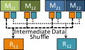
(a)

(b)

Figure 1: Simplified examples of existing analytics systems

Fig. 1a is an example of a simple batch analytics job. Here, two tables need to be filtered based on provided predicates and joined to produce a new table. There are 3 stages: two maps for filtering and one reduce to perform the join. Execution proceeds as follows: (1) Map tasks from both the stages execute first with each task processing a partition of the corresponding input table. (2) Map intermediate results are written to local disk by each task, split into files, one per consumer reduce task. (3) Reduce tasks are launched when the map stages are nearing completion; each reduce task shuffles relevant intermediate data from all map tasks’ locations, and generates output.

A stream analytics job (e.g., Fig. 1b) has a similar model [10, 34, 53]; the main difference is that tasks in all stages are always running. A graph analytics job, in a framework that relies on the popular message passing abstraction [38], has a similar but simplified model: the different stages are iterations in a graph algorithm, and thus all stages execute the same processing logic (with the input being the output of the previous iteration).

As the above shows, today’s frameworks are designed primarily with the goal of splitting up and distributing computation across multiple machines, making them compute centric (§1). Intermediate data is a second class citizen, strewn across many files at the locations where producer tasks are run, and routed along predetermined edges between producer and consumer tasks.

2.2 Whiz: A Data-Driven Framework

Whiz makes intermediate data a first class citizen (Fig. 3). It achieves this by adopting three design principles:

Decoupling compute and data: Whiz decouples compute from intermediate data (§4). Data from all stages across all jobs is written to/read from a separate key-value (KV) datastore, and managed by a distinct data management layer called the data service (DS). An execution service (ES) manages compute tasks.

Programmable data visibility: The above separation also enables low-overhead approaches to gain visibility into all runtime data (§5.1). A programmer can gather custom runtime data properties via a simple API.

Data-driven computation: Building on data visibility, Whiz provides an API for applications to act on events. Events form the basis for an intermediate data publish-subscribe substrate. Programmers can define custom predicates on intermediate data properties for each stage, and events notify the application when intermediate data satisfies the predicates. Events help achieve data-driven computation: properties of intermediate data drive all aspects of further computation (§5.2).

2.3 Overcoming Issues with Compute-centricity

We contrast Whiz with compute centricity along flexibility, performance, efficiency, placement, and isolation.

Data opacity, and compute rigidity: In compute-centric frameworks, there is no visibility into intermediate data generated by different stages of a job and the tasks’ computational logic are decided apriori. This prevents adapting the tasks’ logic based on their input data. Consider the job in Fig. 1a. Existing frameworks determine the type of join for the entire reduce stage based on coarse statistics [3]; unless one of the tables is small, a sort-merge join is employed to avoid out-of-memory (OOM) errors. On the other hand, having per-key histograms of intermediate data would enable dynamically determining the type of join to use for different reduce tasks. A task can use hash join if the total size of its key range is less than the available memory, and merge join otherwise. Whiz offers visibility into all intermediate data to support computation of such rich statistics which can be used to decide the logic to apply.

Static Parallelism, Partitioning: Today, jobs’ per-stage parallelism, inter-task edges and intermediate data partitioning strategy are decided independent of runtime data and resource dynamics. In Spark [52] the number of tasks in a stage is determined apriori by the user application or by SparkSQL [9]. A hash partitioner is used to place an intermediate $(k,v)$ pair into one of $|tasks|$ buckets. Pregel [38] vertex-partitions the input graph; partitions do not change during the execution of the algorithm.

This limits adaptation to resource flux and data skew. A running stage cannot utilize newly available compute resources [37, 26, 27] and dynamically increase its parallelism. If some key (or some vertex program) in a partition has an abnormally large number of records (or messages) to process then the corresponding task is significantly slowed down [13], affecting both stage and overall job completion times. Data skew is hard to predict.

With Whiz, because runtime data is managed independently (§4), compute and parallelism for downstream stages can be late-bound (§6.1). Based on the actual volume of runtime data, and the current resources, we determine how many tasks to launch and how to provision them. This controls data skew, and provisions task resources proportional to the data to be processed.

Idling due to compute-driven scheduling: Modern schedulers [47, 22] decide when to launch tasks for a stage based on the static computation structure. When a stage’s computation is commutative+associative, schedulers launch its tasks once 90% of all tasks in upstream stages complete [5]. But the remaining 10% producers can take long to complete [13] resulting in tasks idling.

Idling is worse in streaming, where consumer tasks are continuously waiting for data from upstream tasks. E.g., consider the streaming job in Fig. 1b. Stage 2 computes and outputs the median for every 100 records received. Between computation, S2’s tasks stay idle. As a result, the tasks in the downstream S3 stage also lay idle. To avoid idling, tasks should be scheduled only when, and only as long as, relevant input is available. Above, computation should be launched only after $\geq 100$ records have been generated by an S1 task.

Likewise, in batch analytics, if computation is commutative+associate, it is beneficial to “eagerly” launch tasks to process intermediate data whenever enough data has been generated to process in one batch, and exit soon after done. This is challenging to achieve today due to compute-driven scheduling and lack of data visibility.

Idling is easily avoided with Whiz: programmable monitoring aids runtime data statistics collection; when statistics indicate that relevant data has been generated, events are triggered, aiding launch of relevant tasks.

Placement, and storage isolation: Because intermediate data is spread across producer tasks’ locations, it is impossible to place consumer tasks in a data-local fashion. Such tasks are placed at random [20] and forced to engage in expensive shuffles that consume a significant portion of job run times ($\sim$30% [19]).

Also, when tasks from multiple jobs are collocated, it becomes difficult to isolate their hard-to-predict runtime intermediate data I/O. Tasks from jobs generating large intermediate data may occupy much more local storage and I/O bandwidth than those generating less.

Since the Whiz store manages data from all jobs, it can enforce policies to organize data to meet per-job objectives, e.g., data locality for any stage (not just input-reading stages), and to meet cluster objectives, such as I/O hotspot avoidance and cross-job isolation.

2.4 Related Work

Data opacity:

Almost all database and bigdata SQL systems [11, 49, 9] use statistics computed ahead of time to optimize execution. Adaptive query optimizers (QOs) [21] use dynamically collected statistics and re-invoke the QO to re-plan queries top-down. In contrast, Whiz alters the query plans on-the-fly at the execution layer based on run-time data properties, thereby circumventing additional expensive calls to the QO. Optimus [30] allows changing application logic based on approximate statistics operators that are deployed alongside tasks. However, the system targets simple computation logic rewriting, and cannot enable other data-driven benefits, e.g., adapting parallelism, and rightsizing tasks.

Skew handling and static parallelism: Some parallel databases [31, 25, 50] and big data systems [35] dynamically adapt to data skew for single large joins. In contrast, Whiz holistically solves data skew for all joins across multiple jobs and further strives to achieve data locality. [35, 25] deal with skew in MapReduce by dynamically splitting data for slow tasks into smaller partitions and processing them in parallel. But, they can cause additional data movement from already slow machines leading to poor performance. [15] mitigates skew by cloning slow tasks and adaptively partitioning work. However, it has no data visibility and its data organization does not consider data locality and fault tolerance.

Decoupling: Naiad [40] and StreamScope [48] also decouple intermediate data. They tag intermediate data with vector clocks which are used to trigger compute in the correct order. Thus, both support ordering driven computation, orthogonal to data-driven computation in Whiz. Also, Naiad assumes entire data fits in memory. StreamScope is not applicable to batch/graph analytics.

Storage inefficiencies: For batch analytics, [42, 29] addresses storage inefficiencies by pushing intermediate data to the appropriate external data services (like Amazon S3, Redis) while remaining cost efficient and running on serverless platforms. Similarly, [32] is an elastic data store used to store intermediate data of serverless applications. However, since this data is still opaque, and compute and storage are managed in isolation, these systems cannot support data-driven computation or achieve data locality and load balancing simultaneously.

3 Whiz Programming Model

	API	Description
1	createJob(name:Str, type:Type)	Creates a new job which can be of type BATCH, STREAM or GRAPH.
2	createStage(j:Job, name:Str, impl:StageImpl, trigger:StageDataReadyTriggerImpl)	Adds a stage of computation to a Job with a custom implementation. Optionally, users can specify custom predicates that determine when downstream stages can consume current stage’s data through StageDataReadyTriggerImpl. Otherwise default triggers are applied depending on job type.
3	addDependency(j: Job, s1: Stage, s2: Stage)	Adds a starts before relationship between stages s1 and s2.
4	addModifyAction(j:Job, s:Stage, impl:ModifyImpl)	Changes stage computation logic as specified by ModifyImpl. ModifyImpl is called when a statEvent arrives to rewrite job description.
5	replaceStage(j:Job, s:Stage, impl:AlterStageImpl)	Replaces stage implementation with an alternative implementation logic
6	addDataMonitor(j:Job, s:Stage, impl:DataMonitorImpl)	Adds a data monitor to compute statistics over data generated by stage s. DataMonitorImpl can either be a built-in module or a customized one.

Table 1: Whiz Programmer APIs.

Figure 2: An example three-stage job in Whiz

Whiz extends the DAG-based programming model of existing frameworks [20, 43, 10, 38] in a few key ways to support data-driven computation. Contrary to existing frameworks, Whiz does not require users to provide low-level details such as stage parallelism and data partitioning strategy. The minimal embellishment to familiar DAG-based programming, and freedom from low level details, ensure that Whiz is simple to program atop.

In Whiz, using the $addDataMonitor$ API (Table. 1 row 6), a user can add a built-in or custom module that computes statistics over data generated by a stage in a data-parallel program. Using the $createStage$ API (Table. 1 row 2), a user can provide predicates on the collected data properties ($StageDataReadyTriggerImpl$) to determine when a downstream stage can consume the current stage’s data. Using the $addModifyAction$ API (Table. 1 row 4), computation logic can be changed at runtime based on data properties.

As an example, consider a 3-stage job that processes words and, for words with $<500$ occurrences, sorts them by frequency. The program structure is $S_{1}\rightarrow S_{2}\rightarrow S_{3}$, where $S_{1}$ processes input words, $S_{2}$ computes word occurrences, and $S_{3}$ sorts the ones with $<500$ occurrences. In Whiz it can be realized as shown in Fig. 2. Job composition details (lines 1-6) are similar to existing frameworks. We specify the implementation of TriggerImpl for $S_{1}$ and ModifyImpl for $S_{3}$ that help realize data-driven computation. TriggerImpl specifies that as soon as 100 occurrences of a word are seen, $S_{2}$ can start running (lines 14-18), facilitating pipelined execution of $S_{1}$ and $S_{2}$. With the ModifyImpl for $S_{3}$ (lines 9-13), if the data consists of only words $\geq 500$ occurrences, then $S_{3}$ doesn’t need to execute (compute is replaced by null operation).

In Appendix. A, we show several other example applications written in Whiz. Our prototype supports batch SQL analytics, graph algorithms, and streaming.

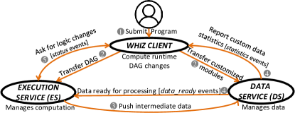
Figure 3: Whiz control flow.

The overall control flow in Whiz is shown in Fig. 3. The user program is provided to the Whiz client. The execution service (ES) runs the root vertex and writes its output to the datastore (step 3). The Data Service (DS) stores the received data and notifies ES when data is ready for further processing via an event (step 4). DS sends data statistics (e.g., per-key counts above) to Whiz client via events as well (step 4). On receiving a data-ready event, the ES (step 5) queries the client for compute changes. The above process repeats. Interactions between the ES, DS, and the client are hidden from the user.

4 Data Store

In Whiz, all jobs’ intermediate data is written to/read from a separate data store, where it is structured as $<$key,value$>$ pairs. In batch/stream analytics, the keys are generated by the stage computation logic itself; in graph analytics, keys are identifiers of vertices to which messages (values) are destined for processing in the next iteration. We now address how this data is organized in the store by the data service (DS). The DS does this organization via a cluster-wide master (DS-M).

An ideal data organization should achieve three cross- and per-job goals: (1) it should load balance and spread all jobs’ data, specifically, avoid hotspots and improve cross-job isolation, and minimize within-job skew in tasks’ data processing. (2) It should maximize job data locality by co-locating as much data having the same key as possible. (3) It should be fault tolerant - when a storage node fails, recovery should have minimal impact on job runtime. Next, we describe our data storage granularity, which forms the basis for meeting our goals.

4.1 Capsule: A Unit of Data in Whiz

Whiz groups intermediate data based on $<$key$>$s into groups called capsules. A stage’s intermediate data is organized into some large number $N$ capsules; crucially $N$ is late-bound as described below, which helps meet our goals above. Intermediate data key range is split $N$-ways, and each capsule stores all $<$k, v$>$ data from a given range. Whiz strives to materialize all capsule data on one machine; rarely, a capsule may be spread across a small number of machines. This materialization property of capsules forms the basis for consumer task data locality. In contrast, in today’s systems, data from the same key range may be written at different producers’ locations.

Also, today, key ranges of the intermediate data partitions are tied to pre-determined task parallelism, whereas Whiz capsule key ranges are unrelated to compute structure and late-bound. Specifically, we first determine the set of machines on which capsules from a stage are to be stored; machines are chosen to maximize the ability to simultaneously support isolation, load balancing, locality, and fault tolerance; the choice of machines then determines the number $N$ for a stage’s capsules (§4.2).

Given these machines and $N$, as the stage produces data at run time, $N$ capsules are materialized, and dynamically allocated to right-sized tasks; this is done in a way that preserves data-local processing, lowers skew, and optimally uses compute resources (§6).

Thus late-binding realizes an objectives-driven partitioning and consumption of intermediate data.

4.2 Fast Capsule Allocation

We consider how to place multiple jobs’ capsules on machines to avoid hotspots, ensure data locality and minimize job runtime impact on data loss. We formulate a binary integer linear program (see Fig. 11 in Appendix.  B) to this end. Solving this ILP at scale can take several tens of seconds delaying capsule placement.

Whiz instead uses a simpler, practical approach for the capsule placement problem. First, instead of jointly optimizing global placement decisions for all the capsules, Whiz solves a “local” problem of placing capsules for each stage independently (while still considering inter-stage dependencies); when new stages arrive, or when existing capsules may exceed job quota on a machine, new locations for some of these capsules are determined. Second, instead of solving a multi-objective optimization, Whiz uses a linear-time rule-based heuristic to place capsules; the heuristic prioritizes load and locality (in that order) in case machines satisfying all objectives cannot be found. Isolation (quota) is always enforced.

	// $Q_{j}$: $\max$ storage quota per job $j$ and machine $m$. Based on fairness considerations across all runnable jobs $J$.
	// $M_{v}$: number machines (out of $M$) to organize data that will be //generated by $v$ of $j$.
	a. Count number machines $M_{j75}$ where $j$ is using $<75\%$ of $Q_{j}$; b. $M_{v}$ = $max(2,M_{j75}\times\frac{M_{-}M_{j75}}{M})$.
	// Given $M_{v}$, compute list of machines $\overrightarrow{M_{v}}$ .
	Considers only machines where $j$ is using $<75\%$ of $Q_{j}$; a. Pick machines that provide LB, DL and maximum possible FT; b. If $|\overrightarrow{M_{v}}|$ $<M_{v}$, relax FT guarantees and pick machines that provide LB and DL; c. If $|\overrightarrow{M_{v}}|$ is still $<M_{v}$, pick machines that just provide LB.
	// Given $M_{v}$, compute total capsules N.
	$N$ = $G$ X $M_{v}$, where $G$ = capsules per machine
	// Which machines are at risk of violating $Q_{j}$?
	$\overrightarrow{M_{j}}$: machines which store data of $j$ and $j$ is using $\geq 75\%$ of $Q_{j}$.
	// Which capsules are hot on $\overrightarrow{M_{j}}$?
	Significantly larger in size or have a higher increasing rate than others.

Table 2: Heuristics employed in data organization

Capsule location for new stages: When a job $j$ is ready to run, DS-M invokes an admin-provided heuristic (Table 2) that assigns $j$ a quota $Q_{j}$ per machine.

When a stage $v$ of job $j$ starts to generate intermediate data, DS-M invokes to determine the number of machines $M_{v}$ for organizing $v$’s data. picks $M_{v}$ between $2$ and a fraction of the total machines which are $\leq 75\%$ of the quota $Q_{j}$ for $j$. $M_{v}\geq 2$ ensures opportunities for data parallel processing (§6.1); a bounded $M_{v}$ (Table 2) controls the ES task launch overhead (§6.1).

Given $M_{v}$, DS-M invokes to generate a list of machines $\overrightarrow{M_{v}}$ to materialize data on. It starts by creating three sub-lists: (1) For load balancing, machines are sorted lightest-load-first, and only ones which are $\leq 75\%$ quota usage for the corresponding job are considered. (2) For data locality, we prefer machines which already materialize other capsules for this stage $v$, or capsules from other stages whose output will be consumed by same downstream stage as $v$ (e.g., the two map stages in Fig. 1a). (3) For fault tolerance, we pick machines where there are no capsules from any of $v$’s $k$ upstream stages in the job, sorted in descending order of $k$. Thus, for the largest value of $k$, we have all machines that do not store data from any of $v$’s ancestors; for $k=1$ we have nodes that store data from the immediate parent of $v$.

We pick machines from the sub-lists to maximally meet our objectives in 3 steps: (1) Pick least loaded machines that are data local and offer as high fault tolerance as possible (machines present in all three sub-lists). Note that as we go down the fault tolerance list in search of a total of $M_{v}$ machines, we trade-off fault tolerance. (2) If despite reaching minimum fault tolerance as possible, i.e., reaching the bottom of the fault tolerance sub-list – the number of machines picked falls below $M_{v}$, we completely trade-off fault tolerance and pick least loaded machines that are data local (machines present in load balancing and data local sub-lists). (3) If still the number of machines picked falls below $M_{v}$, we trade-off data locality and simply pick least-loaded machines.

Finally, given $\overrightarrow{M_{v}}$, DS-M invokes and instantiates a fixed number ($G$) of capsules per machine leading to total capsules per-stage ($N$) to be $G\times M_{v}$. While a large G would aid us in better handling of skew and computation as the capsules can be processed in parallel, it comes at the cost of significant scheduling and storage overheads. We empirically study the sensitivity to $G$ (in §9.4); based on this, our prototype uses $G=24$.

New locations for existing capsules: Data generation patterns can significantly vary across different stages, and jobs, due to heterogeneous compute logics and data skew. Thus a job $j$ may run out of its quota $Q_{j}$ on machine $m$, leaving no room to grow already-materialized capsules of $j$ on $m$. Thus, DS-M periodically reacts to runtime changes by determining, $\forall j$: (1) which machines are at risk of being overloaded; (2) which capsules on these machines to spread at other locations; and (3) on which machines to them spread to.

Given a job $j$, DS-M invokes to determine machines where $j$ is using $\geq 75\%$ of its quota $Q_{j}$. DS-M then starts closing some capsules of $j$ on these machines; future intermediate data for these is materialized on another machine, thereby mitigating potential hotspots. Specifically, DS-M invokes to pick capsules that are either significantly larger in size or have a higher size increase rate than others for $j$ on $m$. These capsules are more likely to dominate the load and potentially violate $Q_{j}$. Focusing on them bounds the number of capsules that will spread out. DS-M groups the capsules selected based on the stage which generated them, and invokes heuristic as before to compute the set of machines where to spread. Grouping helps to maximize data locality, and provides load balance and fault tolerance.

5 Data Visibility

We now describe how Whiz offers run-time programmable data monitoring (§5.1), and data-driven computation using events (§5.2).

5.1 Data Monitoring

Whiz consolidates a capsule at one or a few locations (§4.1). Thus, capsules can be analyzed in isolation, simplifying data visibility. We achieve scalable monitoring via per-job masters (DS-JMs) which track light-weight stats at the capsule-level.

Whiz supports both built-in and customizable modules that periodically gather statistics per capsule, spanning properties of keys and values. These statistics are carried to the DS-JM where they are aggregated before being used by ES to take further data-driven actions (§5.2).

Built-in modules constantly collect light-weight statistics such as current capsule size, number of (k,v) pairs and rate of growth; in addition to supporting user programs, these are used by the store in runtime data organization (§4.2). Custom modules are UDFs (user defined functions). Since supporting arbitrary UDFs can impose high overhead, we restrict UDFs to those that can execute in linear time and O(1) state. We provide a library of common UDFs, such as computing the number of entries for which values are $<,=,$ or $>$ than a threshold.

5.2 Acting on Monitored Data Properties

Whiz supports data-driven computation via two key abstractions - events and ready triggers. The decoupled data and execution services interact with each other via events which trigger, and track progress of, data-driven computation. Ready triggers enable the DS-JM to decide when capsules can be deemed ready for corresponding computation to be run on them.

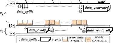
Figure 4: Data-driven computation facilitated by Whiz events. (1) Intermediate data ($v_{1}$) batches sent from ES to DS. (2) DS detects that 2 capsules are ready and sends data_ready event from DS to ES leading to downstream computation ($v_{2}$). (3) ES sends data_generated event to DS when entire output of $v_{1}$ pushed to DS. (4) DS sends data_ready_all event to ES indicating that all data_ready events have been sent.

Events: Whiz introduces 3 types of events: (1) A $data\_ready$ event is sent by the DS-JM to the ES whenever a capsule becomes ready (as per the ready trigger definition) to trigger corresponding computation. (2) A $data\_generated$ event is sent by the ES to the DS-JM when a stage in the user program finishes generating all its intermediate output. This event is required because in Whiz the DS-JM is unaware of the number of tasks that the ES launches corresponding to a stage, and thus cannot determine when a stage is completed. (3) A $data\_ready\_all$ event is sent by the DS-JM to the ES when a stage has generated all its intermediate data which is ready to be consumed by an immediate downstream stage. This event is required as the ES is unaware of the status of capsules (the total number of capsules, and whether they are done being materialized).

The use of these events is exemplified in Fig. 4. Here: when a stage $v_{1}$ generates a batch of intermediate data, a $data\_spill$ containing the data is sent to the data store, which accumulates it into capsules ($t_{0}$ through $t_{m}$). Whenever the DS-JM determines that a collection of $v_{1}$’s capsules (2 capsules in Fig. 4 at $t_{n}$) are ready for further processing, it sends a $data\_ready$ event per capsule to the ES; the ES could launch tasks of a consumer stage $v_{2}$ to process such capsules. This event carries per-capsule information such as: a list of machine(s) on which each capsule is spread, and a list of (aggregated) statistics (counters) collected by the built-in data modules. Finally, a $data\_generated$ event – from the ES, generated upon $v_{1}$ computation completing – notifies the DS-JM that $v_{1}$ finished generating $data\_spills$. Subsequently, DS-JM notifies the ES via the $data\_ready\_all$ event, that all capsules corresponding to $v_{1}$ have sent their data_ready events and have completely materialized (at $t_{m}$). This enables the ES to determine when the immediate downstream stage $v_{2}$, that is reading the data generated by $v_{1}$, has received all of its input data.

Triggers: The interaction between ES and DS via events is enabled by triggers whose logic is based on statistics collected by the data modules. A Whiz program can provide custom ready triggers for each job stage, which the Whiz client transfers to the DS-JM. Whiz also implements a default ready trigger which is otherwise applied.

Default ready trigger: Here, the DS-JM deems capsules ready when the computation generating them is done; this is akin to a barrier in batch systems today and bulk synchronous execution in graph analytics. For a streaming job, the DS-JM deems a capsule ready when it has $\geq X$ records ($X$ is a system parameter that a user can configure) from producer tasks, and sends a $data\_ready$ event to ES. On receiving this, ES executes a consumer stage task on this capsule. This is akin to micro-batching in existing streaming systems [53], with the crucial difference that the micro-batch is not wall clock time-based, but is based on the more natural intermediate data count.

Custom ready trigger: If available, the DS-JM deems capsules as ready using custom triggers. Programmers define these triggers based on knowledge about the semantics of the computation performed, and the type of data properties sought.

Consider the partial execution of a batch (or graph) analytics job, consisting of the first two logical stages (likewise, first two iterations) $v_{1}\rightarrow v_{2}$. If the processing logic in $v_{2}$ contains commutative+associative operations (e.g., sum, min, count, etc.), it can start processing its input before all of it is in place. For this, the user can define a pipelining ready trigger, and instruct DS-JM to consider a capsule generated by $v_{1}$ ready whenever the number of records in it reaches a threshold $X$. This enables the ES to overlap $v_{2}$’s computation with $v_{1}$’s data generation as follows: (1) Upon receiving a $data\_ready$ event from the DS-JM for capsules which have $>X$ records, the ES launches tasks of $v_{2}$. (2) Tasks read the current data, compute the associative+commutative function on the (k,v) data read, and push the result back to data store (in the same capsules advertised through the received $data\_ready$ event). (3) The DS-JM waits for each capsule to grow back beyond threshold $X$ for generating subsequent $data\_ready$ events. (4) Finally, when a $data\_generated$ event is received from $v_{1}$, the DS-JM triggers a final $data\_ready$ event for all the capsules generated by $v_{1}$, and a subsequent $data\_ready\_all$ event, to enable $v_{2}$’s final output to be written in capsules and fully consumed by a downstream stage, say $v_{3}$ (similar to Fig. 4). Such pipelining speeds up jobs in batch and graph analytics, as we show in  §9.1.2.

The above pipelining ready trigger can be extended across capsules. E.g., the DS-JM could deem all capsules ready when the number of entries generated across all capsules crosses a threshold. In streaming, such triggers help improve efficiency and performance (§9.1.3). In a two-stage streaming job $v_{1}\rightarrow v_{2}$, $v_{2}$ may (re)compute a weighted moving average whenever $100$ data points with distinct keys are generated by $v_{1}$. A pipelining trigger can be used to signal all $v_{1}$ capsules as ready once said threshold is met. This brings data driven-ness to stream analytics: computation is performed only when the required records have streamed into the system.

In a similar manner, we can trigger processing based on special records. Stream processing systems often rely on “low watermark” records to ensure event-time processing [18, 36], and to support temporal joins [36]. Custom triggers can be used to launch, on demand, temporal operators whenever a low watermark record is observed at any of a stage’s output capsules.

6 Execution Service

The ES launches a per-job master (ES-JM) which late-binds the job’s computation, i.e., given intermediate data ready for processing, and available resources, (a) it determines optimal parallelism and deploys tasks to minimize skew and shuffle, and (b) it maps capsules to tasks in a resource-aware fashion (§6.1). The ES-JM design naturally mitigates stragglers (§6.2), and facilitates data-driven compute logic changes (§6.3).

6.1 Task Parallelism, Placement, and Sizing

Given a set of ready capsules ($C$) for a stage, the ES-JM maps subsets of capsules to tasks, and determines the location (across machines $M$) and the size of the corresponding tasks based on available resources. This multi-decision problem, which evens out data volume processed by tasks in a stage, and minimizes shuffle subject to resource contraints on each machine, can be cast as a binary ILP (omitted for brevity). However, the formulation is non-linear; even a linear version is slow to solve at scale. For tractability, we propose an iterative procedure that applies a set of heuristics (Tab. 3) repeatedly until tasks for all ready capsules are allocated, and their locations and sizes (resources) determined.

	// $\overrightarrow{C}$: subsets of unprocessed capsules. a. $CaMax$ = $2\times|c|$, $c$ is largest capsule $\in$ $C$; b. Group all capsules $\in$ $C$ into subsets in strict order: i. data local capsules together; ii. each spread capsule, along data-local capsules together; iii. any remaining capsules together; subject to: iv. each subset size $\leq CaMax$; v. conflicting capsules don’t group together; vi. troublesome capsules always group together.
	// $\overrightarrow{M}$: preferred machines to process each subset $\in$ $\overrightarrow{C}$. c. no machine preference for troublesome subsets $\in$ $\overrightarrow{C}$ d. for every other subset $\in$ $\overrightarrow{C}$ pick machine $m$ such that: i. all capsules in the subset are only materialized at $m$; ii. otherwise $m$ contains the largest materialization of the subset.
	Compute $\overrightarrow{R}$: resources needed to execute each subset $\in$ $\overrightarrow{C}$: e. $\overrightarrow{A}$ = available resources for $j$ on machines $\overrightarrow{M}$; f. $F$ = $\min{(\frac{\overrightarrow{A}[m]}{\text{total size of capsules{} allocated to $m$}}}$, for all $m\in\overrightarrow{M}{)}$; g. for each subset $i\in\overrightarrow{C}$:         $\overrightarrow{R}[i]$ = $F\times\text{total size of capsules{} allocated to $\overrightarrow{C}[i]$}$.

Table 3: Heuristics to group capsules and assign them to tasks

The iterative procedure consists of 3 steps - (a) generate optimal subsets of capsules to minimize cross-subset skew (using ), (b) decide on which machine should a subset be processed to minimize shuffle ( ), and (c) determine resources required to process each subset ( ).

First, we group capsules, $C$, into a collection of subsets, $\overrightarrow{C}$, using . We then try to assign each group to a task. Our grouping into subsets attempts to ensure that data in a subset is spread on just one or a few machines (lines (b.i-b.iii)), which minimizes shuffle, and that the total data is spread roughly evenly across subsets (line (b.iv)) making cross-task performance uniform. We place a bound $CaMax$, equaling twice the size of the largest capsule, on the total size of a subset (see line (a)). This bound ensures that multiple (atleast 2) capsules are present in each subset, which helps in mitigating stragglers (§6.2).

Second, we determine a preferred machine to process each subset using ; this is a machine where most if not all capsules in the subset are materialized (line (d)). Choosing a machine in this manner minimizes shuffle.

Finally, given available resources across the preferred machines (from the cluster-wide resource manager [47]) we need to allocate tasks to process subsets. But some machines may not have resource availability. For the rest of this iteration, we ignore such machines and the subsets of capsules that prefer such machines.

Given machines with resources $\overrightarrow{A}$, we assign a task for each subset of capsules which can be processed, and allocate task resources altruistically using . That is, we first compute the minimum resource available to process unit data ($F$; line (f)). Then, for each task, the resource allocated (line (g)) is $F$ times the total data in the subset of capsules allocated to the task ($|\overrightarrow{C}[i]|$).

Allocating resources proportional to input size coupled with roughly equal subset sizes, ensures that tasks have roughly equal finish times in processing their subsets of capsules. Furthermore, by allocating resources corresponding to the minimum available, our approach realizes altruism: if a job gets more resources than what is available for the most constrained subset, then it does not help the job’s completion time (because completion time depends on how fast the most constrained subset is processed). Altruistically “giving back” such resources helps speed up other jobs or other stages in the same job.

The above 3 steps repeat whenever new capsules are ready, or existing ones can’t be scheduled. Similar to delay scheduling [51], we attempt several tries to execute a group which couldn’t be scheduled on its preferred machine due to resource unavailability, before marking capsules conflicting. These are re-grouped in the next iteration (line (b.v)). Finally, capsules that cannot be executed under any grouping are marked troublesome (line (b.vi)) and processed on any machine (line (d.ii)).

6.2 Handling Stragglers

Data organization into capsules and late-binding computation to data enables a natural, simple, and effective straggler mitigation technique. If a task struck by resource contention makes slower progress than others in a stage, given that there are multiple capsules assigned to a task, the ES-JM simply splits the task’s capsule group into two, in proportion of the task’s processing speed relative to average speed of other tasks in the stage. It then assigns the larger-group capsules to a new task, and places the task using the approach above. This addresses stragglers via work reallocation, as opposed to using clone tasks [54, 13, 11, 35, 12] in compute-centric frameworks. Cloning waste resources and duplicates work.

6.3 Runtime DAG Changes

Visibility into data enables run-time changes to tasks’ logic. In Whiz, we introduce statistics and status events, defined next, to support this. Whenever a capsule is deemed ready, the DS-JM sends a statistics event to the Whiz client, which carries the capsule statistics. Status events help the ES-JM query the Whiz client to check if the user program requires alternate logic to be launched based on observed statistics.

Upon receiving data_ready events from the DS-JM, ES-JM sends status events to the Whiz client to determine how to process a given capsule. Given the user-provided compute logic and capsule statistics obtained through statistics events, the Whiz client notifies the ES to take one the following actions: (1) no new action – assign computation as planned; (2) ignore – don’t perform any computation, as the user program deemed the capsule to not have any useful data to compute on; (3) replace computation with new logic supplied by the user.

7 Fault Tolerance

Task Failure. When a Whiz task fails due to a machine failure, only the failed tasks need to be re-executed if the input capsules are not lost. However, this will result in duplicate data in all capsules for the stage leading to intermediate data inconsistencies. To address this, we use checksums at the consumer task-side Whiz library to suppress duplicate spills.

However, if the failed machine also contains the input capsules of the failed task, then the ES-JM triggers the execution of the upstream stage(s) to regenerate the input capsules of the failed task. Recall that Whiz’s fault tolerance-aware capsule storage (§4) helps control the number of upstream (ancestor) stages that need to be re-executed in case of data loss.

DS-M/DS-JM/ES-JM. Whiz maintains replicas of DS-M/DS-JM daemons using Apache Zookeeper [28], and fails over to a standby. Given that Whiz decides the task composition of a job at runtime in a data-driven manner, upon ES-JM failure, we simply need to restart it so that it can resume handling events from the DS. During this time already launched tasks continue to run.

8 Implementation

We prototyped Whiz by modifying Tez [5] and leveraging YARN [47]. Whiz’s core components are application agnostic and support diverse analytics as shown in §9.

The DS was implemented from scratch and consists of three kinds of daemons: cluster-wide master (DS-M) and per-job masters (DS-JM), which we discussed in earlier sections, and workers (DS-W). The DS-W runs on cluster machines and conducts node-level data management. It handles storing the data received from the ES or from other DS-Ws in a local in-memory file system (tmpfs [44]) and transfers data to other DS-Ws per DS-M directives. It collects statistics and reports to the DS-M/DS-JMs via heartbeats. Finally, it provides ACKs to ES tasks for the data they write. We use YARN to launch/terminate daemons.

The ES was implemented by modifying components of Tez to enable data-driven execution. ES tasks are modified Tez tasks that have an interface to the local DS-W as opposed to local disk or cluster-wide storage. The Whiz client is a standalone process per-job.

All communication (asynchronous) between DS, ES and Whiz client is implemented through RPCs in YARN using Google Protobuf [8]. We also use RPCs for communication between the YARN Resource Manager (RM) and ES-JM to propagate job resource allocation (§6).

9 Evaluation

We evaluated Whiz on a $50$-machine cluster deployed on CloudLab [6] using publicly available benchmarks – batch TPC-DS jobs, PageRank for graph analytics, and synthetic streaming jobs. Unless otherwise specified, we set Whiz to use default ready triggers, equal storage quota ($Q_{j}=2.5GB$) and 24 capsules per machine.

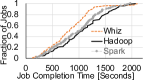
(a)

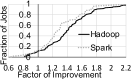
(b)

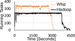
(c)

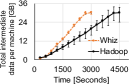
(d)

Figure 5: (a) CDF of JCT; (b) CDF of factors of improvement of individual jobs using Whiz w.r.t. baselines [2, 52]; (c) Running tasks; (d) Per machine average, min and max storage load.

9.1 Testbed Experiments, Different Applications

Workloads: We consider a mix of jobs, all from TPC-DS (batch), or all from PageRank (graph). In each experiment, jobs are randomly chosen and follow a Poisson arrival distribution with average inter-arrival time of 20s. Each job lasts up to 10s of minutes, and takes as input tens of GBs of data. For streaming, we created a synthetic workload from a job which periodically replays GBs of text data from HDFS and returns top 5 most common words for the first 100 distinct words found. We run each experiment thrice and present the median.

Cluster, baseline, metrics: Our machines have 8 cores, 64GB of memory, 256GB storage, and a 10Gbps NIC. The cluster network has a congestion-free core. We compare Whiz as follows: (1) Batch: vs. Tez [5] running atop YARN [47], for which we use the shorthand “Hadoop” or “CC”; and vs. SparkSQL [14]; (2) Graph: vs. Giraph (i.e., open source Pregel [38]); and vs. GraphX [24]; (3) Streaming: vs. SparkStreaming [53]. We study the relative improvement in the average job completion time (JCT), or Duration_CC/Duration${}_{{\textsc{\small Whiz}}}$. We measure efficiency using makespan. For a fair comparison with Hadoop and Giraph, we ensure that they use tmpfs.

9.1.1 Batch Analytics

Performance and efficiency: Fig. 5a shows the JCT distributions of Whiz, Hadoop, and Spark for the TPC-DS workload. Only $0.4$ ($1.2$) highest percentile jobs are worse off by $\leq 1.06\times$ ($\leq 1.03\times$) than Hadoop (Spark). Whiz speeds up jobs by $1.4\times$ ($1.27\times$) on average, and $2.02\times$ ($1.75\times$) at $95th$ percentile w.r.t. Hadoop (Spark). Also, Whiz improves makespan by $1.32\times$ ($1.2\times$).

Fig. 5b presents improvement for individual jobs. For more than $88\%$ jobs, Whiz outperforms Hadoop and Spark. Only $12\%$ jobs slow down to $\leq 0.81\times$ ($0.63\times$) using Whiz. Gains are $>1.5\times$ for $>35\%$ jobs.

Sources of improvements: We observe that more rapid processing, and better data management contribute most to benefits.

First, we snapshot the number of running tasks across all the jobs in one of our experiments when running Whiz and Hadoop (Fig. 5c). Whiz has $1.45\times$ more tasks scheduled over time which translates to jobs finishing $1.37\times$ faster. It has $1.38\times$ better cluster efficiency than Hadoop. Similar observations hold for Spark (omitted).

The main reasons for rapid processing/high efficiency are: (1) The DS (§4.2) ensures that most tasks are data local ($76\%$ in our expts). This improves average consumer task completion time by $1.59\times$. Resources thus freed can be used by other jobs’ tasks. (2) Our ES can provide similar input sizes for tasks in a stage (§6.1) – within $14.4\%$ of the mean (more in §9.2).

Second, Fig. 5d shows the size of the cross-job total intermediate data per machine. We see that Hadoop generates heavily imbalanced load spread across machines. This creates many storage hotspots and slows down tasks competing on those machines. Spark is similar. Whiz mitigates hotspots (§4) improving overall performance.

Whiz slowdown: We observe jobs generating less intermediate data are more prone to performance losses, especially under ample resource availability. A reason is that Whiz strives for capsule-local task execution (§6.1). If resources are unavailable, Whiz will assign the task to a data-remote node, or get penalized waiting for data-local placement. Also, Whiz gains are lower w.r.t. Spark. This is an artifact of our Hadoop-based implementation, and of using a non-optimized in-memory store.

Only $18\%$ of capsules across all jobs are spread across machines. Also, $>25\%$ of the jobs whose performance improves processed “spread-out” capsules; and $\leq 14\%$ of the slowed jobs processed spread capsules.

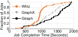
(a)

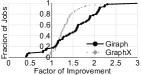
(b)

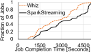
(c)

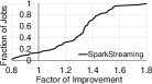
(d)

Figure 6: (a) CDF of JCT using Whiz, GraphX [24] and Giraph [1]; (b) CDF of factors of improvement of individual jobs using Whiz w.r.t. GraphX and Giraph; (c) CDF of JCT using Whiz and SparkStreaming [53]; (d) CDF of factors of improvement of individual jobs using Whiz w.r.t. SparkStreaming.

9.1.2 Graph Processing

We run multiple PageRank (40 iters.) jobs on the Twitter Graph [17, 16]. Whiz groups data (messages exchanged over algorithm iterations) into capsules based on vertex ID. We use a custom ready trigger (§5.2) so that a capsule is processed only when $\geq 1000$ entries are present.

Fig. 6a shows the JCT distribution of Whiz, GraphX and Giraph. Whiz speeds up jobs by $1.33\times$ ($1.57\times$) on average and $1.57\times$ ($2.24\times$) at the $95th$ percentile w.r.t. GraphX (Giraph) (Fig. 6b). Gains are lower w.r.t. GraphX, due to its efficient implementation atop Spark. However, $<10\%$ jobs are slowed down by $\leq 1.13\times$.

Improvements arise for two reasons. First, Whiz is able to deploy appropriate number of tasks only when needed: custom ready triggers immediately indicate data availability, and runtime parallelism (§6.1) allows messages to high-degree vertices [24] to be processed by more than one task. Also, Whiz has $1.53\times$ more tasks (each runs multiple vertex programs) scheduled over time; rapid processing and runtime adaptation to data directly leads to jobs finishing faster. Second, because of triggered compute, Whiz doesn’t hold resources for a task if not needed, resulting in $1.25\times$ better cluster efficiency.

9.1.3 Stream Processing

We configure the Spark Streaming micro-batch interval to 1 minute. With Whiz, we implemented a custom ready trigger to enable computation whenever $\geq 100$ distinct entries are present in the intermediate data. Figures 6c,  6d show our results. Whiz speeds up jobs by $1.33\times$ on average and $1.55\times$ at the $95th$ %-ile. Also, $15\%$ of the jobs are slowed down to around $0.8\times$.

The reason for gains is data-driven computation via custom ready triggers; Whiz does not have to delay execution till the next micro-batch if data can be processed now. A SparkStreaming task has to wait as it has no data visibility. In our experiments, more than $73\%$ executions happen at less than $40s$ time intervals with Whiz.

Whiz suffers due to implementation atop a non-optimized streaming stack. Launching tasks in YARN is significantly slower than acquiring tasks in Spark. This can be exacerbated by ES stickiness to data locality. However, this is amortized over long job run times.

9.1.4 Whiz Overheads

CPU, memory overhead: We find that DS-W (§8) processes inflate the memory and CPU usage by a negligible amount even when managing data close to storage capacity. DS-M and DS-JM have similar resource profiles.

Latency: We compute the average time to process heartbeats from various ES/DS daemons, and Whiz client. For $5000$ heartbeats, the time to process each is $2-5ms$. We implemented the Whiz client and ES-JM logic atop Tez AM. Our changes inflate AM decision logic by $\leq 14ms$ per request with negligible increase in AM memory/CPU.

Network overhead from events/heartbeats is negligible.

9.2 Benefits of Data-driven Computation

The overall benefits of Whiz above also included the effects of dynamic parallelism/placement/sizing (§6.1) and straggler mitigation (§6.2). We now delve deeper into them to shed more light on data-driven computation benefits during one of our TPC-DS runs.

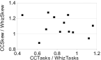
(a)

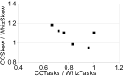
(b)

Figure 7: Fraction of tasks allocated by CC w.r.t. to Whiz vs. the fraction of skew among tasks due to CC w.r.t. Whiz, in a given stage: (a) for a job with $12$ stages where Whiz improves JCT by $1.6\times$; (b) for a job with $6$ stages, where Whiz improves JCT by $1.2\times$. $\frac{CCSkew}{WhizSkew}>1$ means Whiz has less skew; $\frac{CCTasks}{WhizTasks}<1$ means CC under-parallelize a given stage.

Skew and parallelism: Fig. 7 shows fractions of skew and parallelism as generated by CC w.r.t. Whiz for two TPC-DS jobs from one of our runs. Whiz’s ability to dynamically change parallelism at runtime, driven by the number of capsules for each vertex, leads to significantly less data skew than CC. When CC is under-parallelizing, the skew is significantly higher than Whiz (up to $1.43\times$). Over-parallelizing does not help either; CC incurs up to $1.15\times$ larger skew, due to its rigid data partitioning and tasks allocation schemes. Even when Whiz incurs more skew (up to $1.26\times$), corresponding tasks will get allocated more resources to alleviate this overhead (§6.1).

Straggler mitigation: We evaluated the benefits enabled by Whiz’s straggler mitigation strategy w.r.t. (1) the default speculative execution strategy from CC and (2) when there is no strategy. We slowdown the same set of $10\%$ of machines in the cluster for each run. Table 4b shows our results. Whiz’s straggler mitigation strategy improves JCT $1.47\times$ on average w.r.t. no strategy. This is because stragglers can significantly impact overall performance. However, even when the CC speculative execution strategy is enabled, Whiz performs $1.19\times$ better. This is due to its ability to reassign only the unprocessed input data to the speculative tasks instead of launching clones of the straggler tasks.

Additionally, we run microbenchmarks to delve further into Whiz’s data-driven benefits (results in Appendix C).

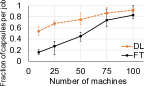
(a)

(b)

Figure 8: (a) Average, min and max fraction of capsules which are data local (DL) respectively fault tolerant (FT) across all the jobs for different cluster load; (b) Max, min and ideal storage load balance (LB) on every machine for different cluster load.

9.3 Load Balancing, Locality, Fault Tolerance

To evaluate DS load balancing (LB), data locality (DL) and fault tolerance (FT), we stressed the data organization under different cluster load. We used job arrivals and all stages’ capsule sizes from one of our TPC-DS runs.

The main takeaways are (Fig. 8): (1) Whiz prioritizes DL and LB over FT across cluster loads (§4.2); (2) when the available resources are scarce ($5\times$ higher load than initial), all three metrics suffer. However, the maximum load imbalance per machine is $<1.5\times$ than the ideal, while for any job, $\geq 47\%$ of the capsules are DL. Also, on average $16\%$ of the capsules per job are FT; (3) less cluster load ($0.6\times$ lower than initial) enables more opportunities for DS to maximize all of the objectives: $\geq 84\%$ of the per-job capsules are DL, $71\%$ are FT, with at most $1.17\times$ load imbalance per machine than the ideal.

% Machines	JCT [Seconds]
Failed	Avg	Min	Max
None	725	215	2100
10%	740	250	2320
25%	820	310	2360
50%	1025	350	2710
75%	1600	410	3300

(a)

Straggler	JCT [Seconds]
Strategy	Avg	Min	Max
None	1200	410	2750
Speculative	970	280	2300
Whiz	815	330	1920

(b)

Table 4: Whiz’s variation in JCT in the presence of: (a) random machines failures; (b) different straggler mitigation strategies; Speculative is the default approach used by CC and Whiz is our approach as described in  §6.2.

Failures: Using the same workload, we also evaluated the performance impact in the presence of machine failures (Table 4a). We observe that Whiz does not degrade job performance by more than $1.13\times$ even when $50\%$ of the machines fail. This is mainly due to DS’s ability to organize capsules to be FT across ancestor stages and avoid data recomputations. Even when $75\%$ of the machines fail, the maximum JCT does not degrade by more than $1.57\times$, mainly due to capsules belonging to some ancestor stages still being available, which leads to fast recomputation for corresponding downstream vertices.

9.4 Sensitivity Analysis

Impact of Contention: We vary storage load, and hence resource contention, by changing the number of machines while keeping the workload constant; half as many servers lead to twice as much load. We see that at $1\times$ cluster load, Whiz improves over CC by $1.39\times$ ($1.32\times$) on average in terms of JCT (makespan). Even at high contention (up to $4\times$), Whiz’s gains keep increasing $1.83\times$ ($1.42\times$). This is because data is load balanced leading to few storage hotspots, better isolation, and Whiz minimizes resource wastage and the time spent in shuffling.

Impact of $G$ (number of capsules per machine): We now provide the rationale for picking $G=24$. Table 5 shows the factors of improvements w.r.t. CC for different values of $G$ and levels of contention.

The main takeaways are as follows: for $G=8$ the performance gap between Whiz and CC is low ($<1.1x$). This is expected because small number of capsules results in less data locality (each capsule is more likely to be spread). Further, the gap decreases at high resource contention. In fact, at $4x$ the cluster load, CC performs better ($0.85x$). At larger values of $G$ the performance gap increases. For example, at $G=24$, its gains are the most (between $1.39x$ and $1.58x$). This is because larger $G$ implies (1) more flexibility for Whiz to balance the load across machines; (2) more likely that few capsules are spread out; (3) lesser data skew and more predictable per task performance. However, a very large $G$ does not necessarily improve performance, as it can lead to massive task parallelism. The resulting scheduling overhead degrades performance, especially at high load.

Multiple of	$\#$ Capsules
Original Load	8	16	20	24	28	32	36	40
1	1.07	1.33	1.46	1.52	1.57	1.63	1.54	1.46
2	1.10	1.16	1.53	1.58	1.56	1.61	1.47	1.31
4	0.85	1.12	1.34	1.39	1.32	1.16	0.95	0.74

Table 5: Factors of improvement w.r.t. CC for different number of capsules per machine and cluster load.

Altruism: Can altruistically deciding task sizing (§6) impact job performance? We compare Whiz’s approach with a greedy task sizing approach, where each task gets $\frac{1}{\#jobs}$ resource share per machine, and uses all of it. For the same workload as  §9.3, Whiz actually speeds up jobs by $1.48\times$ on avg., and $3.12\times$ ($4.8\times$) at $75th$ %-ile ($95th$ %-ile) w.r.t. greedy approach. Only $16\%$ jobs are slowed down by $\leq 0.6\times$. Altriusm, by late-binding resources with the slowest potential task, helps all jobs benefit.

10 Summary

The compute-centric nature of existing frameworks hurts flexibility, efficiency, isolation, and performance. Whiz reenvisions analytics frameworks by cleanly separating computation from intermediate data. Via programmable monitoring of data properties and a rich event abstraction, Whiz enables data-driven decisions for what computation to launch, where to launch it, and how many parallel instances to use, while ensuring isolation. Our evaluation using batch, stream and graph workloads shows that Whiz outperforms state-of-the-art frameworks.

Appendix A Whiz Sample Programs

A key advantage of Whiz is its programming model wherein users no longer have to provide low level details and gain the benefits of data-driven computation using our APIs. While we showed a sample batch analytics application earlier (§3), we now show how to write more diverse application atop Whiz. More specifically, we show how to write a graph analytics job and a stream processing job.

Figure 9: An example graph job in Whiz

Graph Analytics (Fig. 9). We consider the graph analytics application that we used in our testbed experiments (§9), .i.e., a job running the PageRank algorithm. Job composition details are similar to existing frameworks (lines 1-2). Similar to the $createStage$ API which is used for batch/stream jobs, we have a $loadGraph$ API which constructs the graph, given the input. Additionally, we specify the vertex program logic to run PageRank via the PageRankImpl function.

Crucially, Whiz allows a user to run the graph algorithm in a data-driven manner by specifying the implementation of TriggerImpl. TriggerImpl specifies that as soon as 1000 entries corresponding to a vertex are seen, then we trigger the execution of the vertex program, leading to pipelined execution (lines 4-8). The user instructs the DS to use the built-in module to collect the per-key counts (line 3). This simple yet powerful trigger naturally deals with high-degree vertices and leads to better performance and efficiency (as seen in  §9.1.2).

Stream Analytics. (Fig. 10) We consider the stream analytics job that we used in our testbed experiments (§9), i.e., a job that return the top 5 words when we see 100 distinct words. As before, job composition details are similar to existing frameworks (lines 1-3). This job can be realized as a 2-stage job where in $S1$ processes the input words (lines 5-7) and $S2$ return the top 5 common words (lines 8-10). In this example, the user can leverage the flexibility of specifying a custom ready trigger to trigger computation. More specifically, the user can specify, using built-in data modules that trigger the $S2$ only when 100 distinct keys are encountered (lines 11-15). As we have seen in  §9.1.3, this trigger leads to better performance.

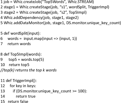
Figure 10: An example streaming job in Whiz

Appendix B Allocating Capsules to Machines ILP

Objectives (to be minimized):
$O_{1}$	$\max_{i}\left(\displaystyle\sum\limits_{k}(b^{k}_{i}+x^{k}_{i}e^{k})\right)$
$O_{2}$	$\displaystyle\sum\limits_{k}\left(P^{k}-\left(\displaystyle\sum\limits_{i\in I_{-}^{k}}x_{i}^{k}\right)b_{\hat{i}(k)}^{k}+\displaystyle\sum\limits_{i\in I_{+}^{k}}x_{i}^{k}\left(b_{i}^{k}+e^{k}\right)\right)$
$O_{3}$	$\displaystyle\sum\limits_{k}\left((1-f^{k})\displaystyle\sum\limits_{i\in I^{\circ}}x_{i}^{k}\right)$
Constraints:
$C_{1}$	$\displaystyle\sum\limits_{k:J(g_{k})=j}\left(b_{i}^{k}+x_{i}^{k}e^{k}\right)\leq Q_{j},\quad\forall j,i$
Variables:
$x_{i}^{k}$	Binary indicator denoting capsule $g_{k}$ is placed on machine $i$
Parameters:
$b_{i}^{k}$	Existing number of bytes of capsule $g_{k}$ in machine $i$
$e^{k}$	Expected number of remaining bytes for capsule, $g_{k}$
$P^{k}$	$e^{k}+\displaystyle\sum\limits_{i}b_{i}^{k}$
$J(g_{k})$	The job ID for job $g_{k}$
$\hat{i}(k)$	$\textrm{argmax}_{i}\quad b_{i}^{k}$
$I_{-}^{k},I_{+}^{k}$	$\{i:b_{i}^{k}\leq b_{\hat{i}(k)}^{k}-e^{k}\}$, $\{i:b_{i}^{k}>b_{\hat{i}(k)}^{k}-e^{k}\}$
$f^{k}$	Binary parameter indicating that capsules for same stage as $g_{k}$ share locations with capsules for preceding stages
$I^{\circ}$	Set of machines where capsules of preceding stages are stored
$Q_{j}$	Administrative storage quota for job, $j$.

Figure 11: Binary ILP formulation for capsule placement.

We consider how to place multiple jobs’ capsules to avoid hotspots, reduce per-capsule spread (for data locality) and minimize job runtime impact on data loss. We formulate a binary integer linear program (see Fig. 11) to this end. The indicator decision variables, $x_{i}^{k}$, denote that all future data to capsule $g_{k}$ is materialized at machine $M_{i}$. The ILP finds the best $x_{i}^{k}$’s that minimizes a multi-part weighted objective function, one part each for the three objectives mentioned above.

The first part ($O_{1}$) represents the maximum amount of data stored across all machines across all capsules. Minimizing this ensures load balance and avoids hotspots. The second part ($O_{2}$) represents the sum of data-spread penalty across all capsules. Here, for each capsule, we define the primary location as the machine with the largest volume of data for that capsule. The total volume of data in non-primary locations is the data-spread penalty, incurred from shuffling the data prior to processing it. The third part ($O_{3}$) is the sum of fault-tolerance penalties across capsules. Say a machine $m$ storing intermediate for current stage $s$ fails; then we have to re-execute $s$ to regenerate the data. If the machine also holds data for ancestor stages of $s$ then multiple stages have to be re-executed. If we ensure that data from parent and child stages are stored on different machines, then, upon child data failure only the child stage has to be executed. We model this by imposing a penalty whenever a capsule in the current stage is materialized on the same machine as the parent stage. Penalties $O_{2}$, $O_{3}$ need to be minimized.

Finally, we impose isolation constraint ($C_{1}$) requiring the total data for a job to not exceed an administrator set quota $Q_{j}$. Quotas help ensure isolation across jobs.

However, solving this ILP at scale can take several tens of seconds delaying capsule placement. Thus, Whiz uses a linear-time rule-based heuristic to place capsules (as described in §4).

Appendix C Whiz Microbenchmarks

Apart from the experiments on the 50-machine cluster (§9), we also ran several microbenchmarks to delve deeper into Whiz’s data-driven benefits. The microbenchmarks were run on a 5 machine cluster and the workloads consists of the following jobs: $\mathbb{J}_{1}$ ($v_{1}\rightarrow v_{2}$) and $\mathbb{J}_{2}$ ($v_{1}\rightarrow v_{2}\rightarrow v_{3}$). These patterns typically occur in TPC- DS queries.

Skew and parallelism: Fig. 12a shows the execution of one of the $\mathbb{J}_{2}$ queries from our workload when running Whiz and CC. Whiz improves JCT by $2.67\times$ over CC. CC decides stage parallelism tied to the number of data partitions. That means stage $v_{1}$ generates $2$ intermediate partitions as configured by the user and $2$ tasks of $v_{2}$ will process them. However, execution of $v_{1}$ leads to data skew among the $2$ partitions ($1GB$ and $4GB$).On the other hand, Whiz ends up generating capsules that are approximately equal in size and decides at runtime a max. input size per task of $1GB$ (twice the largest capsule). This leads to running $5$ tasks of $v_{2}$ with equal input size and $2.1\times$ faster completion time of $v_{2}$ than CC.

Over-parallelizing execution does not help. With CC, $v_{2}$ generates $12$ partitions processed by $12$ $v_{3}$ tasks. Under resource crunch, tasks get scheduled in multiple waves (at $570$s in Fig. 12a) and completion time for $v_{3}$ suffers ($85$s). In contrast, Whiz assigns at runtime only $5$ tasks of $v_{3}$ which can run in a single wave; $v_{3}$ finishes $1.23\times$ faster.

Straggler mitigation: We run an instance of $\mathbb{J}_{1}$ with $1$ task of $v_{1}$ and $1$ task of $v_{2}$ with an input size of $1GB$. A slowdown happens at the $v_{2}$ task, which was assigned 2 capsules by Whiz.

In CC (Fig. 12b), once a straggler is detected ($v_{2}$ task at $203$s), it is allowed to continue, and a speculative task $v^{\prime}_{2}$ is launched that duplicates $v_{2}$’s work. The work completes when $v_{2}$ or $v^{\prime}_{2}$ finishes (at $326$s). In Whiz, upon straggler detection, the straggler ($v_{2}$) is notified to finish processing the current capsule; a task $v^{\prime}_{2}$ is launched and assigned data from $v_{2}$’s unprocessed capsule. $v_{2}$ finishes processing the first capsule at $202$s; $v^{\prime}_{2}$ processes the other capsule and finishes $1.7\times$ faster than $v^{\prime}_{2}$ in CC.

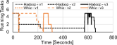
(a)

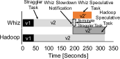
(b)

Figure 12: (a) Controlling task parallelism significantly improves Whiz’s performance over CC. (b) Straggler mitigation with Whiz and CC.

Runtime logic changes: We consider a job which processes words and, for words with $<100$ occurrences, sorts them by frequency. The program structure is $v_{1}\rightarrow v_{2}\rightarrow v_{3}$, where $v_{1}$ processes input words, $v_{2}$ computes word occurrences, and $v_{3}$ sorts the ones with $<100$ occurrences. In CC, $v_{1}$ generates $17GB$ of data organized in $17$ partitions; $v_{2}$ generates $8GB$ organized in $8$ partitions. Given this, $17$ $v_{2}$ tasks and $8$ $v_{3}$ tasks execute, leading to a CC JCT of $220$s. Here, the entire data generated by $v_{2}$ has to be analyzed by $v_{3}$. In contrast, Whiz registers a custom DS module to monitor #occurrences of all the words in the capsules generated by $v_{2}$. We implement actions to ignore $v_{2}$ capsules that don’t satisfy the processing criteria of $v_{3}$ (§6.3). At runtime, $2$ statistics events are triggered by the DS module, and $6$ tasks of $v_{3}$ (instead of $8$) are executed; JCT is $165$s ($1.4\times$ better).

References

- [1] Apache Giraph. http://giraph.apache.org.
- [2] Apache Hadoop. http://hadoop.apache.org.
- [3] Apache Hive. http://hive.apache.org.
- [4] Apache Samza. http://samza.apache.org.
- [5] Apache Tez. http://tez.apache.org.
- [6] Cloudlab. https://cloudlab.us.
- [7] Presto | Distributed SQL Query Engine for Big Data. prestodb.io.
- [8] Protocol Buffers. https://bit.ly/1mISy49.
- [9] Spark SQL. https://spark.apache.org/sql.
- [10] Storm: Distributed and fault-tolerant realtime computation. http://storm-project.net.
- [11] S. Agarwal, S. Kandula, N. Burno, M.-C. Wu, I. Stoica, and J. Zhou. Re-optimizing data parallel computing. In NSDI, 2012.
- [12] G. Ananthanarayanan, A. Ghodsi, S. Shenker, and I. Stoica. Effective Straggler Mitigation: Attack of the Clones. In NSDI, 2013.
- [13] G. Ananthanarayanan, S. Kandula, A. Greenberg, I. Stoica, Y. Lu, B. Saha, and E. Harris. Reining in the outliers in mapreduce clusters using Mantri. In OSDI, 2010.
- [14] M. Armbrust, R. S. Xin, C. Lian, Y. Huai, D. Liu, J. K. Bradley, X. Meng, T. Kaftan, M. J. Franklin, A. Ghodsi, and M. Zaharia. Spark SQL: Relational data processing in Spark. In SIGMOD, 2015.
- [15] L. Bindschaedler, J. Malicevic, N. Schiper, A. Goel, and W. Zwaenepoel. Rock you like a hurricane: Taming skew in large scale analytics. In EuroSys, 2018.
- [16] P. Boldi, M. Rosa, M. Santini, and S. Vigna. Layered label propagation: A multiresolution coordinate-free ordering for compressing social networks. In WWW, 2011.
- [17] P. Boldi and S. Vigna. The webgraph framework i: Compression techniques. In WWW, 2004.
- [18] P. Carbone, A. Katsifodimos, S. Ewen, V. Markl, S. Haridi, and K. Tzoumas. Apache flink: Stream and batch processing in a single engine. Bulletin of the IEEE Computer Society Technical Committee on Data Engineering, 36(4), 2015.
- [19] M. Chowdhury, M. Zaharia, J. Ma, M. I. Jordan, and I. Stoica. Managing data transfers in computer clusters with Orchestra. In SIGCOMM, 2011.
- [20] J. Dean and S. Ghemawat. MapReduce: Simplified data processing on large clusters. In OSDI, 2004.
- [21] A. Deshpande, Z. Ives, and V. Raman. Adaptive query processing. Found. Trends databases, 1(1):1–140, Jan. 2007.
- [22] A. Ghodsi, M. Zaharia, B. Hindman, A. Konwinski, S. Shenker, and I. Stoica. Dominant Resource Fairness: Fair allocation of multiple resource types. In NSDI, 2011.
- [23] J. E. Gonzalez, Y. Low, H. Gu, D. Bickson, and C. Guestrin. Powergraph: Distributed graph-parallel computation on natural graphs. In OSDI, 2012.
- [24] J. E. Gonzalez, R. S. Xin, A. Dave, D. Crankshaw, M. J. Franklin, and I. Stoica. GraphX: Graph processing in a distributed dataflow framework. In OSDI, 2014.
- [25] K. A. Hua and C. Lee. Handling data skew in multiprocessor database computers using partition tuning. In VLDB, 1991.
- [26] B. Huang, N. W. Jarrett, S. Babu, S. Mukherjee, and J. Yang. Cümülön: Matrix-based data analytics in the cloud with spot instances. PVLDB, 9(3):156–167, 2015.
- [27] B. Huang and J. Yang. Cümülön-d: data analytics in a dynamic spot market. PVLDB, 10(8):865–876, 2017.
- [28] P. Hunt, M. Konar, F. P. Junqueira, and B. Reed. Zookeeper: Wait-free coordination for internet-scale systems. In ATC, 2010.
- [29] E. Jonas, Q. Pu, S. Venkataraman, I. Stoice, and B. Recht. Occupy the cloud: Distributed computing for the 99%. In SOCC, 2017.
- [30] Q. Ke, M. Isard, and Y. Yu. Optimus: A dynamic rewriting framework for data-parallel execution plans. In EuroSys, 2013.
- [31] M. Kitsuregawa and Y. Ogawa. Bucket spreading parallel hash: A new, robust, parallel hash join method for data skew in the super database computer (sdc). In VLDB, 1990.
- [32] A. Klimovic, Y. Wang, P. Stuedi, A. Trivedi, J. Pfefferle, and C. Kozyrakis. Pocket: Elastic ephemeral storage for serverless analytics. In OSDI, 2018.
- [33] M. Kornacker, A. Behm, V. Bittorf, T. Bobrovytsky, C. Ching, A. Choi, J. Erickson, M. Grund, D. Hecht, M. Jacobs, I. Joshi, L. Kuff, D. Kumar, A. Leblang, N. Li, I. Pandis, H. Robinson, D. Rorke, S. Rus, J. Russell, D. Tsirogiannis, S. Wanderman-Milne, and M. Yoder. Impala: A modern, open-source SQL engine for Hadoop. In CIDR, 2015.
- [34] S. Kulkarni, N. Bhagat, M. Fu, V. Kedigehalli, C. Kellogg, S. Mittal, J. M. Patel, K. Ramasamy, and S. Taneja. Twitter heron: Stream processing at scale. In SIGMOD, 2015.
- [35] Y. Kwon, M. Balazinska, B. Howe, and J. Rolia. Skewtune: Mitigating skew in mapreduce applications. In SIGMOD, 2012.
- [36] W. Lin, Z. Qian, J. Xu, S. Yang, J. Zhou, and L. Zhou. Streamscope: continuous reliable distributed processing of big data streams. In NSDI, 2016.
- [37] K. Mahajan, M. Chowdhury, A. Akella, and S. Chawla. Dynamic query re-planning using QOOP. In OSDI, 2018.
- [38] G. Malewicz, M. H. Austern, A. J. Bik, J. C. Dehnert, I. Horn, N. Leiser, and G. Czajkowski. Pregel: A system for large-scale graph processing. In SIGMOD, 2010.
- [39] X. Meng, J. K. Bradley, B. Yavuz, E. R. Sparks, S. Venkataraman, D. Liu, J. Freeman, D. B. Tsai, M. Amde, S. Owen, D. Xin, R. Xin, M. J. Franklin, R. Zadeh, M. Zaharia, and A. Talwalkar. MLlib: Machine learning in Apache Spark. CoRR, abs/1505.06807, 2015.
- [40] D. G. Murray, F. McSherry, R. Isaacs, M. Isard, P. Barham, and M. Abadi. Naiad: A timely dataflow system. In SOSP, 2013.
- [41] D. G. Murray, M. Schwarzkopf, C. Smowton, S. Smith, A. Madhavapeddy, and S. Hand. Ciel: A Universal Execution Engine for Distributed Data-Flow Computing. In NSDI, 2011.
- [42] Q. Pu, S. Venkataraman, and I. Stoica. Shuffling, fast and slow: Scalable analytics on serverless infrastructure. In NSDI, 2019.
- [43] B. Saha, H. Shah, S. Seth, G. Vijayaraghavan, A. Murthy, and C. Curino. Apache tez: A unifying framework for modeling and building data processing applications. In SIGMOD, 2015.
- [44] P. Snyder. tmpfs: A virtual memory file system. In European UNIX Users’ Group Conference, 1990.
- [45] A. Thusoo, R. Murthy, J. S. Sarma, Z. Shao, N. Jain, P. Chakka, S. Anthony, H. Liu, and N. Zhang. Hive – a petabyte scale data warehouse using Hadoop. In ICDE, 2010.
- [46] A. Toshniwal, S. Taneja, A. Shukla, K. Ramasamy, J. M. Patel, S. Kulkarni, J. Jackson, K. Gade, M. Fu, J. Donham, N. Bhagat, S. Mittal, and D. Ryaboy. Storm@twitter. In SIGMOD, 2014.
- [47] V. K. Vavilapalli, A. C. Murthy, C. Douglas, S. Agarwal, M. Konar, R. Evans, T. Graves, J. Lowe, H. Shah, S. Seth, B. Saha, C. Curino, O. O’Malley, S. Radia, B. Reed, and E. Baldeschwieler. Apache Hadoop YARN: Yet another resource negotiator. In SoCC, 2013.
- [48] L. Wei, Q. Zhengping, X. Junwei, Y. Sen, Z. Jingren, and Z. Lidong. Streamscope: Continuous reliable distributed processing of big data streams. In NSDI, 2016.
- [49] R. S. Xin, J. Rosen, M. Zaharia, M. J. Franklin, S. Shenker, and I. Stoica. Shark: SQL and rich analytics at scale. In SIGMOD, 2013.
- [50] Y. Xu, P. Kostamaa, X. Zhou, and L. Chen. Handling data skew in parallel joins in shared-nothing systems. In SIGMOD, 2008.
- [51] M. Zaharia, D. Borthakur, J. Sen Sarma, K. Elmeleegy, S. Shenker, and I. Stoica. Delay scheduling: A simple technique for achieving locality and fairness in cluster scheduling. In EuroSys, 2010.
- [52] M. Zaharia, M. Chowdhury, T. Das, A. Dave, J. Ma, M. McCauley, M. Franklin, S. Shenker, and I. Stoica. Resilient Distributed Datasets: A fault-tolerant abstraction for in-memory cluster computing. In NSDI, 2012.
- [53] M. Zaharia, T. Das, H. Li, S. Shenker, and I. Stoica. Discretized streams: Fault-tolerant stream computation at scale. In SOSP, 2013.
- [54] M. Zaharia, A. Konwinski, A. D. Joseph, R. Katz, and I. Stoica. Improving MapReduce performance in heterogeneous environments. In OSDI, 2008.