The distribution of first hitting times of random walks on directed Erdős-Rényi networks

Abstract

We present analytical results for the distribution of first hitting times of random walkers (RWs) on directed Erdős-Rényi (ER) networks. Starting from a random initial node, a random walker hops randomly along directed edges between adjacent nodes in the network. The path terminates either by the retracing scenario, when the walker enters a node which it has already visited before, or by the trapping scenario, when it becomes trapped in a dead-end node from which it cannot exit. The path length, namely the number of steps, $d$, pursued by the random walker from the initial node up to its termination, is called the first hitting time. Using recursion equations, we obtain analytical results for the tail distribution of first hitting times, $P(d>\ell)$. The results are found to be in excellent agreement with numerical simulations. It turns out that the distribution $P(d>\ell)$ can be expressed as a product of an exponential distribution and a Rayleigh distribution. We obtain expressions for the mean, median and standard deviation of this distribution in terms of the network size and its mean degree. We also calculate the distribution of last hitting times, namely the path lengths of self-avoiding walks on directed ER networks, which do not retrace their paths. The last hitting times are found to be much longer than the first hitting times. The results are compared to those obtained for undirected ER networks. It is found that the first hitting times of RWs in a directed ER network are much longer than in the corresponding undirected network. This is due to the fact that RWs on directed networks do not exhibit the backtracking scenario, which is a dominant termination mechanism of RWs on undirected networks. It is shown that our approach also applies to a broader class of networks, referred to as semi-ER networks, in which the distribution of in-degrees is Poisson, while the out-degrees may follow any desired distribution with the same mean as the in-degree distribution.

, ,

1 Introduction

Random walk (RW) models provide a framework for the study of diffusion and other stochastic processes [1, 2]. These models were studied extensively on regular lattices and random networks. An RW can be considered as a particle which resides on the sites of the lattice or network, such that at each time step it hops randomly to one of the neighbors of its current site. Random walks on lattices provide a discrete spatio-temporal description of diffusion processes in the Euclidean space. In the large-scale and long-time limit, the evolution of the spatial probability distribution of an RW can be described by the diffusion equation, while at small scales, the discreteness of the lattice plays an important role. Unlike a ballistic particle which moves in a fixed direction at a constant speed, an RW picks a random direction at each time step. As a result, the mean distance reached by an RW from its initial location scales like $t^{1/2}$, compared to $t$ for a ballistic particle, where $t$ is the elapsed time. More precisely, the probability distribution of an RW starting at the origin of a regular lattice in $D$ dimensions follows a Gaussian distribution, whose standard deviation scales like $t^{1/2}$, for any finite dimension, $D$. RWs maintain no memory in the sense that the probability distribution of the next move depends only on the current state of the system. Therefore, they satisfy the Markovian condition and can be studied using the methodologies developed for Markovian processes [3]. RW problems are commonly posed as initial value problems, in which the initial conditions are specified and the task is to calculate the spatial probability distribution at a later time. However, in an alternative setting called first passage problems, one is interested in questions like how long it will take for the RW to reach a given location for the first time [4]. The general problem is to calculate the distribution of first passage times for the given setting, or properties of the distribution such as the mean first passage time. An RW on a lattice hops randomly at each time step to one of the nearest neighbors of its current site. In some of the steps it hops into new sites which have not been visited before. In other steps it hops into previously visited sites. The mean number of distinct sites, $s(t)$, visited up to time $t$ is thus smaller than $t$. It was shown that in one dimension $s(t)\sim t^{1/2}$, in two dimensions $s(t)\sim t/\ln t$, while in three and more dimensions $s(t)\sim t$ [5]. It was recently shown that on ER networks, the number of distinct nodes visited up to time $t$ scales linearly with $t$ [6], resembling the results obtained for RWs on high dimensional lattices. On finite networks other interesting quantities emerge, such as the mean first passage time between a random pair of nodes [7] and the mean cover time, namely the average number of steps required for the RW to visit all the nodes in the network [8].

An important time scale which appears in random walks on networks is the first hitting time, also referred to as the first intersection length [9, 10, 11, 12]. This time scale emerges in a class of RW models in which the RW keeps hopping until it enters a node which it has already visited before or becomes trapped in a node from which it cannot exit. At this point the path is terminated, as is the case in a large class of processes called first passage problems [4]. The resulting path length, namely the number of time steps up to its termination, is called the first hitting time. In Ref. [13] we presented analytical results for the distribution of first hitting times of RWs on undirected Erdős-Rényi (ER) networks [14, 15, 16]. On undirected networks, the RW path may terminate either by backtracking into the previous node or by retracing itself, namely stepping into a node which was already visited two or more time steps earlier. By calculating the probabilities of these two scenarios, we obtained analytical results for the distribution of first hitting times of RWs on ER networks. Another interesting time scale is the last hitting time [10] of a self avoiding walk (SAW) [17, 18], which does not retrace its path but may be trapped once it enters a node which does not have any yet unvisited neighbors. In Ref. [19] we presented analytical results for the distribution of last hitting times of SAWs on undirected ER networks.

Most of the networks encountered in physical, chemical, biological, technological and social systems are directed networks. Therefore, it is important to study diffusive processes on directed networks and the RW is the simplest dynamical model describing such processes. The dynamical properties of RWs on directed networks are different from those of RWs on undirected networks. In undirected networks each RW path between node $i$ and node $j$ may be pursued in both directions. In directed networks some pairs of nodes may be connected only in one direction and not in the other direction. Even if nodes $i$ and $j$ are connected in both directions, the paths in opposite directions are not the same. While undirected networks exhibit a single degree distribution, $p(k)$, directed networks exhibit two distinct degree distributions, namely the distribution of in-degrees, $p^{\rm in}(k)$, and the distribution of out-degrees, $p^{\rm out}(k)$. The two distributions must have the same mean, namely $\langle k\rangle^{\rm in}=\langle k\rangle^{\rm out}$. While in undirected networks the frequency in which an RW visits a node, $i$, is simply proportional to its degree, $k_{i}$, in directed networks such visit frequencies depend not only on the in-degree $k_{i}^{\rm in}$ but on the overall structure of the surrounding network. Finally, directed networks exhibit dead-end nodes which have incoming links but no outgoing links. As a result, RWs which enter such nodes becomes trapped.

In this paper we present analytical results for the distribution of first hitting times of RWs on directed ER networks [20, 21, 22]. In these networks each pair of nodes, $i$ and $j$, are connected, with probability $p$ by a directed link from $i$ to $j$, and independently, with the same probability, by a directed link from $j$ to $i$. We also calculate the mean, median and standard deviation of the distribution of first hitting times. The results are found to be in excellent agreement with numerical simulations. Unlike the case of undirected networks in which backtracking moves are always possible, on directed networks backtracking may occur only when the current node and the previous node are connected in both directions. Moreover, on a directed network an RW may become trapped in a dead-end node which does not have any outgoing links. As a result, an RW path on a directed ER network may terminate either by trapping or by retracing its path. We obtain analytical results for the overall probabilities, $p_{\rm trap}$ and $p_{\rm ret}$, that an RW starting from a random node will terminate by trapping or by retracing, respectively. It is found that in dilute networks most paths terminate by trapping while in dense networks most paths terminate by retracing. We obtain expressions for the conditional probabilities, $P(d>\ell|{\rm trap})$ and $P(d>\ell|{\rm ret})$, of RWs which terminate by trapping or by retracing, respectively, as well for the conditional probabilities $P({\rm trap}|d>\ell)$ and $P({\rm ret}|d>\ell)$. It is found that the probability of termination by trapping decreases with the path length while the probability of termination by retracing increases with the path length. Since most of the directed networks in nature exhibit different distributions of in-degrees and out-degrees, it is of interest to disentangle the effect of these distributions on the distribution of first hitting times. To this end, we extend our studies to a broader class of directed networks, referred to as semi-ER networks, in which the in-degree distribution is Poisson and the out-degrees follow any desired distribution with the same mean as the in-degree distribution. We present analytical results for the distribution of first hitting times in such networks. We also consider the distribution of last hitting times on directed ER networks.

The paper is organized as follows. In Sec. 2 we present relevant properties of directed ER networks. In Sec. 3 we describe the random walk model on directed ER networks. In Sec. 4 we consider the evolution of the subnetwork of the yet-unvisited nodes. In Sec. 5 we present analytical results the distribution of last hitting times of RWs on directed ER networks. In Sec. 6 we present analytical results for the distribution of first hitting times of RWs on directed ER networks. In Sec. 7 we obtain analytical expressions for two central measures (mean and median) and for a dispersion measure (the standard deviation) of this distribution. In Sec. 8 we calculate the distributions of path lengths conditioned on the termination mechanism. In Sec. 9 we generalize the analysis to directed semi-ER networks, which exhibit a Poisson in-degree distribution and any desired out-degree distribution. The results are summarized and discussed in Sec. 10. In Appendix A we present the detailed calculation of the contribution of the retracing mechanism to the distribution of first hitting times.

2 The directed Erdős-Rényi network

The directed ER network is the simplest model of a directed random network. It consists of $N$ nodes such that a directed edge, or link, from any node, $i$, to any other node, $j$, exists with probability $p$, independently of the existence of the opposite link, or any other link. Therefore, the probability that a random pair of nodes, $i$ and $j$ are connected in both directions is $p^{2}$. In directed networks each node, $i$ has an in-degree, $k_{i}^{in}$, which is the number of incoming links and an out-degree, $k_{i}^{out}$, which is the number of outgoing links. In general one should distinguish between the degree distribution of incoming links, $p^{\rm in}(k)$, and the degree distribution of outgoing links, $p^{\rm out}(k)$ [23]. Since each link is directed out of one node and into another node, the mean, $\langle k\rangle^{\rm in}$, of $p^{\rm in}(k)$ must be equal to the mean, $\langle k\rangle^{\rm out}$, of $p^{\rm out}(k)$.

In directed ER networks, both distributions, $p^{\rm in}(k)$ and $p^{\rm out}(k)$, are binomial distributions. Therefore, in the sparse limit ($p\ll 1$) they are approximated by a Poisson distribution of the form [20]

$$p^{\rm in}(k)=p^{\rm out}(k)=p(k)=\frac{{c}^{k}}{k!}e^{-c},$$ (1)

where the mean in-degree and the mean out-degree are given by $c=(N-1)p$. It is important to note that the in-degree and out-degree of each node are uncorrelated. Also, there are no degree-degree correlations between adjacent nodes. The adjacency matrix, $A$, of a directed ER network of $N$ nodes is a random $N\times N$ matrix with a zero diagonal and whose off-diagonal entries are $1$ with probability $p$ and $0$ with probability $1-p$. Note that unlike the undirected case, $A$ is not necessarily a symmetric matrix.

The percolation properties of directed ER networks differ from those of their undirected counterparts [23, 24, 25]. Undirected ER networks exhibit a percolation transition at $c=1$, above which the network consists of a giant cluster, small, isolated components and isolated nodes. On the giant cluster, every node can be reached from any other node. The percolation transition of a directed ER network also takes place at $c=1$, above which a giant cluster is formed. However, due to the directionality of the links, not all pairs of nodes on the giant cluster can be reached from each other along paths which consist of directed links. The subgraph of the giant cluster in which each pair of nodes can be reached from each other in both directions is called the giant strongly connected component (GSCC) [23, 24, 25]. The set of nodes on the giant cluster which can be reached from the GSCC is called the out component, while the set of nodes from which the GSCC can be reached is called the in component. In addition, there are some nodes on the giant cluster which do not belong either to the in component or to the out component. These nodes are referred to as tendrils [23]. The probability of a random node in a directed ER network to be an isolated node is $\exp(-2c)$. Also, the probability of a random node to have only incoming links or only outgoing links is $\exp(-c)$. A node which has only outgoing links cannot be reached unless it is the initial node in the RW path. When the RW enters a node which has only incoming links, it becomes trapped and the RW path terminates.

3 The random walk model

Consider an RW on a directed random network of $N$ nodes. Each time step the walker chooses randomly one of the outgoing edges of the current node, and hops along this edge to an adjacent node. The RW path terminates when it steps into a node which it has already visited before (retracing scenario) or when it enters a dead-end node which has only incoming links (trapping scenario). The initial node is chosen randomly among the nodes for which the out-degree satisfies $k_{i}^{\rm out}\geq 1$, so the RW is guaranteed to make at least one move. The resulting path length, $d$, namely the number of steps pursued by the RW until its termination, is referred to as the first hitting time. In the analysis below we do not include the termination step itself as a part of the RW path. This means that the path length of an RW which pursued $\ell$ steps and terminated at the $\ell+1$ step is $d=\ell$. The path includes $d+1$ nodes, since the initial node is also counted as a part of the path.

4 Evolution of the subnetwork of the yet-unvisited nodes

Consider an RW starting from a random node on a directed ER network. The RW divides the network into two subnetworks: one consists of the already visited nodes and the other consists of the yet-unvisited nodes. After $t$ time steps the size of the subnetwork of visited nodes is $t+1$ (including the initial node), while the size of the network of yet unvisited nodes is $N(t)=N-t-1$. Here we focus on the subnetwork of the yet-unvisited nodes. Its in-degree distribution and out-degree distribution evolve in time. We denote these distributions, at time $t$, by $p^{\rm in}_{t}(k)$, and $p^{\rm out}_{t}(k)$, $k=0,\dots,N(t)-1$, respectively, where $p^{\rm in}_{0}(k)=p^{\rm out}_{0}(k)=p(k)$, which is given by Eq. (1). The mean in and out degrees of this subnetwork, which are given by

$$\langle k\rangle^{\rm in}_{t}=\sum_{k=0}^{N(t)-1}kp^{\rm in}_{t}(k),$$ (2)

and

$$\langle k\rangle^{\rm out}_{t}=\sum_{k=0}^{N(t)-1}kp^{\rm out}_{t}(k),$$ (3)

evolve accordingly. Since the number of incoming links is equal to the number of outgoing links, the mean degrees of the two distributions must satisfy $\langle k\rangle^{\rm in}_{t}=\langle k\rangle^{\rm out}_{t}$, and are denoted by $c(t)$.

We now examine the evolution of the subnetwork of the yet-unvisited nodes in terms of the mean numbers of incoming and outgoing links which are removed at each step. Deleting a node along the RW path removes, on average, $c(t)$ incoming links and $c(t)$ outgoing links from the node itself as well as $c(t)$ incoming links and $c(t)$ outgoing links from its neighbors, which remain on the subnetwork of the yet-unvisited nodes. Denoting the initial in-degree and out-degree of node $i$, by $k^{\rm in}_{i}$ and $k^{\rm out}_{i}$, respectively we note that $\sum_{i=1}^{N}k^{\rm in}_{i}=\sum_{i=1}^{N}k^{\rm out}_{i}=Nc$. Thus, the time dependence of the mean degree can be expressed by

$$c(t)=\frac{Nc-2\sum_{t^{\prime}=0}^{t-1}c(t^{\prime})}{N-t}.$$ (4)

This implies that $c(t)$ obeys the recursion equation

$$c(t)=\left(1-\frac{1}{N-t}\right)c(t-1),$$ (5)

in which the coefficient on the right hand side depends on $t$. This equation is solved by

$$c(t)=\left(1-\frac{t}{N-1}\right)c.$$ (6)

For RWs on directed random networks, there is a higher probability for the walker to enter nodes with high incoming degrees. More precisely, the probability that in the next time step the RW will step into a node of in-degree $k$ is $kp^{\rm in}(k)/c$. However, by the time the RW enters the next node, the previous node is effectively deleted, together with the edge connecting the two nodes. Therefore, when the walker enters a node of in-degree $k$, the in-degree of this node is reduced to $k-1$. A special property of the Poisson distribution is that $kp(k)/c=p(k-1)$. This means that the probability that the node visited at time $t+1$ will be of degree $k$ is given by $p_{t}(k-1)$. The outcome of this reasoning is that the probability of the RW to visit a node of in-degree $k$ in the smaller network at time $t$ is simply $p^{\rm in}_{t}(k)$, as if it makes a random choice of a node in the smaller network. The result of this exact, yet delicate, balance is that the subnetwork of the yet-unvisited nodes at time $t$, is a directed ER network with mean in and out degrees equal to $c(t)$, as well as degree distributions, $p_{t}^{\rm in}(k)$ and $p_{t}^{\rm out}(k)$, given by

$$p_{t}(k)=\frac{c(t)^{k}}{k!}e^{-c(t)}.$$ (7)

It is interesting to note that a similar result is also obtained for undirected ER networks [19].

5 The distribution of last hitting times

The paths pursued by the RWs studied here are, in fact, segments of SAW paths. In case of termination by trapping the RW path is identical to an SAW path, while in case of termination by retracing the RW path consists of the initial segment of a longer SAW path. Therefore, the distribution of first hitting times is bounded from above by the distribution of path lengths of SAWs on the same networks, also referred to as the last hitting times. Below we present analytical results for the distribution of last hitting times. Consider an SAW on an ER network, which starts from a random node, $i$, with an out-degree $k^{\rm out}_{i}\geq 1$. The SAW hops through directed links between adjacent nodes until it reaches a node from which it cannot exit. At that stage the path terminates. The out-degree of node $i$ in the subnetwork of the yet-unvisited nodes, at time $t$, is given by $k_{i}^{\rm out}(t)$. The termination of an SAW path occurs when it enters a node for which $k_{i}^{\rm out}(t)=0$. The probability that a random node does not have outgoing links in the subnetwork of the yet-unvisited nodes at time $t$ is $p_{t}^{\rm out}(k=0)$. The conditional probability that the SAW will proceed from time $t$ to time $t+1$ without being trapped is denoted by $P(d>t|d>t-1)$, where $d$ represents the random variable of the path length and $t$ represents its actual value. This conditional probability is given by $P(d>t|d>t-1)=1-p_{t}^{\rm out}(k=0)$. Thus, the probability that the path length of the SAW will be longer than $\ell$, also known as the tail distribution, is given by

$$P(d>\ell)=P(d>0)\prod_{t=1}^{\ell}P(d>t|d>t-1).$$ (8)

The probability $P(d>0)=1$ since the initial node is chosen randomly among the nodes for which $k_{i}^{\rm out}\geq 1$. Thus, the tail distribution takes the form

$$P(d>\ell)=\prod_{t=1}^{\ell}\left[1-p_{t}^{\rm out}(k=0)\right].$$ (9)

While Eq. (9) applies to any network, in the case of a directed ER network there is an explicit expression for the probability of a node to have no outgoing links at time $t$, of the form $p_{t}^{\rm out}(k=0)=\exp[-c(t)]$. Therefore, the tail distribution takes the form

$$P(d>\ell)=\prod_{t=1}^{\ell}\left[1-e^{-c(t)}\right].$$ (10)

To obtain a closed form expression for the tail distribution, $P(d>\ell)$, we take the natural logarithm on both sides of Eq. (10). This leads to

$$\ln\left[P\left(d>\ell\right)\right]=\sum_{t=1}^{\ell}\ln\left[1-\exp\left(\frac{ct}{N-1}-c\right)\right].$$ (11)

Replacing this sum by an integral we obtain

$$\ln\left[P\left(d>\ell\right)\right]=\int_{1/2}^{\ell+1/2}\ln\left[1-\exp\left(\frac{ct}{N-1}-c\right)\right]dt,$$ (12)

where the limits of the integration are set such that the summation over each integer, $i$, is replaced by an integral over the range $(i-1/2,i+1/2)$. This integral is in fact a partial Bose-Einstein integral, which can be expressed in terms of the Polylogarithm ${\rm Li}_{n}(x)$ function [26]

$$P(d>\ell)=\exp\left\{\frac{N-1}{c}\left[{\rm Li}_{2}\left(e^{-\left(1-\frac{1}{2(N-1)}\right)c}\right)-{\rm Li}_{2}\left(e^{-\left(1-\frac{\ell+1/2}{N-1}\right)c}\right)\right]\right\}.$$ (13)

In approximating the sum of Eq. (11) by the integral of Eq. (12) we have used the formulation of the middle Riemann sum. Since the function $\ln[P(d>\ell)]$ is a monotonically decreasing function, the value of the integral is over-estimated by the left Riemann sum, $L(\ell)$, and under-estimated by the right Riemann sum, $R(\ell)$. The error involved in this approximation is thus bounded by the difference $\Delta(\ell)=L(\ell)-R(\ell)$, which satisfies $\Delta(\ell)=\ln(e^{c}-1)-\ln[e^{c}-e^{c(\ell+1)/(N-1)}]$. Thus, the relative error in $P(d>\ell)$ due to the approximation of the sum by an integral is bounded by $\eta_{\rm SI}\sim\ell/N$. Comparing the values obtained from the sum and the integral over a broad range of parameters, we find that the pre-factor of the error is very small, so in practice the error introduced by approximation of the sum by an integral is negligible.

For large networks ($N\gg 1$) one can further approximate the ${\rm Li}_{2}(x)$ function in Eq. (13) by the leading term in its Taylor expansion of the form ${\rm Li}_{2}(x)=\sum_{k=1}^{\infty}x^{k}/k^{2}$. We obtain

$$P\left(d>\ell\right)\simeq\exp\left[-\frac{N}{c}e^{-c}\left(e^{\frac{c}{N}\ell}-1\right)\right].$$ (14)

Evaluating the second order term we find that the relative error involved in this approximation is $\eta_{TE}\sim\ell/e^{2c}$. The expression for the tail distribution of last hitting times for directed ER networks, presented in Eq. (14) coincides with the Gompertz distribution [27, 28, 29, 30] of a random variable $X$, which takes the form

$$P(X>x)=\exp\left[-\eta\left(e^{ax}-1\right)\right]$$ (15)

for $x\geq 0$, with the scale parameter $a={c}/{N}$ and the shape parameter $\eta={N}e^{-c}/c$.

6 The distribution of first hitting times

An RW on a directed network hops randomly along directed edges until it steps into a previously visited node (retracing) or gets trapped in a node which does not have any outgoing edges (trapping). Unlike the case of an undirected network, a directed edge from the current node to the previous node exists only with probability $p$. Therefore, on a directed network the probability of a ’backtracking’ move of the RW from the current node to the previous node is the same as the probability to hop into any other node. As a result, on a directed network one does not need to treat the backtracking step as a special termination scenario which is different from the retracing scenario. The RW path on a directed network may terminate by retracing starting from the second time step, by hopping back into the initial node (in case that such a backward link exists, which occurs with probability $p$). However, as the termination move is not counted, the resulting path length is $\ell=1$. Since the initial node is chosen among the nodes which have at least one outgoing edge, termination by trapping cannot occur in the first step, justifying the statement that it may occur starting only from the second time step.

We denote the conditional probability that the RW path exceeds $t$ steps, given that it exceeds $t-1$ steps, by $P(d>t|d>t-1)$. It can be expressed in the form

$$P(d>t|d>t-1)=P_{\rm ret}(d>t|d>t-1)P_{\rm trap}(d>t|d>t-1),$$ (16)

where $P_{\rm trap}(d>t|d>t-1)$ is the probability that the RW path will not terminate by trapping at the $t+1$ time step, while $P_{\rm ret}(d>t|d>t-1)$ is the probability that it will not terminate by retracing, given that it has not terminated by trapping.

The probability that an RW will not terminate by trapping in the $t+1$ time step is given by the probability that the node it entered at time $t$ has an out-degree $k_{out}>0$ in the entire network (namely counting all its outgoing links regardless of whether they point towards nodes which were already visited or yet unvisited). This probability is given by

$$P_{\rm trap}(d>t|d>t-1)=\sum_{k=1}^{N-1}p^{\rm out}(k)=1-p^{\rm out}(0).$$ (17)

Inserting in Eq. (17) the Poisson distribution of Eq. (1) we obtain

$$P_{\rm trap}(d>t|d>t-1)=1-e^{-c}.$$ (18)

Note that this probability does not depend on the time, $t$.

Given that the RW has not terminated by trapping at the $t+1$ time step, the out-degree of the current node at time $t$ is conditioned to be $k^{\rm out}>0$. We will now evaluate the probability, $P_{\rm ret}(d>t|d>t-1)$, that the RW will also not terminate by retracing. This probability is given by $P_{\rm ret}(d>t|d>t-1)=\langle k^{\rm out}(t)|k^{\rm out}>0\rangle/\langle k^{\rm out}|k^{\rm out}>0\rangle$, where $k^{\rm out}(t)$ is the out-degree of the current node within the sub-network of the yet-unvisited nodes. Putting aside for a moment the condition $k^{\rm out}>0$, there are $N-1$ nodes in the network which may receive an outgoing link from the current node, each one of them with probability $p$. Thus, the expectation value of the number of outgoing links from the current node to its neighbors, through which the RW may hop at the $t+1$ time step, is $c=(N-1)p$. Since the number of yet unvisited nodes is $N-t-1$, we conclude that the current node is expected to have $c(t)=(N-t-1)p$ neighbors which have not yet been visited. In presence of the condition $k^{\rm out}>0$, we find that $\langle k^{\rm out}(t)|k^{\rm out}>0\rangle=c(t)/(1-e^{-c})$ and $\langle k^{\rm out}|k^{\rm out}>0\rangle=c/(1-e^{-c})$. We thus obtain

$$P_{\rm ret}(d>t|d>t-1)=\frac{c(t)}{c}.$$ (19)

Combining the results presented above, it is found that the probability that the path of the RW will not terminate at the $t+1$ time step is given by the conditional probability

$$P(d>t|d>t-1)=\frac{c(t)}{c}\left(1-e^{-c}\right).$$ (20)

In Fig. 1 we present the conditional probability $P(d>t|d>t-1)$ of first hitting times vs. $t$ for an RW on a directed ER network of size $N=1000$ and three values of $c$. The analytical results (solid lines) obtained from Eq. (20) are found to be in very good agreement with the numerical simulations (symbols), confirming the validity of this equation. Note that the numerical results become more noisy as $t$ increases, due to diminishing statistics, and eventually terminate. This is particularly apparent for the smaller values of $c$.

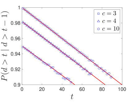
Figure 1: The conditional probability of first hitting times, $P(d>t|d>t-1)$ vs. $t$, obtained from Eq. (20) (solid lines) and from numerical simulations of RWs (symbols) on directed ER networks of size $N=1000$ and mean degrees $c=3$, $4$ and $10$ (squares, triangles and circles, respectively). The analytical and numerical results are found to be in very good agreement.

The tail distribution, $P(d>\ell)$, namely the probability that the path length of the RW will be longer than $\ell$ is given by

$$P(d>\ell)=P(d>0)\prod_{t=1}^{\ell}P(d>t|d>t-1).$$ (21)

The probability $P(d>0)=1$, since the initial node is chosen among the nodes with out-degrees $k_{\rm out}\geq 1$. The probability $P(d>\ell)$ can be written as a product of the form

$$P(d>\ell)=P_{\rm ret}(d>\ell)P_{\rm trap}(d>\ell),$$ (22)

where

$$P_{\rm trap}(d>\ell)=\prod_{t=1}^{\ell}\left(1-e^{-c}\right),$$ (23)

and

$$P_{\rm ret}(d>\ell)=\prod_{t=1}^{\ell}\frac{c(t)}{c}.$$ (24)

To obtain a closed form expression for the tail distribution, we take the natural logarithm on both sides of Eq. (22). This leads to

$$\ln\left[P\left(d>\ell\right)\right]=\ln\left[P_{\rm ret}\left(d>\ell\right)\right]+\ln\left[P_{\rm trap}\left(d>\ell\right)\right].$$ (25)

The calculation of $P_{\rm trap}(d>\ell)$ is simplified by the fact that $P_{\rm trap}(d>t|d>t-1)$ does not depend on $t$. As a result, Eq. (23) can be written in the form

$$P_{\rm trap}(d>\ell)=\left(1-e^{-c}\right)^{\ell}.$$ (26)

The termination by the trapping scenario can thus be considered as a Poisson process, in which the termination probability is fixed and depends only on the mean degree of the network. Taking the logarithm on both sides of Eq. (26) we obtain

$$\ln\left[P_{\rm trap}\left(d>\ell\right)\right]=\ell\ln\left(1-e^{-c}\right).$$ (27)

The detailed evaluation of $P_{\rm ret}(d>\ell)$ is presented in Appendix A, where $\ln P_{\rm ret}(d>\ell)$ is expressed as a sum, the sum is replaced by an integral and the integration is performed. Combining the results for $P_{\rm ret}\left(d>\ell\right)$ and $P_{\rm trap}\left(d>\ell\right)$ we obtain the tail distribution

$$P\left(d>\ell\right)\simeq\exp\left[\left(\ell+\frac{3}{2}-N\right)\ln\left(1-\frac{\ell+1/2}{N-1}\right)-\ell+\ell\ln\left(1-e^{-c}\right)-\frac{1}{2}\right].$$ (28)

Assuming that the RW paths are short compared to the network size, namely that $\ell\ll N$, one can use the approximation

$$\ln\left(1-\frac{\ell+1/2}{N-1}\right)\simeq-\frac{\ell+1/2}{N-1}-\frac{(\ell+1/2)^{2}}{2(N-1)^{2}},$$ (29)

which yields

$$P\left(d>\ell\right)\simeq\exp\left[-\frac{(\ell+1/2)^{2}}{2N}+\ell\ln\left(1-{e^{-c}}\right)\right].$$ (30)

Thus, the tail distribution of first hitting times of RWs on directed ER networks takes the form

$$P\left(d>\ell\right)\simeq\exp\left[-\left(\frac{\ell}{2\alpha}\right)^{2}-\beta\ell\right]$$ (31)

where

$$\alpha=\sqrt{\frac{N}{2}}$$ (32)

and

$$\beta=-\ln(1-e^{-c})+\frac{1}{4\alpha^{2}}.$$ (33)

The right hand side of Eq. (31) is, in fact, a product of a discrete Rayleigh distribution [26] and a discrete exponential distribution. The Rayleigh distribution accounts for the retracing scenario while the exponential distribution accounts for the trapping scenario.

Considering the next order in the series expansion of Eq. (29), we find that the relative error in Eq. (31), for $P(d>\ell)$, due to the truncation of the Taylor expansion after the second order is $\eta_{\rm TE}\sim\ell^{3}/N^{2}$. This error is very small as long as $\ell\ll N^{1/2}$. Note that paths of length $\ell\simeq N^{1/2}$, for which the error in $P(d>\ell)$ is noticeable, become prevalent only in the limit of dense networks, where $c>N^{1/2}$.

In Fig. 2 we present the tail distributions (top row) of first hitting times, $P(d>\ell)$, of RWs on directed ER networks of size $N=1000$ and $c=3$, $4$ and $10$. The theoretical results (solid lines), obtained from Eq. (28), are in excellent agreement with the results obtained from numerical simulations (circles). This agreement indicates that the approximation used in the analytical derivation, namely the replacement of a sum by an integral, is justified. The corresponding probability density functions,

$$P(d=\ell)=P(d>\ell-1)-P(d>\ell),$$ (34)

are shown in the bottom row. It is found that for small values of $c$ most paths are short and the probability density function is a monotonically decreasing function of $\ell$. As $c$ is increased, the distribution $P(d=\ell)$ shifts to the right and develops a well defined peak.

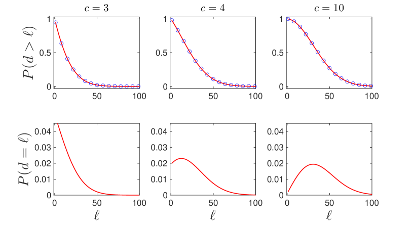
Figure 2: The tail distributions (top row) of first hitting times, $P(d>\ell)$ vs. $\ell$, of RWs on directed ER networks of size $N=1000$ and $c=3$, $4$ and $10$. The theoretical results, obtained from Eq. (28) (solid lines) are in excellent agreement with the results obtained from numerical simulations (circles). The corresponding probability distribution functions, $P(d=\ell)$, obtained from Eq. (34), are shown in the bottom row. The agreement with the numerical results is already established in the top row and therefore the numerical data is not shown in the bottom row.

7 Central and dispersion measures

In order to characterize the distribution of first hitting times of RWs on directed ER networks we derive expressions for the mean, median and standard deviation of this distribution. The mean of the distribution can be obtained from the tail-sum formula [31]

$$\ell_{\rm mean}(N,c)=\sum_{\ell=0}^{N-2}P(d>\ell).$$ (35)

Assuming that the out-degree of the initial node satisfies $k_{\rm out}\geq 1$, this sum can be written in the form

$$\ell_{\rm mean}(N,c)=1+\sum_{\ell=1}^{N-2}P(d>\ell).$$ (36)

Expressing the sum as an integral we obtain

$$\ell_{\rm mean}(N,c)\simeq 1+\int_{\frac{1}{2}}^{N-\frac{3}{2}}P(d>\ell)d\ell.$$ (37)

Inserting $P(d>\ell)$ from Eq. (31) we obtain

$$\ell_{\rm mean}\simeq 1+\int_{\frac{1}{2}}^{N-\frac{3}{2}}\exp\left[-\left(\frac{\ell}{2\alpha}\right)^{2}-\beta\ell\right]d\ell.$$ (38)

Solving the integral for $N\gg 1$ we obtain

$$\ell_{mean}\simeq 1+\sqrt{\pi}\alpha e^{\alpha^{2}\beta^{2}}\left[1-{\rm erf}\left(\alpha\beta+\frac{1}{4\alpha}\right)\right],$$ (39)

where ${\rm erf}(x)$ is the error function, also called the Gauss error function [26]. This function exhibits a sigmoid shape. For $|x|\ll 1$ it can be approximated by ${\rm erf}(x)\simeq 2x/\sqrt{\pi}$ while for $|x|>1$ it quickly converges to ${\rm erf}(x)\rightarrow{\rm sign}(x)$. For small values of $c$, the mean path lengths $\ell_{\rm mean}$ quickly increases as $c$ is increased, until it saturates. The saturation is obtained at $c\simeq(\ln N)/2$. The saturation value of $\ell_{\rm mean}$ is $\ell_{\rm mean}\simeq 1+\sqrt{{\pi N}/{2}}$. In Fig. 3(a) we present analytical results (solid lines) for the mean, $\ell_{\rm mean}$, of the distribution of first hitting times of RWs on directed ER networks of size $N=1000$, as a function of the mean degree $c$. The analytical results are found to be in very good agreement with the results of numerical simulations (circles).

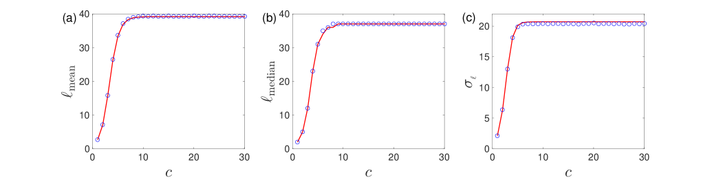
Figure 3: The mean, $\ell_{\rm mean}$ (a), median, $\ell_{\rm median}$ (b) and the standard deviation $\sigma_{\ell}$ (c), of the distribution of first hitting times of RWs on directed ER networks of size $N=1000$, as a function of the mean degree, $c$. The analytical results (solid lines), obtained from Eqs. (39), (40) and (44), respectively, are in excellent agreement with numerical simulations (circles).

To obtain a more complete characterization of the distribution of first hitting times, it is also useful to evaluate its median, $\ell_{\rm median}$. Here the median is defined as the value of $\ell$ for which $|P(d>\ell)-P(d<\ell)|\rightarrow{\rm min}$, where $\ell$ may take either an integer or a half-integer value. For integer values of $\ell$, $P(d<\ell)=1-P(d>\ell-1)$ while for half integar values of $\ell$, $P(d<\ell)=1-P(d>\ell)$. Expressing $P(d>\ell)$ by Eq. (31), we find that $\ell_{\rm median}$ can be approximated by

$$\ell_{median}\simeq\frac{1}{2}\left\lfloor 4\alpha\sqrt{\alpha^{2}\beta^{2}+\ln 2}-4\alpha^{2}\beta+1/2\right\rfloor,$$ (40)

where $\lfloor x\rfloor$ is the largest integer which is smaller than $x$. For small values of $c$, the median, $\ell_{\rm median}$ quickly increases as $c$ is increased, until it saturates. The saturation is obtained at $c\simeq(\ln N)/2$. The saturation value of $\ell_{\rm median}$ is $\ell_{\rm median}\simeq\lceil\sqrt{2N\ln 2}\rceil$, which is slightly lower than the saturation value of $\ell_{\rm mean}$. In Fig. 3(b) we present analytical results (solid lines) for the median, $\ell_{\rm median}$, as a function of the mean degree $c$. The analytical results are found to be in very good agreement with the results of numerical simulations (circles).

The moments of the distribution of RW path lengths, $\langle\ell^{n}\rangle$, are given by the tail-sum formula [31]

$$\langle\ell^{n}\rangle=\sum_{\ell=0}^{N-2}[(\ell+1)^{n}-\ell^{n}]P(d>\ell).$$ (41)

Using this formula to evaluate the second moment and replacing the sum by an integral we obtain

$$\langle\ell^{2}\rangle=1+\int_{\frac{1}{2}}^{N-\frac{3}{2}}\left(2\ell+1\right)\exp\left[-\left(\frac{\ell}{2\alpha}\right)^{2}-\beta\ell\right]d\ell.$$ (42)

Solving the integral and taking the limit $N\gg 1$, we obtain

$$\langle\ell^{2}\rangle=1+\alpha e^{\alpha^{2}\beta^{2}}\left\{\sqrt{\pi}\left(1-4\alpha^{2}\beta\right)\left[1-{\rm erf}\left(\frac{1+4\alpha^{2}\beta}{4\alpha}\right)\right]+4\alpha e^{-\left(\frac{1+4\alpha^{2}\beta}{4\alpha}\right)^{2}}\right\}.$$ (43)

The standard deviation $\sigma_{\ell}(c)$ is given by

$$\sigma_{\ell}^{2}(c)=\langle\ell^{2}\rangle-\ell_{mean}^{2}.$$ (44)

For small values of $c$, the standard deviation, $\sigma_{\ell}$, quickly increases as $c$ is increased, until it saturates. The saturation level of the standard deviation is $\sigma_{\ell}\simeq\sqrt{(4-\pi)N/2}$. In Fig. 3(c) we present analytical results (solid lines) for the standard deviation, $\sigma_{\ell}$, as a function of the mean degree $c$. The analytical results are found to be in very good agreement with the results of numerical simulations (circles).

8 Analysis of the two termination mechanisms

The path of an RW on a directed ER network may terminate either by the trapping scenario or by the retracing scenario. Since the initial node is chosen such that its out-degree satisfies $k_{out}\geq 1$, the trapping mechanism may occur starting from the second step of the RW. The probability of trapping is $\exp(-c)$ at any time step afterwards. The termination by retracing takes place when the RW steps into a node which it has already visited before. This may also occur starting from the second time step of the RW. The probability that an RW will terminate by retracing increases with time. This is due to the fact that each visited node becomes a potential termination site. In the limit of sparse networks, paths which terminate after a small number of steps are likely terminate by trapping, while paths which survive for a long time are more likely to terminate by retracing. In denser networks the probability of termination by trapping is much lower than the probability of termination by retracing even for short paths. Below we present a detailed analysis of the probabilities of an RW to terminate by trapping or by retracing. We denote by $p_{\rm trap}$ the probability that an RW starting from a random initial node will eventually terminate by the trapping scenario and by $p_{\rm ret}$ the probability that it will terminate by the retracing scenario. These two probabilities satisfy $p_{\rm trap}+p_{\rm ret}=1$.

It is of interest to study the conditional distributions, $P(d=\ell|{\rm trap})$, of paths terminated by trapping, and $P(d=\ell|{\rm ret})$, of paths terminated by retracing. These distributions satisfy the normalization conditions $\sum_{\ell=2}^{N-1}P(d=\ell|{\rm trap})=1$ and $\sum_{\ell=2}^{N-1}P(d=\ell|{\rm ret})=1$. The overall distribution of path lengths can be decomposed in terms of the conditional distributions according to

$$P(d=\ell)=p_{\rm trap}P(d=\ell|{\rm trap})+p_{\rm ret}P(d=\ell|{\rm ret}).$$ (45)

The first term on the right hand side of Eq. (45) can be written as

$$p_{\rm trap}P(d=\ell|{\rm trap})=P(d>\ell-1)\left[1-P_{\rm trap}(d>\ell|d>\ell-1)\right],$$ (46)

namely as the probability that the RW will pursue $\ell$ steps and will terminate at the $\ell+1$ step by the trapping scenario. The second term on the right hand side of Eq. (45) can be written as

$$p_{\rm ret}P(d=\ell|{\rm ret})=P(d>\ell-1)P_{\rm trap}(d>\ell|d>\ell-1)\left[1-P_{\rm ret}(d>\ell|d>\ell-1)\right],$$ (47)

namely as the probability that the RW will pursue $\ell$ steps, then in the $\ell+1$ step it will not get trapped but will retrace its path by stepping into a node which was already visited before. Summing up both sides of Eq. (46) over all integer values of $\ell$ we conclude that

$$p_{\rm trap}=e^{-c}\sum_{\ell=1}^{N-1}P(d>\ell-1).$$ (48)

Using the tail-sum formula, Eq. (35), we find that the probability that the RW will terminate by the trapping scenario is actually

$$p_{\rm trap}=e^{-c}\ell_{\rm mean}.$$ (49)

Therefore, the probability of the RW to terminate by retracing is

$$p_{\rm ret}=1-e^{-c}\ell_{\rm mean}.$$ (50)

In Fig. 4 we present the probability $p_{\rm trap}$ that an RW on a directed ER network of size $N=1000$ will terminate by trapping and the probability $p_{\rm ret}$ that it will terminate by retracing, as a function of the mean degree, $c$. As expected, the probability $p_{\rm trap}$ is a decreasing function of $c$ while $p_{\rm ret}$ is an increasing function of $c$.

Figure 4: The probabilities $p_{\rm trap}$ and $p_{\rm ret}$ that an RW on a directed ER network will terminate by trapping or by retracing, respectively, as a function of the mean degree, $c$. The theoretical results, obtained from Eqs. (49) and (50) are found to be in excellent agreement with the results of numerical simulations (symbols).

Using Eq. (46) the conditional probability $P(d=\ell|{\rm trap})$ can be written in the form

$$P(d=\ell|{\rm trap})=\frac{P(d>\ell-1)}{\ell_{\rm mean}},$$ (51)

where $P(d>\ell-1)$ is given by Eq. (31). Similarly, the conditional probability $P(d=\ell|{\rm ret})$ takes the form

$$P(d=\ell|{\rm ret})=\left(\frac{1-e^{-c}}{c}\right)\left[\frac{c-c(\ell)}{1-e^{-c}\ell_{\rm mean}}\right]P(d>\ell-1),$$ (52)

where $c(\ell)$ is given by Eq. (6). The corresponding tail distributions take the form

$$P(d>\ell|{\rm trap})=\frac{\sum_{t=\ell+1}^{N-1}P(d>t-1)}{\ell_{\rm mean}},$$ (53)

and

$$P(d>\ell|{\rm ret})=\left(\frac{1-e^{-c}}{c}\right)\sum_{t=\ell+1}^{N-1}\left[\frac{c-c(t)}{1-e^{-c}\ell_{\rm mean}}\right]P(d>t-1).$$ (54)

Replacing the sums in Eqs. (53) and (54) by integrals and carrying out the integrations, we obtain

$$P(d>\ell|{\rm trap})\simeq\frac{\sqrt{\pi}\alpha e^{\alpha^{2}\beta^{2}}\left[1-{\rm erf}\left(\frac{2\alpha^{2}\beta+\ell-1/2}{2\alpha}\right)\right]}{1+\sqrt{\pi}\alpha e^{\alpha^{2}\beta^{2}}\left[1-{\rm erf}\left(\frac{4\alpha^{2}\beta+1}{4\alpha}\right)\right]},$$ (55)

and

$$P(d>\ell|{\rm ret}) \simeq \left[\frac{1-e^{-c}}{\left(1-e^{-c}\ell_{\rm mean}\right)N}\right]\left\{2\alpha^{2}e^{-\frac{(\ell-1/2)^{2}}{4\alpha^{2}}-\beta(\ell-1/2)}\right.$$ (56)

$$- \left.\sqrt{\pi}\alpha(2\alpha^{2}\beta-1)e^{\alpha^{2}\beta^{2}}\left[1-{\rm erf}\left(\frac{2\alpha^{2}\beta+\ell-1/2}{2\alpha}\right)\right]\right\}.$$

In Fig. 5 we present the probabilities $P(d>\ell|{\rm trap})$ and $P(d>\ell|{\rm ret})$ that the path of an RW on a directed ER network will be of length larger than $\ell$, given that it terminated by trapping or by retracing, respectively. The results are presented for $N=1000$ and $c=3$, $5$ and $7$. The analytical results (solid lines) are found to be in excellent agreement with the numerical simulations (symbols). In both cases, the paths tend to become longer as $c$ is increased. However, for each value of $c$, the paths which terminate due to retracing are typically longer than the paths which terminate due to trapping.

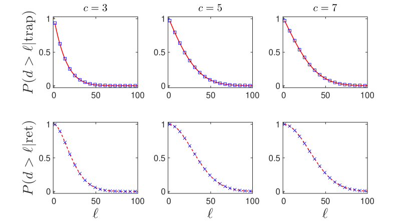
Figure 5: The conditional tail distributions $P(d>\ell|{\rm trap})$ and $P(d>\ell|{\rm ret})$ of first hitting times vs. $\ell$ for RWs on a directed ER network, for paths terminated by trapping (top row) or by retracing (bottom row), respectively. The results are shown for $N=1000$ and $c=3$, $5$ and $7$. The theoretical results for $P(d>\ell|{\rm trap})$ are obtained from Eq. (53), while the theoretical results for $P(d>\ell|{\rm ret})$ are obtained from Eq. (54). In both cases, the theoretical results (solid lines) are found to be in excellent agreement with the numerical simulations (symbols).

Given that the path of an RW has terminated after $\ell$ steps, it is interesting to evaluate the conditional probabilities $P({\rm trap}|d=\ell)$ and $P({\rm ret}|d=\ell)$, that the termination was caused by trapping or by retracing, respectively. Using Bayes’ theorem, these probabilities can be expressed by

$$P({\rm trap}|d=\ell)=\frac{p_{\rm trap}P(d=\ell|{\rm trap})}{P(d=\ell)},$$ (57)

and

$$P({\rm ret}|d=\ell)=\frac{p_{\rm ret}P(d=\ell|{\rm ret})}{P(d=\ell)}.$$ (58)

Clearly, these distributions satisfy $P({\rm trap}|d=\ell)+P({\rm ret}|d=\ell)=1$. Inserting the conditional probabilities $P(d=\ell|{\rm trap})$ and $P(d=\ell|{\rm ret})$ from Eqs. (51) and (52), respectively, we find that

$$P({\rm trap}|d=\ell)=\frac{P(d>\ell-1)}{e^{c}P(d=\ell)},$$ (59)

and

$$P({\rm ret}|d=\ell)=\left(1-e^{-c}\right)\frac{\left[c-c(\ell)\right]}{c}\frac{P(d>\ell-1)}{P(d=\ell)}.$$ (60)

The corresponding distributions can be expressed in the form

$$P({\rm trap}|d>\ell)=\frac{\sum\limits_{t=\ell+1}^{N-1}P(d>t-1)}{e^{c}P(d>\ell)},$$ (61)

and

$$P({\rm ret}|d>\ell)=\left(\frac{1-e^{-c}}{c}\right)\sum_{t=\ell+1}^{N-1}\left[c-c(t)\right]\frac{P(d>t-1)}{P(d>\ell)}.$$ (62)

These distributions also satisfy $P({\rm trap}|d>\ell)+P({\rm ret}|d>\ell)=1$. In Fig. 6 we present the probabilities $P({\rm trap}|d>\ell)$ and $P({\rm ret}|d>\ell)$ that an RW path on a directed ER network will terminate due to trapping or retracing, respectively, given that its length is larger than $\ell$. Results are shown for directed ER networks of size $N=1000$ and $c=3$, $5$ and $7$. The theoretical results for $P({\rm trap}|d>\ell)$ (solid lines) are obtained from Eq. (61) while the theoretical results for $P({\rm ret}|d>\ell)$ (dashed lines) are obtained from Eq. (62). As expected, it is found that $P({\rm trap}|d>\ell)$ is a monotonically decreasing function of $\ell$ while $P({\rm ret}|d>\ell)$ is monotonically increasing. In the top row these results are compared to the results of numerical simulations (symbols) finding excellent agreement. This comparison is done for the range of path lengths which actually appear in the numerical simulations. Longer RW paths which extend beyond this range become extremely rare, so it is difficult to obtain sufficient numerical data. However, in the bottom row we show the theoretical results for a larger range of path lengths. As can be seen, for small values of $c$, the curves of $P({\rm trap}|d>\ell)$ and $P({\rm ret}|d>\ell)$ cross each other, while for larger values of $c$ there is no such crossing. In fact, long paths can be sampled using the pruned enriched Rosenbluth method, which was successfully used in the context of SAWs in polymer physics [32]. In this method one samples long non-overlapping paths, keeping track of their weights, to obtain an unbiased sampling in the ensemble of all paths.

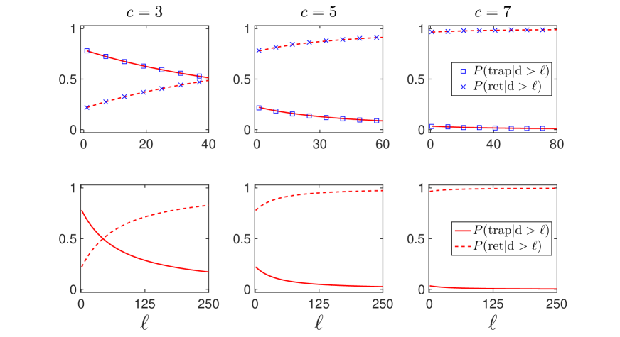
Figure 6: The conditional probabilities, $P({\rm trap}|d>\ell)$ and $P({\rm ret}|d>\ell)$, that an RW path on a directed ER network will terminate by trapping or by retracing, respectively, given that its length is larger than $\ell$, are presented as a function of $\ell$. Results are shown for an ER networks of size $N=1000$ and $c=3$, $5$ and $7$. The theoretical results for $P({\rm trap}|d>\ell)$ (solid lines) are obtained from Eq. (61) while the theoretical results for $P({\rm ret}|d>\ell)$ (dashed lines) are obtained from Eq. (62). In the top row these results are compared to the results of numerical simulations (symbols) finding excellent agreement. This comparison is done for the range of path lengths which actually appear in the numerical simulations and for which good statistics can be obtained. Longer RW paths which extend beyond this range become extremely rare, so it is difficult to obtain sufficient numerical data. However, in the bottom row we show the theoretical results for a larger range of path lengths. It is found that $P({\rm trap}|d>\ell)$ is a monotonically decreasing function of $\ell$ while $P({\rm ret}|d>\ell)$ is monotonically increasing.

9 The distribution of first hitting times on directed semi-ER networks

In most of the directed networks encountered in nature the distribution of in-degrees differs from the distribution of out-degrees. It is thus important to disentangle the effects of the in-degrees and out-degrees on the distribution of first hitting times. To this end, we extend out studies to a class of directed networks, referred to as directed semi-ER networks in which the in-degrees follow a Poisson distribution, whose mean is equal to $c$, as is the case in directed ER networks. However, the out-degrees may be distributed according to any desired distribution with the same mean, $c$. It is important to note that in the models studied here there are no correlations between the in-degree and the out-degree of any given node. Also, there are no degree-degree correlations between adjacent nodes. They thus belong to the class of directed configuration model networks [25, 33, 34, 35, 36, 37].

To construct an instance of a network from a given ensemble of directed configuration model networks of $N$ nodes, one draws the in-degrees and out-degrees from the desired distributions $p^{\rm in}(k)$ and $p^{\rm out}(k)$, $k=0,1,\dots,N-1$, producing the degree sequences $k_{i}^{\rm in}$, and $k_{i}^{\rm out}$, $i=1,\dots,N$. While the distributions must satisfy the condition $\sum_{k}kp^{\rm in}(k)=\sum_{k}kp^{\rm out}(k)$, for each instance one needs to make sure that $\sum_{i}k_{i}^{\rm in}=\sum_{i}k_{i}^{\rm out}$. One then prepares the $N$ nodes such that each node, $i$, is connected to $k_{i}^{\rm in}$ incoming half links and $k_{i}^{\rm out}$ outgoing half links [34]. Pairs of an incoming half link from one node and an outgoing half link from another node are then chosen randomly and are connected to each other in order to form the network. The result is a network with the desired degree sequence and no correlations. Note that towards the end of the construction the process may get stuck. This may happen in case that the only remaining pairs of half links are in the same node or in nodes which are already connected to each other. In such cases one may perform some random reconnections in order to enable completion of the construction.

The directed semi-ER networks can be constructed using a simpler procedure than the general configuration model networks. Consider the adjacency matrix, $A$, of a directed semi-ER network of size $N$. The matrix element $a_{ij}=1$ if there is a directed link from node $i$ to node $j$, and zero otherwise. The diagonal elements, $a_{ii}=0$, for all $i=1,2,\dots,N$. The first step in the construction is to draw the sequence of out-degrees, $k_{i}^{\rm out}$, $i=1,2,\dots,N$ from the distribution $p^{\rm out}(k)$. The $i$th row of $A$ thus includes $k_{i}^{\rm out}$ 1’s and $N-k_{i}^{\rm out}$ 0’s. In the second step, one places randomly the $k_{i}^{\rm out}$ $1$’s among the $N-1$ non-diagonal matrix elements of the $i$th row. Since there are no correlations between the placements of 1’s in different rows, the in-degrees follow a Poisson distribution whose mean is equal to $c$. In this procedure there is no need for any adjustments since the total number of incoming links is directly determined by the number of outgoing links.

Below we consider several examples of directed semi-ER networks. In case that the out-degrees also follow the Poisson distribution, the directed ER network is recovered. For integer values of $c$, the out-degrees may follow a degenerate distribution, in which the out-degrees $k_{i}^{\rm out}=c$ for all the nodes in the network. Such networks may be considered as a hybridization of an ER network and a regular graph [20]. Clearly, in these networks there are no dead-end nodes of degree $k_{i}^{\rm out}=0$.

Another interesting example is the case in which the out-degrees follow a power-law distribution of the form

$$p^{\rm out}(k)=Ak^{-\gamma},$$ (63)

for $k_{\rm min}\leq k\leq k_{\rm max}$, where the lower cutoff $k_{min}\geq 1$ and an upper cutoff $k_{max}\leq N-1$. Such distributions are also known as scale-free distributions. The normalization coefficient, $A$ is given by

$$A=\frac{1}{\zeta(\gamma,k_{min})-\zeta(\gamma,k_{max}+1)},$$ (64)

where $\zeta(s,a)$ is the Hurwitz zeta function [26]. The mean of the out-degree distribution, $\langle k\rangle^{\rm out}=\sum_{k}kp^{\rm out}(k)$, is given by

$$\langle k\rangle^{\rm out}=\frac{\zeta(\gamma-1,k_{min})-\zeta(\gamma-1,k_{max}+1)}{\zeta(\gamma,k_{min})-\zeta(\gamma,k_{max}+1)}.$$ (65)

In case that $k_{\rm min}=1$ the Hurwitz zeta function $\zeta(s,1)$, coincides with the Riemann zeta function, $\zeta(s)$ [26]. Therefore, in this case the mean of the out-degree distribution is given by

$$\langle k\rangle^{\rm out}=\frac{\zeta(\gamma-1)-\zeta(\gamma-1,k_{max}+1)}{\zeta(\gamma)-\zeta(\gamma,k_{max}+1)}.$$ (66)

Since $\langle k\rangle^{\rm out}=c$, one can use Eq. (66) in order to obtain the value of the exponent $\gamma$ which would yield the desired mean out-degree, $c$. Such a directed semi-ER network with a Poisson in-degree distribution and a power-law out-degree distribution can be considered as a hybridization of an ER network and a scale-free network [38]. Since $k_{\rm min}=1$, these networks do not include any dead end nodes of degree $k_{i}^{\rm out}=0$.

We also consider the case in which the out-degrees follow an exponential distribution of the form

$$p^{\rm out}(k)=Be^{-\alpha k},$$ (67)

in the range $k_{\rm min}\leq k\leq k_{\rm max}$, where the lower cutoff is $k_{\rm min}=0$ and the upper cutoff is $k_{\rm max}\leq N-1$. The normalization factor, $B$, is given by

$$B=\frac{1-e^{-\alpha}}{1-e^{-\alpha(k_{\rm max}+1)}}.$$ (68)

Due to the fast decay of the exponential distribution, we can take the approximation in which $k_{\rm max}\rightarrow\infty$. In this case the normalization factor is simplified to $B=1-e^{-\alpha}$. Within this approximation, the mean of the exponential out-degree distribution is given by

$$\langle k\rangle^{\rm out}=\frac{1}{e^{\alpha}-1}.$$ (69)

Since $\langle k\rangle^{\rm out}=c$, we find that in order to obtain a desired value of the mean out-degree, $c$, the exponent $\alpha$ of the exponential out-degree distribution should be given by

$$\alpha=\ln\left(\frac{c+1}{c}\right).$$ (70)

The fraction of nodes in these networks which are dead-end nodes of zero out-degree is given by $p^{\rm out}(k=0)=B$, which in the limit of large $k_{\rm max}$ is well approximated by

$$p^{\rm out}(k=0)=1-e^{-\alpha}.$$ (71)

In order to calculate the distribution of first hitting times of RWs on directed semi-ER networks we recall that the probability that an RW will visit node $i$, which resides on the subnetwork of the yet-unvisited nodes, is proportional to its in-degree, $k_{i}^{\rm in}(t)$. The expectation value of the number of incoming links of the node visited by the RW at time $t$, which originate from the subnetwork of the yet-unvisited nodes, are removed at that time is $c(t)$. Since the distribution of out-degrees is uncorrelated with the distribution of in-degrees, the expectation value of the number of outgoing links from the node visited at time $t$ to the subnetwork the yet-unvisited nodes, which are then removed, is also given by $c(t)$. Therefore, the analysis presented in Sec. 4, which is based on special properties of the Poisson distribution, still holds for the in-degree distribution, which remains Poisson, and its mean, $c(t)$ is given by Eq. (6).

The probability of not terminating by retracing at time $t$, $P_{\rm ret}(d>t|d>t-1)$, given by Eq. (19), is equal to the ratio between the mean degree $c(t)$ of the subnetwork of the yet-unvisited nodes and the mean degree of the entire network, $c$. Since the time evolution of $c(t)$ is not affected by the out-degree distribution, the probability of termination by retracing remains identical to the case of an ER network with the same value of $c$.

For RWs on a directed ER network, the probability of not terminating by trapping, $P_{\rm trap}(d>t|d>t-1)$, given by Eq. (17), is independent of the time, $t$. For RWs on directed semi-ER networks, it is replaced by

$$P_{\rm trap}(d>t|d>t-1)=1-p^{\rm out}(k=0),$$ (72)

where $p^{\rm out}(k=0)$ is the probability that a randomly chosen node in the network is a dead-end node which does not have any outgoing links. Since this probability does not evolve in time, it can be determined from the initial distribution $p^{\rm out}(k)$. As shown above, for the degenerate distribution and for the power-law distribution the probability $p^{\rm out}(k=0)=0$. Therefore, the trapping scenario does not apply to RWs on these networks and their paths terminate only by retracing. On the other hand, for the exponential distribution the probability $p^{\rm out}(k=0)$ is non-zero and is given by Eq. (71). Thus, for the network with an exponential degree distribution, $P_{\rm trap}(d>\ell)=\exp(-b\ell)$, where $b=-\ln[1-p^{\rm out}(k=0)]$.

In Fig. 7 we present the tail distributions of first hitting times, $P(d>\ell)$, of RWs on three directed semi-ER networks, all of them of size $N=1000$ and $c=5$. In these networks the in-degrees follow a Poisson distribution, while the out-degrees are distributed according to a degenerate (regular) distribution (a), a power-law (scale-free) distribution, which is obtained using the parameters $\gamma=2.14$ and $k_{\rm min}=1$ (b), and an exponential distribution, obtained using the parameters $\alpha=0.18$ and $k_{\rm min}=0$ (c). The analytical results (solid lines) are in excellent agreement with the results obtained from numerical simulations (circles).

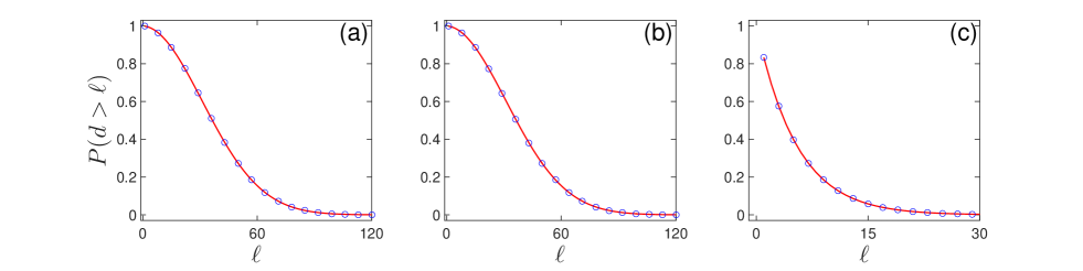
Figure 7: The tail distributions of first hitting times, $P(d>\ell)$, of RWs on directed semi-ER networks of size $N=1000$ and $c=5$, in which the in-degrees follow the Poisson distribution and the out-degrees are distributed according to a degenerate (regular) distribution (a), a power-law (scale-free) distribution with $\gamma=2.14$ and $k_{\rm min}=1$ (b), and an exponential distribution with $\alpha=0.18$ and $k_{\rm min}=0$ (c). The analytical results (solid lines) are in excellent agreement with the results obtained from numerical simulations (circles).

-

In Fig. 8 we present analytical results for the tail distributions of first hitting times, $P(d>\ell)$, of RWs on directed semi-ER networks of size $N=1000$ and $c=5$, in which the out-degrees are distributed according to a Poisson distribution (solid line), an exponential distribution (dotted line) as well as a degenerate distribution (regular graph) and a power-law distribution (which coincide with each other and shown by a dashed line). The results for the degenerate distribution and the power-law distribution are identical. This is due to the fact that in both networks the termination scenario by trapping does not exist, while the termination probabilities by retracing are identical in the two networks. This result is surprising in light of the fact that the degenerate distribution and the power-law distribution are entirely different from each other. In particular, the degenerate distribution is infinitely narrow, while the power-law distribution exhibits a broad tail and for $\gamma\leq 3$ its variance diverges.

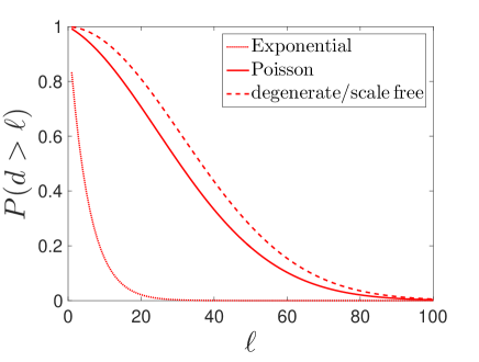
Figure 8: Analytical results for the tail distributions of first hitting times, $P(d>\ell)$, of RWs on four directed networks of size $N=1000$ and $c=5$: a directed ER network (solid line), in which both the in-degrees and the out-degrees follow a Poisson distribution, and three directed semi-ER networks, in which the in-degrees follow a Poisson distribution and the out-degrees are distributed according to an exponential distribution (dotted line), with $\alpha=0.18$ and $k_{\rm min}=0$, a degenerate (regular) distribution (dashed line), and a power-law (scale-free) distribution (dashed line), with $\gamma=2.14$ and $k_{\rm min}=1$. The results obtained for the two latter distributions are identical, and thus shown by the same dashed line.

The RW paths on networks with Poisson and exponential out-degree distributions may terminate either by retracing or by trapping. The network with an exponential out-degree distribution exhibits a much larger fraction of dead-end nodes. Therefore the first hitting times of RWs on this network are much shorter than on the network with a Poisson out-degree distribution (which is, in fact, an undirected ER network).

10 Summary and discussion

We presented analytical results for the distribution of first hitting times of RWs on directed ER networks. Starting from a random initial node, these RWs hop randomly along directed edges between adjacent nodes until their paths terminate. Termination may occur either by retracing or by trapping. In the retracing scenario the RW steps into a node which it has already visited before. In the trapping scenario the RW becomes trapped in a ’dead-end’ node which has no outgoing edges. The number of steps pursued from the initial node up to the termination of the RW path is called the first hitting time. Using recursion equations we obtained analytical results for the tail distribution of first hitting times, $P(d>\ell)$ as well as for the mean, median and standard deviation of this distribution. The results are found to be in excellent agreement with numerical simulations. It was found that the tail distribution $P(d>\ell)$ can be expressed as a product of an exponential distribution and a Rayleigh distribution.

In Fig. 9 we present analytical results (solid line) for the tail distribution of first hitting times, $P(d>\ell)$, of RWs on a directed ER network of size $N=1000$ and $c=4$. For comparison we also present the corresponding distribution of RWs on an undirected ER network (dashed line) with the same value of $c$ (based on Ref. [13]). It is found that the first hitting times of RWs on directed ER networks are much longer than those of RWs on undirected ER networks. This is due to the fact that in undirected networks the backtracking scenario is a dominant termination mechanism which contributes to a significant reduction in the first hitting times.

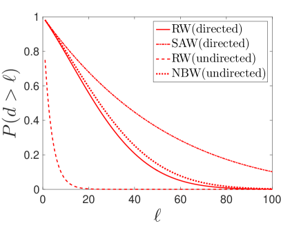
Figure 9: Analytical results for the tail distribution of first hitting times, $P(d>\ell)$, of RWs on a directed ER network (solid line), obtained from Eq. (28). For comparison we also present the tail distribution of first hitting times of RWs on an undirected ER network (dashed line), obtained using the analytical expression derived in Ref. [13], as well as of NBWs on undirected ER networks (dotted line), obtained using the analytical expression derived in Ref. [39]. In all three cases the network size is $N=1000$ and $c=4$. It is found that the first hitting times of RWs on directed ER networks are much longer than those of RWs on undirected networks. This is due to the fact that in undirected ER the backtracking scenario is a dominant termination mechanism, while in directed ER network this scenario does not exist and is replaced by the trapping scenario which is much weaker. The first hitting times of NBWs on undirected ER networks are found to be slightly longer than those of RWs on directed ER networks. The distribution of last hitting times of SAWs on a directed ER network, obtained from Eq. (13), is also shown (dashed-dotted line). As expected, the last hitting times are significantly longer than the first hitting times on the same network.

For the sake of completeness, we briefly summarize the properties of first hitting times of RWs on undirected ER networks. The conditional probability associated with the retracing scenario of RWs on undirected ER networks is given by

$$P_{\rm ret}(d>t|d>t-1)=\frac{c(t)+1}{c+1}.$$ (73)

This probability is somewhat larger than the result for directed ER networks, given by Eq. (19). However, the main difference between the distributions of first hitting times in the directed and undirected ER networks is the fact that on directed networks the backtracking scenario does not exist. The conditional probability associated with the backtracking scenario for RWs on undirected ER networks is given by [13]

$$P_{\rm backtrack}(d>t|d>t-1)=\frac{c-1+e^{-c}}{c}.$$ (74)

Thus, backtracking is an important termination scenario, particularly for sparse networks. Unlike the case of undirected networks, in directed ER networks the backtracking scenario does not exist because the backwards link to the previous node exists only with probability $p$, namely it is as likely as a link to any other node. However, another termination scenario emerges. This is the trapping scenario, which occurs when the RW enters a dead-end node which does not have any outgoing link and becomes trapped in that node. It turns out that the trapping scenario in directed ER networks is much less likely to happen than the backtracking scenario in the corresponding undirected ER network. The conditional probability associated with the trapping scenario for RWs on directed ER networks is given by

$$P_{\rm trap}(d>t|d>t-1)=1-e^{-c}.$$ (75)

Note that both the backtracking and trapping probabilities do not depend on time. However, their dependencies on the mean degree, $c$ is very different from each other. While the backtracking probability essentially decreases as $1/c$, the trapping probability decreases exponentially with $c$. Therefore, the trapping mechanism is much less likely to occur and so the paths of RWs on directed ER networks are much longer than on a corresponding undirected networks with the same value of $c$.

The properties of RWs on directed ER networks resemble those of non-backtracking RWs (NBWs) on undirected ER networks [39]. This is due to the fact that in both cases the termination of the RW path by the backtracking scenario is suppressed. In Fig. 9 we also show the tail distribution of NBWs on undirected ER networks (dotted line). Indeed, it is found to be very similar to the tail distribution of RWs on directed ER networks. However, the tail distribution of the NBWs is shifted slightly to the right compared to the tail distribution of the corresponding RW on a directed ER network. This is due to the fact that the probability of retracing is slightly lower for the NBW compared to the RW on a directed ER network. More precisely, for an NBW on an undirected ER network the probability of retracing at the $t+1$ time step is given by $[c-c(t)]/(c+1)$, compared to $[c-c(t)]/c$ for an RW on a directed ER networks. For completeness, we also show in Fig. 9 the distribution of last hitting times of SAWs on directed ER networks (dashed-dotted lines), obtained from Eq. (14). As expected, the last hitting times are much longer than the first hitting times.

We performed a detailed analysis of the probabilities, $p_{\rm trap}$ and $p_{\rm ret}$, that the termination will take place via the trapping or via the retracing mechanism, respectively. We obtained analytical expressions for these probabilities in terms of the network size, $N$, and the mean degree, $c$. We also obtained analytical expressions for the conditional distributions of the path lengths, $P(d=\ell|{\rm trap})$ and $P(d=\ell|{\rm ret})$ for the paths which terminate by trapping or by retracing, respectively. Finally, we obtained analytical expressions for the conditional probabilities $P({\rm trap}|d=\ell)$ and $P({\rm ret}|d=\ell)$ that a path which terminates after $\ell$ steps is terminated by trapping or by retracing, respectively. It was found that the two termination mechanisms exhibit very different behavior. Since the initial node is chosen to be a node with at least one outgoing link, the trapping probability sets in starting from the second step. The trapping probability is constant throughout the path. As a result, the trapping mechanism alone would produce a geometric distribution of path lengths. The retracing mechanism also sets in starting from the second step and its rate increases linearly in time. The balance between the two termination mechanisms depends on the mean degree of the network. In the limit of sparse networks, the trapping mechanism is dominant and most paths are terminated long before the retracing mechanism becomes relevant. In the case of dense networks, the trapping probability is low and most paths terminate by the retracing mechanism. These results provide useful insight into the general problem of survival analysis and the statistics of mortality or failure rates, under conditions in which two or more failure mechanisms coexist [40, 41].

We have shown that the approach developed in this paper applies not only to ER networks but also to directed semi-ER networks in which the in-degree distribution is a Poisson distribution while the out-degrees may follow any desired distribution which has the same mean, $c$, as the in-degree distribution. To demonstrate this result we presented the tail distribution, $P(d>\ell)$, for directed semi-ER networks with degenerate (regular), power-law (scale free) and exponential out-degree distributions. It was shown that the rate of termination by retracing is determined by the Poisson in-degree distribution, which controls the temporal evolution of $c(t)$. The rate of termination by trapping is determined by the out-degree distribution, or more specifically by the probability $p^{\rm out}(k=0)$ that a randomly chosen node will have no outgoing link.

In a broader context, the distributions of first hitting times and last hitting times of RWs are examples of a broad class of distributions of path lengths and first passage times in random networks [4]. A related distribution, which provides useful information on the underlying structure of the network, is the distribution of shortest path lengths between random pairs of nodes [25, 42, 43, 44, 45, 46, 47, 48, 49]. Examples of such distributions involving RWs are the distribution of first passage times between random pairs of nodes [7] and the distribution of cover times [8]. We expect the methodologies developed in this paper to be useful for the study of other structural and dynamical distributions in random networks.

11 Appendix A: Detailed calculation of $P_{\rm ret}(d>\ell)$

In this Appendix we present the detailed evaluation of $P_{\rm ret}(d>\ell)$. Taking the logarithm of $P_{\rm ret}(d>\ell)$, as expressed in Eq. (24), we obtain

$$\ln\left[P_{\rm ret}(d>\ell)\right]=\sum_{t=1}^{\ell}\ln\left[\frac{c(t)}{c}\right].$$ (76)

Replacing the sum by an integral we obtain

$$\ln\left[P_{\rm ret}(d>\ell)\right]=\int_{1/2}^{\ell+1/2}\ln\left[\frac{c\left(t\right)}{c}\right]dt.$$ (77)

Plugging in the expression for $c(t)$ from Eq. (6) and rearranging terms in the integrand we obtain

$$\ln\left[P_{\rm ret}\left(d>\ell\right)\right]=\int_{1/2}^{\ell+1/2}\ln\left[1-\frac{t}{\left(N-1\right)}\right]dt.$$ (78)

After integration, replacement of $N-1$ by $N$ and rearrangement of terms we obtain

$$P_{\rm ret}\left(d>\ell\right)\simeq\exp\left[\left(\ell+\frac{3}{2}-N\right)\ln\left(1-\frac{\ell+1/2}{N-1}\right)-\ell-\frac{1}{2}\right].$$ (79)

In approximating the sum of Eq. (76) by the integral of Eq. (77) we have used the formulation of the middle Riemann sum. Since the function $\ln[P_{\rm ret}(d>\ell)]$ is a monotonically decreasing function, the value of the integral is over-estimated by the left Riemann sum, $L(\ell)$, and under-estimated by the right Riemann sum, $R(\ell)$. The error involved in this approximation is thus bounded by the difference $\Delta(\ell)=L(\ell)-R(\ell)$, which satisfies $\Delta(\ell)=-\ln(1-\ell/N)$. Thus, the relative error in $P_{\rm ret}(d>\ell)$ due to the approximation of the sum by an integral is bounded by $\eta_{\rm SI}\sim\ell/N$. Comparing the values obtained from the sum and the integral over a broad range of parameters, we find that the pre-factor of the error is very small, so in practice the error introduced by approximation of the sum by an integral is negligible.

References

- [1] Lawler G F and Limic V 2010 Random Walk: A Modern Introduction (Cambridge: Cambridge University Press)
- [2] Rudnick J and Gaspari G 2010 Elements of the Random Walk: An introduction for Advanced Students and Researchers (Cambridge: Cambridge University Press)
- [3] van Kampen N G 2007 Stochastic Processes in Physics and Chemistry (Amsterdam: North Holland)
- [4] Redner S 2001 A Guide to First Passage Processes (Cambridge: Cambridge University Press)
- [5] Montroll E E and Weiss G H 1965 J. Math. Phys. 6 167
- [6] De Bacco C, Majumdar S N and Sollich P 2015 J. Phys. A 48 205004
- [7] Sood V, Redner S and ben-Avraham D 2005 J. Phys. A 38 109
- [8] Kahn J D, Linial N, Nisan N and Saks M E 1989 J. Theor. Probab. 2 121
- [9] Herrero C P and Saboyá M 2003 Phys. Rev. E 68 026106
- [10] Herrero C P 2005 Phys. Rev. E 71 016103
- [11] Herrero C P 2005 J. Phys. A 38 4349
- [12] Herrero C P 2007 Eur. Phys. J. B. 56 71
- [13] Tishby I, Biham O and Katzav E 2016 J. Phys. A 50 115001
- [14] Erdős P and Rényi 1959 Publ. Math. 6 290
- [15] Erdős P and Rényi 1960 Publ. Math. Inst. Hung. Acad. Sci. 5 17
- [16] Erdős P and Rényi 1961 Bull. Inst. Int. Stat. 38 343
- [17] Madras N and Slade G 1996 The Self Avoiding Walk (Boston: Birkhäuser)
- [18] Slade G 2011 Surveys in Stochastic Processes, Proceedings of the 33rd SPA Conference in Berlin, 2009, EMS Series of Congress Reports, eds. Blath J, Imkeller P, and Roelly S
- [19] Tishby I, Biham O and Katzav E 2016 J. Phys. A 49 285002
- [20] Bollobas B 2001 Random Graphs, Second Edition (London: Academic Press)
- [21] Bang-Jensen J and Gutin G 2007 Digraphs Theory, Algorithms and Applications (Berlin: Springer-Verlag)
- [22] Graham A J and Pike D A 2008 Atlantic Electronic Journal of Mathematics 3, 1
- [23] Havlin S and Cohen R 2010 Complex Networks: Structure, Robustness and Function (Cambridge University Press, New York).
- [24] Dorogovtsev S N, Mendes J F F and Samukhin A N 2001 Phys. Rev. E 64 025101
- [25] Newman M E J, Strogatz S H and Watts D J 2001 Phys. Rev. E 64 026118
- [26] Olver F W J, Lozier D W, Boisvert R F and Clark C W 2010 NIST Handbook of Mathematical Functions (Cambridge: Cambridge University Press)
- [27] Gompertz B 1825 Philosophical Trans. R. Soc. London A 115 513
- [28] Johnson N L, Kotz S and Balakrishnan N 1995 Continuous Univariate Distributions (New York: John Wiley & Sons)
- [29] Shklovskii B I 2005 Theory in Biosciences 123 431
- [30] Ohishi K, Okamura H and Dohi T 2009 Journal of Systems and Software 82 535
- [31] Pitman J 1993 Probability (New York: Springer-Verlag)
- [32] Grassberger P 1997 Phys. Rev. E 56 3682
- [33] Molloy M and Reed B 1995 Random Struct. Algorithms 6 161
- [34] Newman M E J 2010 Networks: an Introduction (Oxford: Oxford University Press).
- [35] Fronczak A, Fronczak P and Holyst J A 2004 Phys. Rev. E 70 056110
- [36] Annibale A, Coolen A C C, Fernandes L P, Fraternali F and Kleinjung J 2009 J. Phys. A 42 485001
- [37] Roberts E S, Schlitt T and Coolen A C C 2011 J. Phys. A 44 275002
- [38] Albert R and Barabási A L 2002 Rev. Mod. Phys. 74 47
- [39] Tishby I, Biham O and Katzav E 2016 arXiv:1609.08375, accepted to J. Phys. A
- [40] Finkelstein M 2008 Failure Rate Modelling for Reliability and Risk (Springer-Verlag, London)
- [41] Gavrilov L A and Gavrilova N S 2001 J. theor. Biol 213 527
- [42] Blondel V D, Guillaume J -L, Hendrickx J M and Jungers R M 2007 Phys. Rev. E 76 066101
- [43] Dorogotsev S N, Mendes J F F and Samukhin A N 2003 Nuclear Physics B 653 307
- [44] van der Hofstad R, Hooghiemstra G and Znamenski D 2007 Electronic Journal of Probability 12 703
- [45] van der Hofstad R and Hooghiemstra G 2008 J. Math. Phys. 49 125209
- [46] van der Esker H, van der Hofstad R and Hooghiemstra G 2008 J. Stat. Phys. 133 169
- [47] Katzav E, Nitzan M, ben-Avraham D, Krapivsky P L, Kühn R, Ross N and Biham O 2015 EPL 111 26006
- [48] Nitzan M, Katzav E, Kühn R and Biham O 2016, Phys. Rev. E 93 062309
- [49] Melnik S and Gleeson J P 2016 arXiv:1604.05521