Stability Analysis of Multi-Period Electricity Market with Heterogeneous Dynamic Assets

Abstract

Market-based coordination of demand side assets has gained great interests in recent years. In spite of its efficiency, there is a risk that the interaction between the dynamic assets through the price signal could result in an unstable closed-loop system. This may cause oscillating power consumption profiles and high volatile energy price. This paper proposes an electricity market model which explicitly considers the heterogeneous dynamic asset models. We show that the market dynamics can be modeled by a discrete nonlinear system, and then derive analytical conditions to guarantee the stability of the market via contraction analysis. These conditions imply that the market stability can be guaranteed by choosing bidding functions with relatively shallower slopes in the linear region. Finally, numerical examples are provided to demonstrate the application of the derived stability conditions.

I Introduction

To adapt to the distributed generation and increasing penetration of volatile renewable energies and to improve the overall efficiency of the power industry, the power systems have undergone a substantial change from centrally controlled, vertically integrated organizations to decentrally controlled, deregulated systems. Market mechanism has been introduced at various levels of power systems to create competition. In particular, a local electricity market can be created to motivate self-interested distributed energy resources (DERs) to realize efficient energy allocation and achieve system-level objectives. Several demonstration projects have been implemented to validate the idea which showed promising practice. For example, the GridWise®  demonstration project by the Pacific Northwest National Laboratory showed that the market-based coordination of residential loads could reduce the utility demand and congestion at key times [8]. The AEP Ohio demonstration project [1] further showed the capability of enforcing both system-wide constraints and local constraints, while optimizing both system and individual objectives [28].

Motivated by these projects, recent studies have been focused on the market mechanism design for engaging different types of DERs [19, 11, 5, 18]. For example, the authors in [19] proposed a market mechanism to coordinate a population of thermostatically controlled loads (TCLs) for demand response. The proposed bidding strategies incorporated the TCL dynamics in order to improve the accuracy and efficiency of the load coordination. For commercial HVACs (heating, ventilation and air conditioning), a double-auction market structure was designed which takes into account the detailed nonlinear building models [11]. The proposed market was demonstrated to be very efficient at peak shaving and load shifting services. Other market models for demand response using batteries or PEVs (plug-in electric vehicles) were also proposed in [7, 18].

Despite the popularity of market-based coordination, there has been a growing concern about the risk of the instability of the power market. Under some extreme conditions, the aggregate demand and the energy price can be unstable or demonstrate high volatility over time. Various factors that contribute to the instability of market-coordinated TCLs have been examined in [24]. Some earlier works abstracted a simple linear differential equation model to quantify the power market stability [3, 2, 25]. A discrete time nonlinear model based on the marginal cost pricing mechanism was proposed in [27]. It assumed that the demand side did not bid into the market and its utility function was unknown to the system operator. The focus was therefore on the market instability caused by the uncertain demand prediction of the coordinator. Under the same framework of [27], the authors in [31] considered a more realistic dynamic consumption model. It was obtained from solving an optimal inventory control problem, and the market stability was found to be related to the ratio between the marginal backlog disutility and the marginal cost of supply.

The aforementioned works only considered aggregate demand models in autoregression form depending on the previous consumption history or price history [27, 31]. However, in order to quantify the aggregate demand variation more accurately, the internal dynamics and operational limits of individual DERs must be considered. More importantly, the impact of the population dynamics of the DERs on the overall market dynamics must be investigated systematically. These features are nevertheless abstracted away in the existing literature.

In this paper, we propose a market model which explicitly considers the individual dynamics of the DERs. Specifically, we model each DER by a general constrained linear system. Such models have been widely employed to describe the dynamics of its internal energy state [12, 29, 30]. Moreover, we consider the bidding process of the DERs and model the bidding functions to be dependent on the energy state. Consequently, the market is cleared at the competitive equilibrium, which results in an efficient energy allocation for each individual DERs. These features distinguish our work from those by [31, 27]: the latter of which assumed no bidding process and the price was ex-ante which may not clear the market.

Under the proposed market structure with heterogeneous dynamic DER models, we translate the analysis of the market stability into the stability analysis of a closed-loop system of the DER dynamics. In general, this system can be viewed as a model predictive control (MPC) system [22, 10] or systems with optimization based controller [13, 14, 26, 17]. By assuming quadratic utility and cost functions, it can be further shown to be a piecewise linear system [6]. Alternatively, it can be viewed as an input saturation system with state-dependent saturation limits. Most of the existing stability results considered only special cases of such systems [22, 13, 14, 26, 20, 15, 16], which are generally not applicable to the system considered in this paper. In fact, even the analysis of these much simpler systems are very challenging. While general numerical stability tests via Lyapunov methods may be employed, they lend little insights into the market practice. In addition, they are very conservative and can become intractable as the number of DERs increases.

To address the above challenges, we propose a contraction analysis based approach to analyzing the stability of such systems. This approach enables us to derive analytical conditions that guarantee the market stability. These conditions provide important insights into the design of the bidding functions. The key observation is that the market stability can be always guaranteed by selecting shallower bidding functions, that is, the linear region of the bidding function should have a relatively small slope. Moreover, these conditions are very mild, and thus leave the full freedom to the individual users to design their desired bidding functions while ensuring a stable electricity market.

The rest of this paper is organized as follows. The market structure and its equilibrium are described in Section II. The characterization of the equilibrium and the stability results are presented in Section III. Numerical examples illustrating the application of the stability results is provided in Section IV. Finally, the paper is concluded in Section IV.

Notation: We use ${\bf 1}_{m}$ to represent the $m$ dimensional column vector of all ones, and $I_{m}$ the $m$ dimensional identity matrix. The index set $\{1,2,...,m\}$ will be denoted by the $\mathcal{M}$. Let $\mathcal{X}$ be a subset of $\mathbb{R}^{m}$, then for $x\in\mathbb{R}^{m}$, the set $\mathcal{X}-x$ is defined as $\{x^{\prime}-x,\,\forall x^{\prime}\in\mathcal{X}\}$. For a symmetric matrix $S$, the inequality $S\succ 0$ ($S\succeq 0$ ) means that the matrix is positive definite (positive semi-definite). We denote by $\mathcal{H}_{Q}$ with $Q\succ 0$ the Hilbert space $\mathbb{R}^{m}$ with inner product $\left\langle\cdot,\cdot\right\rangle_{Q}:\,\mathbb{R}^{m}\times\mathbb{R}^{m}\mapsto\mathbb{R}$ defined as $\left\langle x,y\right\rangle_{Q}:=x^{T}Qy$, and induced norm $\left\|\cdot\right\|_{Q}:\,\mathbb{R}^{m}\mapsto\mathbb{R}_{\geq 0}$ defined as $\left\|x\right\|_{Q}:=\sqrt{x^{T}Qx}$. The Euclidean 2-norm will be denoted by $\left\|\cdot\right\|_{2}$, The projection operator in $\mathcal{H}_{Q}$, denoted by $\text{Proj}_{C}^{Q}(x):\,\mathbb{R}^{m}\mapsto C$, is defined as $\text{Proj}_{C}^{Q}(x):=\arg\min_{y\in C}\left\|x-y\right\|_{Q}=\arg\min_{y\in C}\left\|x-y\right\|_{Q}^{2}$. When $Q=I_{m}$, we simply write $\text{Proj}_{C}(x)$ which is the standard projection in $\mathbb{R}^{m}$.

II Problem Formulation

In this section, we will first describe an electricity market model which involves the bidding and clearing processes at each market period. The problem of market stability analysis is then defined formally.

II-A Market Structure

Usually a system coordinator is running an electricity market to schedule and guide the power usage of $m$ DERs. We assume that the $i$th DER is modeled by the following discrete time scalar linear system subject to both state and input constraints,

$$x_{i}^{+}=a_{i}x_{i}+d_{i},$$ (1)

where $x_{i}$, $x_{i}^{+}\in\mathcal{X}_{i}$ represent the current and the successive energy states of the DER, respectively, and $d_{i}\in\mathcal{D}_{i}$ is its power consumption. The state and input constraint sets will be denoted by $\mathcal{X}_{i}=[\underline{x}_{i},\bar{x}_{i}]$ and $\mathcal{D}_{i}=[\underline{d}_{i},\bar{d}_{i}]$, respectively. The constant $a_{i}\in(0,1]$ represents the energy dissipation rate. This model has been widely used to describe the power flexibility of the HVAC systems (when $a\in(0,1)$) or energy storage (when $a=1$), see for example, [12, 30, 29].

To ensure the controllability of the system (1), we impose the following conditions

$$a_{i}\underline{x}_{i}+\bar{d}_{i}>\underline{x}_{i},\,a_{i}\bar{x}_{i}+\underline{d}_{i}<\bar{x}_{i}.$$ (2)

Condition (2) guarantees that the DER can be controlled into $\mathcal{X}_{i}$ with $d_{i}\in\mathcal{D}_{i}$.

Note that the demand of the DER is changing dynamically with the current states. For example, the DER is less willing to procure power if its energy state is close to the upper bound. We assume that each DER submits a bid on the desired power and price to the coordinator in order to meet its own demand. Given the energy price, the demand of the DER will be determined by the bidding function. The bidding function of the DER can be considered as the solution of a payoff maximization problem defined as follows,

$$\begin{array}[]{ll}\mbox{maximize}&v_{i}(d_{i},x_{i})-\lambda d_{i}\\ \mbox{subject to:}&\text{(\ref{eq:sys})},\,x_{i}^{+}\in\mathcal{X}_{i},\,d_{i}\in\mathcal{D}_{i},\end{array}$$ (3)

over $d_{i}$, where $v_{i}:\,\,\mathbb{R}\times\mathbb{R}\mapsto\mathbb{R}$ is the consumer’s utility function dependent on the current state $x_{i}$, and $\lambda$ is the energy price.

Note that the optimal consumption $d_{i}^{*}(\lambda;x_{i})$ is solved only when $x_{i}\in\mathcal{X}_{i}$. In reality, the DER may not start with a initial condition that is in $\mathcal{X}_{i}$, then we simply assume the following consumption policy,

$$d_{i}=\begin{cases}\bar{d}_{i},&\text{if }x_{i}<\underline{x}_{i},\\ \underline{d}_{i},&\text{if }x_{i}>\bar{x}_{i}.\end{cases}$$ (4)

Then under this controllability condition (2), the system will converge exponentially to $\text{$\mathcal{X}$}_{i}$ from any initial state $x_{i}(0)\in\mathbb{R}\backslash\mathcal{X}_{i}$ under (4). Therefore, without loss of generality we will always assume that the initial state lies in $\mathcal{X}_{i}$.

The bidding function $d_{i}^{*}(\lambda;x_{i})$ describes the price responsiveness of the DER’s demand, that is, the change of the demand with respect to the price. As a general common assumption, we assume that the utility function $v_{i}$ is a concave function of $d_{i}$.

The coordinator procures energy from electricity providers to meet the aggregate demand of the DERs. We assume that there is associated a fixed cost function $c:\,\mathbb{R}\mapsto\mathbb{R}$ with the providers to supply the energy. As usual, the cost function $c$ is assumed to be convex, increasing, and $\dot{c}(0)>0$. The providers are reimbursed at price $\lambda$ and therefore seeks to maximize its profit by supplying

$$s^{*}(\lambda)=\arg\underset{s}{\max}\,\lambda s-c(s),$$ (5)

amount of power. The function $s^{*}(\lambda)$ describes the price sensitivity of the power supply.

To clear the market, an aggregate demand curve is constructed by the coordinator from the submitted bidding functions [19]. It is the inverse mapping of the aggregate demand $\sum_{i\in\mathcal{M}}d_{i}^{*}(\lambda;x_{i})$, which describes the marginal utility. The supply curve is given by the optimality condition of (5), which is $\lambda=\dot{c}(s)$, i.e., the marginal cost as a function of the supply. Then the market is cleared at the intersection point $(\lambda_{c},\,s^{*})$ of the demand curve and the supply curve, where the aggregate demand equals the supply and the marginal utility equals the marginal cost, see Fig. 3. This marginal cost $\lambda_{c}$ is usually referred to as the market clearing price. The tuple $\{\lambda_{c},\,s^{*},\,d_{i}^{*},\forall i\in\mathcal{M}\}$ will be referred to as the market equilibrium.

II-B Market Stability

As discussed in the previous subsection, at each market period, the DER consumes $d_{i}^{*}(\lambda_{c};x_{i})$ amount of energy. Then the DER dynamics become

$$x_{i}^{+}=a_{i}x_{i}+d_{i}^{*}(\lambda_{c};x_{i}),$$ (6)

for all $i\in\mathcal{M}$. As illustrated in Fig. 3, this is a closed-loop system under the feedback of the market clearing process. In particular, notice that the market clearing price can also be viewed as a function of the energy states of the DERs. As a result, the stability of this closed loop system must be investigated carefully. Ideally, in the absence of the external disturbances, such as variation of the electricity cost, coordination signal change, and weather change, etc., the system (6) should converge to a steady state as fast as possible. In the rest of this paper, we will establish conditions under which (6) is exponentially stable, that is, there exist an equilibrium $x^{*}\in\mathcal{\mathcal{X}}$, $M>0$, and $\rho\in(0,1)$ such that for all initial condition $x(0)\in\mathbb{R}^{m}$, $\forall k\in\mathbb{Z}_{+}$, we have

$$\left\|x(k)-x^{*}\right\|\leq M\rho^{k}\left\|x(0)-x^{*}\right\|,$$

where $x(k)$ is the system states at the $k$th period. Consequently, the inherent robustness of an exponentially stable system can reduce the price and power consumption volatility. Hereafter we will refer to the market stability and the stability of the closed loop system (6) interchangeably.

In the next section, we will first characterize the market equilibrium at each market period. This enables us to characterize the consumption profile $d_{i}^{*}(\lambda_{c};x_{i})$ of the DERs. Based on these characterizations, the stability of the closed-loop system (6) is analyzed via contraction analysis.

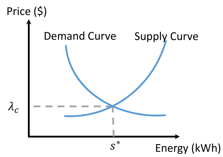
Figure 1: Typical market clearing process

Figure 2: Closed-loop DER dynamics

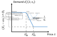
Figure 3: Bidding function in (9)

III Stability Analysis

In this section, we will first define and characterize the market equilibrium. We show that it can be solved from a social welfare optimization problem. Under the assumption of quadratic utility and cost functions, we explicitly characterize (6) by a discrete nonlinear system. We further derive analytical conditions which guarantee the stability of this nonlinear system.

III-A Competitive Equilibrium

The intersection point of the demand curve and the supply curve represents an equilibrium of the market. A competitive equilibrium of the above described electricity market is a tuple $\{\lambda^{*},\,s^{*},\,d_{i}^{*},\forall i\in\mathcal{M}\}$ such that

• $d_{i}^{*}$ maximizes the $i$th consumer’s payoff, that is, it is an optimal solution to the problem (3), for $i\in\mathcal{M}$.

• $s^{*}$ maximize the profit of the supplier, that is, it is an optimal solution to the problem (5).

• $\lambda^{*}$ clears the market, that is, $\sum_{i}d_{i}^{*}(\lambda^{*};x_{i})=c^{-1}(\lambda^{*}).$

From the discussion of the last section, it is clear that given the current state of each DERs, their bids are determined, and the market is cleared at a competitive equilibrium depending on the DERs’ states. It is well known by the welfare theorems that the competitive equilibrium is Pareto efficient and every Pareto efficient allocation is attainable by a competitive equilibrium. The following lemma shows that any competitive equilibrium is efficient, that is, it is an optimal solution to a social welfare maximization problem.

Lemma 1.

The competitive equilibrium $\{\lambda^{*},s^{*},d_{i}^{*},\forall i\in\mathcal{M}\}$ of the electricity market is equivalent to the optimal solution of the following social welfare optimization problem,

$$\begin{array}[]{ll}\underset{d_{i},s}{\mbox{maximize}}&\sum_{i=1}^{N}v_{i}(d_{i},x_{i})-c(s)\\ \mbox{subject to:}&x_{i}^{+}=a_{i}x_{i}+d_{i},\\ &x_{i}^{+}\in\mathcal{X}_{i},\,d_{i}\in\mathcal{D}_{i},\,\forall i\in\mathcal{M}\\ &\sum_{i=1}^{m}d_{i}=s,\end{array}$$ (7)

where the market clearing price $\lambda$ emerges as the Lagrangian dual variable associated with the demand-supply balance constraint (the last equality constraint in (7)).

The proof of the above lemma follows the standard argument by checking that the Karush–Kuhn–Tucker (KKT) conditions of (7) is equivalent to that of (3) and (5), see for example [11].

Note that the social welfare problem (7) has to be solved at each market period after the update of the DERs’ energy states. The DER dynamics (1) with the feedback of the optimal solution $d_{i}^{*},\,\forall i\in\mathcal{M}$ can be viewed as a one-horizon model predictive control (MPC) system, or alternatively, as a system with optimization-based controller [26, 13, 14]. It is well known that such systems could be unstable even when the open loop systems are stable [21]. Although various analytical conditions are proposed in the literature to guarantee the closed-loop stability of the MPC control system [22], they are generally not applicable to the system considered in this paper involving the market clearing process (7). In fact, even the numerical verification of the closed-loop stability (6) with quadratic $v_{i}$ and $c$ can be very challenge [26, 13, 14]. These works usually assume the knowledge of the equilibrium, which is usually the origin. In addition, the numerical conditions proposed there do not scale with the number of the DERs in the market. In the next subsection, we will work with the quadratic utility and cost functions and obtain simple analytical conditions to guarantee the closed-loop system stability and hence the market stability. These conditions will provide valuable insight into market dynamics as well as guidance on the design of the bidding functions.

III-B Closed-loop DER Dynamics

We assume that the utility function $v_{i}$ is a general quadratic function of the power consumption $d_{i}$,

$$v_{i}(d_{i},x_{i})=-\frac{1}{2}q_{i}d_{i}^{2}+(r_{i}x_{i}+c_{i})d_{i},\,\forall i\in\mathcal{M},$$ (8)

where $q_{i}>0$, $r_{i},\,c_{i}\in\mathbb{R}$ are user-specified parameters reflecting their preferences. Such quadratic utility functions have been widely used in coordinating demand-side electric loads via mean-field game approaches, see for example [9] and the references therein. As discussed in the previous section, the bidding function of the $i$th consumer is given by the optimal solution of (3). It can be easily verified that it is the projection of the optimizer of the unconstrained problem onto the constrain set, which is

$$d_{i}^{*}(\lambda)=\text{Proj}_{(\mathcal{X}_{i}-a_{i}x_{i})\cap\mathcal{D}_{i}}\left[\frac{-\lambda+r_{i}x_{i}+c_{i}}{q_{i}}\right],$$ (9)

where the non-emptiness of $(\mathcal{X}_{i}-a_{i}x_{i})\cap\mathcal{D}_{i}$ is guaranteed by the controllability condition (2).

A typical bidding function of the form (9) is depicted in Fig. 3. It contains a linear region in-between the saturated regions. In the figure, there are two threshold prices denoted by $\lambda_{\text{th}}^{1}$ and $\lambda_{\text{th}}^{2}$ . Similar bidding function has also been considered in [19]. Note that the dependence on the load’s state models the time-varying power demand of the consumer.

The cost function is assumed to be

$$c(s)=\frac{1}{2}\beta_{1}s^{2}+\beta_{2}s,$$ (10)

where $\beta_{i}>0$, $i=1,2$. Then the market price which is given by the marginal cost is $\lambda=\beta_{1}s+\beta_{2}$.

Using (8) and (10), we rewrite the social welfare problem (7) in vector form as follows,

$$\begin{array}[]{ll}\underset{d,s}{\mbox{maximize}}&-\frac{1}{2}d^{T}Qd+d^{T}(Rx+c)-\frac{1}{2}\beta_{1}s^{2}-\beta_{2}s\\ \mbox{subject to:}&x^{+}=Ax+d,\,x^{+}\in\mathcal{X},\,d\in\mathcal{D},\\ &{\bf 1}_{m}^{T}d=s,\end{array}$$ (11)

where $d,\,x,\,c\in\mathbb{R}^{m}$ and their $i$th components are $d_{i},\,x_{i},\,c_{i}$, respectively. The diagonal matrices $A,\,Q,\,R$ are generated by the vector $a=\{a_{i}\}$, $q=\{q_{i}\}$, and $r=\{r_{i}\}$ respectively. The state and input constraints are defined by $\mathcal{X}=\Pi_{i=1}^{m}\mathcal{X}_{i}$, $\mathcal{D}=\Pi_{i=1}^{m}\mathcal{D}_{i}$.

Without the inequality constraints, the optimal solution to (11), which we shall refer to as the unconstrained maximizer, can be easily obtained as

$$\hat{d}(x)=\tilde{Q}^{-1}(Rx+\tilde{c}),$$ (12)

where $\tilde{Q}=Q+\beta_{1}{\bf 1}_{m}{\bf 1}_{m}^{T}$ and $\tilde{c}=c-\beta_{2}{\bf 1}_{m}$. The constrained optimal solution can be expressed using $\hat{d}(x)$ conveniently, which is given in the following lemma.

Lemma 2.

The optimal solution to (11) is given by

$$d^{*}(x)=\text{\emph{Proj}}_{(\mathcal{X}-Ax)\cap\mathcal{D}}^{\tilde{Q}}\hat{d}(x).$$ (13)

Proof.

It follows the standard proof as those in for example [9, Lemma 4]. ∎

Note that the feedback policy (13) is nonlinear due to the projection. Overall, the closed-loop system becomes

$$x^{+}=Ax+d^{*}(x).$$ (14)

In particular, it can be shown that (14) is a piecewise linear system [6]. We first observe that the existence of an equilibrium of (14) is simply guaranteed by the controllability condition (2).

Proposition 1.

The closed-loop system (14) has an equilibrium $x^{*}\in\mathcal{X}$ if the controllability condition (2) holds.

Proof.

The equilibria of $x^{+}=Ax+d$ satisfy $(I-A)x=d$. Set $x^{+}=x$ in (11), and replace $s$ with ${\bf 1}_{m}^{T}d={\bf 1}_{m}^{T}(I-A)x$. It can be seen that the convex quadratic programming (possibly degenerated) has a solution if the constraints are non-empty, and the latter can be found to be exactly the controllability condition (2). ∎

Remark 1.

Note that we can further pose conditions to guarantee the uniqueness of the solution to (11) based on the KKT conditions. This is particularly for the degenerated case where the quadratic term is not strongly convex. However, we will not complicate the discussion here, since our stability results in the sequel will guarantee the uniqueness of the equilibrium.

We will investigate the market stability through analyzing the stability of the discrete nonlinear system (14). Specifically, we will find conditions on the utility and the cost functions such that (14) is exponentially stable. In particular, this will guarantee no limit cycle exists. This is desired since the limit cycle corresponds to the oscillation of the power consumption and the high volatility of the market clearing price. Denote by $x^{+}=T(x)$ the discrete time nonlinear dynamics (14). If we can show that $T$ is a contraction mapping on $\mathcal{X}$, then it immediately suggests that there exists a unique equilibrium in $\mathcal{X}$ such that it is exponentially stable. In the case of $a_{i}\in(0,1)$, the globally exponential stability can be concluded in view of the policy (4). Next, we will first consider the single DER case, and then extend the results to the multiple DER case.

III-C Single DER

This scenario arises frequently when an aggregate DER model is obtained by the coordinator to facilitate the power planning, see for example [27, 29, 30, 12]. Such a model represents the aggregate power flexibility of the DER population. It has the same form of (1) but with aggregate power consumption as its input, and has much larger state and input constraint sets. For clarity, we will denote by (scalar) $a$ the system matrix $A$ in this section. First, we have the following characterization of the mapping $T$.

Lemma 3.

Consider the market consisting of one aggregate DER model with $m=1$. Then the nonlinear mapping $T$ of the closed-loop system dynamics (14) is given by

$$\text{\emph{Proj}}_{\mathcal{X}}\left[ax+\emph{Proj}_{\mathcal{D}}\left[\hat{d}(x)\right]\right],$$ (15)

where $\hat{d}(x)$ is defined in (12).

Proof.

First note that for scalar $\tilde{Q}=q+\beta_{1}>0$, it is easy to verify that $\text{Proj}_{(\mathcal{X}-ax)\cap\mathcal{D}}^{\tilde{Q}}$ is equivalent to $\text{Proj}_{(\mathcal{X}-ax)\cap\mathcal{D}}$, i.e., the projection in the $\mathbb{R}^{m}$. Then we need to show that for arbitrary $d$, the following holds.

$$ax+\text{Proj}_{(\mathcal{X}-ax)\cap\mathcal{D}}d=\text{Proj}_{\mathcal{X}}\left[ax+\text{Proj}_{\mathcal{D}}d\right].$$ (16)

If $ax+\text{Proj}_{\mathcal{D}}d\in\mathcal{X}$, then $\text{Proj}_{\mathcal{D}}d\in\mathcal{X}-ax$, and $\text{Proj}_{\mathcal{D}}d=\text{Proj}_{(\mathcal{X}-ax)\cap\mathcal{D}}d$. Hence, the above equality holds. Otherwise, if $ax+\text{Proj}_{\mathcal{D}}d\notin\mathcal{X}$, we assume without loss of generality that $ax+\text{Proj}_{\mathcal{D}}d>\bar{x}$. Then the right hand side of (16) is $\bar{x}$. Since $\text{Proj}_{\mathcal{D}}d>\bar{x}-ax$, we have $\text{Proj}_{(\mathcal{X}-ax)\cap\mathcal{D}}d=\bar{x}-ax,$ and therefore the left hand side is also $\bar{x}$. Thus we proved (16) and also (15). ∎

Under the help of Lemma 3, we have the following theorem for the market stability.

Theorem 1.

Consider the power market consisting of only one DER $(m=1)$ and suppose $a\in(0,1]$, $q,\,\beta_{1}>0$, $r\in\mathbb{R}$. Then the closed-loop system (14) is exponentially stable in $\mathcal{X}$ if the following condition holds

$$\left|a+\frac{r}{q+\beta_{1}}\right|<1.$$ (17)

Proof.

By Lemma 3, the operator $T=\text{Proj}_{\mathcal{\mathcal{X}}}\left[ax+\text{Proj}_{\mathcal{D}}\hat{d}(x)\right]$, where $\hat{d}(x)=rx/(q+\beta_{1})+\tilde{c}$. Without loss of generality, assume $x>y$. We then discuss the two cases $r\geq 0$ and $r<0$.

Case 1: $r\geq 0$. Then $x>y$ implies $\hat{d}(x)\geq\hat{d}(y)$ and it follows that $\text{Proj}_{\mathcal{D}}\hat{d}(x)\geq\text{Proj}_{\mathcal{D}}\hat{d}(y)$, $ax+\text{Proj}_{\mathcal{D}}\hat{d}(x)\geq ay+\text{Proj}_{\mathcal{D}}\hat{d}(y)$, and $T(x)\geq T(y)$. Therefore,

$$\left|T(x)-T(y)\right| =T(x)-T(y)$$

$$\leq a(x-y)+\text{Proj}_{\mathcal{D}}\hat{d}(x)-\text{Proj}_{\mathcal{D}}\hat{d}(y)$$

$$\leq a(x-y)+\hat{d}(x)-\hat{d}(y)$$

$$=(a+\frac{r}{q+\beta_{1}})(x-y)$$

$$<x-y,$$

where the first and second inequalities are by the non-expansive property of the projection operation  [4, Proposition 4.8], and the last inequality is by condition (17).

Case 2: $r<0$. Then $x>y$ implies $\hat{d}(x)<\hat{d}(y)$ and it follows that $\text{Proj}_{\mathcal{D}}\hat{d}(x)\leq\text{Proj}_{\mathcal{D}}\hat{d}(y)$. Therefore,

$$\left|T(x)-T(y)\right| =\left|a(x-y)+\text{Proj}_{\mathcal{D}}\hat{d}(x)-\text{Proj}_{\mathcal{D}}\hat{d}(y)\right|$$

$$\leq\max\Bigl{\{}\text{Proj}_{\mathcal{D}}\hat{d}(y)-\text{Proj}_{\mathcal{D}}\hat{d}(x)+a(y-x),$$

$$\quad a(x-y)\Bigr{\}}$$

$$\leq\max\left\{\hat{d}(y)-\hat{d}(x)+a(y-x),\,a(x-y)\right\}$$

$$=\max\left\{-a-\frac{r}{q+\beta_{1}},\,a\right\}(x-y)$$

$$<x-y,$$

where the second inequality used the non-expansive property of the projection operation, and the last inequality is by condition (17). Combing these two cases, we see that $T$ is a contraction mapping on $\mathcal{X}$. Hence, there exists a unique equilibrium in $\mathcal{X}$ which is exponentially stable. Thus we showed that the system is exponentially stable in $\mathcal{X}$ under condition (17). ∎

Remark 2.

The condition (17) is exact the sufficient and necessary stability condition for the unconstrained closed loop system,

$$x^{+}=Ax+\hat{d}(x).$$

However, it is not necessary for the constrained closed-loop system (14). It is easy to give examples for which the systems do not satisfy (17) but are still globally exponential stable (with equilibrium on the boundary point). Also note that for the energy storage DER with $a=1$ (i.e., no energy dissipation), the coupling coefficient $r$ must be negative.

III-D Multiple DERs

For the case of multiple DERs, the situation is much more complicated than the single DER case. The difficulty mainly stems from the weighted projection $\text{Proj}_{(\mathcal{X}-Ax)\cap\mathcal{D}}^{\tilde{Q}}\hat{d}(x)$ (see (13)). Even though the projection set $(\mathcal{X}-Ax)\cap\mathcal{D}$ is decoupled in $\mathbb{R}^{m}$, the projection of $\hat{d}(x)$ are coupled among each components since $\tilde{Q}\succ 0$ is not diagonal. This reflects the fact that the optimal power consumption of each DER will depend on those of other DERs. Clearly, this is a result of the interaction between DERs through the market coordination. Due to this coupling, we do not have the characterization of $T$ as in (15). However, when the number of DERs is large, they become weakly coupled. In fact, from the unconstrained maximizer $\hat{d}(x)$ we have by the Sherman–Morrison formula [23] that

$$\hat{d}(x) =\tilde{Q}^{-1}(Rx+\tilde{c})$$

$$=\left(I_{m}-\frac{\beta_{1}Q^{-1}{\bf 1}_{m}{\bf 1}_{m}^{T}}{1+\beta_{1}\sum_{i=1}^{m}q_{i}^{-1}}\right)Q^{-1}(Rx+\tilde{c})$$

$$=Q^{-1}Rx-\frac{\beta_{1}Q^{-1}{\bf 1}_{m}}{1+\beta_{1}w_{1}}x_{a}+c_{o},$$

where $x_{a}=\sum_{i\in\mathcal{M}}\frac{r_{i}}{q_{i}}x_{i}$ is the aggregate state, $w_{1}=\sum_{i=1}^{m}q_{i}^{-1}$, and $c_{o}$ is a constant. Moreover, for the $j$th DER, the unconstrained power can be expressed as

$$\hat{d}_{j}(x) =\frac{r_{j}}{q_{j}}x_{j}-\frac{\beta_{1}}{1+\beta_{1}w_{1}}\frac{x_{a}}{q_{j}}+c_{j}$$

$$=\frac{1}{q_{j}}\left(r_{j}x_{j}-\frac{\beta_{1}}{1+\beta_{1}w_{1}}\sum_{i\in\mathcal{M}}\frac{r_{i}}{q_{i}}x_{i}\right)+c_{j},$$

where $c_{j}$ is the $j$th component of $c_{o}$. If $q_{i}^{-1}$ is not diminishing, we have as $m\rightarrow\infty$, $w_{1}\rightarrow\infty$. Hence, the $j$th DER is only affected by the $i$th DER, $\forall i\neq j$, by a diminishing factor of $\frac{\beta_{1}}{1+\beta_{1}w_{1}}\frac{r_{i}}{q_{i}}.$ This motivates us to approximate $\hat{d}(x)$ which couples over all the DERs’ state by a decoupled one, given by,

$$\tilde{d}(x):=\Lambda^{-1}Rx+\tilde{Q}^{-1}\tilde{c},$$ (18)

where $\Lambda$ is diagonal. The diagonal matrix $\Lambda$ will be chosen such that $\epsilon:=\left\|\tilde{Q}^{-1}-\Lambda^{-1}\right\|_{2}$ is sufficiently small. The following lemma gives a approximation matrix $\Lambda$ and derives its approximation error bound.

Lemma 4.

Choose the approximation matrix $\Lambda^{-1}$ as

$$\Lambda^{-1}=Q^{-1}-\frac{1}{2}\frac{\beta_{1}w_{2}}{1+\beta_{1}w_{1}}I_{m},$$ (19)

where $w_{j}=\sum_{i=1}^{m}q_{i}^{-j}$, for $j=1,2$. Then the approximation error is

$$\epsilon\leq\frac{1}{2}\frac{\beta_{1}w_{2}}{1+\beta_{1}w_{1}}.$$

Proof.

Direct calculation yields

$$\left\|\tilde{Q}^{-1}-\Lambda^{-1}\right\|_{2}=\frac{\beta_{1}}{1+\beta_{1}w_{1}}\left\|\frac{1}{2}w_{2}I_{m}-q^{-1}q^{-T}\right\|_{2},$$

where we denote by $q^{-1}$ the column vector $[q_{1}^{-1},...q_{m}^{-1}]^{T}$ and by $q^{-T}$ its transpose. Notice that since $q^{-1}q^{-T}$ is a rank one matrix, it has eigenvalues $\{0,\,w_{2}\}$. It follows immediately that spectral radius of the symmetric matrix $\frac{1}{2}w_{2}I_{m}-q^{-1}q^{-T}$ is $\frac{1}{2}w_{2}$, and hence $\epsilon\leq\frac{1}{2}\frac{\beta_{1}w_{2}}{1+\beta_{1}w_{1}}$. This completes the proof. ∎

Using Lemma 4, we can easily obtain an error bound for the limiting case of an arbitrary number of DERs. The following corollary also reveals that this error bound can be arbitrarily small if all $q_{i}^{\prime}s$ are sufficiently large.

Corollary 1.

Suppose $q_{i}^{-1}$ is not diminishing. Then the approximation error $\epsilon$ is bounded by $\frac{1}{2}\max_{i\in\mathcal{M}}q_{i}^{-1}$.

Proof.

If $q_{i}^{-1}$ is not diminishing, then $w_{1}\rightarrow\infty$ as $m\rightarrow\infty$. It follows from Lemma 4 that

$$\epsilon \leq\frac{1}{2}\frac{\beta_{1}w_{2}}{1+\beta_{1}w_{1}}\leq\frac{1}{2}\frac{\max_{i\in\mathcal{M}}q_{i}^{-1}\beta_{1}w_{1}}{1+\beta_{1}w_{1}},$$

and the right hand side of last inequality goes to $\frac{1}{2}\max_{i\in\mathcal{M}}q_{i}^{-1}$ as $m\rightarrow\infty$. This completes the proof. ∎

It is worth mentioning that in practice, the coefficient $\beta_{1}$ will be relatively very small compare to $q_{i}$, since it denotes the quadratic cost of the total supply cost. Hence, the constant $1$ will dominate the denominator and the error $\epsilon$ will be very small even for a finite number of DERs.

Now the error bounds of using $\tilde{d}(x)$ to approximate $\hat{d}$ can be easily obtained by $\left\|\tilde{d}(x)-\hat{d}(x)\right\|_{2}\leq\epsilon\left\|x\right\|\max r_{i}$ after applying the matrix induced norm inequality. Note that since $x\in(\mathcal{X}-Ax)\cap\mathcal{D}$ is bounded, this error bound is diminishing as $\epsilon\rightarrow 0$ if $r_{i}^{\prime}$s are bounded.

Based on the above results, next we will approximate the constrained maximizer $d^{*}(x)$ in (13) using $\tilde{d}(x)$ in (18). To avoid the cluster of notation, let $\Omega(x)$ denote the projection set $(\mathcal{X}-Ax)\cap\mathcal{D}$. Intuitively, if $\epsilon$ is small, we may approximate $d^{*}(x)$ by $\text{Proj}_{\Omega(x)}^{\Lambda}\tilde{d}(x),$ that is, the projection of $\tilde{d}(x)$ onto $\Omega(x)$ in $\mathcal{H}_{\Lambda}$, where recall that $\tilde{d}(x)$ is the approximation of $\hat{d}(x)$. This approximation can be justified from the KKT conditions corresponding to the projection $d^{*}(x)$. Note that by definition,

$$d^{*}(x)=\arg\min_{z\in\Omega(x)}\left\|z-\tilde{d}(x)\right\|_{\tilde{Q}}.$$ (20)

The KKT conditions for the above minimization problem can be found as,

$$\begin{cases}z=\tilde{d}(x)-\tilde{Q}^{-1}L^{T}\mu,\\ Lz=b(x),\end{cases}$$

where $Lz=b(x)$ are the active inequality constraints in $z\in\Omega(x)$, and $\mu$ the associated Lagrangian multipliers. We see that the optimal projection of $\tilde{d}(x)$ is an affine function of $\mu$ which depends explicitly on $\tilde{Q}^{-1}$. Hence, we will use the following quantity to approximate $d^{*}(x)$,

$$\tilde{d}^{*}:=\text{Proj}_{\Omega(x)}^{\Lambda}\tilde{d}(x)=\arg\min_{z\in\Omega(x)}\left\|z-\tilde{d}(x)\right\|_{\Lambda}.$$ (21)

It is worth mentioning that explicit solutions of the optimal primal and dual solutions $z$ and $\mu$ of (20) can be obtained, see for example [6]. A more thorough analysis based on these explicit solutions will be our future work.

Now based on the approximation (21), we will prove the following sufficient condition to guarantee the market stability. The proof resembles that of the single DER case. The main point is that the approximation $\tilde{d}^{*}$ is totally decoupled among each DERs.

Theorem 2.

Suppose $a_{i}\in(0,1],\,q_{i}>0,\,r_{i}\in\mathbb{R}$. The closed-loop system (14) is exponentially stable if for all $i\in\mathcal{M}$,

$$\left|a_{i}+\phi_{i}r_{i}\right|<1,$$ (22)

where $\phi_{i}$ is the $i$th diagonal element of $\Lambda^{-1}$ in (19), given by

$$\phi_{i}=q_{i}^{-1}-\frac{1}{2}\frac{\beta_{1}w_{2}}{1+\beta_{1}w_{1}},$$

and $w_{j}:=\beta_{1}\sum_{j=1}^{m}q_{j}^{-j}$, for $j=1,2$.

Proof.

We will prove that the mapping $T(x):=Ax+\text{Proj}_{\Omega(x)}^{\Lambda}\tilde{d}(x)$ is contractive.

First note that since $\Lambda$ is diagonal and $\Omega(x)$ is hyper rectangular in $\mathbb{R}^{m}$, it can be easily shown by the definition of the projection that $\text{Proj}_{\Omega(x)}^{\Lambda}\tilde{d}(x)=\text{Proj}_{\Omega(x)}\tilde{d}(x)$. It then follows from the same argument of Lemma 3 component-wisely that

$$Ax+\text{Proj}_{\Omega(x)}\tilde{d}(x)=\text{Proj}_{\mathcal{X}}\left[Ax+\text{Proj}_{\mathcal{D}}\tilde{d}(x)\right].$$ (23)

Using (23) and the non-expansive property of the projection operation [4, Proposition 4.8], we have for arbitrary $x,\,y\in\mathcal{X}$, $x\neq y$,

$$\left\|T(x)-T(y)\right\|_{2} \leq\left\|A(x-y)+\text{Proj}_{\mathcal{D}}\tilde{d}(x)-\text{Proj}_{\mathcal{D}}\tilde{d}(x)\right\|_{2}.$$

Now consider the $i$th element of the vector inside the norm on the right hand side of the above inequality. Similar to the proof of Theorem 1, without loss of generality, we assume $x_{i}>y_{i}$. If $r_{i}\geq 0$, we have by the non-expansiveness of the projection that,

$$0\leq a_{i}(x_{i}-y_{i})+\text{Proj}_{\mathcal{D}_{i}}\tilde{d}_{i}(x)-\text{Proj}_{\mathcal{D}_{i}}\tilde{d}_{i}(y)\\ \leq(a_{i}+\phi_{i}r_{i})(x_{i}-y_{i}),$$ (24)

where $\tilde{d}_{i}(x)$ is the $i$th element of $\tilde{d}(x)$ in (18).

If $r_{i}<0$, then

$$\left|a_{i}(x_{i}-y_{i})+\text{Proj}_{\mathcal{D}_{i}}\tilde{d}(x)-\text{Proj}_{\mathcal{D}_{i}}\tilde{d}(y)\right|\\ \leq\max\Bigl{\{}\text{Proj}_{\mathcal{D}_{i}}\tilde{d}_{i}(y)-\text{Proj}_{\mathcal{D}_{i}}\tilde{d}_{i}(x)+a(y_{i}-x_{i}),\,a_{i}(x_{i}-y_{i})\Bigr{\}}\\ \leq\max\left\{\tilde{d}_{i}(y)-\tilde{d}_{i}(x)+a(y_{i}-x_{i}),\,a_{i}(x_{i}-y_{i})\right\}\\ =\max\left\{-a_{i}-\phi_{i}r_{i},\,a_{i}\right\}(x_{i}-y_{i}),$$ (25)

Combining $(\ref{eq:iterm1})$ and (25), we have

$$\left\|T(x)-T(y)\right\|_{2} \leq\left\|\Xi(x-y)\right\|_{2},$$

where $\Xi$ is a diagonal matrix whose $i$th element is given by

$$\begin{cases}a_{i}+\phi_{i}r_{i},&\text{if $r_{i}\geq 0$,}\\ \max\left\{-a_{i}-\phi_{i}r_{i},\,a_{i}\right\},&\text{if }r_{i}<0.\end{cases}$$

Then by the assumption (22),

$$\left\|T(x)-T(y)\right\|_{2}\leq\left\|\Xi\right\|_{2}\left\|x-y\right\|_{2}<\left\|x-y\right\|_{2},$$

which shows that $T$ is a contraction mapping on $\mathcal{X}$. Hence, the closed-loop system is exponentially stable. Thus it completes the proof. ∎

We see from the above derived condition that if $q_{i}^{-1}$ or $r_{i}$ is sufficiently small, we can always guarantee the stability of the closed-loop system (14). The small $q_{i}^{-1}$ corresponds to a bidding function with a relatively shallower slope.

TABLE I: Parameters for Unstable Market Dynamics

Param.	Value		Param.	Value
	$m=1$	$m=100$		$m=1$	$m=100$
$a_{i}$	$0.95$	U$[0.95,\,0.9]$	$x_{i}(0)$	U$[\underline{x}_{i},\,\bar{x}_{i}]$	U$[\underline{x}_{i},\,\bar{x}_{i}]$
$x_{i}^{r}$	-	U$[350,\,500]$	$q_{i}$	$0.005$	$0.005$
$\underline{x}_{i}$	$2500$	$x_{i}^{r}-200$	$r_{i}$	$-0.1a_{i}$	$-2a_{i}$
$\bar{x}_{i}$	7500	$x_{i}^{r}+200$	$c_{i}$	500	$2x_{i}^{r}$
$\underline{d}_{i}$	$0$	$0$	$\beta_{1}$	$0.04$	$0.008$
$\bar{d}_{i}$	$500$	U$[100,150]$	$\beta_{2}$	$20$	$20$

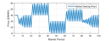
(a) Unstable price response

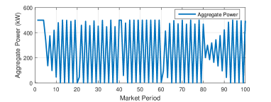
(b) Unstable aggregate power response

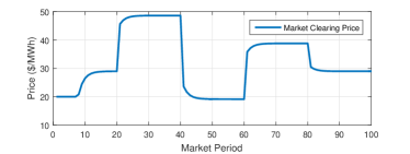
(c) Stable price response

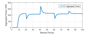
(d) Stable aggregate power response

Figure 4: Single DER market under base price change

(a) Unstable price response

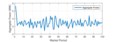
(b) Unstable aggregate power response

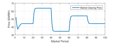
(c) Stable price response

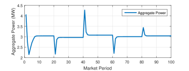
(d) Stable aggregate power response

Figure 5: Multi-DER market under base price change

IV Numerical Examples

In this section, we will present some examples to demonstrate the application of the derived stability conditions. We consider a scenario where the base price changes over time. Note that the base price corresponds to the constant term $\beta_{2}$ in the marginal cost $\lambda=\beta_{1}s+\beta_{2},$ which can be influenced by the external wholesale market price.

IV-A Single DER

We first consider the market consists of only one aggregate DER. The columns below $m=1$ in Table I give the simulation parameters for the unstable market. In the simulation, the base price $\beta_{2}$ is set to $\{20,40,10,30,20\}$ successively every 20 market periods. The price and the aggregate power evolution are depicted in Figs. 54a-4b, respectively. We can see that the resulting market clearing prices and aggregate power keep oscillating. Moreover, the base price as a coordinating signal fails to adjust the aggregate power consumption effectively. Note that in this case, we have $q=0.005$ and the ratio $a+\frac{r}{q+\beta_{1}}=-1.1611$, which violates the condition (17).

If we increase $q$ to $0.2$, then $a+\frac{r}{q+\beta_{1}}=0.5542$ and the condition (17) is satisfied. The resulting market clearing prices and aggregate power become stable in this case, as can be seen from in Figs. 54c-4d.

IV-B Multiple DERs

We next assume that there are $100$ DERs modeled by (1). The parameters for the system dynamics, utility functions, and the cost functions are generated randomly according to the distribution/values in the $m=100$ columns of Table I, where U$[h,l]$ denotes the uniform distribution within the range $[h,l]$, and the variable $x_{i}^{r}$ is used to generate several other variables in the table. The same base price change scenario in the single DER case is simulated where $\beta_{2}$ is set to $\{20,40,10,30,20\}$ successively every 20 market periods. We solve the social welfare problem (11) to obtain the market clearing prices and energy allocation at each market period. As shown in Figs. 54a-4b, both the market clearing prices and the aggregate power are highly volatile and oscillating with large amplitudes. In fact, the condition (22) are violated for all DERs with $a_{i}+\phi_{i}r_{i}\in(-190,-180)$. We next keep the other parameters the same, and choose $q_{i}=1.5$ in order to stabilize the market. With this new $q_{i}$, the condition (22) is satisfied for all DERs, where $a_{i}+\phi_{i}r_{i}$’s are around $-0.09$. The resulted market clearing price and aggregate demand evolution are illustrated in Figs. 54c-4d. We can see that the market converges to an equilibrium very quickly within 10 market periods. It is worth mentioning that one could also change $r_{i}$ to stabilize the market following the stability condition (22). Our extensive simulation shows that condition (22) is a very efficient certification for the market stability under multiple heterogeneous DERs.

V Conclusions and Future Work

This paper investigated the electricity market stability under dynamic DER models. The individual DER was modeled by a scalar linear system with both state and input constraints. Under the assumption of quadratic utility and cost functions, we characterized the competitive equilibrium of the market, and convert the market stability into a discrete nonlinear system stability problem. The stability analysis of such systems is very challenging in general. We derived analytical conditions to guarantee the system stability via a contraction analysis approach. These conditions implied that the market stability can be guaranteed by simply choosing shallower slope or smaller coupling coefficient between individual state and consumption. Numerical examples were provided to demonstrate the application of the stability results.

Our future work includes further investigation of less conservative conditions for the market stability and incorporating the feeder capacity limits into the market model.

References

- [1] “AEP GridSmart Demonstration Project.” [Online]. Available: https://www.smartgrid.gov/document/aep˙ohio˙gridsmart˙demonstration˙project
- [2] F. Alvarado, “The stability of power system markets,” IEEE Trans. Power Syst., vol. 14, no. 2, pp. 505–511, May 1999.
- [3] F. L. Alvarado, “The dynamics of power system markets,” Power Systems Engineering Research Consortium, Tech. Rep., Mar. 1997, pSERC-97-01.
- [4] H. H. Bauschke and P. L. Combettes, Convex Analysis and Monotone Operator Theory in Hilbert Spaces. Springer, 2011.
- [5] A. K. Bejestani, A. Annaswamy, and T. Samad, “A hierarchical transactive control architecture for renewables integration in smart grids: Analytical modeling and stability,” IEEE Trans. Smart Grid, vol. 5, no. 4, pp. 2054–2065, July 2014.
- [6] A. Bemporad, M. Morari, V. Dua, and E. N. Pistikopoulos, “The explicit linear quadratic regulator for constrained systems,” Automatica, vol. 38, no. 1, pp. 3–20, Jan. 2002.
- [7] L. Chen, N. Li, S. H. Low, and J. C. Doyle, “Two market models for demand response in power networks,” in 2010 First IEEE International Conference on Smart Grid Communications, Oct 2010, pp. 397–402.
- [8] J. C. Fuller, K. P. Schneider, and D. Chassin, “Analysis of residential demand response and double-auction markets,” in 2011 IEEE Power and Energy Society General Meeting, July 2011, pp. 1–7.
- [9] S. Grammatico, F. Parise, M. Colombino, and J. Lygeros, “Decentralized convergence to nash equilibria in constrained deterministic mean field control,” IEEE Trans. Automat. Contr., vol. 61, no. 11, pp. 3315–3329, Nov. 2016.
- [10] L. Grüne and J. Pannek, Nonlinear Model Predictive Control. Springer-Verlag London, 2011.
- [11] H. Hao, C. D. Corbin, K. Kalsi, and R. G. Pratt, “Transactive control of commercial buildings for demand response,” IEEE Trans. Power Syst., vol. 32, no. 1, pp. 774–783, 2017.
- [12] H. Hao, B. Sanandaji, K. Poolla, and T. Vincent, “Aggregate flexibility of thermostatically controlled loads,” IEEE Trans. Power Syst., vol. 30, no. 1, pp. 189–198, Jan. 2015.
- [13] W. P. Heath and A. G. Wills, “Zames-falb multipliers for quadratic programming,” in Proceedings of the 44th IEEE Conference on Decision and Control, Dec 2005, pp. 963–968.
- [14] W. P. Heath and G. Li, “Improved multipliers for input-constrained model predictive control,” IFAC Proceedings Volumes, vol. 41, no. 2, pp. 15 160–15 165, 2008.
- [15] T. Hu and Z. Lin, “A complete stability analysis of planar discrete-time linear systems under saturation,” IEEE Transactions on Circuits and Systems I: Fundamental Theory and Applications, vol. 48, no. 6, pp. 710–725, Jun 2001.
- [16] ——, Control Systems with Actuator Saturation. Birkh’́auser Boston, 2001.
- [17] M. Korda and C. N. Jones, “Stability and performance verification of optimization-based controllers,” Automatica, vol. 78, pp. 34–45, April 2017.
- [18] N. Li, L. Chen, and S. H. Low, “Optimal demand response based on utility maximization in power networks,” in 2011 IEEE Power and Energy Society General Meeting, July 2011, pp. 1–8.
- [19] S. Li, W. Zhang, J. Lian, and K. Kalsi, “Market-based coordination of thermostatically controlled loads part I: A mechanism design formulation,” IEEE Trans. Power Syst., vol. 31, no. 2, pp. 1170–1178, 2015.
- [20] D. Liu and A. N. Michel, “Asymptotic stability of discrete-time systems with saturation nonlinearities with applications to digital filters,” IEEE Transactions on Circuits and Systems I: Fundamental Theory and Applications, vol. 39, no. 10, pp. 798–807, Oct 1992.
- [21] J. M. Maciejowski, Predictive control: with constraints. Prentice Hall, 2000.
- [22] D. Mayne, J. Rawlings, C. Rao, and P. Scokaert, “Constrained model predictive control: Stability and optimality,” Automatica, vol. 36, no. 6, pp. 789–814, June 2000.
- [23] C. D. Meyer, Matrix Analysis and Applied Linear Algebra. SIAM, 2000.
- [24] M. S. Nazir and I. A. Hiskens, “Load synchronization and sustained oscillations induced by transactive control,” arXiv:1702.04863. [Online]. Available: https://arxiv.org/pdf/1702.04863.pdf
- [25] J. Nutaro and V. Protopopescu, “The impact of market clearing time and price signal delay on the stability of electric power markets,” IEEE Trans. Power Syst., vol. 24, no. 3, pp. 1337–1345, Aug 2009.
- [26] J. A. Primbs, “The analysis of optimization based controllers,” Automatica, vol. 37, no. 6, pp. 933–938, June 2001.
- [27] M. Roozbehani, M. A. Dahleh, and S. K. Mitter, “Volatility of power grids under real-time pricing,” IEEE Trans. Power Syst., vol. 27, no. 4, pp. 1926–1940, Nov 2012.
- [28] S. E. Widergren, K. Subbarao, J. C. Fuller, D. P. Chassin, A. Somani, M. C. Marinovici, and J. L. Hammerstrom, “AEP Ohio gridSMART Demonstration Project Real-Time Pricing Demonstration Analysis,” Pacific Northwest National Laboratory (PNNL), Tech. Rep., 2014, pNNL Report 23192.
- [29] L. Zhao, H. Hao, and W. Zhang, “Extracting flexibility of heterogeneous deferrable loads via polytopic projection approximation,” in Proc. IEEE Conf. Decision and Control (CDC), 2016.
- [30] L. Zhao, W. Zhang, H. Hao, and K. Kalsi, “A geometric approach to aggregate flexibility modeling of thermostatically controlled loads,” IEEE Trans. Power Syst., To be published.
- [31] D. P. Zhou, M. Roozbehani, M. A. Dahleh, and C. J. Tomlin, “Stability analysis of wholesale electricity markets under dynamic consumption models and real-time pricing,” in 2017 American Control Conference, 2017.