Bayesian Effect Fusion for Categorical Predictors

Abstract

We propose a Bayesian approach to obtain a sparse representation of the effect of a categorical predictor in regression type models. As this effect is captured by a group of level effects, sparsity cannot only be achieved by excluding single irrelevant level effects or the whole group of effects associated to this predictor but also by fusing levels which have essentially the same effect on the response. To achieve this goal, we propose a prior which allows for almost perfect as well as almost zero dependence between level effects a priori. This prior can alternatively be obtained by specifying spike and slab prior distributions on all effect differences associated to this categorical predictor. We show how restricted fusion can be implemented and develop an efficient MCMC method for posterior computation. The performance of the proposed method is investigated on simulated data and we illustrate its application on real data from EU-SILC.

keywords: spike and slab prior, sparsity, nominal and ordinal predictor, regression model, MCMC, Gibbs sampler

1 Introduction

In many applications, especially in medical, social or economic studies, potential covariates collected for a regression analysis are categorical, measured either on an ordinal or on a nominal scale. The usual strategy for modelling the effect of a categorical covariate is to define one level as baseline and to use dummy variables for the effects of the other levels with respect to this baseline. Hence, the effect of a categorical covariate is not captured by a single but by a group of regression effects. Including categorical variables as covariates in regression type models can therefore easily lead to a high-dimensional vector of regression effects. Moreover, as only observations with a specific level contribute information on this level effect, estimated effects of rare levels will be associated with high uncertainty.

Many methods have been proposed to achieve sparsity in regression models by identifying regressors with non-zero effects. Whereas frequentist methods, e.g. the lasso (Tibshirani, 1996) or the elastic net (Zou and Hastie, 2005) rely on penalties, Bayesian variable selection methods are based on the specification of appropriate prior distributions, e.g. shrinkage priors (Park and Casella, 2008; Griffin and Brown, 2010) or spike and slab priors (Mitchell and Beauchamp, 1988; George and McCulloch, 1997; Ishwaran et al., 2005). However, variable selection methods identify single non-zero regression effects and do not take into account the natural grouping of the set of dummy variables capturing the effect of a categorical covariate.

Moreover, for a categorical covariate a sparser representation of its effect cannot only be achieved by restricting some or all of its level effects to zero but also when some of the levels have the same effect. To address this problem, we propose a Bayesian approach to achieve a sparsity by encouraging both shrinkage of non-relevant effects to zero as well as fusion of (almost) identical level effects.

Methods that explicitly address inclusion or exclusion of a whole group of regression coefficients are the group lasso (Yuan and Lin, 2006), the Bayesian group lasso (Raman et al., 2009; Kyung et al., 2010) and the approach of Chipman (1996) who uses spike and slab priors for grouped selection of the set of dummy variables related to a categorical predictor. The recently proposed sparse group lasso (Simon et al., 2013) and Bayesian sparse group selection (Chen et al., 2016) aim at sparsity at the group level as well as within selected groups by selecting non-zero regression effects, but do not consider fusion of effects.

For metric predictors, effect fusion is addressed in Tibshirani et al. (2005) with the fused lasso and in Kyung et al. (2010) with its Bayesian counterpart, the Bayesian fused lasso. Both methods assume some ordering of effects and shrink only effect differences of subsequent effects to zero. Hence, they are not appropriate for nominal predictors where any effect difference should be subject to shrinkage.

Sofar, only a few papers consider effect fusion for nominal predictors. Bondell and Reich (2009) propose a modification of the fused lasso for ANOVA and Gertheiss and Tutz (Gertheiss and Tutz, 2009, 2010; Tutz and Gertheiss, 2016) specify different lasso-type penalties for ordinal and nominal covariates. Recently, Tutz and Berger (2014) propose tree-structured clustering of effects of categorical covariates. In a Bayesian approach, fusion (or merging) of levels of categorical variables is addressed only in Dellaportas and Tarantola (2005). Their goal is to analyse dependence of categorical variables in loglinear models. To search the huge space of models, that can be obtained by collapsing levels of categorical variables, a reversible jump algorithm is employed. This method could be extended to search the space of regression type models where levels of categorical predictors are subject to merging, but we suggest a different approach where Bayesian inference is feasible via a simple Gibbs sampling algorithm.

To allow for effect fusion we specify a joint multivariate Normal prior for all level effects of one covariate with a precision matrix that allows for either almost perfect or low dependence of regression effects. This prior is related to spike and slab prior distributions that have been applied extensively in Bayesian approaches to variable selection. We show that the prior proposed for effect fusion can be derived alternatively by specifying spike and slab prior distributions on all level effects as well as their differences and taking into account their linear dependence. Whereas with the usual variable selection prior regression effects can be classified as (almost) zero, if assigned to the spike, and as non-zero otherwise, the effect fusion prior allows for intrinsic classification of effects as well as of effect differences as negligible or relevant. In contrast to a categorical predictor where typically each pair of level effects will be subject to fusion, for an ordinal predictor the available ordering information can be exploited by restricting fusion to adjacent categories. We show how restriction of effect fusion to specific pairs of effects can be implemented in our framework.

For ease of exposition we will discuss construction of the prior and MCMC inference for a Normal linear regression model with categorical covariates. However, the method we propose can be used in any regression type model with a structured additive predictor, where additionally to effects of categorical covariates further effects, e.g. linear or nonlinear effects of continuous covariates, spatial or random effects are included.

The rest of the paper is organised as follows: in Section 2 we introduce the data model and in Section 3 we describe construction of the prior distribution to encourage a sparse representation of the effect of a categorical predictor. Posterior inference is discussed in Section 4 and Section 5 investigates the performance of the method for simulated data. Application of Bayesian effect fusion is illustrated on a real data example in Section 6 and we conclude with Section 7.

2 Model specification

We consider a standard linear regression model with Normal response $y$ and $p$ categorical covariates where covariate $h$ has $c_{h}+1$ ordered or unordered levels $0,\dots,c_{h}$. To represent the effect of covariate $h$ on the response $y$, we define $0$ as the baseline category and introduce dummy variables, $X_{h,k}$, to capture the effect of level $k$. The regression model is then given as

$$y=\mu+\sum_{h=1}^{p}\sum_{k=1}^{c_{h}}X_{h,k}\beta_{h,k}+\varepsilon,$$ (1)

where $\mu$ is the intercept, $\beta_{h,k}$ is the effect of level $k$ of covariate $h$ (with respect to the baseline category $0$) and $\varepsilon\sim\mathcal{N}\left(0,\sigma^{2}\right)$ is the error term.

For an $(n\times 1)$ response vector ${\mathbf{y}}=(y_{1},\dots,y_{n})^{\prime}$ we write the model as

$${\mathbf{y}}=\mathbf{1}\mu+\sum_{h=1}^{p}{\mathbf{X}}_{h}\boldsymbol{\beta}_{h}+\boldsymbol{\varepsilon},\quad\boldsymbol{\varepsilon}\sim\mathcal{N}\left(\mathbf{0},\sigma^{2}\mathbf{I}\right),$$ (2)

where ${\mathbf{X}}_{h}$ is the $(n\times c_{h})$ design matrix for covariate $h$, $\boldsymbol{\beta}_{h}$ is the $(c_{h}\times 1)$ vector of the corresponding regression effects and $\boldsymbol{\varepsilon}$ the $(n\times 1)$ vector of error terms. $\mathbf{1}$ denotes a vector with elements $1$ and $\mathbf{I}$ the identity matrix.

3 Prior specification

Bayesian model specification is completed by assigning prior distributions to all model parameters. We assume a prior of the structure

$$p(\mu,\boldsymbol{\beta}_{1},\dots,\boldsymbol{\beta}_{p},\sigma^{2})=p(\sigma^{2})p(\mu)\prod_{h=1}^{p}p(\boldsymbol{\beta}_{h}|\tau^{2}_{h},\boldsymbol{\delta}_{h})p(\tau^{2}_{h})p(\boldsymbol{\delta}_{h}),$$

where $\tau^{2}_{h}$ and $\boldsymbol{\delta}_{h}$ denote additional hyperparameters, which are specified below. We assign a flat proper prior $p(\mu)\sim\mathcal{N}\left(0,M_{0}\right)$ to the intercept, and an Inverse Gamma prior $p(\sigma^{2})\sim\mathcal{G}^{-1}\left(s_{0},S_{0}\right)$ to the error variance. In our analyses we use the standard improper prior $p(\sigma^{2})\propto 1/\sigma^{2}$.

To allow for effect fusion we specify the prior on the regression effects $\boldsymbol{\beta}_{h}$ hierarchically as

$$\boldsymbol{\beta}_{h}|\tau^{2}_{h},\boldsymbol{\delta}_{h} \sim\mathcal{N}\left({\mathbf{0}},{\mathbf{B}}_{h0}(\boldsymbol{\delta}_{h},\tau^{2}_{h})\right),$$ (3)

$$\tau_{h}^{2} \sim\mathcal{G}^{-1}(g_{h0},G_{h0}),$$ (4)

with prior covariance matrix of $\boldsymbol{\beta}_{h}$ given as

$${\mathbf{B}}_{h0}(\boldsymbol{\delta}_{h},\tau^{2}_{h})=\gamma_{h}\tau_{h}^{2}{\mathbf{Q}}_{h}^{-1}(\boldsymbol{\delta}_{h}).$$ (5)

Here $\gamma_{h}$ is a fixed constant, $\tau_{h}^{2}$ is a scale parameter and the matrix ${\mathbf{Q}}_{h}(\boldsymbol{\delta}_{h})$ determines the structure of the prior precision matrix of $\boldsymbol{\beta}_{h}$. To encourage effect fusion, we let ${\mathbf{Q}}_{h}(\boldsymbol{\delta}_{h})$ depend on a vector $\boldsymbol{\delta}_{h}$ of binary indicator variables $\delta_{h,kj}$, which are defined for each pair of level effects $\beta_{h,k}$ and $\beta_{h,j}$ subject to fusion. $\delta_{h,kj}=1$ indicates that $\beta_{h,k}$ and $\beta_{h,j}$ differ considerable and hence two regression parameters are needed to capture their respective effects whereas for $\delta_{h,kj}=0$ the effects are almost identical and the two level effects could be fused. To allow also fusion of level effects to $0$, i.e. conventional variable selection, we define $\beta_{h,0}=0$ and include in $\boldsymbol{\delta}_{h}$ also indicators $\delta_{h,k0}$, $k=1,\dots c_{h}$.

The dimension of $\boldsymbol{\delta}_{h}$ and the concrete specification of ${\mathbf{Q}}_{h}(\boldsymbol{\delta}_{h})$ depend on which pairs of effects are subject to fusion. For a nominal covariate typically levels are completely unstructured and hence any pair of effects might be fused. We discuss this case where fusion is unrestricted in Section 3.1.

In contrast, for an ordinal covariate the information on the ordering of levels suggests to restrict fusion to adjacent categories (Gertheiss and Tutz, 2009). Restrictions that preclude direct fusion for specified pairs of effects can easily be implemented in the specification of the prior covariance matrix ${\mathbf{B}}_{h0}(\boldsymbol{\delta}_{h},\tau^{2}_{h})$. We present two different ways to incorporate fusion restrictions in Section 3.2 and discuss the case of an ordinal covariate where fusion is restricted to adjacent categories in more detail.

Marginalized over the indicators $\boldsymbol{\delta}_{h}$, the prior on $\boldsymbol{\beta}_{h}$ is a mixture of multivariate Normal distributions

$$p(\boldsymbol{\beta}_{h}|\tau^{2}_{h})=\sum_{\boldsymbol{\delta}_{h}}p(\boldsymbol{\delta}_{h})f_{\mathcal{N}}\big{(}\boldsymbol{\beta}|{\mathbf{0}},{\mathbf{B}}_{h0}(\boldsymbol{\delta}_{h},\tau_{h}^{2})\big{)},$$

with different component covariance matrices depending on $\boldsymbol{\delta}_{h}$ and mixture weights $p(\boldsymbol{\delta}_{h})$. We discuss specification of the prior on $\boldsymbol{\delta}_{h}$ in Section 3.3 and the choice of the hyperparameters in Section 3.4.

For notational convenience we drop the covariate index $h$ in the rest of this Section.

3.1 Prior for unrestricted effect fusion

To perform unrestricted effect fusion for a categorical covariate with levels $0,\dots,c$, we introduce a binary indicator $\delta_{kj}$ for each pair of effects $0\leq j<k\leq c$. Thus, the vector $\boldsymbol{\delta}$ subsuming all these indicators is of dimension $d\times 1$ where $d={\binom{c+1}{2}}$.

We specify the structure matrix ${\mathbf{Q}}(\boldsymbol{\delta})$ as

$${\mathbf{Q}}(\boldsymbol{\delta})=\begin{pmatrix}\sum_{j\neq 1}\kappa_{1j}&-\kappa_{12}&\dots&-\kappa_{1c}\\ -\kappa_{21}&\sum_{j\neq 2}\kappa_{2j}&\cdots&-\kappa_{2c}\\ \vdots&\vdots&\ddots&\vdots\\ -\kappa_{c1}&-\kappa_{c2}&\dots&\sum_{j\neq c}\kappa_{cj}\end{pmatrix}$$ (6)

with diagonal elements $q_{kk}$ given as

$$q_{kk}=\sum_{j\neq k}\kappa_{kj}=\kappa_{k0}+\dots+\kappa_{k,j-1}+\kappa_{k,j+1}+\kappa_{k,c}\qquad k=1,\dots,c.$$

For $k>j$, $\kappa_{kj}$ is defined as

$$\kappa_{kj}=\delta_{kj}+r(1-\delta_{kj}),$$

and $\kappa_{jk}=\kappa_{kj}$ for $j>k$. The value of $\delta_{kj}$ determines whether $\kappa_{kj}=1$ (for $\delta_{kj}=1$) or $\kappa_{kj}=r$ (for $\delta_{kj}=0$). $r$ is a fixed large number, which we call precision ratio for reasons explained below. Finally, we set $\gamma=c/2$.

We discuss this specification now in more detail. First, as the structure matrix ${\mathbf{Q}}(\boldsymbol{\delta})$ determines the prior precision matrix ${\mathbf{B}}_{0}^{-1}(\boldsymbol{\delta},\tau^{2})$ up to the scale factor $1/(\gamma\tau^{2})$ it has to be symmetric and positive definite. Symmetry of ${\mathbf{Q}}(\boldsymbol{\delta})$ is guaranteed by definition and positive definiteness as

$$\boldsymbol{\beta}^{\prime}{\mathbf{Q}}(\boldsymbol{\delta})\boldsymbol{\beta}=\sum_{k=1}^{c}\beta_{k}^{2}\kappa_{k0}+\sum_{k=2}^{c}\sum_{j=1}^{k-1}(\beta_{k}-\beta_{j})^{2}\kappa_{kj}>0,$$ (7)

if $\boldsymbol{\beta}\neq{\mathbf{0}}$, see Appendix A.1 for a detailed proof.

The diagonal elements $q_{kk}$ determine the prior partial precisions and the off-diagonal elements $q_{kj}$ the prior partial correlations of the level effects:

$$\operatorname{Cor}(\beta_{k},\beta_{j}|\boldsymbol{\beta}_{\setminus kj}) =-\frac{q_{kj}}{\sqrt{q_{jj}q_{kk}}}=\frac{\kappa_{kj}}{\sqrt{q_{jj}q_{kk}}}$$ (8)

$$\operatorname{Prec}(\beta_{k}|\boldsymbol{\beta}_{\setminus k}) =q_{kk}/(\gamma\tau^{2}).$$ (9)

Thus, depending on the value of the binary indicator $\delta_{kj}$, the prior allows for high (if $\delta_{kj}=0$) or low (if $\delta_{kj}=1$) positive prior partial correlation of $\beta_{k}$ and $\beta_{j}$.

The prior partial precision $\operatorname{Prec}(\beta_{k}|\boldsymbol{\beta}_{\setminus k})$ can take one of $c$ different values, depending on the binary indicators involving level $k$. Subsuming these indicators in $\tilde{\boldsymbol{\delta}}_{k}=(\delta_{k0},\dots,\delta_{k,k-1},\delta_{k+1,k},\dots\delta_{c,k})$, the minimum value for $\operatorname{Prec}(\beta_{k}|\boldsymbol{\beta}_{\setminus k})$ results for $\tilde{\boldsymbol{\delta}}_{k}=\mathbf{1}$ as $c/(\gamma\tau^{2})$, and its maximum value, attained for $\tilde{\boldsymbol{\delta}}_{k}=\mathbf{0}$, is $r\cdot c/(\gamma\tau^{2})$. Thus the precision ratio $r$ is the ratio of maximum to minimum prior partial precision. With our choice of $\gamma=c/2$ the partial prior precision ranges from $2/\tau^{2}$ to $r\cdot 2/\tau^{2}$, and does not depend on the number levels $c$.

To illustrate the specification of the structure matrix ${\mathbf{Q}}(\boldsymbol{\delta})$ we consider a covariate with $c=3$ levels where only one of the indicators $\delta_{kj}$, $0\leq j<k\leq c$ has the value $0$ whereas all others are $1$. For a precision ratio of $r=10000$ and $\delta_{10}=0$ the structure matrix is given as

$${\mathbf{Q}}(\boldsymbol{\delta})=\begin{pmatrix}10002&-1&-1\\ -1&3&-1\\ -1&-1&3\end{pmatrix}.$$

The marginal prior on $\beta_{1}$ is concentrated close to zero, thus encouraging fusion to the baseline category. If $\delta_{31}=0$, the structure matrix is

$${\mathbf{Q}}(\boldsymbol{\delta})=\begin{pmatrix}10002&-1&-10000\\ -1&3&-1\\ -10000&-1&10002\end{pmatrix}.$$

Hence, the joint prior on $(\beta_{1},\beta_{3})$ is concentrated close to $\beta_{1}=\beta_{3}$ and encourages fusion of these two effects.

The quadratic form given in equation (7) suggests an interpretation of the effect fusion prior in terms of conditional Normal priors with zero mean and precision proportional to $\kappa_{kj}$ on all effect differences $\theta_{kj}=\beta_{k}-\beta_{j}$, $0\leq j<k\leq c$. For $\delta_{kj}=0$ the prior precision is high with $\kappa_{kj}=r$ and hence the effect difference $\theta_{kj}$ is concentrated around zero, whereas it is more dispersed for $\delta_{kj}=1$ where $\kappa_{kj}=1$. Actually, as we show in Appendix A.2 the effect fusion prior specified above can be derived alternatively by first specifying independent spike and slab priors on all effect differences $\theta_{kj}$, and then correcting for the linear restrictions $\theta_{kj}=\theta_{k0}-\theta_{j0}$. Thus, the proposed prior allows for shrinkage of effect contrasts to zero while taking into account their linear dependence.

As all pairwise effect contrasts $\theta_{kj}$ are taken into account symmetrically, the effect fusion prior is invariant to the choice of the baseline category, see Appendix A.3 for a formal proof. This invariance distinguishes the effect fusion prior from the conventional spike and slab prior used for variable selection, which allows only shrinkage of regression effects $\beta_{k}=\theta_{k0}$, i.e. effect contrasts with respect to the baseline, but not all other effect contrasts $\theta_{kj}$, where $j>0$.

Finally, we note that from a frequentist perspective, the effect fusion prior can be interpreted as an adaptive quadratic penalty with either heavy or slight penalization of effect differences, see equation (7). Similarily, Gertheiss and Tutz (2010) in a frequentist approach use a weighted $L_{1}$ penalty on the effect differences, which has the advantage that effect differences are not only shrunken but can actually be set to zero.

3.2 Prior for restricted effect fusion

We consider now the case where due to available information on the structure of levels fusion is restricted to specific pairs of level effects. A prominent example is an ordinal covariate where the ordering of levels suggests to allow only fusion of subsequent level effects $\beta_{k-1}$ and $\beta_{k}$. A restriction that e.g. $\beta_{k}$ and $\beta_{j}$ should not be fused can be implemented in our prior in two ways: we can either fix the corresponding indicator at $\delta_{kj}=1$ or set the corresponding element in the prior precision matrix ${\mathbf{Q}}(\boldsymbol{\delta})$ to zero. Whereas $q_{kj}=0$ is a hard restriction which implies conditional independence of $\beta_{k}$ and $\beta_{j}$, setting $\delta_{kj}=1$ is a soft restriction which implies that effects $\beta_{k}$ and $\beta_{j}$ are still smoothed to each other.

The implementation of soft restrictions is straightforward, but (hard) conditional independence restrictions require slight modifications in the definition of the structure matrix ${\mathbf{Q}}(\boldsymbol{\delta})$, the vector of indicators $\boldsymbol{\delta}$ and the constant $\gamma$. To specify hard fusion restrictions we introduce a vector $\boldsymbol{\zeta}$ of indicators $\zeta_{kj}$, which are defined for each effect difference $\theta_{kj}$. The elements of $\boldsymbol{\zeta}$ are fixed and indicate whether an effect difference is subject to fusion (for $\zeta_{kj}=1$) or not (for $\zeta_{kj}=0$). Deviating from unrestricted effect fusion considered in Section 3.1, we define a stochastic indicator $\delta_{kj}$ only for those effect differences where $\zeta_{kj}=1$ and hence the dimension of $\boldsymbol{\delta}$ is $d=\sum_{k=1}^{c}\sum_{0\leq j<k}\zeta_{kj}$.

To allow off-diagonal elements of the prior precision to be zero, we set

$$q_{kj}=\begin{cases}-\kappa_{kj}\quad&\text{if }\zeta_{kj}=1\\ \phantom{-}0&\text{if }\zeta_{kj}=0\end{cases}$$

and $q_{jk}=q_{kj}$. Thus, $q_{kj}$ takes the value zero if $\zeta_{kj}=0$ and $-\kappa_{kj}$ otherwise. Accordingly, the diagonal elements are specified as

$$q_{kk}=\begin{cases}\kappa_{k0}-\sum_{k\neq j}q_{kj}\quad&\text{if }\zeta_{k0}=1\\ \phantom{\kappa_{k0}}-\sum_{k\neq j}q_{kj}&\text{if }\zeta_{k0}=0.\end{cases}$$

As noted above, an important special case is an ordinal covariate, where fusion of effects can be restricted to adjacent categories, see Gertheiss and Tutz (2009). We define

$$\zeta_{kj}=\begin{cases}1\qquad&\text{for }j=k-1\\ 0&\text{otherwise}.\end{cases}$$

Thus, the vector of indicators $\boldsymbol{\delta}$ has only $d=c$ elements, $\boldsymbol{\delta}=(\delta_{10},\dots\delta_{c,c-1})$ and ${\mathbf{Q}}(\boldsymbol{\zeta},\boldsymbol{\delta})$ is a tri-diagonal matrix with elements

$${\mathbf{Q}}(\boldsymbol{\zeta},\boldsymbol{\delta})=\begin{pmatrix}\kappa_{10}+\kappa_{21}&-\kappa_{12}&\dots&0&0\\ -\kappa_{21}&\kappa_{21}+\kappa_{32}&\dots&.&0\\ 0&-\kappa_{32}&&\dots&.\\ \vdots&\vdots&\vdots&\ddots&\vdots\\ .&.&\ldots&\kappa_{c-1,c-2}+\kappa_{c,c-1}&-\kappa_{c,c-1}\\ 0&0&\ldots&-\kappa_{c,c-1}&\kappa_{c,c-1}\end{pmatrix}.$$ (10)

In this case, the maximum value of a diagonal element is $q_{kk}=2r$ and therefore we set $\gamma=1$.

It is easy to show that this specification of ${\mathbf{Q}}(\boldsymbol{\zeta},\boldsymbol{\delta})$ corresponds to a random walk prior on the regression effects:

$$\beta_{k}=\beta_{k-1}+\theta_{k},\qquad\theta_{k}\sim\mathcal{N}\left(0,\tau^{2}/\kappa_{k,k-1}\right),$$

with initial value $\beta_{0}=0$. Due to the spike and slab structure, this prior allows for adaptive smoothing, with almost no smoothing for $\delta_{k,k-1}=1$ and pronounced smoothing for $\delta_{k,k-1}=0$.

Another special case of a restricted effect fusion prior is the standard spike and slab prior used for variable selection, which encourages only fusion to the baseline, i.e. shrinkage of $\beta_{k}$ to $\beta_{0}=0$. In our framework the spike and slab prior is recovered with

$$\zeta_{kj}=\begin{cases}1\qquad&\text{for }j=0\\ 0&\text{otherwise}\end{cases}$$

and $\gamma=1$. Therefore the off-diagonal elements of ${\mathbf{Q}}(\boldsymbol{\zeta},\boldsymbol{\delta})$ are zero and $q_{kk}=\kappa_{k0}$.

3.3 Prior on the indicator variables

In variable selection elements of $\boldsymbol{\delta}$ are usually assumed to be conditionally independent a priori with $p(\delta_{kj}=1)=\omega$, where $\omega$ is either fixed or assigned a hyperprior $\omega\sim\mathcal{B}(v_{0},w_{0})$. This would be possible also for the effect fusion prior, but from a computational point of view a more convenient choice is to set

$$p(\boldsymbol{\delta})\propto|{\mathbf{Q}}(\boldsymbol{\delta})|^{-1/2}r^{\sum(1-\delta_{kj})/2}.$$ (11)

Thus, the determinant of ${\mathbf{Q}}(\boldsymbol{\delta})$ cancels out in the joint prior of regression effects and indicators $p(\boldsymbol{\beta},\boldsymbol{\delta}|\tau^{2})$, which results as

$$p(\boldsymbol{\beta},\boldsymbol{\delta}|\tau^{2})=p(\boldsymbol{\beta}|\boldsymbol{\delta},\tau^{2})p(\boldsymbol{\delta})=(\frac{1}{\gamma\tau^{2}})^{c/2}\exp\big{(}-\frac{\boldsymbol{\beta}^{\prime}{\mathbf{Q}}(\boldsymbol{\delta})\boldsymbol{\beta}}{2\gamma\tau^{2}}\big{)}(\sqrt{r})^{\sum(1-\delta_{kj})}.$$ (12)

This prior has attractive features: Firstly, as $p(\boldsymbol{\beta},\boldsymbol{\delta}|\tau^{2})$ can be factorized as

$$p(\boldsymbol{\beta},\boldsymbol{\delta}|\tau^{2}) \propto\prod_{k\neq j}(\sqrt{r})^{1-\delta_{kj}}\exp\Big{(}-\frac{(\beta_{k}-\beta_{j})^{2}}{2\tau^{2}\gamma}\big{(}\delta_{kj}+r(1-\delta_{kj})\big{)}\Big{)}\propto$$ (13)

$$\propto\prod_{k\neq j}p(\theta_{kj},\delta_{kj}|\tau^{2}),$$ (14)

the effect differences $\theta_{kj}$ and indicators $\delta_{kj}$ are jointly independent across all pairs $0\leq j<k\leq c$ conditional on the scale parameter $\tau^{2}$. Secondly, conditioning on the corresponding effect difference $\theta_{kj}$ the conditional prior of the indicator $\delta_{kj}$,

$$p(\delta_{kj}=1|\boldsymbol{\beta},\tau^{2})=\frac{p\big{(}\theta_{kj}|\mathcal{N}\left(0,\gamma\tau^{2}\right)\big{)}}{p\big{(}\theta_{kj}|\mathcal{N}\left(0,\gamma\tau^{2}\right)\big{)}+p\big{(}\theta_{kj}|\mathcal{N}\left(0,\gamma\tau^{2}/r\right)\big{)}},$$ (15)

is identical for all pairs of indices $k,j$ subject to fusion.

The properties of the prior $p(\boldsymbol{\delta})$ given in equation (11) depend on the concrete specification of $\boldsymbol{\delta}$. For the special cases of restricted effect fusion discussed above, fusion of subsequent levels of an ordinal covariate with $\boldsymbol{\delta}=(\delta_{10},\dots\delta_{c,c-1})$ and ${\mathbf{Q}}(\boldsymbol{\delta})$ specified in equation (10), and variable selection with $\boldsymbol{\delta}=(\delta_{10},\dots\delta_{c,0})$ and ${\mathbf{Q}}(\boldsymbol{\delta})=\operatorname{diag}(\kappa_{10},\dots,\kappa_{c0})$, the prior $p(\boldsymbol{\delta})$ is uniform over all $2^{c}$ different values of $\boldsymbol{\delta}$,

$$p(\boldsymbol{\delta})\propto 1,$$

see Appendix A.4 for a formal proof.

In contrast, for a nominal covariate with unrestricted effect fusion $p(\boldsymbol{\delta})$ specified in equation (11) favours sparse models. As ${\mathbf{Q}}(\boldsymbol{\delta})$ has a more complicated structure in this case (see formula (18) in the Appendix), its determinant is not available in closed form for arbitrary $\boldsymbol{\delta}$, but we can compare the full model, where $\boldsymbol{\delta}=\mathbf{1}$ and the null model where $\boldsymbol{\delta}={\mathbf{0}}$ and hence all effects are sampled from the spike component. As $|{\mathbf{Q}}({\mathbf{0}})|=|r{\mathbf{Q}}(\mathbf{1})|$, we get

$$\frac{p(\boldsymbol{\delta}={\mathbf{0}})}{p(\boldsymbol{\delta}=\mathbf{1})}=\frac{|{\mathbf{Q}}(\mathbf{1})|^{1/2}}{|{\mathbf{Q}}({\mathbf{0}})|^{1/2}}\cdot r^{d/2}=r^{-c/2}r^{d/2}=r^{c(c-1)/2}.$$

Thus, a priori the null model is increasingly favoured over the full model with higher number of levels and higher precision ratio.

Figure 1 shows simulations from the marginal prior $p(\boldsymbol{\beta})$ for a categorical regressor with $c=3$ levels (except baseline) for $r=1000$ and $r=10000$. Due to the symmetry of the prior with respect to all level effects only plots for $(\beta_{1},\beta_{2})$ are presented. The prior is concentrated at configurations where all or a subset of the regression effects is zero, or where two effects are equal, $\beta_{j}=\beta_{k}$ and concentration at these configurations increases with the precision ratio $r$.

Figure 1: Simulation from the effect fusion prior: Plot of $(\beta_{1},\beta_{2})$ for $c=3$ and hyperparameters $g_{0}=5$, $G_{0}=2$, $r=1000$ (left) and $r=10000$ (right)

Corresponding plots for simulations from the variable selection prior, where fusion is restricted to $\beta_{k}=0$, and the ordinal fusion prior with fusion restricted to $\beta_{k}=\beta_{k-1}$ are shown in Figure 2. Compared to unrestricted effect fusion, sparsity is much less pronounced in these two priors.

Figure 2: Simulation from the prior: Plot of $(\beta_{1},\beta_{2})$ for $c=3$ and hyperparameters $g_{0}=5$, $G_{0}=20$ and $r=10000$. Left: variable selection prior, right: ordinal fusion prior

3.4 Choice of hyperparameters

To provide a rationale for the choice of the hyperparameters $r,g_{0}$ and $G_{0}$ we focus on the joint marginal prior distribution of one effect difference and the corresponding indicator $0\leq j<k\leq c$. As already noted above, the random variables $(\theta_{kj},\delta_{kj})$ are independent and identically distributed for all pairs of indices $k,j$ conditional on the scale parameter $\tau^{2}$. Marginalized over $\delta_{kj}$ and $\tau^{2}$ the prior an effect difference $\theta_{kj}$ is a spike and slab distribution, where both the spike and the slab are scaled t-distributions with $2g_{0}$ degrees of freedom and scale parameter $\sigma=\sqrt{G_{0}/g_{0}}$ (for $\delta_{kj}=1)$ and $\sigma/\sqrt{r}$ (for $\delta_{kj}=0)$, respectively. For effect fusion we follow the standard choice in variable selection to set $g_{0}=5$ (Fahrmeir et al., 2010; Scheipl et al., 2012) where tails of spike and slab fat enough to avoid MCMC mixing problems when the indicator $\delta_{kj}$ is sampled conditional on $\theta_{kj}$.

Our modelling goal is to allow for fusion of level effects with negligible difference while level effects with relevant difference should be modelled seperately. To avoid misclassification of relevant differences as negligible, which we call false negatives or of negligible effects as relevant, i.e. false positives, the scale parameter $G_{0}$ and the precision ration $r$ could be chosen by specifiying the conditional fusion probability

$$P(\delta_{kj}=0|\theta_{kj})=\frac{1}{1+\frac{t_{2g_{0}}(\frac{\theta_{kj}}{\sigma})}{\sqrt{r}t_{2g_{0}}(\sqrt{r}\frac{\theta_{kj}}{\sigma})}}$$

for two values of $\theta_{kj}.$

Figure 3 shows plots of the fusion probabilities as a function of the effect difference for various values of $r$ and $G_{0}$ with $g_{0}=5$. For fixed $\theta_{kj}$ the fusion probability $P(\delta_{kj}=0|\theta_{kj})$ decreases with $r$ and increases with $G_{0}$ which suggests to choose a large value for $r$ large and a small value for $G_{0}$. However for smaller values of shrinkage effect differences to zero is more pronounced even under the slab, which might hamper detection of small effect differences and hence $G_{0}$ has to be chosen carefully to represent the scale of relevant effects.

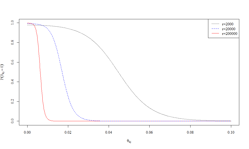
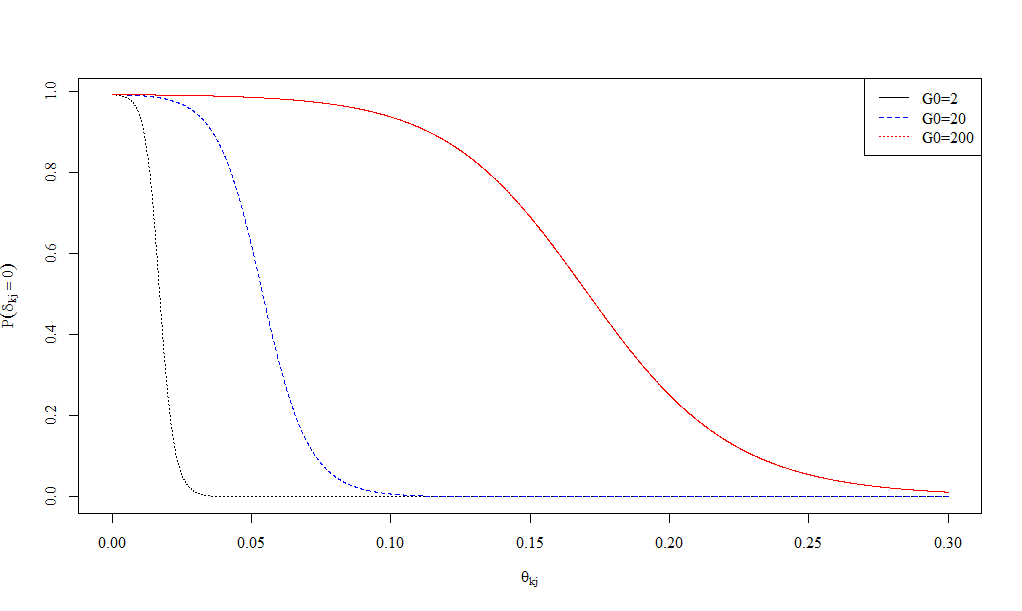
Figure 3: Fusion probabilities for $g_{0}=5$. Left: $G_{0}=2$ and different values of $r$, right: $r=20000$ and different values of $G_{0}$

We will investigate different values for both hyperparameters $G_{0}$ and $r$ in the simulation study in Section 5.3. As suggested by a referee, we investigate also a hyperprior on $G_{0}$, where a convenient choice is an exponential prior $G_{0}\sim\mathcal{E}\left(\lambda\right)$ with mean $\lambda$. We tried also to put a hyperprior on $r$, which did however not prove useful as the additional flexibility resulted in all effect differences being assigned to the spike component.

4 Posterior inference

Our goal is posterior inference for the parameters of linear regression model

$${\mathbf{y}}={\mathbf{X}}\boldsymbol{\beta}+\boldsymbol{\varepsilon},\quad\boldsymbol{\varepsilon}\sim\mathcal{N}\left(0,\sigma^{2}{\mathbf{I}}\right)$$

with prior

$$p(\boldsymbol{\beta},\boldsymbol{\delta},\boldsymbol{\tau}^{2},\sigma^{2})=p(\boldsymbol{\beta}|\boldsymbol{\delta},\boldsymbol{\tau}^{2})p(\boldsymbol{\delta})p(\boldsymbol{\tau}^{2})p(\sigma^{2}).$$

Here the regressor matrix is ${\mathbf{X}}=[\mathbf{1},{\mathbf{X}}_{1},\dots,{\mathbf{X}}_{p}]$ and the vector of regression effects is $\boldsymbol{\beta}=(\mu,\boldsymbol{\beta}_{1}^{\prime},\dots,\boldsymbol{\beta}_{p}^{\prime})^{\prime}$. The vector $\boldsymbol{\delta}=(\boldsymbol{\delta}_{1}^{\prime},\dots,\boldsymbol{\delta}_{p}^{\prime})^{\prime}$ stacks the vectors of binary indicators $\boldsymbol{\delta}_{h}$, $h=1,\dots,p$ and $\boldsymbol{\tau}^{2}=(\tau_{1}^{2},\dots,\tau_{p}^{2})^{\prime}$ subsumes the scale parameters $\tau_{h}^{2}$. The prior for $\boldsymbol{\beta}$ is multivariate Normal, $\boldsymbol{\beta}|\boldsymbol{\delta},\boldsymbol{\tau}^{2}\sim\mathcal{N}\left({\mathbf{0}},{\mathbf{B}}_{0}(\boldsymbol{\delta},\boldsymbol{\tau}^{2})\right)$ with covariance matrix ${\mathbf{B}}_{0}(\boldsymbol{\delta},\boldsymbol{\tau}^{2})$, which is block-diagonal with elements $M_{0}$ (for the intercept) and ${\mathbf{B}}_{h0}(\boldsymbol{\delta}_{h},\tau_{h}^{2})$, $h=1,\dots,p$.

The resulting posterior distribution is proper even for the partial improper prior with $p(\mu,\sigma^{2})\propto\frac{1}{\sigma^{2}}$ under conditions given by a theorem of Sun et al. (2001), see Appendix B.1 for details.

Posterior inference can be accomplished by sampling from the posterior distribution using MCMC methods. For the prior distributions specified above posterior inference for the model parameters is feasible by a Gibbs sampler, where the full conditonals are standard distributions. The sampling scheme is outlined in Section 4.1. Model averaged estimates of the parameters can be obtained as the means of the MCMC draws but often the goal is to select a final model with eventually fused levels. In Section 4.2. we discuss how this model selection problem can be addressed in Bayesian decision theoretic approach by choosing an appropriate loss function.

4.1 MCMC scheme

We initialise MCMC by choosing starting values the error variance $\sigma^{2}$, the indicators $\boldsymbol{\delta}$ and the scale parameters $\boldsymbol{\tau}^{2}$ and compute the prior covariance matrix ${\mathbf{B}}_{0}(\boldsymbol{\delta},\boldsymbol{\tau}^{2})$.

MCMC then iterates the following steps:

1. Sample the regression coefficients $\boldsymbol{\beta}$ from the full conditional Normal posterior $p(\boldsymbol{\beta}|\sigma^{2},\boldsymbol{\delta},\boldsymbol{\tau}^{2},{\mathbf{y}})$.

2. Sample the error variance $\sigma^{2}$ from the full conditional Inverse Gamma distribution $p(\sigma^{2}|\boldsymbol{\beta},\boldsymbol{\delta},\boldsymbol{\tau}^{2},{\mathbf{y}})$.

3. For $h=1,...,p$: Sample the scale parameter $\tau^{2}_{h}$ from the full conditional Inverse Gamma distribution $p(\tau^{2}_{h}|\boldsymbol{\beta},\sigma^{2},\boldsymbol{\delta}_{h})$.

4. For all $h\in\{1,\dots,p\}$ with a hyperprior specified on $G_{h}$: Sample $G_{h}$ from $p(G_{h}|\lambda_{h},\tau_{h}^{2})$

5. For $h=1,\dots,p$: Sample $\boldsymbol{\delta}_{h}$ independently from its full conditional posterior $p(\boldsymbol{\delta}_{h}|\boldsymbol{\beta}_{h},\tau^{2}_{h},\sigma^{2},{\mathbf{y}})$.

6. Update the prior covariance matrix ${\mathbf{B}}_{0}(\boldsymbol{\delta},\boldsymbol{\tau}^{2})$.

Due to the hierarchical structure of the prior, the posterior of $\boldsymbol{\delta}_{h}$ in sampling step (5) depends only on $\boldsymbol{\beta}_{h}$ and $\tau^{2}_{h}$ and as discussed in Section 3.3 elements of $\boldsymbol{\delta}_{h}$ are conditionally independent given $\tau^{2}_{h}$ and $\boldsymbol{\beta}_{h}$. Therefore all binary indicators $\delta_{h,kj}$ can be sampled independently from $p(\delta_{h,kj}=1|\theta_{kj}=\beta_{h,k}-\beta_{h,j},\tau_{h}^{2})$, which is given in equation (15).

Full details of the sampling steps are provided in Appendix B.2. The sampling scheme is implemented in the R package effectFusion (pau-etal:eff).

Compared to posterior inference with a standard Normal prior on the regression effects $\boldsymbol{\beta}$, only steps (3) - (6) have to be added under the effect fusion prior. These steps are fast for nominal covariates that are typical in applications with $2-50$ levels. However, as all pairwise differences are assessed in each sweep of the sampler computation times become prohibitive for covariates with 100 or more levels. For a data set of $n=10000$ observations and one nominal covariate 1000 MCMC iterations take 1.5 seconds for a covariate with $c=20$ levels, but roughly 25 min. for $c=100$ levels on a standard laptop with Intel i7-5600U processor with 2.60 GHz and 16 GB RAM. More details on computation times are given in Appendix B.3.

As already noted above, due to the hierarchical structure of the effect fusion prior the full conditionals of the parameters $\boldsymbol{\delta}_{h},\tau_{h}^{2}$ and $G_{h}$ depend only on the regression effects $\boldsymbol{\beta}_{h}$ and not on the data likelihood. Thus, implementation of effect fusion for categorical covariates is straightforward in any type of regression model with an additively structured linear predictor.

4.2 Model selection

If the goal is to select a final model, e.g. to be used for prediction, a Bayesian decision theoretic approach requires to choose an appropriate loss function. A particularly appealing loss function for effect fusion is a special case Binder’s loss (Binder, 1978) which is used in Lau and Green (2007) for Bayesian model based clustering of observations. It considers pairs of items and penalizes incorrect clustering, which occurs when two items which should not be clustered are assigned to the same cluster or when two items which should be clustered are assigned to different clusters. For effect fusion incorrect clustering corresponds to classifying an effect difference falsely as negative or falsely as positive, respectively.

Binder’s loss is given as

$$\mathcal{L}({\mathbf{z}},{\mathbf{z}}^{*})=\sum_{j\neq k}\big{(}\ell_{1}\mathbf{I}_{\{z_{k}=z_{j}\}}\mathbf{I}_{\{z^{*}_{k}\neq z^{*}_{j}\}}+\ell_{2}\mathbf{I}_{\{z_{k}\neq z_{j}\}}\mathbf{I}_{\{z^{*}_{k}=z^{*}_{j}\}})$$

where ${\mathbf{z}}$ denotes the true and ${\mathbf{z}}^{*}$ the proposed clustering and the constants $\ell_{1}$ and $\ell_{2}$ are misclassification costs. For $\ell_{1}=\ell_{2}$ the expected posterior loss results as

$$\operatorname{E}(\mathcal{L}({\mathbf{z}},{\mathbf{z}}^{*})|{\mathbf{y}})=\sum_{j\neq k}|\mathbf{I}_{\{z^{*}_{k}=z^{*}_{j}\}}-\pi_{kj}|$$ (16)

where $\pi_{kj}=P(z_{k}=z_{j}|{\mathbf{y}})$ denotes the $(k,j)$ element of the posterior similarity matrix, see Fritsch and Ickstadt (2010). The Bayes optimal action, i.e. the clustering which minimizes the expectation of Binder’s loss, can be determined by minimizing

$$\sum_{j\neq k}\mathbf{I}_{\{z^{*}_{k}=z^{*}_{j}\}}(\frac{1}{2}-\pi_{kj}).$$ (17)

For this minimization problem Lau and Green (2007) use an algorithm based on integer programming, which is implemented in the function minbinder (R package mcclust).

We determine the optimal fusion model with respect to the expected posterior Binder loss (16) for each covariate $C_{h}$ seperately and approximate the elements $\pi_{h,kj}$ of the corresponding posterior similarity matrix using $M$ MCMC draws (after burnin) by

$$\hat{\pi}_{h,kj}=\frac{1}{M}\sum_{m=1}^{M}\delta_{h,kj}^{(m)}.$$

Finally, we refit the selected model with dummy-coded regression coefficients for the fused levels under a flat Normal prior $\mathcal{N}\left(0,{\mathbf{I}}B_{0}\right)$.

5 Simulation study

To investigate the performance of the proposed method we conducted a simulation study with a similar set-up as in Gertheiss and Tutz (2010) where we compare results of the finally selected model under the effect fusion prior with respect to parameter estimation, correct effect fusion and predictive performance to various other approaches: penalized regression (Penalty), the Bayesian lasso (BLasso), the Bayesian elastic net (BEN), the group lasso (GLasso), the sparse group lasso (SGL) and the Bayesian Sparse Group Lasso (BSGS). Additionally, we include Bayesian regularization via graph Laplacian (GLap), proposed in Liu et al. (2014), where the prior is also specified directly on the elements of the prior precision matrix, however with the goal to identify conditional independence by shrinking off-diagonal elements to zero. A list of the papers introducing these methods and the related R packages is given in the Appendix C.1. For comparison we also fit the full model (Full) with separate dummy variables for each level and the true model (True), i.e. the model where correct fusion is assumed to be known.

5.1 Simulation set-up

We generated 100 data sets with $n=500$ observations from the Gaussian linear regression model (2) with intercept $\mu=1$, a standard Normal error $\varepsilon\sim\mathcal{N}\left(0,1\right)$ and fixed design matrix ${\mathbf{X}}$. We use four ordinal and four nominal predictors, where two regressors have eight and two have four categories for each type of covariate (ordinal and nominal). Regression effects are set to $\boldsymbol{\beta}_{1}=(0,1,1,2,2,4,4)$ and $\boldsymbol{\beta}_{3}=(0,-2,-2)$ for the ordinal, to $\boldsymbol{\beta}_{5}=(0,1,1,1,1,-2,-2)$ and $\boldsymbol{\beta}_{7}=(0,2,2)$ for the nominal covariates, and $\boldsymbol{\beta}_{h}={\mathbf{0}}$ for $h=2,4,6,8$. Levels of the predictors are generated with probabilities $(0.1,0.1,0.2,0.05,0.2,0.1,0.2,0.05)$ and $(0.1,0.4,0.2,0.3)$ for regressors with eight and four levels, respectively.

To perform effect fusion, we specify a Normal prior with variance $B_{0}=10000$ on the intercept and the improper prior $p(\sigma^{2})\propto 1/\sigma^{2}$ (which corresponds to an Inverse Gamma distribution with parameters $s_{0}=S_{0}=0$) on the error variance $\sigma^{2}$. For each covariate $h$, the hyperparameters are set to $G_{h0}=20$ and $r=20000$, but we investigate also various other values for both parameters and an exponential hyperprior on $G_{h0}$ with $\lambda=\operatorname{E}(G_{h0})=2$ in Section 5.3.

MCMC is run for 10000 iterations after burnin of 5000 to perform model selection for each data set. Models Full and True and the refit of the selected model are estimated under a flat Normal prior $\mathcal{N}\left(0,{\mathbf{I}}B_{0}\right)$ on the regression coefficients where $B_{0}=10000$ with MCMC run for 3000 iterations (after a burnin of 1000). The tuning parameters of the frequentist methods Penalty and GLasso are selected automatically via cross-validation in the corresponding R packages. For SGL we choose the penalty parameter via cross-validation in the range from $0.00005$ to $0.05$. For the Bayesian methods, we use the default prior parameter settings in the code (for GLap) and the R packages monomvn and EBglmNet and estimate the regression coefficients by the posterior means. For BSGS which is tailored to sparse group selection of numeric regressors in a model with no intercept the recommendation in Lee and Chen (2015) to demean the response is not useful in our setting and hence we set the prior inclusion probability for the intercept to 0.99 (which due to implementation specifics resulted in a higher posterior inclusion probability than a value of 1) and used the default value of 0.5 for all other covariates.

5.2 Simulation results

We first compare the different methods with respect to estimation of the regression effects. Figure 4 shows boxplots of the mean squared estimation error (MSE), which is defined for data set $i$ and covariate $h$ as

$$MSE_{h}^{(i)}=\frac{1}{c_{h}}\sum_{k=1}^{c_{h}}(\hat{\beta}_{h,k}^{(i)}-\beta_{h,k})^{2}.$$

No method outperforms the others consistently in all data sets for all covariates. The mean MSE (averaged over all 100 data sets) is lower for Bayesian effect fusion (Effect Fusion) than in the model Full and only slightly higher than in the model True for all covariates. Effect Fusion outperforms all other methods with respect to the mean MSE for the ordinal covariates 1 and 3 and for all nominal covariates (5 - 8). However, due to high MSEs in some data sets it is outperformed by BLasso and BSGS for the ordinal covariates 2 and 4 (both with no effect on the response) and for covariate 4 also by BEN. Though overall performance of Effect Fusion is very good, for single data sets the MSE can be even higher than for the model Full. This occurs when levels with actually different effects are fused, e.g. for some of the 8 levels of the nominal covariate 5.

The frequentist method for effect fusion, Penalty, which uses a global penalty parameter across all covariates yields a lower MSE than the model Full for covariates with no effect and for ordinal covariates, but only small improvements for nominal covariates.

BLasso which aims at shrinkage of effects to zero performs very well for covariates with no effect but also good for the other covariates 1, 3, 5 and 7. The performance of BEN is similar, however slightly worse than that of BLasso for all covariates. As expected, GLasso which aims at sparsity at the group level performs well for covariates with no effect but MSEs are similar to those of the model Full for covariates with non-zero effects. GLap which is designed for a different goal yields small improvements for covariates with no effect compared to the model Full and performs similar for covariates with non-zero effects. Finally, both SGL and BSGS, which aim at sparsity at the group level as well as within groups of effects outperform Full for covariates with no effect and to a smaller extent also for the nominal covariates 5 and 7, where some level effects are zero. However, SGL performs worse then Full for covariates 1 and 3, where the ordinal structure is not taken into account. BSGS performs almost as good as True and similar to Effect Fusion (slightly better for covariates 2 and 4, slightly worse for covariates 6 and 8) for covariates with no effects. For nominal and ordinal covariates with non-zero effects it is outperformed by Effect Fusion but similar as the two other Bayesian methods BLasso and BEN.

Also model averaged estimates (not shown in Figure 4), which are obtained as posterior mean estimates from the first MCMC run under the effect fusion prior, perform very well with respect to MSE.

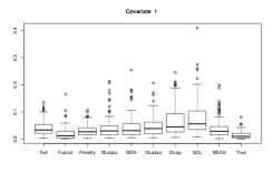
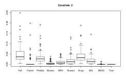
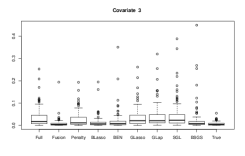
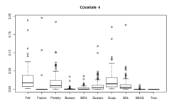
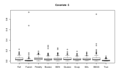
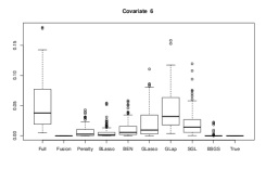
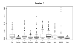
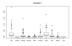
Figure 4: Simulation study: MSE for ordinal (Covariates 1 - 4) and nominal covariates (Covariates 5 - 8) in 100 simulated data sets. Covariates 2, 4, 6, and 8 (right panel) have no effect on the response.

To evaluate the predictive performance of Bayesian effect fusion, we generate a new sample of $n^{*}=500$ observations $z_{j},\;j=1,\dots,n^{*}$ from the linear regression model (2) with fixed regressors $\tilde{{\mathbf{x}}}_{j}$ and the same parameters as in the simulated data sets. Predictions for these new observations are computed using the estimates from each of the original data sets as $\hat{z}_{j}^{(i)}=\tilde{\mathbf{x}}_{j}\hat{\boldsymbol{\beta}}^{(i)},i=1,\dots,100$.

The mean squared prediction errors (MSPE) defined for each data set as

$$\text{MSPE}^{(i)}=\frac{1}{n^{*}}\sum_{j=1}^{n^{*}}(z_{j}-\hat{z}_{j}^{(i)})^{2},\quad i=1,\dots,100$$

are shown in Figure 5. The predictive performance of Bayesian effect fusion is almost as good as for the model True with correctly fused effects, and is considerably better for than all competing methods in most data sets. The Bayesian methods BLasso and BSGS perform similar with respect to the mean MPSE (averaged over 100 data sets) and slightly better than Penalty, BEN and GLasso. Finally, MSPEs for SGL and GLap are similar to those of model Full.

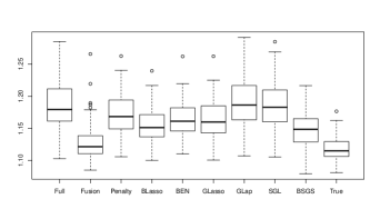
Figure 5: Simulation study: MSPE of 500 new observations. Predictions are based on the estimates from 100 simulated data sets.

Finally, to evaluate and compare the performance of the methods with respect to model selection, we report for each covariate the true positive rate (TPR), the true negative rate (TNR), the positive predictive value (PPV) and the negative predictive value (NPV), see Appendix C.2 for detailed definitions. If fusion is completely correct, all four values are equal to 100% but TPR and PPV are not defined for covariates where all effects are zero. For the effect fusion prior we perform model selection as described in Section 4.2, for the other methods we consider two level effects as identical if the posterior mean of their difference is smaller or equal to 0.01. Tables 1 and 2 report the averages of these statistics in the 100 simulated data sets for each covariate seperately. Bayesian effect fusion which clearly outperforms all other methods with respect to identifying categories with the same effect with averaged TNR higher than 95% for all covariates. This comes at the cost of occasionally missing a non-zero effect difference and hence an average TPR slightly lower than 100%.

Covariate	Method	TPR	TNR	PPV	NPV
1	Fusion	99.7	95.3	95.3	99.8
	Penalty	100	18.8	48.8	100
	BLasso	100	6.8	44.8	100
	BEN	100	19.2	48.5	100
	GLasso	100	2.2	43.5	100
	GLap	100	2.5	43.6	100
	SGL	100	8.7	45.4	100
	BSGS	100	12.5	46.5	100
2	Fusion	-	98.3	-	100
	Penalty	-	21.3	-	100
	BLasso	-	24.1	-	100
	BEN	-	53.9	-	100
	GLasso	-	21.7	-	100
	GLap	-	2.7	-	100
	SGL	-	17.3	-	100
	BSGS	-	83.7	-	100
3	Fusion	100	99.0	99.3	100
	Penalty	100	24.5	44.8	100
	BLasso	100	25.0	43.7	100
	BEN	100	46.5	52.5	100
	GLasso	100	10.5	36.8	100
	GLap	100	6.5	35.5	100
	SGL	100	17.5	39.5	100
	BSGS	100	27.5	43.8	100
4	Fusion	-	99.0	-	100
	Penalty	-	21.3	-	100
	BLasso	-	48.3	-	100
	BEN	-	61.3	-	100
	GLasso	-	34.0	-	100
	GLap	-	7.3	-	100
	SGL	-	18.0		100
	BSGS	-	81.7	-	100

Table 1: Simulation study: Model selection results for ordinal covariates. TPR, TNR, PPV and NPV are averaged over 100 data sets.

Covariate	Method	TPR	TNR	PPV	NPV
5	Fusion	99.1	98.8	99.5	98.5
	Penalty	100	17.2	75.3	100
	BLasso	100	6.8	72.9	100
	BEN	99.9	12.0	74.0	99.5
	GLasso	100	4.2	72.3	100
	GLap	100	4.0	72.3	100
	SGL	100	7.1	73.0	100
	BSGS	100	7.6	73.1	100
6	Fusion	-	100	-	100
	Penalty	-	51.4	-	100
	BLasso	-	27.5	-	100
	BEN	-	54.5	-	100
	GLasso	-	21.3	-	100
	GLap	-	3.9	-	100
	SGL	-	19.5		100
	BSGS	-	84.2	-	100
7	Fusion	100	99.5	99.8	100
	Penalty	100	17.5	71.6	100
	BLasso	100	22.5	72.7	100
	BEN	100	43.0	78.3	100
	GLasso	100	5.5	68.1	100
	GLap	100	4.5	67.9	100
	SGL	100	15.0	70.7	100
	BSGS	100	32.0	75.6	100
8	Fusion	-	100	-	100
	Penalty	-	27.5	-	100
	BLasso	-	47.8	-	100
	BEN	-	70.2	-	100
	GLasso	-	35.3	-	100
	GLap	-	4.7	-	100
	SGL	-	19.3		100
	BSGS	-	85.3	-	100

Table 2: Simulation study: Model selection results for nominal covariates. TPR, TNR, PPV and NPV are averaged over 100 data sets.

5.3 Influence of hyperparameters

In this section, we investigate the sensitivity of model selection under the effect fusion prior with respect to the hyperparameters. While false positives result in a loss of estimation efficiency, false negatives will yield biased effect estimates and poor predictive performance, and hence the goal is to avoid false negatives while keeping false positives at a moderate level. We report false negative rates, $\text{FNR}=1-\text{TPR}$ and false positive rates $\text{FPR}=1-\text{TNR}$ for various values of $G_{0}$ and fixed $r=20000$ in Table 3 and for various values of $r$ and fixed $G_{0}=20$ in Table 4. Results in Table 3 indicate that increasing $G_{0}$ from $0.2$ to $200$ has little effect on FNR but yields lower FPR for ordinal predictors (covariates 1 – 4), and has little effect on FPR but leads to higher FNR for nominal predictors (covariates 5 – 8). We conclude that for nominal predictors $G_{0}=2$ is a good choice which allows to detect also small effect differences whereas for ordinal predictors we suggest to choose a larger value for $G_{0}$, e.g. $G_{0}=20$. An exponential hyperprior with $\operatorname{E}(G_{0})=2$ performs similar to a fixed value of $G_{0}=2$ with slightly lower FNR and FPR for nominal covariates but higher FPR for ordinal covariates.

Table 4 reports FNR and FPR for values of the precision ratio $r$ from $2\cdot 10^{2}$ to $2\cdot 10^{5}$. Whereas for ordinal predictors FNR and FPR change only little with $r$, for nominal covariates low values of $r$ encourage too much fusion of effects and hence result in a high FNR. Both FNR and FPR are small for $r=2\cdot 10^{4}$ and $r=2\cdot 10^{5}$. As MCMC mixing is adequate for both values, we suggest to choose $r$ in this range.

	$G_{0}=0.2$		$G_{0}=2$		$G_{0}=20$		$G_{0}=200$		$G_{0}\sim\mathcal{E}\left(2\right)$
h	$FNR_{h}$	$FPR_{h}$	$FNR_{h}$	$FPR_{h}$	$FNR_{h}$	$FPR_{h}$	$FNR_{h}$	$FPR_{h}$	$FNR_{h}$	$FPR_{h}$
1	0.0	13.0	0.3	10.5	0.3	4.7	0.7	1.7	0.3	9.0
2	-	18.9	-	7.4	-	1.7	-	0.3	-	11.7
3	0.0	11.0	0.0	7.5	0.0	1.0	0.0	0.5	0.0	5.0
4	-	14.3	-	5.0	-	1.0	-	0.3	-	8.7
5	0.4	1.2	0.7	1.0	0.9	1.2	81.0	0.0	0.5	0.9
6	-	0.0	-	0.0	-	0.0	-	0.0	-	0.0
7	0.0	3.0	0.0	2.0	0.0	0.5	0.0	0.0	0.0	1.5
8	-	0.0	-	0.0	-	0.0	-	0.0	-	0.0

Table 3: Simulation study: Model selection results for $r=20,000$ and various values of $G_{0}$

	$r=200$		$r=2,000$		$r=20,000$		$r=200,000$
h	$FNR_{h}$	$FPR_{h}$	$FNR_{h}$	$FPR_{h}$	$FNR_{h}$	$FPR_{h}$	$FNR_{h}$	$FPR_{h}$
1	0.3	2.7	0.3	4.2	0.3	4.7	0.3	3.0
2	-	0.9	-	1.4	-	1.7	-	1.7
3	0.0	0.5	0.0	1.5	0.0	1.0	0.0	2.0
4	-	0.3	-	0.3	-	1.0	-	1.7
5	100.0	0.0	92.0	0.0	0.9	1.2	0.8	1.9
6	-	0.0	-	0.0	-	0.0	-	0.6
7	0.0	0.0	0.0	0.0	0.0	0.5	0.0	0.5
8	-	0.0	-	0.0	-	0.0	-	0.0

Table 4: Simulation study: Model selection results for $G_{0}=20$ and various values of $r$

6 Real data example

As an illustration of Bayesian effect fusion on real data, we model contributions to private retirement pension in Austria. The data were collected in the European household survey EU-SILC (SILC = Survey on Income and Living Conditions) 2010 in Austria. We use a linear regression model to analyse the effects of socio-demographic variables on the (log-transformed) annual contributions to private retirement pensions. As potential regressors we consider gender (binary, 1=female/0=male), age group (ordinal with eleven levels), child in household (binary, 1=yes/0=no), income class (in quartiles of the total data set, i.e. ordinal with four levels), federal state of residence in Austria (nominal with nine levels), highest attained level of education (nominal with ten levels) and employment status (nominal with four levels). We restrict the analysis to observations without missing values in either regressors or response and a minimum annual contribution of EUR 100. Hence, the final data set used for our analysis comprises data of 3077 persons.

We standardised the response and fit a regression model including all potential covariates. Results reported in Table 5 indicate that several levels of covariate education have a similar effect and most level effects of federal state are close to zero, which suggests that a sparser model might be adequate for these data.

	Full model	95%		Selected model	95%
	Posterior mean	HPD interval		Posterior mean	HPD interval
Intercept	-1.15	(-1.38 – -0.91)		-1.10	(-1.31 – -0.90)
Age
20-25	0.20	(-0.03 – 0.42)	}20.5mm	0.33	(0.14 – 0.52)
25-30	0.36	(0.15 – 0.57)
30-35	0.60	(0.40 – 0.80)		0.65	(0.45 – 0.86)
35-40	0.74	(0.53 – 0.95)	}20.5mm
40-45	0.80	(0.60 – 1.00)		0.82	(0.62 – 1.01)
45-50	0.90	(0.70 – 1.10)		0.93	(0.74 – 1.13)
50-55	1.01	(0.80 – 1.23)	}40.5mm
55-60	1.06	(0.81 – 1.30)
60-65	1.23	(0.83 – 1.62)		1.05	(0.85 – 1.24)
$>$ 65	0.67	(0.14 – 1.22)
Female	-0.24	(-0.32 – -0.17)		-0.25	(-0.31 – -0.18)
Child	0.00	(-0.07 – 0.07)		-	-
Income
2nd quartile	0.20	(0.07 – 0.32)	}20.5mm
3rd quartile	0.25	(0.13 – 0.37)		0.23	(0.12 – 0.35)
4th quartile	0.52	(0.40 – 0.64)		0.54	(0.42 – 0.66)
Federal State
Carinthia	-0.16	(-0.30 – -0.01)		-	-
Lower Austria	0.06	(-0.03 – 0.16)		-	-
Burgenland	-0.03	(-0.21 – 0.15)		-	-
Salzburg	0.15	(0.01 – 0.30)		-	-
Styria	0.01	(-0.10 – 0.13)		-	-
Tyrol	0.08	(-0.06 – 0.20)		-	-
Vorarlberg	0.02	(-0.15 – 0.19)		-	-
Vienna	0.00	(-0.11 – 0.10)		-	-
Education
Apprenticeship, trainee	0.09	(-0.04 – 0.23)		0.00	-
Master craftman’s diploma	0.24	(0.06 – 0.43)	}100.5mm
Nurse’s training school	0.22	(-0.04 – 0.47)
Other vocational school
(medium level)	0.26	(0.11 – 0.42)
Academic secondary school
(upper level)	0.22	(0.05 – 0.37)		0.21	(0.14 – 0.28)
College for higher vocational
education	0.28	(0.12 – 0.43)
Vocational school for apprentices	0.29	(0.06 – 0.51)
University, academy: first degree	0.35	(0.20 – 0.49)
University: doctoral studies	1.12	(0.85 – 1.37)		1.03	(0.80 – 1.26)
Employment status
Unemployed	-0.10	(-0.34 – 0.12)		-	-
Retired	-0.15	(-0.37 – 0.07)		-	-
Not-working
(other reason)	0.01	(-0.11 – 0.14)		-	-

Table 5: EU-SILC data: Posterior means and 95% HPD intervals of regression effects in the full and in the selected model.

To specify the effect fusion prior, we chose the hyperparameters with $r=50000$, $g_{h0}=5$, $G_{h0}=2$ for nominal and $G_{h0}=20$ for ordinal predictors and used the improper prior $p(\sigma^{2})=\frac{1}{\sigma^{2}}$. MCMC was run for 50000 iterations after a burn-in of 30000 with the first 500 draws of the burnin drawn from the unrestricted model where all elements of $\boldsymbol{\delta}$ are 1. The median of the integrated autocorrelation times over all regression effects was 11.9 (range 1 - 104) and integrated autocorrelation times were lower than 30 for effects of all covariates except age. We ran several chains from different starting values which yielded essentially the same results.

Figure 6 shows the estimated posterior means of the pairwise fusion probabilities $1-\hat{\pi}_{h,kk-1}$ for the ordinal covariate age group. The estimated fusion probability is higher than 0.5 (dotted line) for five levels, which indicates that age categories could be fused as follows: categories $20-25$ and $25-30$ to $20-30$, categories $35-40$ and $40-45$ to $35-45$ and finally the three categories $50-55$, $55-60$ and $60-65$ to a new category $50-65$.

For a nominal covariate we suggest to visualize the pairwise fusion probabilities in a heatmap. Figure 7 shows the corresponding heatmap for the covariate education, where all pairwise fusion probabilities are displayed. Darker colours indicate higher fusion probabilities and values in the diagonal (which represent fusion probability of a category with itself) are always one. Obviously, only three levels are required to capture the effect of education (secondary school and apprenticeship; doctoral degree; all remaining levels) and thus the number of effects to be estimated reduces from nine to two.

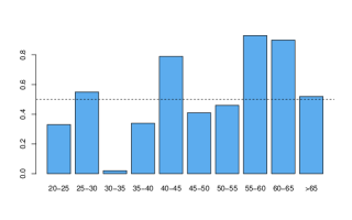
Figure 6: EU-SILC data, covariate age group: estimated probabilities for fusion with preceding level

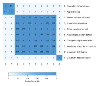
Figure 7: EU-SILC data, covariate education: Estimated pairwise fusion probabilities of level effects (baseline: category 0). Darker colours indicate higher fusion probabilities.

Based on the estimated pairwise fusion probabilities we select the final model for all covariates as described in Section 4.2. Covariates child, federal state and employment status are completely excluded from the model, whereas some of the levels are fused for covariates age group, income class and education. Thus, the final model has only 11 regression effects compared to 35 in the full model. Results from a refit of the selected model using flat priors are reported in the right panel of Table 5. The posterior mean of the error variance, $\hat{\sigma}^{2}=0.829$, is almost identical to that of the full model, where $\hat{\sigma}^{2}=0.826$.

7 Conclusion

In this paper, we present a method that allows for sparse modelling of the effects of categorical covariates in Bayesian regression models. Sparsity is achieved by excluding irrelevant predictors and by fusing levels which have essentially the same effect on the response. To encourage effect fusion, we propose a finite mixture of Normal prior distributions with component specific precision matrices, that allow for almost perfect or almost zero partial dependence of level effects. Alternatively, this prior can be derived by specifying spike and slab prior distributions on all level effect contrasts associated with one covariate and taking the linear restrictions among them into account. The structure of prior easily allows to incorporate prior information that restricts direct fusion to specific pairs of level effects. This property is of particular interest for ordinal covariates where fusion usually will be restricted to effects of subsequent levels.

Posterior inference for all model parameters is straightforward using MCMC methods. To select the final model we suggest to determine the clustering of level effects which minimizes Binder’s loss based on the estimated posterior means of the pairwise fusion probabilities. Simulation results show that the proposed method automatically excludes irrelevant predictors and outperforms competing methods in terms of correct model selection, coefficient estimation as well as predictive performance.

The proposed method for Bayesian effect fusion is not restricted to linear regression models with categorical predictors but can be applied in more general regression type models e.g. generalised linear models, with a structured additive predictor that also contains other types of effects, e.g. nonlinear or spatial effects. Implementation of effect fusion requires little adaption of an MCMC scheme for posterior sampling of any Bayesian regression type model with a Gaussian prior on the regression effects as only two Gibbs sampling steps and the update of the structure matrix have to be added in each MCMC sweep.

A certain drawback of the method is that all pairwise effect differences have to be determined and classified in each MCMC sampling step to construct the prior covariance matrix and hence the computational effort can be prohibitive for nominal covariates with a large number of levels. If we consider each combination of spike and slab distribution on effect differences as a different model, then for a nominal covariate with $c+1$ levels the procedure searches a space of $2^{c(c+1)/2}$ different models. This number is much larger than the number of possible clusterings, which is given by the Bell number $B(c+1)$ of order $c$. A search in the model space of possible clusterings could be performed by employing a reversible jump MCMC algorithm as in Dellaportas and Tarantola (2005). Another option to determine a model with eventually fused level effects was recently proposed in mal-etal:eff. The authors use model-based clustering methods and specify a finite mixture prior with many spiky components on the level effects. The prior on the mixture weights encourages empty components and thus some level effects will be assigned to the same mixture component. Due to the spikyness of the components, almost identical effects are assigned to the same component which suggests to fuse effects according to the clustering solution. This approach works well for nominal covariates but does not easily allow incorporation of fusion restrictions.

Acknowledgement: This work was financially supported by the Austrian Science Fund (FWF) via the research project number P25850 ’Sparse Bayesian modelling for categorical predictors’.

Appendix A Properties of the effect fusion prior

A.1 Properties of the structure matrix

For simplicity of notation, we drop dependence of the structure matrix ${\mathbf{Q}}(\boldsymbol{\delta})$ on $\boldsymbol{\delta}$ in the following. ${\mathbf{Q}}$ is symmetric by definition. To show its positive definiteness we consider the quadratic form ${\mathbf{x}}^{\prime}{\mathbf{Q}}{\mathbf{x}}$ where ${\mathbf{x}}$ is a non-zero vector of dimension $c$.

Obviously, we have

$${\mathbf{x}}^{\prime}{\mathbf{Q}}{\mathbf{x}} =\sum_{k=1}^{c}\sum_{j=1}^{c}x_{k}x_{j}q_{kj}=$$

$$=\sum_{k=1}^{c}x_{k}^{2}\Big{(}\sum_{j\neq k}\kappa_{kj}\Big{)}-\sum_{k=1}^{c}\sum\limits_{\begin{subarray}{c}j=1\\ j\neq k\end{subarray}}^{c}x_{k}x_{j}\kappa_{kj}=$$

$$=\sum_{k=1}^{c}x_{k}^{2}\kappa_{k0}+\sum_{k=1}^{c}\sum\limits_{\begin{subarray}{c}j=1\\ j\neq k\end{subarray}}^{c}x_{k}^{2}\kappa_{kj}-\sum_{k=1}^{c}\sum\limits_{\begin{subarray}{c}j=1\\ j\neq k\end{subarray}}^{c}x_{k}x_{j}\kappa_{kj}=$$

$$=\sum_{k=1}^{c}x_{k}^{2}\kappa_{k0}+\sum_{k=2}^{c}\sum_{j=1}^{k-1}(x_{k}-x_{j})^{2}\kappa_{kj}>0$$

if ${\mathbf{x}}\neq{\mathbf{0}}$, where ${\mathbf{0}}$ is a vector of zeros.

A.2 Spike and slab priors on effect differences

We show that the prior on the regression effects $\boldsymbol{\beta}$ given in equation (3) with structure matrix ${\mathbf{Q}}(\boldsymbol{\delta})$ specified in equation (6) corresponds to a prior, where independent spike and slab priors are specified on all effect differences and then the linear restrictions implied by their definition are corrected for.

Spike and slab priors on the effect differences $\theta_{kj}=\beta_{k}-\beta_{j}$ can be specified for all pairs $k,j$ with $0\leq j<k\leq c$ as

$$\theta_{kj}|\delta_{kj},\tau^{2} \sim\delta_{kj}\mathcal{N}\left(0,\tau^{2}\gamma\right)+(1-\delta_{kj})\mathcal{N}\left(0,\frac{1}{r}\tau^{2}\gamma\right)$$

$$\tau^{2} \sim\mathcal{G}^{-1}(g_{0},G_{0}).$$

Conditional on the hyperparameters, we write the prior on the effect difference $\theta_{kj}$ more compactly as

$$\theta_{kj}\sim\mathcal{N}\left(0,\frac{\tau^{2}}{\kappa_{kj}}\gamma\right).$$

We subsume all effect differences $\theta_{kj}$ in the $d\times 1$ vector $\boldsymbol{\theta}$ so that the subvector $\boldsymbol{\theta}_{0}$ of the first $c$ elements equals $\boldsymbol{\beta}$, i.e. $\boldsymbol{\theta}_{0}=(\theta_{10},\dots,\theta_{c0})^{\prime}=\boldsymbol{\beta}$, and partition $\boldsymbol{\theta}$ accordingly in $\boldsymbol{\theta}=(\boldsymbol{\theta}_{0}^{\prime},\boldsymbol{\theta}_{\setminus 0}^{\prime})^{\prime}$. We write the linear restrictions

$$\theta_{kj}=\beta_{k}-\beta_{j}=\theta_{k0}-\theta_{j0}$$

in matrix form as ${\mathbf{U}}\boldsymbol{\theta}_{0}-\boldsymbol{\theta}_{\setminus 0}={\mathbf{0}}$, where ${\mathbf{U}}$ is the appropriate coefficient matrix.

The distribution of a Normal vector $\boldsymbol{\theta}\sim\mathcal{N}\left({\mathbf{0}},\boldsymbol{\Sigma}\right)$ under the linear restriction ${\mathbf{R}}\boldsymbol{\theta}={\mathbf{0}}$ is again Normal with moments

$$\operatorname{E}(\boldsymbol{\theta}|{\mathbf{R}}\boldsymbol{\theta}={\mathbf{0}}) ={\mathbf{0}}$$

$$\operatorname{Cov}(\boldsymbol{\theta}|{\mathbf{R}}\boldsymbol{\theta}={\mathbf{0}}) =\boldsymbol{\Sigma}-\boldsymbol{\Sigma}{\mathbf{R}}^{\prime}({\mathbf{R}}\boldsymbol{\Sigma}{\mathbf{R}}^{\prime})^{-1}{\mathbf{R}}\boldsymbol{\Sigma},$$

see Rue and Held (2005), p. 37.

To determine the covariance matrix $\boldsymbol{\Omega}=\operatorname{Cov}(\boldsymbol{\theta}|{\mathbf{R}}\boldsymbol{\theta}={\mathbf{0}})$ with ${\mathbf{R}}=\begin{pmatrix}{\mathbf{U}}&-{\mathbf{I}}\end{pmatrix}$, where ${\mathbf{I}}$ is the identity matrix of dimension $d-c$, we partition also $\boldsymbol{\Sigma}$ as

$$\boldsymbol{\Sigma}=\gamma\tau^{2}\boldsymbol{\Delta}=\gamma\tau^{2}\begin{pmatrix}\boldsymbol{\Delta}_{0}&\\ &\boldsymbol{\Delta}_{\setminus 0}=\end{pmatrix}=\gamma\tau^{2}\begin{pmatrix}\boldsymbol{\kappa}_{0}^{-1}&\\ &\boldsymbol{\kappa}_{\setminus 0}^{-1}\end{pmatrix}$$

where $\boldsymbol{\kappa}_{0}=\operatorname{diag}(\kappa_{10},\dots,\kappa_{c,0})$ and $\boldsymbol{\kappa}_{\setminus 0}$ is the diagonal matrix with elements $\kappa_{kj}$ where $j\neq 0$. Thus

$$\boldsymbol{\Sigma}{\mathbf{R}}^{\prime} =\gamma\tau^{2}\begin{pmatrix}\boldsymbol{\Delta}_{0}{\mathbf{U}}^{\prime}\\ -\boldsymbol{\Delta}_{\setminus 0}\end{pmatrix}$$

$$({\mathbf{R}}\boldsymbol{\Sigma}{\mathbf{R}}^{\prime})^{-1} =\frac{1}{\gamma\tau^{2}}({\mathbf{U}}\boldsymbol{\Delta}_{0}{\mathbf{U}}^{\prime}+\boldsymbol{\Delta}_{\setminus 0})^{-1}=\frac{1}{\gamma\tau^{2}}{\mathbf{W}}$$

and $\boldsymbol{\Omega}$ results as

$$\boldsymbol{\Omega} =\gamma\tau^{2}\Big{(}\boldsymbol{\Delta}-\begin{pmatrix}\boldsymbol{\Delta}_{0}{\mathbf{U}}^{\prime}\\ -\boldsymbol{\Delta}_{\setminus 0}\end{pmatrix}{\mathbf{W}}\begin{pmatrix}{\mathbf{U}}\boldsymbol{\Delta}_{0}&-\boldsymbol{\Delta}_{\setminus 0}\end{pmatrix}\Big{)}=$$

$$=\gamma\tau^{2}\left[\begin{pmatrix}\boldsymbol{\Delta}_{0}&\\ &\boldsymbol{\Delta}_{\setminus 0}\end{pmatrix}-\begin{pmatrix}\boldsymbol{\Delta}_{0}{\mathbf{U}}^{\prime}{\mathbf{W}}{\mathbf{U}}\boldsymbol{\Delta}_{0}&-\boldsymbol{\Delta}_{0}{\mathbf{U}}^{\prime}{\mathbf{W}}\boldsymbol{\Delta}_{\setminus 0}\\ -\boldsymbol{\Delta}_{\setminus 0}{\mathbf{W}}{\mathbf{U}}\boldsymbol{\Delta}_{0}&\boldsymbol{\Delta}_{\setminus 0}{\mathbf{W}}\boldsymbol{\Delta}_{\setminus 0}\end{pmatrix}\right].$$

As ${\mathbf{B}}_{0}(\boldsymbol{\delta},\tau^{2})$ is the upper left $c\times c$ matrix of $\boldsymbol{\Omega}$, i.e.

$${\mathbf{B}}_{0}(\boldsymbol{\delta},\tau^{2})=\gamma\tau^{2}\Big{(}\boldsymbol{\Delta}_{0}-\boldsymbol{\Delta}_{0}{\mathbf{U}}^{\prime}{\mathbf{W}}{\mathbf{U}}\boldsymbol{\Delta}_{0}\Big{)},$$

the structure matrix ${\mathbf{Q}}(\boldsymbol{\delta})$ is given as

$${\mathbf{Q}}(\boldsymbol{\delta})=(\boldsymbol{\Delta}_{0}-\boldsymbol{\Delta}_{0}{\mathbf{U}}^{\prime}{\mathbf{W}}{\mathbf{U}}\boldsymbol{\Delta}_{0})^{-1}=\boldsymbol{\Delta}_{0}^{-1}+{\mathbf{U}}^{\prime}\boldsymbol{\Delta}_{\setminus 0}^{-1}{\mathbf{U}}=\boldsymbol{\kappa}_{0}+{\mathbf{U}}^{\prime}\boldsymbol{\kappa}_{\setminus 0}{\mathbf{U}},$$ (18)

where the second identity results from the Woodbury formula.

Denoting by ${\boldsymbol{u}}_{k}$ the k-th column of ${\mathbf{U}}$, the off-diagonal elements of ${\mathbf{Q}}(\boldsymbol{\delta})$ are given as

$$q_{kj}={\boldsymbol{u}}_{k}^{\prime}\boldsymbol{\kappa}_{\setminus 0}{\boldsymbol{u}}_{j}=-\kappa_{kj},$$

since for each pair of columns ${\boldsymbol{u}}_{k}$ and ${\boldsymbol{u}}_{j}$ both vectors have a non-zero element only in the row corresponding to the linear restriction for $\theta_{kj}$, with value $1$ in one and $-1$ in the other vector.

Finally, for the diagonal elements of ${\mathbf{Q}}(\boldsymbol{\delta})$ we get

$$q_{kk}=\kappa_{k0}+{\boldsymbol{u}}_{k}^{\prime}\boldsymbol{\kappa}_{\setminus 0}{\boldsymbol{u}}_{k}=\kappa_{k0}+\sum\limits_{\begin{subarray}{c}j=1\\ j\neq k\end{subarray}}^{c}\kappa_{kj}=\sum_{j\neq k}\kappa_{kj}.$$

A.3 Invariance with respect to the baseline category

To show invariance of the effect fusion prior with respect to the baseline category, without loss of generality we change the baseline category of a nominal predictor from $0$ to $c$. For simplicity of notation, we write ${\mathbf{Q}}$ instead of ${\mathbf{Q}}(\boldsymbol{\delta})$.

Let $\tilde{\boldsymbol{\beta}}=(\tilde{\beta}_{1},\dots,\tilde{\beta}_{c-1},\tilde{\beta}_{c})$ denote the regression effects with respect to category $c$, i.e. $\tilde{\beta}_{k}=\beta_{k}-\beta_{c}$ for $k=1\dots,c-1$, and $\tilde{\beta}_{c}=\beta_{0}-\beta_{c}=-\beta_{c}$, and by ${\mathbf{A}}$ the transformation matrix, so that

$$\tilde{\boldsymbol{\beta}}={\mathbf{A}}\boldsymbol{\beta}.$$

The precision matrix of $\tilde{\boldsymbol{\beta}}$ is then given as

$$\operatorname{Cov}^{-1}(\tilde{\boldsymbol{\beta}})=\tilde{\mathbf{Q}}/(\gamma\tau^{2})=({\mathbf{A}}^{\prime})^{-1}{\mathbf{Q}}{\mathbf{A}}^{-1}/(\gamma\tau^{2}),$$

where $\tilde{\mathbf{Q}}$ denotes the corresponding structure matrix. We partition ${\mathbf{A}}$ and ${\mathbf{Q}}$ as

$${\mathbf{A}}=\begin{pmatrix}{\mathbf{I}}_{c-1}&-{\mathbf{e}}_{c-1}\\ {\mathbf{0}}_{c-1}^{\prime}&-1\end{pmatrix}\quad\text{and}\quad{\mathbf{Q}}=\begin{pmatrix}{\mathbf{Q}}_{c-1}&{\mathbf{q}}_{c}\\ {\mathbf{q}}^{\prime}_{c}&q_{cc}\end{pmatrix},$$

where ${\mathbf{I}}_{c-1}$ is the unit matrix and ${\mathbf{0}}_{c-1}$ and ${\mathbf{e}}_{c-1}$ are vectors of zeros and ones of dimension $c-1$, respectively. ${\mathbf{Q}}_{c-1}$ is the submatrix of the first $c-1$ rows and columns of ${\mathbf{Q}}$ and $q_{c,c}$ is its the last element. We denote the k-th column of ${\mathbf{Q}}_{c-1}$ by ${\mathbf{q}}_{k}=(q_{1k},\dots,q_{c-1,k})^{\prime}$ and correspondingly define ${\mathbf{q}}_{c}=(q_{1c},\dots,q_{c-1,c})^{\prime}$.

Obviously ${\mathbf{A}}^{-1}={\mathbf{A}}$ and therefore the structure matrix for $\tilde{\boldsymbol{\beta}}$ results as

$$\tilde{\mathbf{Q}} =\begin{pmatrix}{\mathbf{I}}_{c-1}&{\mathbf{0}}_{c-1}\\ -{\mathbf{e}}^{\prime}_{c-1}&-1\end{pmatrix}\begin{pmatrix}{\mathbf{Q}}_{c-1}&{\mathbf{q}}_{c}\\ {\mathbf{q}}_{c}^{\prime}&q_{c,c}\end{pmatrix}\begin{pmatrix}{\mathbf{I}}_{c-1}&-{\mathbf{e}}_{c-1}\\ {\mathbf{0}}_{c-1}^{\prime}&-1\end{pmatrix}=$$

$$=\begin{pmatrix}{\mathbf{Q}}_{c-1}&-{\mathbf{Q}}_{c-1}{\mathbf{e}}_{c-1}-{\mathbf{q}}_{c}\\ -{\mathbf{e}}_{c-1}^{\prime}{\mathbf{Q}}_{c-1}-{\mathbf{q}}^{\prime}_{c}&{\mathbf{e}}_{c-1}^{\prime}{\mathbf{Q}}_{c-1}{\mathbf{e}}_{c-1}+{\mathbf{e}}_{c-1}^{\prime}{\mathbf{q}}_{c}+{\mathbf{q}}^{\prime}_{c}{\mathbf{e}}_{c-1}+q_{c,c}\end{pmatrix}.$$

To determine the elements of the last column of this matrix, we note that for $k=1,\dots,c-1$,

$${\mathbf{q}}_{k}^{\prime}{\mathbf{e}}_{c-1}+q_{kc}=\sum\limits_{j=1}^{c-1}q_{kj}+q_{kc}=q_{kk}+\sum\limits_{\begin{subarray}{c}j=0\\ j\neq k\end{subarray}}^{c}q_{kj}=\sum\limits_{\begin{subarray}{c}j=0\\ j\neq k\end{subarray}}^{c}\kappa_{kj}-\sum\limits_{\begin{subarray}{c}j=1\\ j\neq k\end{subarray}}^{c}\kappa_{kj}=\kappa_{k0}.$$

Therefore we get

$$-{\mathbf{Q}}_{c-1}{\mathbf{e}}_{c-1}-{\mathbf{q}}_{c}=-(\kappa_{10}\dots,\kappa_{c-1,0})^{\prime},$$

and the lower left element of $\tilde{\mathbf{Q}}$ is equal to

$$\tilde{q}_{cc}={\mathbf{e}}_{c-1}^{\prime}(\kappa_{10}\dots,\kappa_{c-1,0})+\kappa_{c0}=\sum_{k\neq 0}\kappa_{k0}.$$

Thus the prior structure matrix of the level effects under reference category is $c$ is given as

$$\tilde{\mathbf{Q}}=\begin{pmatrix}\sum_{j\neq 1}\kappa_{1j}&-\kappa_{12}&\dots&-\kappa_{10}\\ -\kappa_{21}&\sum_{j\neq 2}\kappa_{2j}&\cdots&-\kappa_{20}\\ \vdots&\vdots&\ddots&\vdots\\ -\kappa_{01}&-\kappa_{02}&\dots&\sum_{j\neq 0}\kappa_{0j}\end{pmatrix},$$

and hence has the same structure as ${\mathbf{Q}}$.

A.4 Prior on the indicator variables for an ordinal covariate

For an ordinal covariate the structure matrix ${\mathbf{Q}}(\boldsymbol{\delta})$ given in equation (10) can be written as the product

$${\mathbf{Q}}(\boldsymbol{\delta})={\mathbf{D}}^{\prime}\boldsymbol{\kappa}{\mathbf{D}},$$

where ${\mathbf{D}}$ is a first order difference matrix and $\boldsymbol{\kappa}$ a diagonal matrix with elements $\kappa_{k,k-1}$

$${\mathbf{D}}=\begin{pmatrix}1&0&0&\ldots&0&0\\ -1&1&0&\ldots&0&0\\ \vdots&\vdots&\vdots&\ddots&\vdots&\vdots\\ 0&0&0&\ldots&-1&1\end{pmatrix}\qquad\text{and}\quad\boldsymbol{\kappa}=\begin{pmatrix}\kappa_{10}&0&0&\ldots&0\\ 0&\kappa_{12}&0&\ldots&0\\ \vdots&\vdots&\vdots&\ddots&\vdots\\ 0&0&0&\ldots&\kappa_{c,c-1}\end{pmatrix}.$$

As $|{\mathbf{D}}|=1$, the determinant of ${\mathbf{Q}}(\boldsymbol{\delta})$ is given as

$$|{\mathbf{Q}}(\boldsymbol{\delta})|=\prod_{k=1}^{c}\kappa_{k,k-1}=r^{\sum_{k}(1-\delta_{k,k-1})},$$

and hence

$$p(\boldsymbol{\delta})\propto|{\mathbf{Q}}(\boldsymbol{\delta})|^{-1/2}r^{\sum_{k}(1-\delta_{k,k-1})/2)}=1.$$

In standard variable selection ${\mathbf{Q}}(\boldsymbol{\delta})=\operatorname{diag}(\kappa_{10},\dots,\kappa_{c0})$ and hence

$$p(\boldsymbol{\delta})\propto(\prod_{k=1}^{c}r^{1-\delta_{k0}})^{-1/2}r^{\sum_{k}(1-\delta_{k0})/2}=1.$$

Appendix B Posterior inference

B.1 Propriety of the posterior distribution

In our specification only the prior on the error variance is improper if $p(\sigma^{2})\propto 1/\sigma^{2}$. Propriety of the posterior distribution can be established even for the improper prior $p(\mu,\sigma^{2})=\frac{1}{\sigma^{2}}$ using a result of Sun et al. (2001). With a slightly different notation than in their paper the regression model considered in Sun et al. (2001) can be written as

$${\mathbf{y}}={\mathbf{Z}}_{\alpha}\boldsymbol{\alpha}+{\mathbf{Z}}_{\beta}\boldsymbol{\beta}+\boldsymbol{\varepsilon}\qquad\boldsymbol{\varepsilon}\sim\mathcal{N}\left(0,\sigma^{2}\mathbf{I}\right)$$

where ${\mathbf{Z}}_{\alpha}$ is the $n\times f$ regressor matrix for the fixed effects $\boldsymbol{\alpha}$ and ${\mathbf{Z}}_{\beta}$ is the $n\times q$ regressor matrix for the random effects $\boldsymbol{\beta}=(\boldsymbol{\beta}_{1}^{\prime},\dots,\boldsymbol{\beta}_{p}^{\prime})^{\prime}$, where $\boldsymbol{\beta}_{h}$ is a column vector of dimension $c_{h}$, $h=1,\dots,p$. $\boldsymbol{\beta}$ follows a multivariate Normal distribution with a blockdiagonal variance-covariance matrix $\operatorname{diag}(\tau^{2}_{1}{\mathbf{B}}_{1},\dots,\tau^{2}_{p}{\mathbf{B}}_{p})$ where the scale parameters $\tau^{2}_{h}$ are allowed to differ across blocks and are assigned Inverse Gamma priors $\tau^{2}_{h}\sim\mathcal{G}^{-1}\left(g_{h0},G_{h0}\right)$.

This is exactly the setting of our regression model (1) where conditioning on the vector $\boldsymbol{\delta}$ the intercept is the only fixed effect, i.e. $f=1$ and the regression effects $\boldsymbol{\beta}_{h}$ have independent Normal priors with Inverse Gamma hyperpriors on the scale parameters $\tau^{2}_{h}$, and thus correspond to random effects in Sun et al. (2001).

Let

$$SSE={\mathbf{y}}^{\prime}({\mathbf{I}}-{\mathbf{Z}}({\mathbf{Z}}^{\prime}{\mathbf{Z}})^{-}{\mathbf{Z}}^{\prime}){\mathbf{y}}$$

where ${\mathbf{Z}}=({\mathbf{Z}}_{\alpha},{\mathbf{Z}}_{\beta})$ and $({\mathbf{Z}}^{\prime}{\mathbf{Z}})^{-}$ is a generalised inverse of ${\mathbf{Z}}^{\prime}{\mathbf{Z}}$.

Theorem 2 of Sun et al. (2001) states, that if $2S_{0}+SSE>0$, the following conditions are sufficient for propriety of the posterior under a flat prior on $\boldsymbol{\alpha}$:

1. $G_{h0}>0$ for $h=1,\dots,p$

2. $c_{h}+2g_{h0}>q-t$ for all $h=1,\dots,p$

3. $n-f+2s_{0}>0$

where $t$ is the rank of ${\mathbf{X}}_{\beta}^{\prime}\big{(}{\mathbf{I}}-{\mathbf{X}}_{\alpha}({\mathbf{X}}_{\alpha}^{\prime}{\mathbf{X}}_{\alpha})^{-1}{\mathbf{X}}_{\alpha}\big{)}{\mathbf{X}}_{\beta}$. As we use proper priors on the scale parameters $\tau^{2}_{h}$ with $g_{h0}>0$ and $G_{h0}>0$, propriety of the posterior is guaranteed if $SSE>0$ also for $s_{0}=S_{0}=0$ if $n>f$ and condition (b) holds.

In a model where the intercept is the only fixed effect, $q=t$ if the design matrix $[\mathbf{1},{\mathbf{X}}_{\beta}]$ has full column rank $q+1$. Then $SSE>0$ with probability 1, $n\geq f=1$, and condition (b) holds for all $h$.

B.2 Details on sampling steps

Here we give details on the sampling steps of the MCMC scheme outlined in Section 4.1. To initialise the sampler we choose starting values for the error variance $\sigma^{2}$ as well as the vector of indicators $\boldsymbol{\delta}$ and the scale parameters $\boldsymbol{\tau}^{2}$ and compute the prior covariance matrix ${\mathbf{B}}_{0}(\boldsymbol{\delta},\boldsymbol{\tau}^{2})$. Then the following sampling steps are iterated:

1. Sample the vector of regression coefficients $\boldsymbol{\beta}$ from the full conditional

   $$p(\boldsymbol{\beta}|\sigma^{2},\boldsymbol{\delta},\boldsymbol{\tau}^{2},{\mathbf{y}})\propto p({\mathbf{y}}|\boldsymbol{\beta},\sigma^{2})p(\boldsymbol{\beta}|\boldsymbol{\delta},\boldsymbol{\tau}^{2}),$$

   which is the Normal distribution, $\mathcal{N}\left({\mathbf{b}},{\mathbf{B}}\right)$ with moments given as

   $${\mathbf{B}}^{-1} =\left({\mathbf{B}}_{0}(\boldsymbol{\delta},\boldsymbol{\tau}^{2})\right)^{-1}+\frac{1}{\sigma^{2}}{\mathbf{X}}^{\prime}{\mathbf{X}}$$

   $${\mathbf{b}} =\frac{1}{\sigma^{2}}{\mathbf{B}}{\mathbf{X}}^{\prime}{\mathbf{y}}.$$

2. Sample the error variance $\sigma^{2}$ from its full conditional $p(\sigma^{2}|\boldsymbol{\beta},\boldsymbol{\delta},\boldsymbol{\tau}^{2},{\mathbf{y}})$, which is the Inverse Gamma distribution $\mathcal{G}^{-1}\left(s,S\right)$ with parameters

   $$s =s_{0}+n/2$$

   $$S =S_{0}+\frac{1}{2}({\mathbf{y}}-{\mathbf{X}}\boldsymbol{\beta})^{\prime}({\mathbf{y}}-{\mathbf{X}}\boldsymbol{\beta})$$

3. Sample the scale parameters $\boldsymbol{\tau}^{2}$ from the full conditional $p(\boldsymbol{\tau}^{2}|\boldsymbol{\beta},\sigma^{2},\boldsymbol{\delta},{\mathbf{y}})$.

   As the full conditional for $\boldsymbol{\tau}^{2}$ is given as

   $$p(\boldsymbol{\tau}^{2}|\boldsymbol{\beta},\sigma^{2},\boldsymbol{\delta},{\mathbf{y}}) \propto\prod_{h=1}^{p}p(\tau_{h}^{2})\cdot p(\boldsymbol{\beta}_{h}|\boldsymbol{\delta}_{h},\tau_{h}^{2})=$$

   $$\prod_{h=1}^{p}(\tau^{2}_{h})^{-g_{h0}-1}\exp(-\frac{G_{h0}}{\tau_{h}^{2}})\cdot(\tau^{2}_{h})^{-c_{h}/2}\exp(-\frac{\boldsymbol{\beta}_{h}^{\prime}{\mathbf{Q}}_{h}(\boldsymbol{\delta}_{h})\boldsymbol{\beta}_{h}}{2\gamma_{h}\tau_{h}^{2}})$$

   the scale parameters $\tau^{2}_{h}$, $h=1,\dots,p$ are independent a posteriori and the full conditional for $\tau^{2}_{h}$ is the Inverse Gamma distribution $\mathcal{G}^{-1}\left(g_{h},G_{h}\right)$ with parameters

   $$g_{h} =g_{h0}+\frac{c_{h}}{2}$$

   $$G_{h} =G_{h0}+\frac{1}{2\gamma_{h}}\boldsymbol{\beta}_{h}^{\prime}{\mathbf{Q}}(\boldsymbol{\delta}_{h})\boldsymbol{\beta}_{h}.$$

4. For all $h\in\{1,\dots,p\}$ where a hyperprior $G_{h0}\sim\mathcal{E}\left(\lambda_{h}\right)$ is specified $G_{h0}$ is sampled from its full conditional

   $$p(G_{h}|\tau_{h}^{2})\propto p(G_{h})p(\tau_{h}^{2}|G_{h})=\exp(-\frac{G_{h}}{\lambda_{h}})\cdot G_{h}^{g_{h}}\exp(-\frac{G_{h}}{\tau^{2}_{h}}),$$

   which is the Gamma distribution $\mathcal{G}\left(g_{h}+1,\frac{1}{\lambda_{h}}+\frac{1}{\tau^{2}_{h}}\right)$.

5. Sample the vector of binary indicators $\boldsymbol{\delta}$ from the full conditional given as

   $$p(\boldsymbol{\delta}|\boldsymbol{\beta},\sigma^{2},\boldsymbol{\tau}^{2},{\mathbf{y}},) \propto p(\boldsymbol{\beta}|\boldsymbol{\delta},\tau^{2})p(\boldsymbol{\delta})\propto\prod_{h=1}^{k}\exp(-\boldsymbol{\beta}_{h}^{\prime}{\mathbf{Q}}(\boldsymbol{\delta}_{h})\boldsymbol{\beta}_{h})\sqrt{r}^{\sum(1-\delta_{h,kj})}=$$

   $$=\prod_{h=1}^{k}\prod_{k\neq j}(\sqrt{r})^{1-\delta_{h,kj}}\exp\Big{(}-\frac{(\beta_{h,k}-\beta_{h,j})^{2}}{2\tau_{h}^{2}\gamma_{h}}\big{(}\delta_{h,kj}+r(1-\delta_{h,kj})\big{)}\Big{)}$$

   see equations (12) and (13).

   Hence from equation (15) we get

   $$p(\delta_{h,kj}=1|\beta_{h,k},\beta_{h,j},\tau_{h}^{2})=\frac{1}{1+L_{h,kj}},$$

   where

   $$L_{h,kj}=\sqrt{r}\exp\Big{(}-\frac{r-1}{2}\frac{(\beta_{h,k}-\beta_{h,j})^{2}}{\gamma_{h}\tau_{h}^{2}}\Big{)}.$$

6. For $h=1,\dots,p$ compute ${\mathbf{B}}_{h0}(\boldsymbol{\delta}_{h},\boldsymbol{\tau}_{h}^{2}))=\gamma_{h}\tau^{2}_{h}{\mathbf{Q}}^{-1}(\delta_{h})$ and update the prior covariance matrix ${\mathbf{B}}_{0}(\boldsymbol{\delta},\boldsymbol{\tau}^{2})$.

B.3 Computation times

Table 6 shows the computation time (in sec.) needed for $m=1000$ MCMC steps of effect fusion in a regression model with one nominal covariate with $c$ levels (except baseline) for $n$ observations. Computations were performed on a laptop with Intel Core i7-5600U processor with 2.60 GHz and 16 GB RAM.

n=1000		n=10000
c	time	c	time
10	0.4	10	0.6
20	1.1	20	1.5
50	45.3	50	47.8
100	1536.6	100	1539.7

Table 6: Computation (in sec.) times for $n$ observations and one nominal covariate with $c$ levels (except baseline).

Appendix C Details on the simulation study

C.1 Alternative methods

Table 7 lists the methods to which we compare Bayesian effect fusion in the simulation study, together with the name of the corresponding R package and references. The code of the Graph Laplacian approach in Liu et al. (2014) was provided directly from the authors.

Method	R package	References
Penalty	gvcm.cat	Gertheiss and Tutz (2010)
BLasso	monomvn	Park and Casella (2008)
BEN	EBglmNet	Huang et al. (2015)
GLasso	grpreg	Yuan and Lin (2006)
GLap	-	Liu et al. (2014)
SGL	SGL	Simon et al. (2013)
BSGS	BSGS	Chen et al. (2016), Lee and Chen (2015)

Table 7: Details for methods used in the simulation study

C.2 Evaluation of model selection

To evaluate model selection, we use the true positive rate (TPR), the true negative rate (TNR), the positive predictive value (PPV) and the negative predictive value (NPV). These measures are defined as

TPR $$=\text{ TP}/\text{P }\cdot 100\%=\text{TP}/(\text{TP}+\text{FN)}\cdot 100\%,$$

TNR $$=\text{TN}/\text{N}\cdot 100\%=\text{TN }/(\text{TN}+\text{FP})\cdot 100\%,$$

PPV $$=\text{TP}/(\text{TP }+\text{ FP)}\cdot 100\%,$$

NPV $$=\text{TN}/(\text{TN}+\text{ FN})\cdot 100\%,$$

where TP (true positive) is the number of correctly detected non-zero effect differences, TN (true negative) the number of correctly detected zero differences, FN (false negative) the number of zero effect differences classified as non-zero and FP (false positive) the number of zero effect differences classified as non-zero.

References

- Binder (1978) Binder, D. A. (1978) Bayesian Cluster Analysis (1978). Biometrika 65, 31–38.
- Bondell and Reich (2009) Bondell, H. D. and B. J. Reich (2009). Simultaneous factor selection and collapsing levels in ANOVA. Biometrics 65, 169–177.
- Chen et al. (2016) Chen, R.-B. and Chu, C.-H. and Yuan, S. and Wu, Y. N. (2016). Bayesian Sparse Group Selection. Journal of Computational and Graphical Statistics 25, 665–683.
- Chipman (1996) Chipman, H. (1996). Bayesian variable selection with related predictors. Canadian Journal of Statistics 1, 17–36.
- Dellaportas and Tarantola (2005) Dellaportas, P. and Tarantola, C. (2005). Model Determination for Categorical Data with Factor Level Merging. Journal of Royal Statistical Society, Series Bs 67, 269–283.
- Fahrmeir et al. (2010) Fahrmeir, L., T. Kneib, and S. Konrath (2010). Bayesian regularisation in structured additive regression: a unifying perspective on shrinkage, smoothing and predictor selection. Statistics and Computing 20, 203–219.
- Fritsch and Ickstadt (2010) Fritsch, Arno and Ickstadt, Katja (2009). Improved Criteria for Clustering Based on the Posterior Similarity Matrix. Bayesian Analysis 4, 367–392.
- George and McCulloch (1997) George, E. and R. McCulloch (1997). Approaches for Bayesian variable selection. Statistica Sinica 7, 339–373.
- Gertheiss et al. (2011) Gertheiss, J., S. Hogger, C. Oberhauser, and G. Tutz (2011). Selection of ordinally scaled independent variables with application to international classification of functioning score sets. Journal of Royal Statistical Society, Series C, 377 – 395.
- Gertheiss and Tutz (2009) Gertheiss, J. and G. Tutz (2009). Penalized regression with ordinal predictors. International Statistical Review, 345 –365.
- Gertheiss and Tutz (2010) Gertheiss, J. and G. Tutz (2010). Sparse modelling of categorical explanatory variables. The Annals of Applied Statistics 4, 2150 – 2180.
- Griffin and Brown (2010) Griffin, J. and P. J. Brown (2010). Inference with normal-gamma prior distributions in regression problems. Bayesian Analysis 5, 171–188.
- Huang et al. (2015) Huang, A., S. Xu, and X. Cai (2015). Empirical Bayesian elastic net for multiple quantitative trait locus mapping. Heredity 114(1), 107–115.
- Ishwaran et al. (2005) Ishwaran, H. and Rao, S. J. (2005). Spike and Slab Variable Selection: Frequentist and Bayesian Strategies. Annals of Statistics 33, 730–773.
- Kyung et al. (2010) Kyung, M., J. Gill, M. Ghosh, and G. Casella (2010). Penalized regression, standard errors, and Bayesian lasso. Bayesian Analysis 5(2), 369–412.
- Lau and Green (2007) Lau, J. W. and Green, P. J. (2010). Bayesian Model Based Clustering Procedures. Journal of Computational and Graphical Statistics 16, 526–558.
- Lee and Chen (2015) Lee, Kuo-Jung and Chen, Ray-Bing (2015). BSGS: Bayesian Sparse Group Selection. Journal of Computational and Graphical Statistics 7(2), 122-132.
- Liu et al. (2014) Liu, F., S. Chakraborty, F. Li, Y. Liu, and A. C. Lozano (2014). Bayesian regularization via graph Laplacian. Bayesian Analysis 9(2), 449–474.
- Mitchell and Beauchamp (1988) Mitchell, T. and J. J. Beauchamp (1988). Bayesian variable selection in linear regression. Journal of the American Statistical Association 83, 1023 – 1032.
- Park and Casella (2008) Park, T. and G. Casella (2008). The Bayesian lasso. Journal of the American Statistical Association 103(482), 681–686.
- Raman et al. (2009) Raman, S., T. J. Fuchs, P. J. Wild, E. Dahl, and V. Roth (2009). The Bayesian group-lasso for analyzing contingency tables. In Proceedings of te 26th Annual International Conference on Machine Learning. ICML 2009, Montreal.
- Rue and Held (2005) Rue, H. and L. Held (2005). Gaussian Markov Random Fields. Theory and Applications. Chapman and Hall/CRC.
- Scheipl et al. (2012) Scheipl, F., L. Fahrmeir, and T. Kneib (2012). Spike-and-slab priors for function selection in structured additive regression models. Journal of the American Statistical Association 107(500), 1518–1532.
- Simon et al. (2013) Simon, N., J. Friedman, T. Hastie, and R. Tibshirani (2013). A sparse-group lasso. Journal of Computational and Graphical Statistics 22:2, 231–245.
- Sun et al. (2001) Sun, D. and Tsutakawa, R. K. and He, Z. (2001). Propriety of Posteriors with Improper Priors in Hierarchical Linear Mixed Models. Statistica Sinica 11, 77–95.
- Tibshirani (1996) Tibshirani, R. (1996). Regression shrinkage and selection via the lasso. Journal of Royal Statistical Society, Series B 58(1), 267–288.
- Tibshirani et al. (2005) Tibshirani, R., M. Saunders, S. Rosset, J. Zhu, and K. Kneight (2005). Sparsity and smoothness via the fused lasso. Journal of Royal Statistical Society, Series B 67(1), 91–108.
- Tutz and Berger (2014) Tutz, G. and M. Berger (2014). Tree-structured modelling of categorical predictors in regression. Technical report, Cornell University Library. arXiv:1504.04700.
- Tutz and Gertheiss (2016) Tutz, G. and J. Gertheiss (2016). Regularized regression for categorical data. Statistical Modelling 16(3), 161–200.
- Yuan and Lin (2006) Yuan, M. and Y. Lin (2006). Model selection and estimation in regression with grouped variables. Journal of Royal Statistical Society, Series B 68, 49–67.
- Zou and Hastie (2005) Zou, H. and T. Hastie (2005). Regularization and variable selection via the elastic net. Journal of Royal Statistical Society, Series B 67, 301–320.