Detection of the Stellar Intracluster Medium in Perseus (Abell 426)

Abstract

Hubble Space Telescope photometry from the ACS/WFC and WFPC2 cameras is used to detect and measure globular clusters (GCs) in the central region of the rich Perseus cluster of galaxies. A detectable population of Intragalactic GCs is found extending out to at least 500 kpc from the cluster center. These objects display luminosity and color (metallicity) distributions that are entirely normal for GC populations. Extrapolating from the limited spatial coverage of the HST fields, we estimate very roughly that the entire Perseus cluster should contain $\sim 50000$ or more IGCs, but a targetted wide-field survey will be needed for a more definitive answer. Separate brief results are presented for the rich GC systems in NGC 1272 and NGC 1275, the two largest Perseus ellipticals. For NGC 1272 we find a specific frequency $S_{N}\simeq 8$, while for the central giant NGC 1275, $S_{N}\simeq 12$. In both these giant galaxies, the GC colors are well matched by bimodal distributions, with the majority in the blue (metal-poor) component. This preliminary study suggests that Perseus is a prime target for a more comprehensive deep imaging survey of Intragalactic GCs.

1 Introduction

In rich clusters of galaxies, Intra-Cluster Light (ICL) is often present, consisting of stars that are associated with the extended potential well of the cluster as a whole, rather than the individual galaxies. The ICL can be produced through the merger, tidal stripping, and harassment events that happen whenever close encounters between the member galaxies take place, and in rich clusters the ICL component can be substantial in total even if sparsely spread (e.g. Purcell et al., 2007; Martel et al., 2012; Contini et al., 2014; Cooper et al., 2015).

Much observational work on Abell-type clusters and compact groups through low-surface-brightness photometry confirms the frequent presence of an ICL usually well centered on the BCG (Brightest Cluster Galaxy) (e.g. Gonzalez et al., 2005; Da Rocha & Mendes de Oliveira, 2005; Presotto et al., 2014; Bender et al., 2015; Iodice et al., 2016, among many); see Peng et al. (2011) for a more complete listing of earlier literature. Consistent with its probable origin by stripped stars from all types of cluster galaxies, population synthesis shows that the ICL contains large numbers of old, relatively metal-rich stars such as are in giant ellipticals, but also a significant presence of younger, more metal-poor stars from smaller galaxies (Coccato et al., 2011; Melnick et al., 2012; DeMaio et al., 2015; Edwards et al., 2016; Barbosa et al., 2016). Assessing the true fraction of the ICL component relative to the individual galaxies is a continuing and difficult issue since it requires careful separation of the ICL profile from the giant galaxies in the cluster, but is almost certainly in the range 10-50% for rich clusters and even groups (Gonzalez et al., 2005; Da Rocha & Mendes de Oliveira, 2005; Seigar et al., 2007; Rudick et al., 2011; Giallongo et al., 2014; Jiménez-Teja & Dupke, 2016). The growth of the ICL is an ongoing process with much of it happening since redshift $z\sim 1$ (Burke et al., 2012, 2015; Adami et al., 2013; Presotto et al., 2014),  so the total luminosity in the ICL and its degree of substructure (clumps and tidal streams) are indicative of the dynamical evolutionary state of the cluster.

For nearby cluster environments (Virgo, Fornax, Coma) the ICL has been probed through resolution into individual stars including red-giant stars (Ferguson et al., 1998; Williams et al., 2007), planetary nebula (Feldmeier et al., 2003; Arnaboldi et al., 2007; Castro-Rodriguéz et al., 2009; Ventimiglia et al., 2011; Longobardi et al., 2013), and even novae and supernovae (Neill et al., 2005; Gal-Yam et al., 2003; McGee & Balogh, 2010; Sand et al., 2011; Graham et al., 2015). But another prominent tracer of the ICL that has so far been underutilized is the globular cluster (GC) population, which accompanies all types of old stellar populations in galaxies. GCs are individually bright and can readily be measured in and around galaxies that are as distant as $d\sim 300$ Mpc (e.g. Harris et al., 2014) especially with HST imaging. Intragalactic globular clusters (IGCs) in large numbers have clearly been found populating the Virgo cluster by means of wide-field ground-based surveys (Lee et al., 2010; Durrell et al., 2014) and four individual Virgo IGCs have been studied through deep HST imaging (Williams et al., 2007). More tentative detections of IGCs have been made for the Fornax cluster (Bassino et al., 2003; Bergond et al., 2007; Schuberth et al., 2008) and a targetted wide-field survey may reveal its IGC distribution more clearly (D’Abrusco et al., 2016). In the richer Coma cluster, Peng et al. (2011) find a substantial IGC population filling the cluster core regions. Three other and more distant galaxy clusters for which IGCs have been sampled with unusually deep HST imaging include A1185 (West et al., 2011), A1689 (Alamo-Martínez et al., 2013), and A2744 (Lee & Jang, 2016), though for various reasons of either field coverage or depth these also remain more uncertain than for Virgo or Coma (see also Harris et al., 2017, for additional discussion of A1689 and A2744).

The Perseus cluster (Abell 426) is another very rich system whose GC population is well within reach of the HST cameras or even deep ground-based imaging under good conditions. At a distance $d=75$ Mpc (taking a mean redshift $cz=5207$ km s^-1 (NED) and an adopted distance scale $H_{0}=70$ km s^-1 Mpc^-1), it is 0.5 mag closer than the Coma cluster and contains a comparably rich set of member galaxies including many large ellipticals. Perseus is embedded in a vast halo of X-ray gas filling the cluster (Urban et al., 2014) which has a virial radius $r_{200}=$ 1.8 Mpc. However, virtually nothing is known about any stellar component of the Perseus Intragalactic Medium (IGM).

NGC 1272 ($M_{V}^{T}=-22.96$) and NGC 1275 ($M_{V}^{T}=-22.61$) are the two dominant member galaxies of Perseus and have similar visual luminosities. In this respect Perseus is analogous to several other rich clusters where two major E galaxies of roughly equal luminosity dominate (for example, NGC 4472 and 4486 in Virgo, or NGC 4874 and 4889 in Coma). However, NGC 1275 appears to be the closest to the dynamical center of Perseus, based on its projected location virtually at the center of the hot X-ray halo, its radial velocity (5264 km s^-1) close to the cluster mean, and the dramatic presence of large gas inflow revealed in its extensive gas and dust network of filaments. Although NGC 1272 is also projected fairly close to cluster center, its radial velocity (3815 km s^-1) is much further from the cluster mean, and its integrated-light profile is smooth and featureless at all radii.

In this paper, we take advantage of Archival HST images near the center of Perseus to search specifically for IGCs as a tracer for the ICL. Our finding is that a substantial IGC population is present, separate from those associated with any of the major galaxies.

For $d=75$ Mpc the distance modulus of Perseus is $(m-M)_{0}=34.36$. For the following analysis we adopt a foreground absorption $A_{V}=0.447,A_{I}=0.245$ from NED, which gives $E_{V-I}=0.202$.

2 Data and Photometric Measurement

The data for this study are drawn from from two HST imaging programs: 5 ACS/WFC fields from program GO-10201, and 6 WFPC2 fields from program GO-10789 (PI Conselice). In both cameras the images were taken in the $F555W$ and $F814W$ bands, thus putting the photometry close to standard $(V,I)$. Previous photometric analysis of these images is directed primarily at detecting and assessing the UCDs (Ultra-Compact Dwarfs) in Perseus (Penny et al., 2011, 2012). The locations of these ACS and WFPC2 fields are shown in Figure 1 and the locations are listed in Table 1 (see also Fig. 1 of Penny et al., 2011). The ACS fields cover parts of the Perseus core with several large galaxies nearby; ACS-1 is located just below the central cD NGC 1275, while the giant elliptical NGC 1272 falls within ACS-3. The WFPC2 fields scatter towards the west, and are farther from any of the large Perseus member galaxies.

Table 1: Target Fields

Field	RA	Dec	$\alpha(F814W)$	$m_{0}(F814W)$	$\alpha(F555W)$	$m_{0}(F555W)$
ACS-1	03 19 47.91	+41 28 00.27	3.75	27.39	3.75	28.10
ACS-3	03 19 23.18	+41 29 59.10	3.50	27.47	3.50	28.10
ACS-4	03 19 04.73	+41 30 10.93	4.00	27.43	4.00	28.17
ACS-5	03 19 34.58	+41 33 37.23	3.75	27.39	4.00	28.02
ACS-6	03 19 09.14	+41 33 50.43	3.75	27.45	3.75	28.10
WFPC2-1	03 18 48.75	+41 24 06.75	3.00	25.41	2.25	26.28
WFPC2-2	03 18 32.26	+41 26 36.13	”	”	”	”
WFPC2-3	03 18 33.55	+41 22 53.43	”	”	”	”
WFPC2-4	03 18 08.05	+41 23 10.83	”	”	”	”
WFPC2-5	03 17 53.35	+41 27 45.68	”	”	”	”
WFPC2-6	03 17 30.15	+41 25 09.89	”	”	”	”

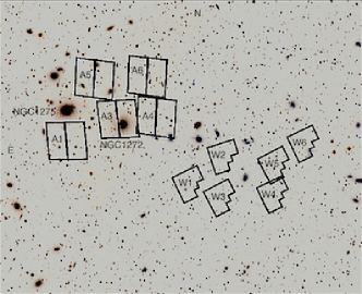
Figure 1: Image of the central region of the Perseus cluster (DSS image in blue IIIaJ), showing the locations of the HST images used in this study. North is at top, East at left. The field shown is $36^{\prime}$ across, corresponding to 750 kpc at the distance of Perseus. Note that field ACS-1 is below the central cD NGC 1275, while field ACS-3 contains NGC 1272.

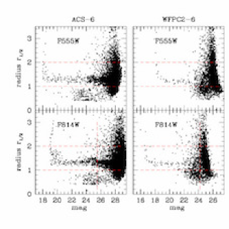
Figure 2: Left panels: SourceExtractor parameters $r_{1/2}$ versus aperture magnitude, for both filters in ACS field 6. Right panel: The same quantities for WFPC2 field 6. Units of $r_{1/2}$ are pixels, where 1 px = $0.05^{\prime\prime}$ for ACS and $0.1^{\prime\prime}$ for WFPC2. Objects in the ‘starlike’ range $1<r_{1/2}<2$ are selected for further photometry with daophot/allstar. Vertical dashed lines show the $F814W$ magnitude limit adopted for analysis of the GC populations (see text).

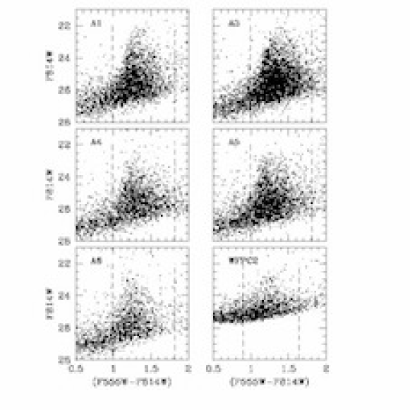
Figure 3: Color-magnitude diagrams for the measured unresolved (starlike) objects in the Perseus fields. The five ACS/WFC fields are labelled A1,3,4,5,6, while the six WFPC2 fields are combined into one CMD at lower right. The vertical dashed lines at $(F555W-F814W)=0.99,1.81$ (for ACS) and $0.89,1.64$ (for WFPC2) mark the (generous) range of colors populated by normal globular clusters. The detection limit ($m_{0}$ in Table 1) for the WFPC2 fields is clearly much brighter than for the ACS fields because of shorter exposure times and lower detector sensitivity.

At 75 Mpc distance, a typical GC half-light diameter $\simeq 4$ pc converts to an image FWHM of 0.01 arcsec, an order of magnitude smaller than the resolution limit of the HST cameras (see also Harris, 2009a, for discussion). The great majority of the GCs in the Perseus galaxies will therefore be comfortably starlike in appearance, which greatly simplifies the process of GC candidate object selection and photometry. Essentially, we look for unresolved objects within each ACS or WFPC2 field that also fall within the (fortunately) relatively narrow color range in $(V-I)$ that match real GCs. As will be seen below, the combination of image morphology and color eliminates almost all contaminants in the sample (foreground field stars, or very faint small background galaxies).

Data reduction began with the *.flc image files from the HST Archive. For each of the target fields, the individual exposures (4 in each filter) were registered and combined with stsdas/multidrizzle into a single composite exposure in each filter. Total exposure times for each ACS/WFC field are 2260 s ($F814W$) and 2368 s ($F555W$). For each of the 6 WFC2 fields, total integration times in each filter were 1900 s.

The procedure for detection and photometry of the GC candidates then followed the steps outlined in, e.g., Harris (2009a); Harris et al. (2016). SourceExtractor (SE) (Bertin & Arnouts, 1996) was used to detect objects and to do a preliminary rejection of nonstellar ones (either single-pixel artifacts or faint background galaxies) from a plot of the SE parameters $r_{1/2}$ versus aperture magnitude. Samples of these for one ACS field and one WFPC2 field are shown in Figure 2. Starlike (point-source) objects fall near $r_{1/2}\simeq 1.3$ px and objects with $r_{1/2}<1$ or $>2$ in either filter were rejected. Final photometry of the candidates was done through the tools in iraf/daophot, including point-spread-function (PSF) fitting and allstar solutions, then corrected to equivalent large-aperture magnitudes. The PSF in each field was determined empirically from moderately bright, uncrowded stars. The object lists in each filter were matched to within $0.1^{\prime\prime}$ and any objects not appearing in both filters were rejected. Finally, objects with poor goodness-of-fit to the PSF ($\chi>2$) or large photometric uncertainties ($\sigma>0.3$ mag) were also rejected. The combination of steps (SE parameters, $\chi$ and $\sigma$ rejection, matching lists in both filters) proved to be quite effective at culling nonstellar objects. We note that rejection of nonstellar objects is not expected to be as rigorous on the WFPC2 fields, which have a larger pixel size than ACS/WFC ($0.1^{\prime\prime}$ versus $0.05^{\prime\prime}$) and shorter exposure times as well. Within the WFPC2 array we used the WF2, WF3, and WF4 detectors but not the small PC1, to avoid issues with different limiting magnitudes and resolution.

Photometric completeness as a function of magnitude was evaluated through daophot/addstar tools, where scaled PSFs are added to the images and then the process of detection and photometry is repeated. Since every one of the target fields is quite uncrowded in absolute terms, artificial-object lists were generated randomly in location across the field. The dependence of completeness $f(m)$ (the fraction of successfully detected and measured objects versus magnitude) is modelled with the simple two-parameter function (Harris et al., 2016) $f=(1+\mathrm{exp}(\alpha(m-m_{0}))^{-1}$, where $m_{0}$ is the magnitude at which 50% of the objects are detected and $\alpha$ measures the steepness of falloff of the completeness curve. In Table 1 we list the $(\alpha,m_{0})$ pairs for each ACS field individually; as expected, they are closely similar from one field to the next. For the WFPC2 fields we list the average of the 6 fields.

In the following discussion, we present the color-magnitude data in the natural filter magnitudes $(F555W,F814W)$. For ACS/WFC these can be transformed to $(V,I)$ through (Saha et al., 2011)

$$(V-I)\,=\,0.912(F555W-F814W)\,$$ (1)

$$I\,=\,F814W+0.024(V-I)$$ (2)

while for WFPC2 the adopted transformation is (Holtzman et al., 1995)

$$(V-I)\,=\,1.010(F555W-F814W)\,$$ (3)

$$I\,=\,F814W-0.062(V-I)\,.$$ (4)

3 Analysis

3.1 Color-Magnitude Distributions

In Figure 3 the distribution of measured unresolved (starlike) objects in the color-magnitude diagram (CMD) is shown, for each of the five ACS fields and for all six WFPC2 fields combined. In the $(I,V-I)$ plane, normal GCs will fall well within a generous color range $(V-I)_{0}\simeq 0.70-1.45$ (Larsen et al., 2001) where color is primarily a function of cluster metallicity. Thus for our adopted reddening $E_{V-I}=0.202$, this range of intrinsic colors translates into $(F555W-F814W)\simeq 0.99-1.81$ (ACS) or $\simeq 0.89-1.64$ (WFPC2).

In every ACS field a substantial population appears in this target range, dominating all objects with $I\lesssim 26$. (Note that the swath of points along the bottom running diagonally up from lower left is at or below the completeness limit of the photometry and thus mostly represent extremely uncertain detections or noise). Adding to the evidence for their identification as GCs is that the bright end effectively stops near $I\simeq 22$, which translates to $M_{I}=-12.5$ or roughly $M_{V}=-11.5$ for a mean intrinsic color $(V-I)_{0}=1.0$. The luminosity distribution of normal GCs (GCLF) is highly consistent between galaxies, and reaches a “top end” at $M_{I}\simeq-12.5$ even for the most luminous galaxies with the biggest GC populations (Harris et al., 2014).

Looking further into the CMDs, in most galaxies the GC population falls into a bimodal distribution where “blue” (metal-poor) ones peak near $(V-I)_{0}\simeq 0.95$ and “red” (metal-richer) ones near $(V-I)_{0}\simeq 1.15$ (e.g. Larsen et al., 2001). For the Perseus fields these translate to mean colors $(F555W-F814W)=1.25$ and 1.50 (ACS filters). Both the blue and red sequences can be seen at these colors in the five ACS fields. The actual color distribution functions will be discussed in more detail below.

In the combined WFPC2 fields (lower right panel of Fig. 3), the scatter of the photometry is larger and the limiting magnitudes shallower. Nevertheless, a thinly populated sequence of objects with $F814W<24$ and near $(F555W-F814W)\simeq 1.2$ is clearly present. This mean color is equivalent to $(V-I)_{0}=1.0$, exactly the mean intrinsic color of normal GCs. The presence of this sequence is the first evidence that these outlying fields have a sparsely spread GC population.

3.2 Luminosity Distributions

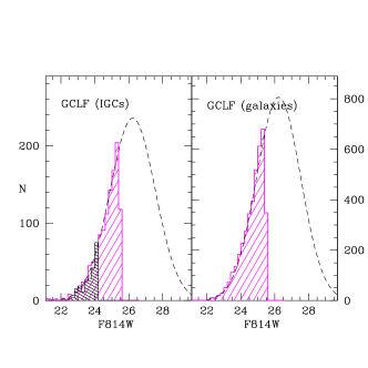
Figure 4: Number of objects per 0.2-mag bin in $F814W$, plotted versus magnitude. Left panel: The magenta histogram gives the numbers for the fields ACS-4 and ACS-6 combined, which should be dominated by IGCs. For $F814W<25.5$ the photometric completeness is near 100%. The black shaded histogram gives the numbers for the 6 outlying WFPC2 fields combined, over the range $F814W<24.2$ where photometric completeness is high. The Gaussian curve shown as the dashed line has a turnover (peak) at $F814W=26.2$ and standard deviation 1.33 mag. Right panel; The magenta histogram gives the numbers per 0.2-mag bin in the fields ACS-1,3,5 combined; these are dominated by the giant ellipticals in the Perseus core. The Gaussian dashed line has a standard deviation 1.30 mag and the same turnover as in the left panel.

A further test of ‘normal’ old GC populations is that they should follow a Gaussian-like distribution in number per unit magnitude (e.g. Jordán et al., 2007; Villegas et al., 2010; Harris et al., 2014). For the Perseus data, we anticipate that fields ACS-1,3,5 should be predominantly populated by GCs from the giant ellipticals in the Perseus core, while ACS-4,6 and the WFPC2 fields should have a much higher fraction of IGCs if they are present (see next section for the spatial distributions). In Figure 4, we show the luminosity functions for these three groups of fields separately.

A typical GCLF based on the data for individual galaxies of all luminosities (see the references cited above) should have a Gaussian turnover (peak) luminosity $M_{V}\simeq-7.3$, $M_{I}\simeq-8.3$ (assuming a mean $(V-I)\simeq 1.0$), and a standard deviation $\sigma\simeq 1.3$ mag. Both the turnover and width of the fiducial GCLF are empirically uncertain by $\sim 0.1$ mag (e.g. Jordán et al., 2007). For Perseus, the GCLF turnover would then be expected to lie at $I\simeq 26.2$, which is fainter than the useful photometric limits in the ACS fields and considerably fainter than the WFPC2 field limit.

Since the data fall short of the turnover magnitude $m_{0}$, both $m_{0}$ and $\sigma$ cannot be solved simultaneously very accurately (e.g. Hanes & Whittaker, 1987), so instead we simply assume $m_{0}(F814W)=26.2$ and solve for $\sigma$ as a consistency test of the Gaussian form. To do this, we used the objects in a restricted magnitude range $F814W<25.5$ (for the ACS fields) within which the photometric completeness is nearly 100% and the CMD is minimally affected by either field contamination or spread of photometric errors. The histograms of number per 0.2-mag bin in that range are shown in Fig. 4. Least-squares fits of a Gaussian curve yield $\sigma=1.30\pm 0.03$ mag for ACS-1+3+5 (the fields dominated by Perseus core galaxies), and $\sigma=1.33\pm 0.04$ mag for ACS-4+6. In both cases the model curve fits the data closely. In the left panel of Fig. 4 the LF for the combined WFPC2 fields is also shown, indicating that these outer regions are also consistent with the assumption of a normal GCLF.

3.3 Background

Assessing whether or not we are looking at an IGC population, particularly for the sparse outer WFPC2 fields, also requires having some idea of the level of field contamination. The best way to do this would be through control fields from WFC3, ACS/WFC, or WFPC2 located close to but outside Perseus and with the same filters and similar exposure times. Unfortunately a search of the HST Archive did not yield any useful cases.

Figure 5: Solid dots: Color-magnitude diagrams for a simulated Milky Way population of stars in the direction of NGC 1275, generated by TRILEGAL. This example is for an area on the sky equal to 5 ACS/WFC fields combined. The dashed lines enclose the expected range of magnitude and colors for GCs in the Perseus galaxies. Circled crosses: Starlike objects in the HUDF (see text).

One alternative is to estimate the expected number of foreground stars with a Milky Way stellar population model. In Figure 5, we show a sample CMD produced by TRILEGAL (Girardi et al., 2005) in the direction of NGC 1275 and comprising an area equal to all 5 ACS fields combined. Since the projected area on the sky is small, different random realizations of TRILEGAL show large stochastic differences, but the example shown here is typical. Only $\sim 10$ stars appear within the broad magnitude and color range for the Perseus GCs, and most of these are too bright and red to fall within the normal GC sequences described above.

Contamination may also arise from faint, very compact background galaxies that slip through the initial rejection criteria (SE parameters, $\chi$, magnitude uncertainty, and color range). To estimate the numbers of such objects that we would expect per ACS field, data from the Hubble Ultra-Deep Field (HUDF) were used as provided from the catalogs at heasarc.gsfc.nasa.gov/W3Browse/hst/hubbleudf.html. Fig. 5 shows the HUDF objects that can be classified as starlike ($r_{1/2}<2$ px from SourceExtractor) and fall in the color range of interest. (Note that these objects were made fainter and redder by $A_{V}=0.447,E_{V-I}=0.202$ to match the Perseus field.) The vast majority of ‘starlike’ objects in the HUDF are much fainter than our target range, and most of the rest are too blue or red to match GC colors. The remainder consist of only a handful of contaminants with $I\gtrsim 24.5$ and within the color range marked in Fig. 5. Much the same result was found in a very similar study of the GC population around NGC 6166 (Harris et al., 2016) (see especially Figs. 8 and 9 there).

For each of the ACS fields, the field contamination should then make up less than 1% of the observed numbers of objects in our CMDs (Fig. 3), so we do not remove any background from the LFs or the radial distributions described below. For the WFPC2 fields, as seen for the discussions of the luminosity function and color distribution function, we use only the objects with $I<24.0$, which further excludes the contaminating objects in Fig. 5 almost totally.

In summary, the current material points to the presence of a significant population of bona fide GCs around the Perseus galaxies. These objects follow the distributions expected for normal GCs in terms of their magnitude, color, and unresolved size. We can now continue to a discussion of their spatial distribution within Perseus and relative to the two dominant galaxies, NGC 1272 and 1275.

3.4 Spatial Distributions

As seen in Fig. 3, the largest GC populations are in fields ACS-1 (which is nearest NGC 1275) and ACS-3 (which includes NGC 1272). The star-cluster population in NGC 1275 itself has been discussed briefly by Carlson et al. (1998), Canning et al. (2010), and Penny et al. (2012), derived from WFPC2 and ACS images centered on the galaxy (though in different filters) that we do not use here. In total, the NGC 1275 star clusters consist of a mixture of old GCs spread throughout the galaxy’s halo, plus a rich population of younger clusters located along its spectacular network of H$\alpha$ filaments.

Since NGC 1275 is the central giant, we first plot the GC number density versus radial distance from it. The results are shown in Figure 6. Here, the number of GCs per unit projected area on the sky $\sigma_{cl}$ is calculated within radial annuli centered on NGC 1275. For the ACS fields, the GCs used in the sums include objects with $F814W<25.5$, $1.0<(F555W-F814W)<1.8$. At the adopted limit $F814W(lim)=25.5$, the internal photometric errors in the ACS data are $e_{I}=\pm 0.10$, $e_{V-I}=\pm 0.13$.

Placing the raw WFPC2 counts on the same graph as the ACS fields requires scaling them to the same magnitude limit. To do this, we truncate the adopted limiting magnitude now more severely to $F814W<23.5$, $0.9<(F555W-F814W)<1.65$ to avoid the fainter cloud of points which may be dominated by small faint background galaxies and even artefacts that escaped the photometric culling. At $F814W=23.5$ the internal photometric errors are $e_{I}=\pm 0.06$, $e_{V-I}=\pm 0.11$. A useful test of contamination is the field-to-field scatter in the numbers of detected objects. For $F814W(lim)=24.2$, we find that the scatter amongst the 6 WFPC2 fields is much larger than the $\sqrt{N}$ level expected from simple count statistics, which would be the expected result from the known physical clustering of faint background galaxies over several arcminutes scale. By comparison, for $F814W(lim)\lesssim 23.5$, the field-to-field scatter is near $\sqrt{N}$, indicating that most of the contaminating galaxies are gone. From the ACS counts, there are 1210 objects with $F814W\leq 25.5$ and within the desired color range, but only 131 with $F814W\leq 23.5$. The WFPC2 counts are therefore scaled up by the ratio ($9.24\pm 0.85$) to give the equivalent number brighter than $F814W=25.5$. These renormalized $\sigma-$values for the individual WFPC2 fields are plotted in Fig. 6 along with the value from all 6 fields combined.

In Fig. 6 the different regions are color-coded for easier distinction:

ACS-1 shows the outer NGC 1275 halo, and the strong radial falloff of $\sigma_{cl}$ relative to its center is evident. The power-law slope shown in the Figure is well defined by the data and has slope $\alpha=(\Delta{\rm log}\sigma_{cl}/\Delta{\rm log}R)=-1.67\pm 0.01$. This deduced slope agrees well with $\alpha=-1.6$ found by Penny et al. (2012) based on both ACS-1 and ACS/WFC images centered on the galaxy.

ACS-3 encloses the giant NGC 1272 and its GC population is clearly dominated by it (see Canning et al., 2010; Penny et al., 2012), so it is not plotted in Fig. 6 relative to the center of NGC 1275. It will be discussed in Section 4 below.

ACS-4 may be a combination of NGC 1272 halo and IGC; for it, we find a radial falloff $\alpha=-2.20\pm 0.50$.

ACS-5, from its location and $\sigma_{cl}$ behavior, suggests that we are looking at a combination of populations from the outer halos of both NGC 1275 and NGC 1272, plus some less certain contributions from the smaller ellipticals in the field and the IGCs. The formal solution for the radial falloff gives $\alpha=-0.87\pm 0.19$.

ACS-6 is farthest from both the major galaxies, so the IGC component should be relatively more dominant. A shallow and uncertain radial falloff is seen with $\alpha=-0.9\pm 0.4$.

WFPC2: the WFPC2 fields contain no major Perseus galaxies and are located radially from $R=270$ to 530 kpc from the Perseus center, and should therefore give us a fairly clean IGC sample (though unfortunately to shallower magnitude limits, as discussed above). Interestingly, the 6 points in Fig. 6 show an internally uncertain but distinctive downward radial gradient, with the exception of the outermost W6. The number density for all 6 of these fields combined is $\langle\sigma_{cl}\rangle=(0.0042\pm 0.0007)$ arcsec^-2, shown by the large open symbol and errorbar. The solid line drawn through the points has a slope $\alpha\simeq-1.2$ and seems at least roughly to continue the outward trend from ACS-6. Though the field coverage is admittedly only a small fraction of the Perseus core and outskirts, these data hint that we may be observing the radial distribution of the IGC component, far from any major member galaxies.

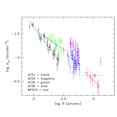
Figure 6: Number of objects per arcsec², plotted versus radial distance from NGC 1275 (the Perseus center). To be used in this diagram, a measured object needed to be (a) starlike, (b) in the color range shown in Fig. 3, and (c) brighter than $F814W=25.5$ (see text). The data are color-coded by field location. For each ACS field the best-fitting power law curve $\sigma_{cl}\sim R^{\alpha}$ is drawn in. For the WFPC2 fields (in red symbols), the mean point (large open symbol) is the total number in all 6 fields divided by their total area.

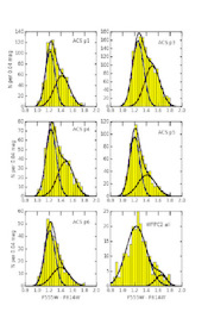
Figure 7: GMM fits to the color distribution functions in the five ACS fields and (at lower right) the combined data from the WFPC2 fields. The histograms in yellow shows the number of objects in bins of width 0.04 mag in color. In each panel, the solid lines show the best-fit blue and red modes, and the sum of the two modes as the upper envelope.

3.5 Metallicity and Color Distributions

Table 2: Bimodal Gaussian Fits to the CDF

Field	$\mu_{1}$	$\mu_{2}$	$\sigma_{1}$	$\sigma_{2}$	$f(red)$	$D$
ACS-1	1.221(0.008)	1.419(0.019)	0.081(0.004)	0.130(0.008)	0.472(0.057)	1.82(0.21)
ACS-3	1.262(0.016)	1.503(0.029)	0.095(0.007)	0.129(0.011)	0.456(0.086)	2.12(0.20)
ACS-4	1.237(0.014)	1.481(0.033)	0.089(0.007)	0.136(0.013)	0.443(0.087)	2.13(0.29)
ACS-5	1.204(0.010)	1.409(0.023)	0.087(0.005)	0.149(0.006)	0.381(0.058)	1.69(0.15)
ACS-6	1.215(0.016)	1.397(0.046)	0.089(0.010)	0.145(0.015)	0.357(0.110)	1.51(0.40)
WPC2	1.233(0.022)	1.649(0.075)	0.174(0.014)	0.094(0.025)	0.091(0.069)	2.97(0.53)

The distribution of GC colors (CDF) is driven to first order by the underlying metallicity distribution function (MDF). As noted above, in most galaxies the CDF and MDF are bimodal, with a canonical metal-poor (MP) “blue” sequence centered near $\langle$[Fe/H]$\rangle\simeq-1.5$ and a metal-rich (MR) “red” sequence near $\langle$[Fe/H]$\rangle\simeq-0.5$ (e.g. Zepf & Ashman, 1993; Forbes et al., 1997, 2011; Brodie & Strader, 2006; Arnold et al., 2011; Blom et al., 2012; Cantiello et al., 2014; Brodie et al., 2014; Kartha et al., 2016, among many others). A numerically convenient way to characterize the two modes is by their Gaussian mean colors ($\mu_{1},\mu_{2}$) (blue, red) and dispersions ($\sigma_{1},\sigma_{2}$), as well as the fraction of total number of GCs in each mode, ($f_{1},f_{2}$) where $f_{1}+f_{2}\equiv 1$.

For each field in this study, a bimodal-Gaussian fit to the CDF was done with the GMM code (Muratov & Gnedin, 2010). The color histograms are displayed in Figure 7, and in Table 2 the details for the GMM fits are summarized. The last column gives the statistic $D=(\mu_{2}-\mu_{1})/\sqrt{(\sigma_{1}^{2}+\sigma_{2}^{2}/2}$, which is an estimate of the degree of separation of the two modes (bimodality favored if $D\gtrsim 2$). The data included for these fits are the same datasets restricted by magnitude and color as defined in Section 3.4 above.

The five ACS fields give highly consistent results for the mean colors $\mu_{1},\mu_{2}$ and dispersions $\sigma_{1},\sigma_{2}$ of the blue and red modes. The $D$ statistic is near $D\sim 2$ and the raw histograms are asymmetric for all the fields, suggesting that intrinsic bimodality is preferred over unimodality. In addition, the $p-$statistic giving the probability for unimodality (the null hypothesis) is $p\ll 0.01$ for all 5 ACS fields, strongly favoring bimodality. The red (metal-richer) fraction $f_{2}=f_{red}$ decreases gradually outward from the Perseus center, as expected by comparison with Virgo and Coma (Durrell et al., 2014; Peng et al., 2011). That is, metal-richer (redder) GCs are more centrally concentrated within galaxies and are in any case not as numerous as the blue (metal-poor) ones in the smaller galaxies that should have been the main progenitors for the ICL.

Converting the $(F555W-F814W)$ values in Table 2 to intrinsic color $(V-I)_{0}$ for the 5 ACS fields gives mean dereddened values $(V-I)_{0}=0.92$ (blue mode) and 1.11 (red mode). These are both within the ranges of $(\mu_{1},\mu_{2}$) for normal early-type galaxies; for example, Larsen et al. (2001) find mean colors $(V-I)_{0}=0.90-0.99$ for the blue mode and $1.10-1.21$ for the red mode, systematically increasing with host galaxy luminosity. Again, if the ICL is dominated by material stripped from $L_{\star}-$type galaxies (see above), then we would expect the mean colors $\mu_{1},\mu_{2}$ both to be a bit bluer than for the giant galaxies.

The results for the WFPC2 field are considerably more uncertain because of the shallower magnitude limit and smaller sample size. The blue component lies at $\mu_{1}=1.23$, corresponding to $(V-I)_{0}=1.04$, which is between the standard blue and red modes described above. The nominal red component $\mu_{2}$ is small (only 9% of the total) and we cannot rule out that it is due simply to some residual field contamination (see above) combined with greater photometric error than in the ACS fields.

For the combined WFPC2 fields, the GMM solution gives $p=0.055$, which does not strongly favor intrinsic bimodality. In addition, the blue-mode dispersion $\sigma_{1}=0.17$ is twice as large as the blue-mode dispersions in the deeper ACS fields. The main population $f_{1}$ may therefore simply be a combination of the normal blue and red modes blurred together by the higher photometric uncertainty. If we restrict the sample further to $F814W<23.5$ as in Section 3.4 above, a GMM fit yields similar results: the nominal blue and red modes are not separated and the color distribution is not clearly different from unimodal. Deeper and more precise photometry will be required to reach a clearer answer.

4 NGC 1272 and 1275

The placement of the ACS fields allows a good opportunity to determine the spatial distribution of the NGC 1272 GC system in particular. ACS-3 contains the galaxy, while ACS-4 and ACS-6 are immediately adjacent and (helpfully) sit on the opposite side from NGC 1275. (ACS-5 is equidistant from both NGC 1272 and 1275 and its GC population might be expected to comprise a roughly equal mixture of the two; see again Fig. 6.) In Figure 8 (upper panel), the number density $\sigma_{cl}$ (objects per arcsec^-2) is plotted for ACS-3,4,6 relative to the center of NGC 1272. Here $\sigma_{cl}$ decreases smoothly outward, converging to a near-constant level at the largest radii sampled. From the outermost 6 bins (containing 124 objects) in ACS-6 we adopt a background $\sigma_{b}=0.0075\pm 0.00067$ arcsec^-2, indicated by the dashed line in Fig. 8. As noted above, this $\sigma_{b}$ is only slightly larger than the level of the inner the WFPC2 fields (Fig. 6), suggesting again that ACS-6 is sampling primarily the IGC population. Subtracting this $\sigma_{b}$ from the radial profile gives the result shown in Figure 9. A Sérsic-type function (Sérsic, 1968) given by

$$\sigma_{cl}\,=\,\sigma_{e}{\rm exp}(-b_{n}[({R\over R_{e}})^{1/n}-1])$$ (5)

matches the result accurately, with best-fit parameters $n=1.3$, $R_{e}=153^{\prime\prime}$, $\sigma_{e}=0.0122$ arcsec^-2, $b_{n}=2.46$.

Integration of the model profile out to $R\simeq 500^{\prime\prime}$ yields a total of $N=3570\pm 150$ GCs brighter than our adopted limit $F814W=25.5$. This limit is 0.7 mag brighter than the expected GCLF turnover point $F814W(to)=26.2$ (Fig. 4). Extrapolating in turn to find the total number of GCs over all magnitudes then yields $N_{GC}=12000\pm 1400$, where the stated uncertainty includes the Poisson count statistics, a $\pm 0.1-$mag uncertainty in the GCLF turnover luminosity, and a $\pm 0.1-$mag uncertainty in the GCLF dispersion. Finally, the GCS specific frequency (Harris & van den Bergh, 1981) is $S_{N}=N_{GC}\cdot 10^{0.4(M_{V}^{T}+15)}=7.9\pm 0.9$, a moderately high value within the typical range for supergiant ellipticals (cf. Harris et al., 2013). A remaining question is whether or not the GCS from NGC 1275 itself is contributing to the NGC 1272 totals particularly in ACS-3. From the NGC 1275 profile (see comments below and the lower panel of Fig. 8), it appears that the contribution from NGC 1275 at the $300^{\prime\prime}=$ 110 kpc projected distance of NGC 1272 will be at the level of only a few percent. If and when more complete imaging coverage of the core Perseus region is available, it will be possible to solve for the spatial distributions of both galaxies simultaneously and more accurately (see e.g. Wehner et al., 2008, for an example in the Hydra cluster).

For the central giant NGC1275, the available material is much more limited and the conclusions about total GC population correspondingly rougher. We use field ACS-1 along with ACS-6 to set the local background, though here we are forced to assume that $\sigma_{b}$ is roughly constant over the region concerned. The measurements are shown in the lower panel of Fig. 8, replotted from Fig. 6. The combination of this radial profile and the inner data from Penny et al. (2012) indicates that $\sigma_{cl}\sim R^{-1.6}$ from $R\simeq 60^{\prime\prime}$ outward, and is relatively flat inside $60^{\prime\prime}$. The main concerns in estimating its total population are the true local background level, and how far outward the NGC 1275 halo extends before fading into the ICM; the present data do not answer either of these satisfactorily. Here we simply use an outer radius $R_{max}=270^{\prime\prime}$ (100 kpc) for integration of the profile and $\sigma_{b}\simeq 0.0075\pm 0.00067$ arcsec^-2 as above. The result is then $N=3990\pm 380$ GCs for $F814W<25.5$, not including any (unknown) systematic error in the adopted background. Extrapolating over all magnitudes as described above gives $N_{GC}=13500\pm 2000$ and a specific frequency $S_{N}=12.2\pm 1.8$, including $\pm 0.1-$mag uncertainties in the GCLF turnover and dispersion as above. This total GC population and $S_{N}$ would make NGC 1275 quite similar to M87 in Virgo (e.g. Harris, 2009b).

We emphasize once again that a better assessment will require a wider-field survey in which the GC populations in the member galaxies, and the IGCs, can both be determined more completely. Nevertheless, this very limited imaging material is enough to suggest that both of the dominant Perseus galaxies appear to have very populous GC systems. The closest analogy may be the more well known Coma cluster, where both NGC 4874 and 4889 have similarly large GC populations but where the central cD (NGC 4874) has the higher specific frequency.

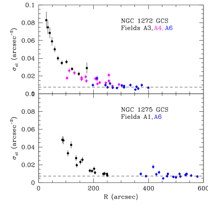
Figure 8: Upper panel: Radial distribution of unresolved (starlike) objects centered on NGC 1272, within the magnitude range $21<F814W<25.5$ and color range $1.0<(F555W-F814W)<1.8$ (see text). Data from fields ACS-3 (black symbols), ACS-4 (magenta), and ACS-6 (blue) are shown here. The projected density per unit area $\sigma_{cl}$ is plotted versus projected radius $R$ from the center of NGC 1272. The dashed line at $\sigma=0.0075$ is the adopted background level. Lower panel: Radial distribution for unresolved objects in fields ACS-1 (black) and ACS-6 (blue), where $R$ is now the radius from the center of NGC 1275.

Figure 9: Radial distribution of the GC system around NGC 1272, after background subtraction. The datapoints include the numbers from ACS-3 and 4. The best-fit Sérsic function as described in the text is shown as the solid line.

5 Discussion: The IGC Population

The data discussed in this paper consist of only 11 pencil-beam probes of the GC population, and thus fall far short of a genuine wide-field survey of the Perseus cluster. Only a more comprehensive survey to similar depth will be able to address the true spatial distribution of the IGCs and their total number.

Nevertheless, we can make a very rough attempt to gauge the total GC population. We assume, following Figs. 6 and 8, that $\sigma(IGC)$ is approximately constant at $\sigma_{0}\simeq 0.0078$ arcsec^-2 in the inner part of the cluster and then falls off as $\sim R^{-1.2}$ further out. The inflection point where the power law reaches $\sigma_{0}$ is at $R=500^{\prime\prime}$ = 180 kpc from cluster center. Integrating $\sigma(IGC)$ out to the most remote field, WFPC2-6 at $R=0.38^{o}$ = 500 kpc, then gives $N\simeq 24,000$ GCs brighter than $F814W=25.5$. Extrapolating over the entire GCLF yields $N_{IGC}\sim 82000$ IGCs over this radial range. To emphasize its limitations once again, it is obvious that this argument works forward from an extremely limited sampling of the Perseus region, so it cannot account for any details and asymmetries of the IGM spatial structure.

In Coma Peng et al. (2011) trace the IGC component out to $R\sim 500$ kpc and find that it must fall rapidly outside of that. Durrell et al. (2014) measure the Virgo IGCs out to $R\simeq 700$ kpc from the center of M87, again finding that their number density falls rapidly after that. The Perseus results, though quite tentative, fall into the same general pattern.

A better way to estimate the total GC population in Perseus at this stage may be to use the mass ratio $\eta_{M}\equiv(M_{GCS}/{M_{h}})$ where $M_{GCS}$ is the total mass in all the GCs and $M_{h}$ is the total mass in the entire cluster, dark plus baryonic (roughly, its virial mass $M_{200}$). Empirically, $\eta_{M}$ has been found to be nearly constant over a wide range of environments including dwarf or giant galaxies, spirals or ellipticals, and entire galaxy clusters; see, e.g., Blakeslee et al. (1997); Spitler & Forbes (2009); Durrell et al. (2014); Hudson et al. (2014); Harris et al. (2015, 2017). The most recent calibration gives $\langle\eta_{M}\rangle=(4.3\pm 0.6)\times 10^{-5}$ for entire clusters of galaxies (Harris et al., 2017). For the Perseus cluster, $M_{200}=(6.65\pm 0.45)\times 10^{14}M_{\odot}$ from Simionescu et al. (2011) determined from its X-ray gas pressure profile. If we then take a mean GC mass $M_{GC}=2.8\times 10^{5}M_{\odot}$ appropriate for $L_{\star}$ galaxies (Harris et al., 2017), the resulting estimate of the total population is $N_{GC}=102,000$ clusters. If analogies with Virgo or Coma are useful, roughly half of these should belong to the member galaxies, with the remainder in the IGM; thus, $N_{IGC}\sim 50,000$, which agrees to within a factor of two with our estimate working directly from the observations. GC populations this large are not unprecedented: Coma, which has a total mass very similar to Perseus, contains at least $N_{GC}=70,000$ GCs (Peng et al., 2011), and estimates well above $N_{GC}=100,000$ have been proposed for the more distant clusters A1689 and A2744 (Alamo-Martínez et al., 2013; Lee & Jang, 2016).

This range of estimates for $N_{GC}$, though admittedly crude, indicates that the Perseus IGC component may be quite comparable with the Virgo and Coma clusters, and reinforces the growing evidence that rich clusters of galaxies contain large amounts of intragalactic stellar light. Though far more dilute, the ICL may add up to as much stellar mass as is in the galaxies, and is the visible tracer of a long history of galaxy interaction and tidal stripping.

6 Summary

We have used photometry from HST ACS and WFPC2 imaging within the rich Perseus cluster (Abell 426) to isolate its globular cluster population and to attempt detection of an Intragalactic population. Our principal findings are these:

1. In the target fields, GC populations are clearly present following a normal Gaussian distribution versus magnitude and a bimodal distribution in $(V-I)$ color that matches the expected properties seen in individual galaxies.

2. In the core region of Perseus, large numbers of GCs are present, but these are dominated by the halos of the two largest galaxies in the region, NGC 1275 and NGC 1272. We estimate that NGC 1272 contains $\simeq 12000$ GCs with $S_{N}=7.9\pm 0.9$, while for the central giant NGC 1275 we estimate more crudely $N_{GC}\sim 13500$ and $S_{N}\sim 12$, very similar to M87.

3. The radial distribution of GCs counts indicates that an IGC component is present extending several hundred kpc away from the Perseus center. Two different methods lead to the (very tentative) conclusion that there may be $\sim 50000-80000$ IGCs in Perseus as a whole, which would make it comparable with the Virgo and Coma clusters.

4. A more comprehensive, wider-field survey of the Perseus cluster promises to be rewarded with a much more complete understanding of the Intragalactic cluster population and the entire ICL component.

References

- Adami et al. (2013) Adami, C., Durret, F., Guennou, L., & Da Rocha, C. 2013, A&A, 551, A20
- Alamo-Martínez et al. (2013) Alamo-Martínez, K. A., Blakeslee, J. P., Jee, M. J., et al. 2013, ApJ, 775, 20
- Arnaboldi et al. (2007) Arnaboldi, M., Gerhard, O., Okamura, S., et al. 2007, PASJ, 59, 419
- Arnold et al. (2011) Arnold, J. A., Romanowsky, A. J., Brodie, J. P., et al. 2011, ApJ, 736, L26
- Barbosa et al. (2016) Barbosa, C. E., Arnaboldi, M., Coccato, L., et al. 2016, A&A, 589, A139
- Bassino et al. (2003) Bassino, L. P., Cellone, S. A., Forte, J. C., & Dirsch, B. 2003, A&A, 399, 489
- Bender et al. (2015) Bender, R., Kormendy, J., Cornell, M. E., & Fisher, D. B. 2015, ApJ, 807, 56
- Bergond et al. (2007) Bergond, G., Athanassoula, E., Leon, S., et al. 2007, A&A, 464, L21
- Bertin & Arnouts (1996) Bertin, E., & Arnouts, S. 1996, A&AS, 117, 393
- Blakeslee et al. (1997) Blakeslee, J. P., Tonry, J. L., & Metzger, M. R. 1997, AJ, 114, 482
- Blom et al. (2012) Blom, C., Spitler, L. R., & Forbes, D. A. 2012, MNRAS, 420, 37
- Brodie & Strader (2006) Brodie, J. P., & Strader, J. 2006, ARA&A, 44, 193
- Brodie et al. (2014) Brodie, J. P., Romanowsky, A. J., Strader, J., et al. 2014, ApJ, 796, 52
- Burke et al. (2012) Burke, C., Collins, C. A., Stott, J. P., & Hilton, M. 2012, MNRAS, 425, 2058
- Burke et al. (2015) Burke, C., Hilton, M., & Collins, C. 2015, MNRAS, 449, 2353
- Canning et al. (2010) Canning, R. E. A., Fabian, A. C., Johnstone, R. M., et al. 2010, MNRAS, 405, 115
- Cantiello et al. (2014) Cantiello, M., Blakeslee, J. P., Raimondo, G., et al. 2014, A&A, 564, L3
- Carlson et al. (1998) Carlson, M. N., Holtzman, J. A., Watson, A. M., et al. 1998, AJ, 115, 1778
- Castro-Rodriguéz et al. (2009) Castro-Rodriguéz, N., Arnaboldi, M., Aguerri, J. A. L., et al. 2009, A&A, 507, 621
- Coccato et al. (2011) Coccato, L., Gerhard, O., Arnaboldi, M., & Ventimiglia, G. 2011, A&A, 533, A138
- Contini et al. (2014) Contini, E., De Lucia, G., Villalobos, Á., & Borgani, S. 2014, MNRAS, 437, 3787
- Cooper et al. (2015) Cooper, A. P., Gao, L., Guo, Q., et al. 2015, MNRAS, 451, 2703
- Da Rocha & Mendes de Oliveira (2005) Da Rocha, C., & Mendes de Oliveira, C. 2005, MNRAS, 364, 1069
- D’Abrusco et al. (2016) D’Abrusco, R., Cantiello, M., Paolillo, M., et al. 2016, ApJ, 819, L31
- DeMaio et al. (2015) DeMaio, T., Gonzalez, A. H., Zabludoff, A., Zaritsky, D., & Bradač, M. 2015, MNRAS, 448, 1162
- Durrell et al. (2014) Durrell, P. R., Côté, P., Peng, E. W., et al. 2014, ApJ, 794, 103
- Edwards et al. (2016) Edwards, L. O. V., Alpert, H. S., Trierweiler, I. L., Abraham, T., & Beizer, V. G. 2016, MNRAS, 461, 230
- Feldmeier et al. (2003) Feldmeier, J. J., Ciardullo, R., Jacoby, G. H., & Durrell, P. R. 2003, ApJS, 145, 65
- Ferguson et al. (1998) Ferguson, H. C., Tanvir, N. R., & von Hippel, T. 1998, Nature, 391, 461
- Forbes et al. (1997) Forbes, D. A., Brodie, J. P., & Grillmair, C. J. 1997, AJ, 113, 1652
- Forbes et al. (2011) Forbes, D. A., Spitler, L. R., Strader, J., et al. 2011, MNRAS, 413, 2943
- Gal-Yam et al. (2003) Gal-Yam, A., Maoz, D., Guhathakurta, P., & Filippenko, A. V. 2003, AJ, 125, 1087
- Giallongo et al. (2014) Giallongo, E., Menci, N., Grazian, A., et al. 2014, ApJ, 781, 24
- Girardi et al. (2005) Girardi, L., Groenewegen, M. A. T., Hatziminaoglou, E., & da Costa, L. 2005, A&A, 436, 895
- Gonzalez et al. (2005) Gonzalez, A. H., Zabludoff, A. I., & Zaritsky, D. 2005, ApJ, 618, 195
- Graham et al. (2015) Graham, M. L., Sand, D. J., Zaritsky, D., & Pritchet, C. J. 2015, ApJ, 807, 83
- Hanes & Whittaker (1987) Hanes, D. A., & Whittaker, D. G. 1987, AJ, 94, 906
- Harris (2009a) Harris, W. E. 2009a, ApJ, 699, 254
- Harris (2009b) —. 2009b, ApJ, 703, 939
- Harris et al. (2017) Harris, W. E., Blakeslee, J. P., & Harris, G. L. H. 2017, ApJ, 836, 67
- Harris et al. (2016) Harris, W. E., Blakeslee, J. P., Whitmore, B. C., et al. 2016, ApJ, 817, 58
- Harris et al. (2015) Harris, W. E., Harris, G. L., & Hudson, M. J. 2015, ApJ, 806, 36
- Harris et al. (2013) Harris, W. E., Harris, G. L. H., & Alessi, M. 2013, ApJ, 772, 82
- Harris & van den Bergh (1981) Harris, W. E., & van den Bergh, S. 1981, AJ, 86, 1627
- Harris et al. (2014) Harris, W. E., Morningstar, W., Gnedin, O. Y., et al. 2014, ApJ, 797, 128
- Holtzman et al. (1995) Holtzman, J. A., Burrows, C. J., Casertano, S., et al. 1995, PASP, 107, 1065
- Hudson et al. (2014) Hudson, M. J., Harris, G. L., & Harris, W. E. 2014, ApJ, 787, L5
- Iodice et al. (2016) Iodice, E., Capaccioli, M., Grado, A., et al. 2016, ApJ, 820, 42
- Jiménez-Teja & Dupke (2016) Jiménez-Teja, Y., & Dupke, R. 2016, ApJ, 820, 49
- Jordán et al. (2007) Jordán, A., McLaughlin, D. E., Côté, P., et al. 2007, ApJS, 171, 101
- Kartha et al. (2016) Kartha, S. S., Forbes, D. A., Alabi, A. B., et al. 2016, MNRAS, 458, 105
- Larsen et al. (2001) Larsen, S. S., Brodie, J. P., Huchra, J. P., Forbes, D. A., & Grillmair, C. J. 2001, AJ, 121, 2974
- Lee & Jang (2016) Lee, M. G., & Jang, I. S. 2016, ApJ, 831, 108
- Lee et al. (2010) Lee, M. G., Park, H. S., & Hwang, H. S. 2010, Science, 328, 334
- Longobardi et al. (2013) Longobardi, A., Arnaboldi, M., Gerhard, O., et al. 2013, A&A, 558, A42
- Martel et al. (2012) Martel, H., Barai, P., & Brito, W. 2012, ApJ, 757, 48
- McGee & Balogh (2010) McGee, S. L., & Balogh, M. L. 2010, MNRAS, 403, L79
- Melnick et al. (2012) Melnick, J., Giraud, E., Toledo, I., Selman, F., & Quintana, H. 2012, MNRAS, 427, 850
- Muratov & Gnedin (2010) Muratov, A. L., & Gnedin, O. Y. 2010, ApJ, 718, 1266
- Neill et al. (2005) Neill, J. D., Shara, M. M., & Oegerle, W. R. 2005, ApJ, 618, 692
- Peng et al. (2011) Peng, E. W., Ferguson, H. C., Goudfrooij, P., et al. 2011, ApJ, 730, 23
- Penny et al. (2011) Penny, S. J., Conselice, C. J., de Rijcke, S., et al. 2011, MNRAS, 410, 1076
- Penny et al. (2012) Penny, S. J., Forbes, D. A., & Conselice, C. J. 2012, MNRAS, 422, 885
- Presotto et al. (2014) Presotto, V., Girardi, M., Nonino, M., et al. 2014, A&A, 565, A126
- Purcell et al. (2007) Purcell, C. W., Bullock, J. S., & Zentner, A. R. 2007, ApJ, 666, 20
- Rudick et al. (2011) Rudick, C. S., Mihos, J. C., & McBride, C. K. 2011, ApJ, 732, 48
- Saha et al. (2011) Saha, A., Shaw, R. A., Claver, J. A., & Dolphin, A. E. 2011, PASP, 123, 481
- Sand et al. (2011) Sand, D. J., Graham, M. L., Bildfell, C., et al. 2011, ApJ, 729, 142
- Schuberth et al. (2008) Schuberth, Y., Richtler, T., Bassino, L., & Hilker, M. 2008, A&A, 477, L9
- Seigar et al. (2007) Seigar, M. S., Graham, A. W., & Jerjen, H. 2007, MNRAS, 378, 1575
- Sérsic (1968) Sérsic, J. L. 1968, Atlas de galaxias australes
- Simionescu et al. (2011) Simionescu, A., Allen, S. W., Mantz, A., et al. 2011, Science, 331, 1576
- Spitler & Forbes (2009) Spitler, L. R., & Forbes, D. A. 2009, MNRAS, 392, L1
- Urban et al. (2014) Urban, O., Simionescu, A., Werner, N., et al. 2014, MNRAS, 437, 3939
- Ventimiglia et al. (2011) Ventimiglia, G., Arnaboldi, M., & Gerhard, O. 2011, A&A, 528, A24
- Villegas et al. (2010) Villegas, D., Jordán, A., Peng, E. W., et al. 2010, ApJ, 717, 603
- Wehner et al. (2008) Wehner, E. M. H., Harris, W. E., Whitmore, B. C., Rothberg, B., & Woodley, K. A. 2008, ApJ, 681, 1233
- West et al. (2011) West, M. J., Jordán, A., Blakeslee, J. P., et al. 2011, A&A, 528, A115
- Williams et al. (2007) Williams, B. F., Ciardullo, R., Durrell, P. R., et al. 2007, ApJ, 654, 835
- Zepf & Ashman (1993) Zepf, S. E., & Ashman, K. M. 1993, MNRAS, 264, 611