New numerical methods for blow-up problems

Abstract

Two new methods of numerical integration of Cauchy problems for ODEs with blow-up solutions are described. The first method is based on applying a differential transformation, where the first derivative (given in the original equation) is chosen as a new independent variable. The second method is based on introducing a new non-local variable that reduces ODE to a system of coupled ODEs. Both methods lead to problems whose solutions do not have blowing-up singular points; therefore the standard numerical methods can be applied. The efficiency of the proposed methods is illustrated with several test problems.

1 Introduction

We will consider Cauchy problems for ODEs, whose solutions tend to infinity at some finite value of $x$, say $x=x_{*}$. The point $x_{*}$ is not known in advance. Similar solutions exist on a bounded interval and are called blow-up solutions. This raises the important question for practice: how to determine the position of a singular point $x_{*}$ and the solution in its neighborhood by numerical methods. In general, the blow-up solutions, that have a power singularity, can be represented in a neighborhood of the singular point $x_{*}$ as

$$y\approx A|x_{*}-x|^{-\beta},\quad\ \beta>0,$$

where $A$ is a constant. For these solutions we have $\displaystyle\lim_{x\to x_{*}}y=\infty$ and $\displaystyle\lim_{x\to x_{*}}y^{\prime}_{x}=\infty$.

The direct application of the standard numerical methods in such problems leads to certain difficulties because of the singularity in the blow-up solutions and the unknown (in advance) blow-up point $x_{*}$. Some special methods for solving such problems are described, for example, in [1, 2, 3, 4].

Below we propose new methods of numerical integration of such problems.

2 Problems for first-order equations

2.1 Solution method based on a differential transformation

The Cauchy problem for the first-order differential equation has the form

$$y^{\prime}_{x}=f(x,y)\quad(x>x_{0});\quad\ y(x_{0})=y_{0}.$$ (1)

In what follows we assume that $f=f(x,y)>0$, $x_{0}\geq 0$, $y_{0}>0$, and $f/y\to\infty$ as $y\to\infty$ (in such problems, blow-up solutions arise when the right-hand side of a nonlinear ODE is quite rapidly growing as $y\to\infty$).

First, we present the ODE (1) as a system of equations

$$t=f(x,y),\quad\ y^{\prime}_{x}=t.$$ (2)

Then, by applying (2), we derive a system of equations of the standard form, assuming that $y=y(t)$ and $x=x(t)$. By taking the full differential of the first equation in (2) and multiplying the second one by $dx$, we get

$$dt=f_{x}\,dx+f_{y}\,dy,\quad dy=t\,dx,$$ (3)

where $f_{x}$ and $f_{y}$ are the respective partial derivatives of $f$. Eliminating first $dy$, and then $dx$ from (3), we obtain a system of the first-order coupled equations

$$x^{\prime}_{t}=\frac{\mskip 1.0mu1\mskip 1.0mu}{\mskip 1.0muf_{x}+tf_{y}\mskip 1.0mu},\quad\ y^{\prime}_{t}=\frac{\mskip 1.0mut\mskip 1.0mu}{\mskip 1.0muf_{x}+tf_{y}\mskip 1.0mu}\quad(t>t_{0}),$$ (4)

which must be supplemented by the initial conditions

$$x(t_{0})=x_{0},\quad y(t_{0})=y_{0},\quad t_{0}=f(x_{0},y_{0}).$$ (5)

Let $f_{x}\geq 0$ and $f_{y}>0$ at $t_{0}<t<\infty$. Then the Cauchy problem (4)–(5) can be integrated numerically, for example, by applying the Runge–Kutta method or other standard numerical methods (see for example [5, 6]). In this case, the difficulties (described in the introduction) will not occur since $x^{\prime}_{t}$ rapidly tends to zero as $t\to\infty$. The required blow-up point is determined as $\displaystyle x_{*}=\lim_{t\to\infty}x(t)$.

2.2 Examples of test problems and numerical solutions

Example 1. Consider the model Cauchy problem for the first-order ODE

$$y^{\prime}_{x}=y^{2}\quad(x>0);\quad\ \ y(0)=a,$$ (6)

where $a>0$. The exact solution of this problem has the form

$$y=\frac{\mskip 1.0mua\mskip 1.0mu}{\mskip 1.0mu1-ax\mskip 1.0mu}.$$ (7)

It has a power-type singularity (a first-order pole) at a point $x_{*}=1/a$.

By introducing a new variable $t=y^{\prime}_{x}$ in (6), we obtain the following Cauchy problem for the system of equations:

$$x^{\prime}_{t}=\frac{\mskip 1.0mu1\mskip 1.0mu}{\mskip 1.0mu2ty\mskip 1.0mu},\ \ y^{\prime}_{t}=\frac{\mskip 1.0mu1\mskip 1.0mu}{\mskip 1.0mu2y\mskip 1.0mu}\ \ (t>t_{0});\quad\ x(t_{0})=0,\ y(t_{0})=a,\ t_{0}=a^{2},$$ (8)

which is a particular case of the problem (4)–(5) with $f=y^{2}$, $x_{0}=0$, and $y_{0}=a$. The exact solution of this problem has the form

$$x=\frac{\mskip 1.0mu1\mskip 1.0mu}{\mskip 1.0mua\mskip 1.0mu}-\frac{\mskip 1.0mu1\mskip 1.0mu}{\mskip 1.0mu\sqrt{t}\mskip 1.0mu},\quad\ y=\sqrt{t}\quad(t\geq a^{2}).$$ (9)

It has no singularities; the function $x=x(t)$ increases monotonically for $t>a^{2}$, tending to the desired limit value $\displaystyle x_{*}=\lim_{t\to\infty}x(t)=1/a$, and the function $y=y(t)$ monotonously increases with increasing $t$. The solution (9) for the system (8) is a solution of the original problem (6) in parametric form.

Let $a=1$. Figure 1a shows a comparison of the exact solution (7) of the Cauchy problem for one equation (6) with the numerical solution of the system of equations (8), obtained by the classical Runge–Kutta method (with stepsize=0.2).

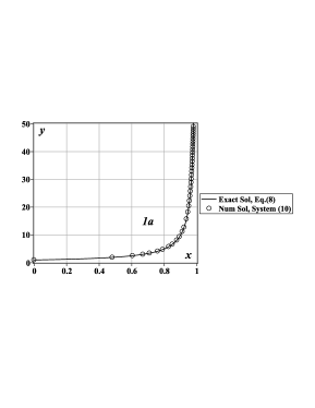
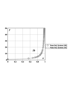
Figure 1: 1a — Exact solution (7) of the Cauchy problem (6) and numerical solution of system (8); 1b — numerical solutions of systems (8) and (13) ($a=1$ and $x_{*}=1$).

2.3 Solution method based on non-local transformations

Introducing a new non-local variable according to the formula,

$$\xi=\int^{x}_{x_{0}}g(x,y)\,dx,\quad\ y=y(x),$$ (10)

leads the Cauchy problem for one equation (1) to the equivalent problem for the autonomous system of equations

$$x^{\prime}_{\xi}=\frac{\mskip 1.0mu1\mskip 1.0mu}{\mskip 1.0mug(x,y)\mskip 1.0mu},\quad\ y^{\prime}_{\xi}=\frac{\mskip 1.0muf(x,y)\mskip 1.0mu}{\mskip 1.0mug(x,y)\mskip 1.0mu}\quad\ \ (\xi>0);\quad\ \ x(0)=x_{0},\quad y(0)=y_{0}.$$ (11)

Here, the function $g=g(x,y)$ has to satisfy the following conditions:

$$g>0\ \text{at}\ x\geq x_{0},\ y\geq y_{0};\quad\ g\to\infty\ \text{as}\ y\to\infty;\quad\ f/g=k\ \text{as}\ y\to\infty,$$ (12)

where $k=\text{const}>0$ (and the limiting case $k=\infty$ is also allowed); otherwise the function $g$ can be chosen rather arbitrarily.

From (10) and the second condition (12) it follows that $x^{\prime}_{\xi}\to 0$ as $\xi\to\infty$. The Cauchy problem (11) can be integrated numerically applying the Runge–Kutta method or other standard numerical methods.

Let us consider some possible selections of the function $g$ in the system (11).

$1^{\circ}$. We can take $g=\bigl{(}1+|f|^{s}\bigr{)}^{1/s}$ with $s>0$. In this case, $k=1$ in (12). For $s=2$, we get the method of the arc length transformation [2].

$2^{\circ}$. We can take $g=f/y$ that corresponds to $k=\infty$ in (12).

Example 2. For the test problem (6), in which $f=y^{2}$, we have $g=f/y=y$. By substituting these functions in (11), we arrive at the Cauchy problem

$$x^{\prime}_{\xi}=\frac{\mskip 1.0mu1\mskip 1.0mu}{\mskip 1.0muy\mskip 1.0mu},\quad\ y^{\prime}_{\xi}=y\quad\ \ (\xi>0);\quad\ \ x(0)=0,\quad y(0)=a.$$ (13)

The exact solution of this problem is written as follows:

$$x=\frac{\mskip 1.0mu1\mskip 1.0mu}{\mskip 1.0mua\mskip 1.0mu}\bigl{(}1-e^{-\xi}\bigr{)},\quad\ y=ae^{\xi}.$$ (14)

We can see that the unknown quantity $x=x(\xi)$ exponentially tend to the asymptotic values $x=x_{*}=1/a$ as $\xi\to\infty$.

The numerical solutions of the problems (8) and (13), obtained by the fourth-order Runge–Kutta method, are presented in Fig. 1b (for $a=1$ and the same stepsize $=0.2$). The numerical solutions are in a good agreement, but the method based on the non-local transformation with $g=t/y$ is more effective than the method based on a differential transformation.

3 Problems for second-order equations

3.1 Solution method based on a differential transformation

The Cauchy problem for the second-order differential equation has the form

$$y^{\prime\prime}_{xx}=f(x,y,y^{\prime}_{x})\quad(x>x_{0});\quad\ \ y(x_{0})=y_{0},\quad\ y^{\prime}_{x}(x_{0})=y_{1}.$$ (15)

Note that the exact solutions of equations of the form (15), which can be used for test problems with blow-up solutions, can be found, for example, in [7, 8].

Let $f(x,y,u)>0$ if $y>y_{0}\geq 0$ and $u>y_{1}\geq 0$, and the function $f$ increases quite rapidly as $y\to\infty$ (e.g. if $f$ does not depend on $y^{\prime}_{x}$, then $\displaystyle\lim_{y\to\infty}f/y=\infty$).

First, we represent ODE (15) as an equivalent system of equations

$$y^{\prime}_{x}=t,\quad\ y^{\prime\prime}_{xx}=f(x,y,t).$$ (16)

where $y=y(x)$ and $t=t(x)$ are unknown functions. Taking into account (16), we derive further a standard system of equations, assuming that $y=y(t)$ and $x=x(t)$. To do this, we differentiate the first equation in (16) with respect to $t$. We have $(y^{\prime}_{x})^{\prime}_{t}=1$. Taking into account the relations $y^{\prime}_{t}=tx^{\prime}_{t}$ (follows from the first equation of (16)) and $(y^{\prime}_{x})^{\prime}_{t}=y^{\prime\prime}_{xx}/t^{\prime}_{x}=x^{\prime}_{t}y^{\prime\prime}_{xx}$, we get further

$$x^{\prime}_{t}y^{\prime\prime}_{xx}=1.$$ (17)

If we eliminate the second derivative $y^{\prime\prime}_{xx}$ by using a second equation of (16), we obtain the first-order equation

$$x^{\prime}_{t}=\frac{\mskip 1.0mu1\mskip 1.0mu}{\mskip 1.0muf(x,y,t)\mskip 1.0mu}.$$ (18)

Considering further the relation $y^{\prime}_{t}=tx^{\prime}_{t}$, we transform (18) to the form

$$y^{\prime}_{t}=\frac{\mskip 1.0mut\mskip 1.0mu}{\mskip 1.0muf(x,y,t)\mskip 1.0mu}.$$ (19)

Equations (18) and (19) represent a system of coupled first-order equations with respect to functions $x=x(t)$ and $y=y(t)$. The system (18)–(19) should be defined with the initial conditions

$$x(t_{0})=x_{0},\quad y(t_{0})=y_{0},\quad t_{0}=y_{1}.$$ (20)

The Cauchy problem (18)–(20) can be integrated numerically applying the standard numerical methods [5, 6], without fear of blow-up solutions.

Remark 1.

Systems of equations (2) and (16) are particular cases of parametrically defined nonlinear differential equations, which are considered in [9, 10]. In [10], the general solutions of several parametrically defined ODEs were obtained via differential transformations, based on introducing a new independent variable $t=y^{\prime}_{x}$.

3.2 Examples of test problems and numerical solutions

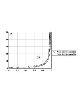
Figure 2: 2a — Exact solution (7) of the Cauchy problem (21) and numerical solution of system (22); 2b — numerical solutions of systems (22) and (25) ($a=1$ and $x_{*}=1$).

Example 3. Let us consider Cauchy problem

$$y^{\prime\prime}_{xx}=2y^{3}\quad\ (x>0),\quad\ y(0)=a,\quad\ y^{\prime}_{x}(0)=a^{2}.$$ (21)

The exact solution of this problem is defined by the formula (7).

Introducing a new variable $t=y^{\prime}_{x}$ in (21), we transform (21) to the Cauchy problem for the system of the first-order ODEs

$$x^{\prime}_{t}={\textstyle\frac{\mskip 1.0mu1\mskip 1.0mu}{\mskip 1.0mu2\mskip 1.0mu}}y^{-3},\ \ \ y^{\prime}_{t}={\textstyle\frac{\mskip 1.0mu1\mskip 1.0mu}{\mskip 1.0mu2\mskip 1.0mu}}ty^{-3}\ \ \ (t>t_{0});\quad\ x(t_{0})=0,\ \ \ y(t_{0})=a,\ \ \ t_{0}=a^{2},$$ (22)

which is a particular case of the problem (18)–(20) with $f=y^{2}$, $x_{0}=0$, and $y_{0}=a$. The exact solution of the problem (22) is given by the formulas (9).

Figure 2a shows a comparison of the exact solution (7) of the Cauchy problem for one equation (21) with the numerical solution of the system of equations (22), obtained by the fourth-order Runge–Kutta method (we have a good coincidence).

3.3 Solution method based on non-local transformations

First, equation (15) can be represented as a system of two equations

$$y^{\prime}_{x}=t,\quad\ t^{\prime}_{x}=f(x,y,t),$$

and then we introduce the non-local variable by the formula

$$\xi=\int^{x}_{x_{0}}g(x,y,t)\,dx,\quad\ y=y(x),\quad t=t(x).$$ (23)

As a result, the Cauchy problem (15) can be transformed to the following problem for an autonomous system of three equations:

$$\begin{gathered}x^{\prime}_{\xi}=\frac{\mskip 1.0mu1\mskip 1.0mu}{\mskip 1.0mug(x,y,t)\mskip 1.0mu},\quad\ y^{\prime}_{\xi}=\frac{\mskip 1.0mut\mskip 1.0mu}{\mskip 1.0mug(x,y,t)\mskip 1.0mu},\quad\ t^{\prime}_{\xi}=\frac{\mskip 1.0muf(x,y,t)\mskip 1.0mu}{\mskip 1.0mug(x,y,t)\mskip 1.0mu}\quad\ \ (\xi>0);\\ x(0)=x_{0},\quad\ y(0)=y_{0},\quad\ t(0)=y_{1}.\end{gathered}$$ (24)

For a suitable choice of the function $g=g(x,y,t)$ (not very restrictive conditions of the form (12) must be imposed on it), the Cauchy problem (24) can be numerically integrated applying the standard numerical methods [5, 6].

Let us consider some possible selections of the function $g$ in system (24).

$1^{\circ}$. We can take $g=\bigl{(}1+|t|^{s}+|f|^{s}\bigr{)}^{1/s}$ with $s>0$. The case $s=2$ corresponds to the method of the arc length transformation [2].

$2^{\circ}$. Also, we can take $g=f/y$, $g=f/t$, or $g=t/y$.

Example 4. For the test problem (21), in which $f=2y^{3}$, we put $g=t/y$. By substituting these functions in (24), we arrive at the Cauchy problem

$$x^{\prime}_{\xi}=y/t,\ \ y^{\prime}_{\xi}=y,\ \ t^{\prime}_{\xi}=2y^{4}/t\ \ (\xi>0);\ \ \ x(0)=0,\ \ y(0)=a,\ \ t(0)=a^{2}.$$ (25)

The exact solution of this problem is written as follows:

$$x=a^{-1}\bigl{(}1-e^{-\xi}\bigr{)},\quad\ y=ae^{\xi},\quad\ t=a^{2}e^{2\xi}.$$ (26)

We can see that the unknown quantity $x=x(\xi)$ exponentially tend to the asymptotic values $x=x_{*}=1/a$ as $\xi\to\infty$.

The numerical solutions of the problems (22) and (25), obtained by the fourth-order Runge–Kutta method, are presented in Fig. 2b (for $a=1$ and the same stepsize $=0.2$). The numerical solutions are in a good agreement, but the method based on the non-local transformation with $g=t/y$ is more effective than the method based on a differential transformation.

Remark 2.

The method described in Section 3.3 can be generalized to nonlinear ODEs of arbitrary order and systems of coupled ODEs.

References

[1]
G. Acosta, G. Durán, J. D. Rossi,
Computing, 2002, Vol. 68 343–373.
[2]
S. Moriguti, C. Okuno, R. Suekane, M. Iri, K. Takeuchi,
Ikiteiru Suugaku – Suuri Kougaku no Hatten (in Japanese),
Baifukan, Tokyo, 1979.
[3]
C. Hirota, K. Ozawa,
J. Comp. Appl. Math. 193 (2) (2006) 614–637.
[4]
P. G. Dlamini, M. Khumalo,
Math. Probl. Eng. 6 (2012) Art. ID 162034.
[5]
W. E. Schiesser.
Computational Mathematics in Engineering and Applied Science: ODEs, DAEs, and PDEs.
CRC Press, Boca Raton, 1994.
[6]
U. M. Ascher, L. R. Petzold,
Computer Methods for Ordinary Differential Equations and Differential-Algebraic Equations,
SIAM, 1998.
[7]
A. D. Polyanin, V. F. Zaitsev,
Handbook of Exact Solutions for Ordinary Differential Equations,
Chapman & Hall/CRC Press, Boca Raton, 2003.
[8]
N. A. Kudryashov.
Analytical Theory of Nonlinear Differential Equations (in Russian).
Institute of Computer Science, Moscow–Izhevsk, 2004.
[9]
A. D. Polyanin, A. I. Zhurov,
Appl. Math. Lett. 55 (2016) 72–80.
[10]
A. D. Polyanin, A. I. Zhurov,
Appl. Math. Lett. 64 (2017) 59–66.