Nikhef-2017-023
In Pursuit of New Physics with
Robert Fleischer a,b, Ruben Jaarsma a and Gilberto Tetlalmatzi-Xolocotzi a
aNikhef, Science Park 105, NL-1098 XG Amsterdam, Netherlands
bDepartment of Physics and Astronomy, Vrije Universiteit Amsterdam,
NL-1081 HV Amsterdam, Netherlands
Leptonic rare decays of mesons offer a powerful tool to search for physics beyond the Standard Model. The decay has been observed at the Large Hadron Collider and the first measurement of the effective lifetime of this channel was presented, in accordance with the Standard Model. On the other hand, and have received considerably less attention: while LHCb has recently reported a first upper limit of (95% C.L.) for the branching ratio, the upper bound (90% C.L.) for the branching ratio of was reported by CDF back in 2009. We discuss the current status of the interpretation of the measurement of , and explore the space for New-Physics effects in the other decays in a scenario assuming flavour-universal Wilson coefficients of the relevant four-fermion operators. While the New-Physics effects are then strongly suppressed by the ratio of the lepton masses in , they are hugely enhanced by in and may result in a branching ratio as large as about 5 times the one of , which is about a factor of 20 below the CDF bound; a similar feature arises in . Consequently, it would be most interesting to search for the channels at the LHC and Belle II, which may result in an unambiguous signal for physics beyond the Standard Model.
March 2017
1 Introduction
The decay belongs to the most interesting processes for testing the flavour sector of the Standard Model (SM). In this framework, emerges from quantum loop effects – penguin and box topologies – and is helicity suppressed. Consequently, this channel is strongly suppressed, and in the SM only about three out of one billion mesons decay into the final state. Another key feature of the decay is that the binding of the anti-bottom quark and the strange quark in the meson is described by a single non-perturbative parameter, the -meson decay constant [1]. In scenarios of New Physics (NP), may be affected by new particles entering the loop topologies or may even arise at the tree level.
For decades, experiments have searched for the decay [2]. It has been a highlight of run 1 of the Large Hadron Collider (LHC) that the mode could eventually be observed in a combined analysis by the CMS and LHCb collaborations [3]. The corresponding experimental branching ratio is consistent with the SM prediction.
In addition to the branching ratio, offers another observable [4]. It is accessible thanks to the sizeable difference between the decay widths of the mass eigenstates and is encoded in the effective lifetime. The LHCb collaboration has very recently reported a pioneering measurement of this observable, as well as the observation of in the analysis of their new data set collected at the ongoing run 2 of the LHC [5].
Furthermore, there is a CP-violating rate asymmetry which is generated through the interference between – mixing and decay processes [4, 6]. It would be very interesting to measure this observable. However, such an analysis requires tagging information on the decaying meson, thereby making it more challenging than the untagged effective lifetime measurement.
In the SM, the key difference of with respect to and is due to the different lepton masses. In the case of the former decay, the large mass effectively lifts the helicity suppression, while it gets much stronger for the latter process due to the small electron mass. Consequently, we have SM branching ratios at the and level, respectively, while the corresponding branching ratio takes a value at the level [1].
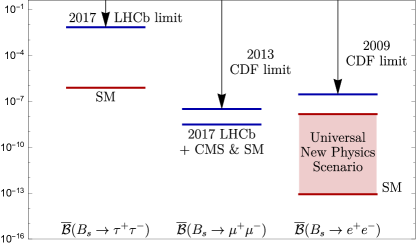
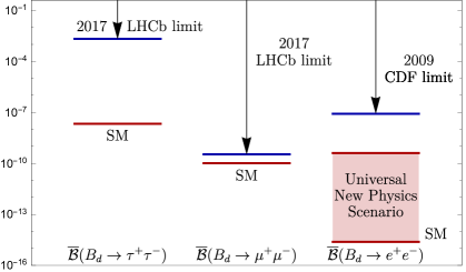
From the experimental point of view, the analysis of is challenging because of the reconstruction of the leptons. Nevertheless, LHCb has recently presented the first upper bound for this channel of (95% C.L.) [7]. The decay has received surprisingly little attention, both from the experimental and theoretical communities, and has so far essentially not played any role in the exploration of flavour physics. The most recent upper bound on the branching ratio of (90% C.L.) was obtained by the CDF collaboration back in 2009 [8]. We have illustrated this situation in Fig. 1.
We will have a fresh look at the search for NP effects with the and channels in view of the new LHCb data [5], complementing the recent study by Altmannshofer, Niehoff and Straub [9]. However, the main focus of our discussion will be on the and decays (as well as their counterparts), which were not considered in Ref. [9]. The utility of the decays with and in the final states for probing NP effects was addressed in the literature before, for instance, in Refs. [10, 11] and [12, 13], respectively. The current key question is how much space for NP effects is left in these channels by the currently available data, in particular for the experimentally established mode.
In order to explore this topic, which is in general very complex, and to illustrate possible NP effects, we consider a framework where the Wilson coefficients of the relevant four-fermion operators are flavour universal, i.e. do neither depend on the flavour of the decaying or mesons nor on the final-state leptons. We find that the corresponding NP effects are strongly suppressed in in this scenario. However, as the helicity suppression is lifted by new (pseudo)-scalar contributions, we may get a huge enhancement of the branching ratio of in this scenario, while still having the branching ratio of within the current experimental range. In particular, the branching ratio of may be enhanced to about 5 times the branching ratio, which is a factor of 20 below the CDF limit from 2009. Consequently, it would be most interesting to have a dedicated search for and , fully exploiting the physics potential of the LHC, where these decays will be interesting for ATLAS, CMS and LHCb, and the future Belle II experiment at KEK. In view of the theoretical cleanliness of these decays and the possible spectacular enhancement with respect to the SM, we may get an unambiguous signal for New Physics.
In Fig. 2, we have illustrated our NP analysis. The measured branching ratio of the channel allows us to constrain the corresponding short-distance functions, which are then converted into their counterparts for the and channels, having very different implications. The flowchart in Fig. 2 serves as a guideline for the following discussion.
The outline of this paper is as follows: we discuss the theoretical framework for our studies in Section 2. In Section 3, we have a closer look at the state-of-the-art picture following from the experimental results for the decays, while turning to the and modes in Sections 4 and 5, respectively. Finally, we summarize our conclusions in Section 6.
2 Theoretical Framework
2.1 Low-Energy Effective Hamiltonian
Leptonic rare decays of mesons () are described by the following low-energy effective Hamiltonian [1, 4, 9]:
| (1) |
where denotes the Fermi constant, are elements of the Cabibbo–Kobayashi–Maskawa (CKM) matrix, and is the QED fine structure constant. The heavy degrees of freedom have been integrated out and are described by the Wilson coefficients , and , which may depend both on the flavour of the quark and on the flavour of the final-state leptons . However, in the SM and NP scenarios with “Minimal Flavour Violation” (MFV) [14], the short-distance functions are flavour universal.

The Wilson coefficients are associated with the four-fermion operators
| (2) |
where denotes the -quark mass and
| (3) |
In the general Hamiltonian in Eq. (1), we have only kept operators which give non-vanishing contributions to decays. In the SM, only the operator is present with a real coefficient .
Concerning the impact of NP, the outstanding feature of the channels is their sensitivity to (pseudo)-scalar lepton densities entering the operators and , which have still largely unconstrained Wilson coefficients, thereby offering an interesting avenue for NP effects to enter. The decay amplitude has the following structure [1]:
| (4) |
where describes the helicity of the final-state leptons with and . The quantities
| (5) |
| (6) |
where and are the and masses, respectively, will play a key role in the following discussion. In general, the coefficients and have CP-violating phases and . In the SM, we obtain the simple relations
| (7) |
2.2 Decay Observables
The and mesons show the phenomenon of – mixing, which leads to time-dependent decay rates. Experiments actually measure the following time-integrated branching ratio [15]:
| (8) |
Here the time-dependent untagged rate, where no distinction is made between initially, i.e. at time , present or mesons, takes the following form [4, 9, 6]:
| (9) |
where the decay width difference enters through the parameter [16]
| (10) |
with denoting the lifetime. Using the quantities introduced above, the observable is given as follows [4, 6]:
| (11) |
Since it is challenging to determine the helicity of the final-state leptons experimentally, the rates in (9) are actually helicity-averaged. The observable takes the SM value
| (12) |
but is essentially unconstrained when allowing for NP effects [4, 6, 9].
In view of the sizeable , we have to properly distinguish between the time-integrated branching ratio measured at experiments and the “theoretical” branching ratio , which corresponds to the decay time . These two branching ratios can be converted into each other through the following relation [17]:
| (13) |
The physics information encoded in the effective lifetime
| (14) |
is equivalent to the observable [4], which can be determined with the help of
| (15) |
Moreover, allows us to convert the time-integrated branching ratio determined at experiments into the “theoretical” branching ratio with the help of the relation
| (16) |
where all quantities on the right-hand side can be measured [4, 17]. In the case of decays, takes a value at the level. Consequently, the corresponding observable is experimentally not accessible in the foreseeable future.
In addition to these untagged observables, there are also CP-violating asymmetries which would be very interesting to measure, providing insights into possible new sources for CP violation encoded in the Wilson coefficients [4, 6]. The experimental analysis of these observables would require tagging information, thereby making it more challenging than the exploration of . However, it would nevertheless be very interesting to make efforts in the super-high-precision era of physics to get also a handle on these quantities.
In order to search for NP effects by means of the branching ratio of the decays, it is useful to introduce the following ratio [4, 6]:
| (17) |
which takes by definition the SM value
| (18) |
Using the expressions given above yields
| (19) |
where denotes a possible NP contribution to the – mixing phase
| (20) |
Current experimental information from and decays with similar dynamics gives the following results [18, 16, 19]:
| (21) |
| (22) |
where we have used the SM value . Similar quantities can also be introduced for the decays, in analogy to the expressions given above.
2.3 Scenario for the New Physics Analysis
A first analysis of the interplay between and within specific models of physics beyond the SM was performed in Ref. [6], giving also a classification of various scenarios. In view of the new LHCb results for the mode, a very recent study was performed in Ref. [9], highlighting also the importance of measuring for the search and exploration of NP effects.
In order to illustrate NP effects, we shall consider a general scenario with no new sources of CP violation, i.e. real Wilson coefficients. This assumption could be explored with the help of the CP-violating observables discussed in Refs. [4, 6]. Moreover, we assume that we have flavour-universal Wilson coefficients, allowing us to introduce the notation
| (23) |
| (24) |
as well as
| (25) |
Using data for rare decays, the latter coefficient can be determined from experimental data (for a state-of-the-art analysis, see Ref. [20]). Data for modes allows us also to take a possible violation of Lepton Flavour Universality into account. As a working assumption, we shall use , which is consistent with the current rare -decay data within the uncertainties, and corresponds to a picture of NP entering only through new (pseudo)-scalar contributions, which is the key domain for the decays. We obtain then the following expressions:
| (26) |
| (27) |
which will serve as the basis for our following discussion of NP effects. In particular, we shall not assume any relation between the and coefficients, which typically arise in more general NP frameworks as well as in specific models [6, 13].
In Ref. [9], a scenario with heavy new degrees of freedom, which are linearly realized in the electroweak symmetry in the Higgs sector, and the feature of MFV was considered [13], including the Minimal Supersymmetric Standard Model (MSSM) with MFV violation. In the latter case, the coefficients , are suppressed by the mass ratio , and the relation holds. Moreover, these coefficients are proportional to the lepton mass (see also Refs. [6, 12]):
| (28) |
yielding
| (29) |
| (30) |
where does not depend on the lepton flavour . If we neglect the term under the square root in (30), both and are independent of the lepton mass in this scenario, implying that the ratios of branching ratios of the various decays are given as in the SM, up to corrections. In the case of the decays, these effects may have a sizeable impact, as we will discuss in Subsection 4.2.
The flavour-universal scenario introduced above offers an interesting general framework to explore NP effects in the and decays and to illustrate their potential impact. But before focusing on these modes, let us first discuss the picture for the channels following from the current data.
3 The Decays and
3.1 Experimental Status
Using the results of Ref. [1] and rescaling them to the updated parameters collected in Table 1, we obtain the following SM branching ratios:
| (31) |
| (32) |
On the experimental side, the LHCb collaboration has recently presented updated measurements of the and branching ratios [5]:
| (33) |
| (34) |
The CP-averaged signal for has a statistical significance of , while has a significance of , corresponding to (95% C.L.). These experimental results are consistent with the SM predictions within the uncertainties. In 2013, the CMS collaboration reported the following result [24]:
| (35) |
which corresponds to a signal with significance. The ATLAS collaboration presented the constraint in 2016 [25], which we give for comparison. The combination of the results in Eqs. (33) and (35) gives
| (36) |
where we have calculated the average by applying the procedure of the Particle Data Group (PDG) [22].
| Parameter | Value | Unit | Reference |
|---|---|---|---|
| GeV | [21] | ||
| GeV | [21] | ||
| GeV | [22] | ||
| GeV | [22] | ||
| GeV | [22] | ||
| GeV | [22] | ||
| GeV | [23] | ||
| GeV | [23] | ||
| [23] | |||
| [23] | |||
| [23] | |||
| ps | [16] | ||
| ps | [16] | ||
| GeV | [22] | ||
| GeV | [22] | ||
| [16] | |||
| [16] | |||
| [16] | |||
| [16] | |||
| [19] | |||
| [19] | |||
| [19] | |||
| [19] | |||
| [19] |
The LHCb collaboration has very recently reported a first measurement of the effective lifetime of the decay [5]:
| (37) |
Using the expression
| (38) |
with Eq. (12) and the numerical inputs in Table 1, we obtain the SM prediction
| (39) |
It agrees with the LHCb value, although the experimental uncertainties are too large to draw further conclusions. Using Eq. (15), we may convert Eq. (37) into
| (40) |
where the error is fully dominated by the huge uncertainty on the effective lifetime . As we have the model-independent relation
| (41) |
it will be crucial to improve the experimental precision for this observable in the future data taking at the LHC.
3.2 General Constraints on New Physics
Let us first have a look at the decay observables. Using Eqs. (31) and (36), we can determine the ratio from Eq. (17):
| (42) |
Assuming that we have no new CP-violating phases in and , as in the NP model introduced in Subsection 2.3, expression (19) reduces to
| (43) |
Using the experimental value of in Eq. (21) we get
| (44) |
which allows us to convert Eq. (42) into a circular band in the – plane.
The observable provides another constraint in this parameter space. Assuming real coefficients and , Eq. (11) yields
| (45) |
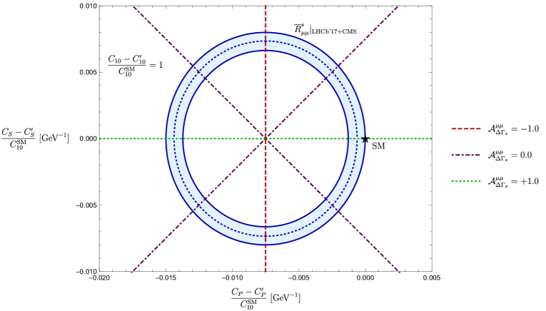
fixing a straight line in the – plane through the measured value of . Interestingly, as the NP phases phases enter as and in Eqs. (11) and (19), we cannot reveal minus signs of and , which correspond to , leading to terms of in the arguments of the relevant trigonometric functions, thereby leaving them unchanged. Consequently, and allow us to determine and up to discrete ambiguities:
| (46) |
| (47) |
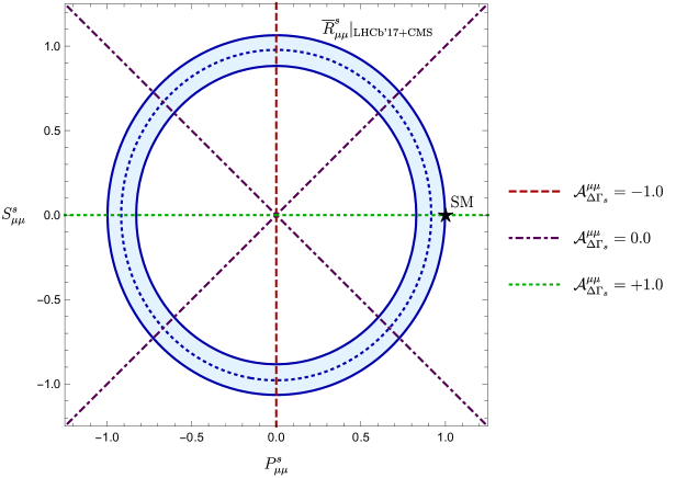
where we have also given the simplified expressions for . In Fig. 3, we illustrate the resulting situation in the – plane, showing both the circular band arising from the current experimental value of and the impact of a future measurement of the observable.
In order to test the SM with the decay, it is advantageous to consider the ratio of its branching ratio and the one of [26]. We obtain the following general expression:
| (48) | |||||
The CKM factor is required to utilize this ratio and has to be determined in a way that is robust with respect to the impact of NP effects. Assuming the unitarity of the CKM matrix, it can be extracted from the the length
| (49) |
of the Unitarity Triangle (UT) as . Here is the Wolfenstein parameter [27], and describes the apex of the UT in the complex plane [28]. Taking subleading corrections in into account and employing the UT side
| (50) |
we obtain
| (51) |
where is the angle between and the real axis.
Using pure tree decays of the kind [29, 30], can be determined in a theoretically clean way (for an overview, see [31]). The current experimental value is given as follows [19]:
| (52) |
In the future, thanks to Belle II [32] and the LHCb upgrade [33], the uncertainty for is expected to be reduced to the level.
Concerning the side, it can be determined with the help of and extracted from analyses of exclusive and inclusive semileptonic decays (for an overview, see the corresponding review in Ref. [22]). The current status can be summarized as
| (53) |
with the average
| (54) |
The determinations of and using pure tree decays are very robust with respect to NP effects. Consequently, they allow us to determine the ratio in Eq. (51) in a way that is also very robust concerning NP contributions, serving as the reference value for the analysis of Eq. (51). The current data with the average value of in Eq. (54) give
| (55) |
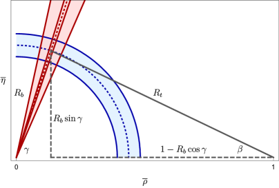
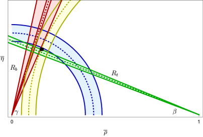
where the error may be reduced to in the Belle II and LHCb upgrade era. We have illustrated the resulting situation for the UT in the complex plane in the left panel of Fig. 4. Thanks to the specific shape of the UT, we observe that the uncertainty of is fully governed by , while the uncertainty of has a minor impact. Consequently, also the discrepancy between the inclusive and exclusive determinations in Eq. (53) has fortunately a negligible effect in this case. It is impressive to see the impact of the future extraction of , allowing a very precise determination of . For completeness, in the right panel of Fig. 4, we show other constraints in the – plane following from and the determination of the CKM angle through CP violation in decays, taking penguin effects into account [18]. For comprehensive analyses of the UT, the reader is referred to Refs. [19, 34, 35].
Using the CKM factor as determined through Eq. (51), we may convert the measured ratio of the branching ratios into the following parameter:
| (56) | |||||
which satisfies
| (57) |
For NP models with MFV, which are characterized by universal short-distance functions, we have – with excellent accuracy – also a value of around one. A tiny difference may arise from the following small differences [22]:
| (58) |
We shall return to this parameter within our general flavour-universal NP scenario in the next Subsection (see Eq. (68)).
The current data give
| (59) |
where the error is unfortunately too large to draw conclusions. At the end of the LHCb upgrade, corresponding to 50 fb-1 of integrated luminosity, LHCb expects to determine the ratio with a precision at the 35% level [33]. Assuming a future measurement of , which determines through Eq. (15), with a precision of [4] and a reduction in the uncertainty of to would yield
| (60) |
which would still not allow a stringent test in view of the significant uncertainty. We can straightforwardly generalize the observable defined in Eq. (56) to neutral decays with and leptons in the final state, as discussed below.
Should future measurements find a result for consistent with 1, thereby supporting the picture of the SM and models with MFV, we could extract the -breaking ratio of “bag” parameters describing – mixing from the following relation (see also Ref. [36]):
| (61) |
allowing – in principle – an interesting test of lattice QCD. An agreement between experiment and theory would also support the lattice QCD calculation of the decay constants , which are key inputs for the SM branching ratios. However, even in the LHCb upgrade era, we would only get a precision for Eq. (61) at the level of , while current lattice QCD calculations give the following picture [23]:
| (62) |
In order to determine the ratio of the bag parameters using Eq. (61) with the same relative error as the one achieved by the current lattice calculations in Eq. (62), the measurement of should reach the precision while having the error in the measurement of the effective lifetime as for the LHCb upgrade. In this future scenario, we would be able to achieve a precision of for the determination of the observable , which would be interesting territory to search for signals of physics from beyond the SM.
3.3 New Physics Benchmark Scenario
Let us now consider the situation in the general flavour-universal NP scenario introduced in Subsection 2.3, which is characterized by Eqs. (26) and (27), and assume that not only the ratio but also the observable has been measured. Using Eqs. (46) and (47), we may then determine the coefficients and , respectively, which allow us to extract the following ratios of short-distance coefficients:
| (63) |
| (64) |
Since we can only determine the absolute values of and , which are real in our scenario, we have also to allow for negative values. We illustrate the corresponding situation in Fig. 5. As the current measurement of in Eq. (40) does not yet provide a useful constraint, we vary this observable within its general range in Eq. (41), yielding
| (65) |
Once the observable has been measured with higher precision, these allowed ranges can be narrowed down correspondingly. In Ref. [13], constraints on similar coefficients were obtained.
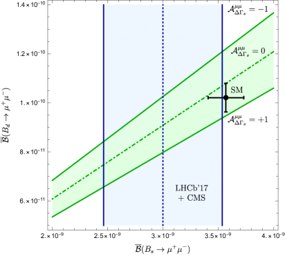
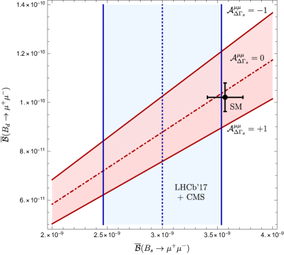
The coefficients in Eqs. (63) and (64), with the corresponding ranges in Eq. (65), may now be used to study correlations with the other decays. Following these lines, we obtain the correlation between the branching ratios of the and decays shown in Fig. 6, corresponding to the numerical range
| (66) |
with
| (67) |
which is consistent with the LHCb result in Eq. (34). Finally, we obtain
| (68) |
for the parameter introduced in Eq. (56). As expected from the discussion in the previous Subsection, this quantity shows a small difference from one due to the mass differences in Eq. (3.2) within the flavour-universal NP scenario. It will be very interesting to get much better measurements of the decay and to see whether they will be consistent with the picture given above.
4 The Decays and
4.1 Observables
As is evident from Eq. (9), the helicity suppression of the SM rates of the channels is essentially lifted through the large mass of the leptons. Within the SM, we obtain the following predictions:
| (69) |
| (70) |
In order to calculate these results, we have employed the analysis of Ref. [1], and have used the values of CKM and non-perturbative parameters given in Table 1.
It is experimentally very challenging to reconstruct the leptons, in particular in the environment of the LHC. Nevertheless, the LHCb collaboration has recently come up with the first experimental upper limits for the corresponding branching ratios [7]:
| (71) |
| (72) |
These results are in fact the first direct constraint for and the world’s best limit for .
The SM predictions for and take the same values as their counterparts:
| (73) |
4.2 New Physics Benchmark Scenario
Let us now have a look at the NP effects for the modes within the benchmark scenario introduced in Subsection 2.3. Here we obtain the following coefficients:
| (74) |
| (75) |
Consequently, the NP correction to and those proportional to and are strongly suppressed through the ratio of the muon and tau masses, which is given as follows [21]:
| (76) |
and yields
| (77) |
The impact of NP in the decay is very similar to its counterpart, with taking the same values as in Eq. (77). Introducing a parameter in analogy to Eq. (56), we obtain
| (78) |
In view of the challenges related to the reconstruction of the leptons, the NP effects arising in the general flavour-universal NP scenario cannot be distinguished from the SM case, unless there is unexpected experimental progress.
It is interesting to have a quick look at the picture in the MSSM with MFV described by Eqs. (29) and (30). As was pointed out in Ref. [9], the measured value of the ratio gives a twofold solutions for the parameter introduced in Eq. (29). We find
| (79) |
corresponding to the observables (as in the SM) and , respectively. These solutions give
| (80) |
and correspond to the branching ratios
| (81) |
respectively. We observe that the large -lepton mass has a significant impact on these quantities, in particular in the case .
5 The Decays and
5.1 Observables
The most recent SM predictions for the decays were given in Ref. [1]. Using the updated input parameters in Table 1, we obtain the following results:
| (82) |
| (83) |
The extremely small values of these branching ratios with respect to their counterparts arise from the helicity suppression due to the tiny electron mass, corresponding to an overall multiplicative factor in the expressions for . Consequently, within the SM, these decays appear to be out of reach from the experimental point of view, which seems to be the reason for the fact that these channels have so far essentially not played any role in the exploration of the quark-flavour sector.
Concerning the experimental picture, the CDF collaboration reported the following upper bounds ( C.L.) back in 2009 [8]:
| (84) |
| (85) |
Consequently, any attempt to measure the SM branching ratios for the rare decays and would require a future improvement by nearly six orders of magnitude. The LHC experiments have not yet reported any searches for these modes.
5.2 New Physics Benchmark Scenario
Let us now consider the flavour-universal NP scenario introduced in Subsection 3.3. In this framework, we obtain the following coefficients:
| (86) |
| (87) |
While we got a suppression of the NP effects in the decays through the large mass, (see (74) and (75)), we get now a huge enhancement thanks to the tiny electron mass [21]:
| (88) |
as the (pseudo)-scalar NP contributions lift the helicity suppression of the extremely small SM branching ratio.
The enhancement with respect to the SM value is characterized by
| (89) |
with
| (90) |
and
| (91) |
while
| (92) |
It is particularly interesting to consider the ratio between the and the branching ratios:
| (93) | |||||
where we used (see Eq. (44)) and neglected the effects associated with and the tiny mass ratio . As the decay constants and CKM matrix elements cancel in , this ratio is a theoretically clean quantity. Moreover, its measurement at the LHC is not affected by the ratio of fragmentation functions [37], which is an advantage from the experimental point of view.
It is instructive to consider a situation with and
| (94) |
which corresponds to a branching ratio as in the SM and is consistent with the current experimental situation. We obtain then
| (95) |
which yields
| (96) |
as varies between and while moving on the unit circle in the – plane. It is also interesting to note that would result in independently of the values of and on the unit circle, as can be seen in Eq. (93). These simple considerations illustrate nicely the possible spectacular enhancement of the branching ratio with respect to the SM prediction.
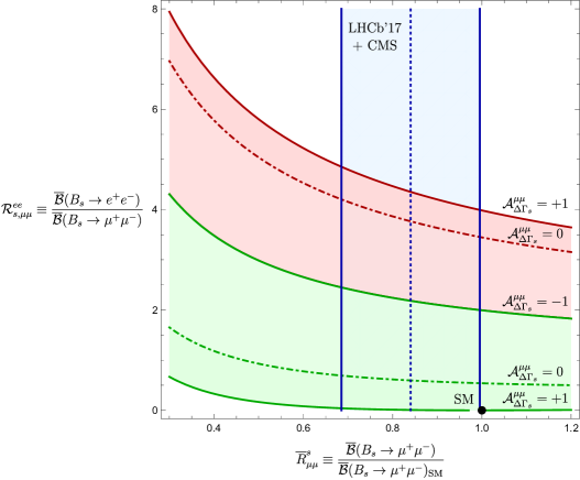
In Fig. 7, we put these considerations on a more quantitative ground, showing the allowed region for as a function of . We give also contours for various values of . If we vary this observable within the range in Eq. (41), we obtain
| (97) |
which is consistent with (96).
In the case of the branching ratio of the channel, we obtain uncertainties from the decay constant , CKM factors and the lifetime . The range in Eq. (97) corresponds to
| (98) |
with
| (99) |
showing an impressive lift of the helicity suppression with respect to the SM value in Eq. (82). The observable is just constrained within its general range .
The pattern of the NP effects in is very similar to the situation in its counterpart within the considered framework, yielding
| (100) |
In analogy to the case, it is instructive to have also a look at the MSSM with MFV, which is described by Eqs. (28–30) and the solutions in Eq. (79). In this framework, we get
| (101) |
where we have neglected tiny and corrections. Consequently, the ratio of the branching ratios is as in the SM, and we obtain from the measured branching ratio:
| (102) |
It will be very interesting to search for the decays, in particular in view of the exciting situation that the CDF upper bound from 2009 is only about a factor of 20 above the upper bound (98) in the flavour-universal NP scenario. Should the decays actually be observed with hugely enhanced branching ratios, the MSSM with MFV would be ruled out.
6 Conclusions
Leptonic rare decays of and mesons play an outstanding role for testing the SM. The main actors have so far been the and modes, where the former decay is now well established in the LHC data and first signals for the latter channel were reported. Very recently, LHCb has presented the first measurement of the effective lifetime of , and upper bounds for the and modes. The experimental constraint for is six orders of magnitude above the SM prediction, and was obtained by CDF in 2009.
We have given a state-of-the-art discussion of the interpretation of the data. However, the main focus was on the decays with tau leptons and electrons in the final state, addressing the question of how much space for NP effects is left by the current data, in particular the observation of . In order to explore this issue, which is in general very involved, we have considered a NP scenario as a benchmark with flavour-universal Wilson coefficients of the four-fermion operators, and assumed that NP enters through (pseudo)-scalar contributions, which is the key domain of the decays. We may then convert the experimental value of the branching ratio into predictions for the other channels. It will be important to significantly reduce the uncertainty of the measurement of the observable in the future, which will have an impact on the allowed regions for these channels.
In this scenario, we find that the NP effects are strongly suppressed by the mass ratio in the decays, thereby resulting in a picture which is essentially as in the SM. On the other hand, the NP effects are amplified in the channel due to the mass ratio . In this case, the helicity suppression is lifted by the new (pseudo)-scalar contributions, while the branching ratio of stays in the regime of the SM value, following from the current measurement of this channel. It is exciting to find values of the branching ratio about 5 times as large as the branching ratio, which is a factor of about 20 below the CDF limit. The ratio of the and branching ratios is a theoretically clean quantity, having also advantages from the experimental point of view.
Due to the helicity structure of possible NP contributions, is in general a very sensitive probe of physics beyond the SM with new (pseudo)-scalar contributions. As this decay has essentially not received any attention since the CDF analysis from 2009, it would be most interesting to search for in the LHC data, with the possibility of finding a signal which would give us unambiguous evidence for New Physics. In such a situation, the MSSM with MFV would be excluded.
In order to get the full picture, also and the corresponding modes should receive full attention at the LHC and the future Belle II experiments. We are excited to see new results – in particular searches for the decays – which may eventually open a window to the physics beyond the Standard Model.
Acknowledgements
This research has been supported by the Netherlands Foundation for Fundamental Research of Matter (FOM) programme 156, “Higgs as Probe and Portal”, and by the National Organisation for Scientific Research (NWO).
References
- [1] C. Bobeth, M. Gorbahn, T. Hermann, M. Misiak, E. Stamou and M. Steinhauser, Phys. Rev. Lett. 112 (2014) 101801 doi:10.1103/PhysRevLett.112.101801 [arXiv:1311.0903 [hep-ph]].
- [2] G. Borissov, R. Fleischer and M. H. Schune, Ann. Rev. Nucl. Part. Sci. 63 (2013) 205 doi:10.1146/annurev-nucl-102912-144527 [arXiv:1303.5575 [hep-ph]].
- [3] V. Khachatryan et al. [CMS and LHCb Collaborations], Nature 522 (2015) 68 doi:10.1038/nature14474 [arXiv:1411.4413 [hep-ex]].
- [4] K. De Bruyn, R. Fleischer, R. Knegjens, P. Koppenburg, M. Merk, A. Pellegrino and N. Tuning, Phys. Rev. Lett. 109 (2012) 041801 doi:10.1103/PhysRevLett.109.041801 [arXiv:1204.1737 [hep-ph]].
- [5] R. Aaij et al. [LHCb Collaboration], arXiv:1703.05747 [hep-ex].
- [6] A. J. Buras, R. Fleischer, J. Girrbach and R. Knegjens, JHEP 1307 (2013) 77 doi:10.1007/JHEP07(2013)077 [arXiv:1303.3820 [hep-ph]].
- [7] R. Aaij et al. [LHCb Collaboration], arXiv:1703.02508 [hep-ex].
- [8] T. Aaltonen et al. [CDF Collaboration], Phys. Rev. Lett. 102 (2009) 201801 doi:10.1103/PhysRevLett.102.201801 [arXiv:0901.3803 [hep-ex]].
- [9] W. Altmannshofer, C. Niehoff and D. M. Straub, arXiv:1702.05498 [hep-ph].
- [10] Y. Grossman, Z. Ligeti and E. Nardi, Phys. Rev. D 55, 2768 (1997) doi:10.1103/PhysRevD.55.2768 [hep-ph/9607473].
- [11] C. W. Chiang, X. G. He, F. Ye and X. B. Yuan, arXiv:1703.06289 [hep-ph].
- [12] C. Bobeth, G. Hiller and G. Piranishvili, JHEP 0712, 040 (2007) doi:10.1088/1126-6708/2007/12/040 [arXiv:0709.4174 [hep-ph]].
- [13] R. Alonso, B. Grinstein and J. Martin Camalich, Phys. Rev. Lett. 113 (2014) 241802 doi:10.1103/PhysRevLett.113.241802 [arXiv:1407.7044 [hep-ph]].
- [14] G. D’Ambrosio, G. F. Giudice, G. Isidori and A. Strumia, Nucl. Phys. B 645 (2002) 155 doi:10.1016/S0550-3213(02)00836-2 [hep-ph/0207036].
- [15] I. Dunietz, R. Fleischer and U. Nierste, Phys. Rev. D 63 (2001) 114015 doi:10.1103/PhysRevD.63.114015 [hep-ph/0012219].
- [16] Y. Amhis et al. [Heavy Flavor Averaging Group], arXiv:1612.07233 [hep-ex] and online update at http://www.slac.stanford.edu/xorg/hfag/.
- [17] K. De Bruyn, R. Fleischer, R. Knegjens, P. Koppenburg, M. Merk and N. Tuning, Phys. Rev. D 86 (2012) 014027 doi:10.1103/PhysRevD.86.014027 [arXiv:1204.1735 [hep-ph]].
- [18] K. De Bruyn and R. Fleischer, JHEP 1503 (2015) 145 doi:10.1007/JHEP03(2015)145 [arXiv:1412.6834 [hep-ph]].
- [19] J. Charles et al., Phys. Rev. D 91 (2015) no.7, 073007 doi:10.1103/PhysRevD.91.073007 [arXiv:1501.05013 [hep-ph]]; for updates, see http://ckmfitter.in2p3.fr.
- [20] W. Altmannshofer, C. Niehoff, P. Stangl and D. M. Straub, arXiv:1703.09189 [hep-ph].
- [21] P. J. Mohr, D. B. Newell and B. N. Taylor, Rev. Mod. Phys. 88 (2016) no.3, 035009 doi: 10.1103/RevModPhys.88.035009 [physics.atom-ph/1507.07956] http://physics.nist.gov/cuu/Constants/.
- [22] 2016 Review of Particle Physics. C. Patrignani et al.(Particle Data Group), Chin. Phys. C, 40 (2016) 100001.
- [23] S. Aoki et al., Review of lattice results concerning low-energy particle physics, [hep-lat/1607.00299].
- [24] S. Chatrchyan et al. [CMS Collaboration], Phys. Rev. Lett. 111 (2013) 101804 doi:10.1103/PhysRevLett.111.101804 [arXiv:1307.5025 [hep-ex]].
- [25] M. Aaboud et al. [ATLAS Collaboration], Eur. Phys. J. C 76 (2016) no.9, 513 doi:10.1140/epjc/s10052-016-4338-8 [arXiv:1604.04263 [hep-ex]].
- [26] A. J. Buras and R. Fleischer, Adv. Ser. Direct. High Energy Phys. 15 (1998) 65 [hep-ph/9704376].
- [27] L. Wolfenstein, Phys. Rev. Lett. 51 (1983) 1945.
- [28] A. J. Buras, M. E. Lautenbacher and G. Ostermaier, Phys. Rev. D 50 (1994) 3433 doi:10.1103/PhysRevD.50.3433 [hep-ph/9403384].
- [29] M. Gronau and D. Wyler, Phys. Lett. B 265 (1991) 172. doi:10.1016/0370-2693(91)90034-N
- [30] D. Atwood, I. Dunietz and A. Soni, Phys. Rev. Lett. 78 (1997) 3257 doi:10.1103/PhysRevLett.78.3257 [hep-ph/9612433]; Phys. Rev. D 63 (2001) 036005 doi:10.1103/PhysRevD.63.036005 [hep-ph/0008090].
- [31] R. Fleischer and S. Ricciardi, proceedings of the 6th International Workshop on the CKM Unitarity Triangle (CKM 2010) [arXiv:1104.4029 [hep-ph]].
- [32] T. Abe et al. [Belle-II Collaboration], arXiv:1011.0352 [physics.ins-det].
- [33] R. Aaij et al. [LHCb Collaboration], Eur. Phys. J. C 73 (2013) 2373 doi:10.1140/epjc/s10052-013-2373-2 [arXiv:1208.3355 [hep-ex]].
- [34] A. Bevan et al., arXiv:1411.7233 [hep-ph]; for updates, see http://www.utfit.org.
- [35] M. Blanke and A. J. Buras, Eur. Phys. J. C 76 (2016) no. 4, 197 doi:10.1140/epjc/s10052-016-4044-6 [arXiv:1602.04020 [hep-ph]].
- [36] A. J. Buras, Phys. Lett. B 566 (2003) 115 doi:10.1016/S0370-2693(03)00561-6 [hep-ph/0303060].
- [37] R. Fleischer, N. Serra and N. Tuning, Phys. Rev. D 82 (2010) 034038 doi:10.1103/PhysRevD.82.034038 [arXiv:1004.3982 [hep-ph]].