Extraction of partonic transverse momentum distributions from semi-inclusive deep-inelastic scattering, Drell–Yan and Z-boson production
Abstract
We present an extraction of unpolarized partonic transverse momentum distributions (TMDs) from a simultaneous fit of available data measured in semi-inclusive deep-inelastic scattering, Drell–Yan and boson production. To connect data at different scales, we use TMD evolution at next-to-leading logarithmic accuracy. The analysis is restricted to the low-transverse-momentum region, with no matching to fixed-order calculations at high transverse momentum. We introduce specific choices to deal with TMD evolution at low scales, of the order of 1 GeV2. This could be considered as a first attempt at a global fit of TMDs.
pacs:
13.60.Le, 13.87.Fh,14.20.DhI Introduction
Parton distribution functions describe the internal structure of the nucleon in terms of its elementary constituents (quarks and gluons). They cannot be easily computed from first principles, because they require the ability to carry out Quantum Chromodynamics (QCD) calculations in its nonperturbative regime. Many experimental observables in hard scattering experiments involving hadrons are related to parton distribution functions (PDFs) and fragmentation functions (FFs), in a way that is specified by factorization theorems (see, e.g., Refs. Collins et al. (1989); Collins (2013)). These theorems also elucidate the universality properties of PDFs and FFs (i.e., the fact that they are the same in different processes) and their evolution equations (i.e., how they get modified by the change in the hard scale of the process). Availability of measurements of different processes in different experiments makes it possible to test factorization theorems and extract PDFs and FFs through so-called global fits. On the other side, the knowledge of PDFs and FFs allows us to make predictions for other hard hadronic processes. These general statements apply equally well to standard collinear PDFs and FFs and to transverse-momentum-dependent parton distribution functions (TMD PDFs) and fragmentation functions (TMD FFs). Collinear PDFs describe the distribution of partons integrated over all components of partonic momentum except the one collinear to the parent hadron; hence, collinear PDFs are functions of the parton longitudinal momentum fraction . TMD PDFs (or TMDs for short) include also the dependence on the transverse momentum . They can be interpreted as three-dimensional generalizations of collinear PDFs. Similar arguments apply to collinear FFs and TMD FFs Angeles-Martinez et al. (2015).
There are several differences between collinear and TMD distributions. From the formal point of view, factorization theorems for the two types of functions are different, implying also different universality properties and evolution equations Rogers (2016). From the experimental point of view, observables related to TMDs require the measurement of some transverse momentum component much smaller than the hard scale of the process Bacchetta (2016); Radici (2016). For instance, Deep-Inelastic Scattering (DIS) is characterized by a hard scale represented by the 4-momentum squared of the virtual photon (). In inclusive DIS this is the only scale of the process, and only collinear PDFs and FFs can be accessed. In semi-inclusive DIS (SIDIS) also the transverse momentum of the outgoing hadron () can be measured Mulders and Tangerman (1996); Bacchetta et al. (2007). If , TMD factorization can be applied and the process is sensitive to TMDs Collins (2013).
If polarization is taken into account, several TMDs can be introduced Mulders and Tangerman (1996); Boer and Mulders (1998); Bacchetta and Mulders (2000); Mulders and Rodrigues (2001); Boer et al. (2016). Attempts to extract some of them have already been presented in the past Bacchetta and Radici (2011); Anselmino et al. (2012); Echevarria et al. (2014); Anselmino et al. (2016); Lu and Schmidt (2010); Barone et al. (2015); Lefky and Prokudin (2015); Anselmino et al. (2013); Kang et al. (2016). In this work, we focus on the simplest ones, i.e., the unpolarized TMD PDF and the unpolarized TMD FF , where is the fractional energy carried by the detected hadron , is the transverse momentum of the parton with respect to the parent hadron, and is the transverse momentum of the produced hadron with respect to the parent parton. Despite their simplicity, the phenomenology of these unpolarized TMDs presents several challenges Signori (2016a): the choice of a functional form for the nonperturbative components of TMDs, the inclusion of a possible dependence on partonic flavor Signori et al. (2013), the implementation of TMD evolution Bacchetta et al. (2015); Rogers (2016), the matching to fixed-order calculations in collinear factorization Collins et al. (2016).
We take into consideration three kinds of processes: SIDIS, Drell–Yan processes (DY) and the production of bosons. To date, they represent all possible processes where experimental information is available for unpolarized TMD extractions. The only important process currently missing is electron-positron annihilation, which is particularly important for the determination of TMD FFs Bacchetta et al. (2015). This work can therefore be considered as the first attempt at a global fit of TMDs.
The paper is organized as follows. In Sec. II, the general formalism for TMDs in SIDIS, DY processes, and Z production is briefly outlined, including a description of the assumptions and approximations in the phenomenological implementation of TMD evolution equations. In Sec. III, the criteria for selecting the data analyzed in the fit are summarized and commented. In Sec. IV, the results of our global fit are presented and discussed. In Sec. V, we summarize the results and present an outlook for future improvements.
II Formalism
II.1 Semi-inclusive DIS
In one-particle SIDIS, a lepton with momentum scatters off a hadron target with mass and momentum . In the final state, the scattered lepton momentum is measured together with one hadron with mass and momentum . The corresponding reaction formula is
| (1) |
The space-like momentum transfer is , with . We introduce the usual invariants
| (2) |
The available data refer to SIDIS hadron multiplicities, namely to the differential number of hadrons produced per corresponding inclusive DIS event. In terms of cross sections, we define the multiplicities as
| (3) |
where is the differential cross section for the SIDIS process and is the corresponding inclusive one, and where is the component of transverse to (we follow here the notation suggested in Ref. Boer et al. (2011a)). In the single-photon-exchange approximation, the multiplicities can be written as ratios of structure functions (see Ref. Bacchetta et al. (2007) for details):
| (4) |
where
| (5) |
In the numerator of Eq. (4) the structure function corresponds to a lepton with polarization scattering on a target with polarization by exchanging a virtual photon in a polarization state . In the denominator, only the photon polarization is explicitly written (, ), as usually done in the literature.
The semi-inclusive cross section can be expressed in a factorized form in terms of TMDs only in the kinematic limits and . In these limits, the structure function of Eq. (4) can be neglected Bacchetta et al. (2008a). The structure function in the denominator contains contributions involving powers of the strong coupling constant at an order that goes beyond the level reached in this analysis; hence, it will be consistently neglected (for measurements and estimates of the structure function see, e.g., Refs. Chekanov et al. (2009); Andreev et al. (2014) and references therein).
To express the structure functions in terms of TMD PDFs and FFs, we rely on the factorized formula for SIDIS Collins and Soper (1981); Collins et al. (1985); Ji and Yuan (2002); Ji et al. (2005); Collins (2013); Aybat and Rogers (2011); Echevarria et al. (2012, 2013); Collins and Rogers (2013) (see Fig. 1 for a graphical representation of the involved transverse momenta):
| (6) | ||||
Here, is the hard scattering part; is the TMD PDF of unpolarized partons with flavor in an unpolarized proton, carrying longitudinal momentum fraction and transverse momentum . The is the TMD FF describing the fragmentation of an unpolarized parton with flavor into an unpolarized hadron carrying longitudinal momentum fraction and transverse momentum (see Fig. 1). TMDs generally depend on two energy scales Collins (2013), which enter via the renormalization of ultraviolet and rapidity divergencies. In this work we choose them to be equal and set them to . The term is introduced to ensure a matching to the perturbative fixed-order calculations at higher transverse momenta.

In our analysis, we neglect any correction of the order of or higher to Eq. (6). At large this is well justified. However, fixed-target DIS experiments typically collect a large amount of data at relatively low values, where these assumptions should be all tested in future studies. The reliability of the theoretical description of SIDIS at low has been recently discussed in Refs. Boglione et al. (2017); Moffat et al. (2017).
Eq. (6) can be expanded in powers of . In the present analysis, we will consider only the terms at order . In this case and . However, perturbative corrections include large logarithms , so that . In the present analysis, we will take into account all leading and Next-to-Leading Logarithms (NLL).111We remark that formulas at NNLL are available in the literature Echevarria et al. (2016).
In these approximations ( and NLL), only the first term in Eq. (6) is relevant (often in the literature this has been called term). We expect this term to provide a good description of the structure function only in the region where . It can happen that , defined in the standard way (see, e.g., Ref. Collins et al. (1985)), gives large contributions also in this region, but it is admissible to redefine it in order to avoid this problem Collins et al. (2016). We leave a detailed treatment of the matching to the high region to future investigations.
To the purpose of applying TMD evolution equations, we need to calculate the Fourier transform of the part of Eq. (6) involving TMDs. The structure function thus reduces to
| (7) |
where we introduced the Fourier transforms of the TMD PDF and FF according to
| (8) | ||||
| (9) |
II.2 Drell–Yan and Z production
In a Drell–Yan process, two hadrons and with momenta and collide at a center-of-mass energy squared and produce a virtual photon or a boson plus hadrons. The boson decays into a lepton-antilepton pair. The reaction formula is
| (10) |
The invariant mass of the virtual photon is with . We introduce the rapidity of the virtual photon/Z boson
| (11) |
where the direction is defined along the momentum of hadron A (see Fig. 2).
The cross section can be written in terms of structure functions Boer and Vogelsang (2006); Arnold et al. (2009). For our purposes, we need the unpolarized cross section integrated over and over the azimuthal angle of the virtual photon,
| (12) |
The elementary cross sections are
| (13) |
where is Weinberg’s angle, is the mass of the boson, and is the branching ratio for the boson decay in two leptons. We adopted the narrow-width approximation, i.e., we neglect contributions for . We used the values , GeV, and Patrignani et al. (2016). Similarly to the SIDIS case, in the kinematic limit the structure function can be neglected (for measurement and estimates of this structure function see, e.g., Ref. Lambertsen and Vogelsang (2016) and references therein).
The longitudinal momentum fractions of the annihilating quarks can be written in terms of rapidity in the following way
| (14) |
Some experiments use the variable , which is connected to the other variables by the following relations
| (15) |
The structure function can be written as (see Fig. 2 for a graphical representation of the involved transverse momenta)
| (16) | ||||

As in the SIDIS case, in our analysis we neglect the term and we consider the hard coefficients only up to leading order in the couplings, i.e.,
| (17) |
where222We remind the reader that the value of weak isospin is equal to for , , and for , , .
| (18) |
The structure function can be conveniently expressed as a Fourier transform of the right-hand side of Eq. (16) as
| (19) |
II.3 TMDs and their evolution
Evolution equations quantitatively describe the connection between different values for the energy scales. In the following we will set their initial values to and their final values as , so that only and need to be specified in a TMD distribution. Following the formalism of Refs. Collins (2013); Aybat and Rogers (2011), the unpolarized TMD distribution and fragmentation functions in configuration space for a parton with flavor at a certain scale can be written as
| (20) | ||||
| (21) |
We choose the scale to be
| (22) |
where is the Euler constant and
| (23) |
This variable replaces the simple dependence upon in the perturbative parts of the TMD definitions of Eqs. (20), (21). In fact, at large these parts are no longer reliable. Therefore, the is chosen to saturate on the maximum value , as suggested by the CSS formalism Collins (2013); Aybat and Rogers (2011). On the other hand, at small the TMD formalism is not valid and should be matched to the fixed-order collinear calculations. The way the matching is implemented is not unique. In any case, the TMD contribution can be arbitrarily modified at small . In our approach, we choose to saturate at the minimum value . With the appropriate choices, for the Sudakov exponent vanishes, as it should Parisi and Petronzio (1979); Altarelli et al. (1984). Our choice partially corresponds to modifying the resummed logarithms as in Ref. Bozzi et al. (2011) and to other similar modifications proposed in the literature Boer and den Dunnen (2014); Collins et al. (2016). One advantage of these kind of prescriptions is that by integrating over the impact parameter , the collinear expression for the cross section in terms of collinear PDFs is recovered, at least at leading order Collins et al. (2016). We remind the reader that there are different schemes available to deal with the high- region, such as the the so-called “complex- prescription” Laenen et al. (2000) or an extrapolation of the perturbative small- calculation to the large region based on dynamical power corrections Qiu and Zhang (2001).
The values of and could be regarded as arbitrary scales separating perturbative from nonperturbative regimes. We choose to fix them to the values
| (24) |
The motivations are the following:
-
•
with the above choices, the scale is constrained between 1 GeV and , so that the collinear PDFs are never computed at a scale lower than 1 GeV and the lower limit of the integrals contained in the definition of the perturbative Sudakov factor (see Eq. (30)) can never become larger than the upper limit;
-
•
at GeV, and there are no evolution effects; the TMD is simply given by the corresponding collinear function multiplied by a nonperturbative contribution depending on (plus possible corrections of order from the Wilson coefficients).
At NLL accuracy, for our choice of scales . Similarly, the and are perturbatively calculable Wilson coefficients for the TMD distribution and fragmentation functions, respectively. They are convoluted with the corresponding collinear functions according to
| (25) | ||||
| (26) |
In the present analysis, we consider only the leading-order term in the expansion for and , i.e.,
| (27) |
As a consequence of the choices we made, the expression for the evolved TMD functions reduces to
| (28) | ||||
| (29) |
The Sudakov exponent can be written as
| (30) |
where the functions and have a perturbative expansions of the form
| (31) |
To NLL accuracy, we need the following terms Davies and Stirling (1984); Collins et al. (1985)
| (32) |
We use the approximate analytic expression for at NLO with the 340 MeV, 296 MeV, 214 MeV for three, four, five flavors, respectively, corresponding to a value of . We fix the flavor thresholds at GeV and GeV. The integration of the Sudakov exponent in Eq. (30) can be done analytically (for the complete expressions see, e.g., Refs. Frixione et al. (1999); Bozzi et al. (2006); Echevarria et al. (2013)).
Following Refs. Nadolsky et al. (2000); Landry et al. (2003); Konychev and Nadolsky (2006), for the nonperturbative Sudakov factor we make the traditional choice
| (33) |
with a free parameter. Recently, several alternative forms have been proposed Aidala et al. (2014); Collins and Rogers (2015). Also, recent theoretical studies aimed at calculating this term using nonperturbative methods Scimemi and Vladimirov (2017). All these choices should be tested in future studies. In Ref. D’Alesio et al. (2014a), a good agreement with data was achieved even without this term, but this is not possible when including data at low .
In this analysis, for the collinear PDFs we adopt the GJR08FFnloE set Gluck et al. (2008) through the LHAPDF library Buckley et al. (2015), and for the collinear fragmentation functions the DSS14 NLO set for pions de Florian et al. (2015) and the DSS07 NLO set for kaons de Florian et al. (2007).333After the completion of our analysis, a new set of kaon fragmentation function was presented in Ref. de Florian et al. (2017). We will comment on the use of other PDF sets in Sec. IV.3.
We parametrize the intrinsic nonperturbative parts of the TMDs in the following ways
| (34) | ||||
| (35) |
After performing the anti-Fourier transform, the and in momentum space correspond to
| (36) | ||||
| (37) |
The TMD PDF at the starting scale is therefore a normalized sum of a Gaussian with variance and the same Gaussian weighted by a factor . The TMD FF at the starting scale is a normalized sum of a Gaussian with variance and a second Gaussian with variance weighted by a factor . The choice of this particular functional forms is motivated by model calculations: the weighted Gaussian in the TMD PDF could arise from the presence of components of the quark wave function with angular momentum Bacchetta et al. (2008b); Pasquini et al. (2008); Avakian et al. (2010); Bacchetta et al. (2010); Burkardt and Pasquini (2016). Similar features occur in models of fragmentation functions Bacchetta et al. (2002); Bacchetta et al. (2008b); Matevosyan et al. (2012).
The Gaussian width of the TMD distributions may depend on the parton flavor Signori et al. (2013); Matevosyan et al. (2012); Schweitzer et al. (2013). In the present analysis, however, we assume they are flavor independent. The justification for this choice is that most of the data we are considering are not sufficiently sensitive to flavor differences, leading to unclear results. We will devote attention to this issue in further studies.
Finally, we assume that the Gaussian width of the TMD depends on the fractional longitudinal momentum according to
| (38) |
where and with , are free parameters. Similarly, for fragmentation functions we have
| (39) |
where and with are free parameters.
III Data analysis
The main goals of our work are to extract information about intrinsic transverse momenta, to study the evolution of TMD parton distributions and fragmentation functions over a large enough range of energy, and to test their universality among different processes. To achieve this we included measurements taken from SIDIS, Drell–Yan and boson production from different experimental collaborations at different energy scales. In this chapter we describe the data sets considered for each process and the applied kinematic cuts.
Tab. 1 refers to the data sets for SIDIS off proton target (Hermes experiment) and presents their kinematic ranges. The same holds for Tab. 2, Tab. 3, Tab. 4 for SIDIS off deuteron (Hermes and Compass experiments), Drell–Yan events at low energy and boson production respectively. If not specified otherwise, the theoretical formulas are computed at the average values of the kinematic variables in each bin.
III.1 Semi-inclusive DIS data
The SIDIS data are taken from Hermes Airapetian et al. (2013) and Compass Adolph et al. (2013) experiments. Both data sets have already been analyzed in previous works, e.g., Refs. Signori et al. (2013); Anselmino et al. (2014), however they have never been fitted together, including also the contributions deriving from TMD evolution.
The application of the TMD formalism to SIDIS depends on the capability of identifying the current fragmentation region. This task has been recently discussed in Ref. Boglione et al. (2017), where the authors point out a possible overlap among different fragmentation regions when the hard scale is sufficiently low. In this paper we do not tackle this problem and we leave it to future studies. As described in Tabs. 1 and 2, we identify the current fragmentation region operating a cut on only, namely .
Another requirement for the applicability of TMD factorization is the presence of two separate scales in the process. In SIDIS, those are the and , which should satisfy the condition , or more precisely . We implement this condition by imposing GeV. With this choice, is always smaller than , but in a few bins (at low and ) may become larger than . The applicability of TMD factorization in this case could be questioned. However, as we will explain further in Sec. IV.3, we can obtain a fit that can describe a wide region of and can also perform very well in a restricted region, where TMD factorization certainly holds.
III.1.1 Hermes data
Hermes hadron multiplicities are measured in a fixed target experiment, colliding a GeV lepton beam on a hydrogen () or deuterium () gas target, for a total of 2688 points. These are grouped in bins of with the average values of ranging from about to . The collinear energy fraction in Eq. (2) ranges in . The transverse momentum of the detected hadron satisfies . The peculiarity of Hermes SIDIS experiment lies in the ability of its detector to distinguish between pions and kaons in the final state, in addition to determining their momenta and charges. We consider eight different combinations of target () and detected charged hadron ( ). The Hermes collaboration published two distinct sets, characterized by the inclusion or subtraction of the vector meson contribution. In our work we considered only the data set where this contribution has been subtracted.
III.1.2 Compass data
The Compass collaboration extracted multiplicities for charge-separated but unidentified hadrons produced in SIDIS off a deuteron () target Adolph et al. (2013). The number of data points is an order of magnitude higher compared to the Hermes experiment. The data are organized in multidimensional bins of , they cover a range in from about to and the interval . The multiplicities published by Compass are affected by normalization errors (see the erratum to Ref. Adolph et al. (2013)). In order to avoid this issue, we divide the data in each bin in () by the data point with the lowest in the bin. As a result, we define the normalized multiplicity as
| (41) |
where the multiplicity is defined in Eq. (3). When fitting normalized multiplicities, the first data point of each bin is considered as a fixed constraint and excluded from the degrees of freedom.
III.2 Low-energy Drell–Yan data
We analyze Drell–Yan events collected by fixed-target experiments at low-energy. These data sets have been considered also in previous works, e.g., in Ref. Landry et al. (2001, 2003); Konychev and Nadolsky (2006); D’Alesio et al. (2014b). We used data sets from the E288 experiment Ito et al. (1981), which measured the invariant dimuon cross section for the production of pairs from the collision of a proton beam with a fixed target, either composed of Cu or Pt. The measurements were performed using proton incident energies of , and GeV, producing three different data sets. Their respective center of mass energies are GeV. We also included the set of measurements from E605 Moreno et al. (1991), extracted from the collision of a proton beam with an energy of GeV ( GeV) on a copper fixed target .
The explored values are higher compared to the SIDIS case, as can be seen in Tab. 3. E288 provides data at fixed rapidity, whereas E605 provides data at fixed . We can apply TMD factorization if , where is the transverse momentum of the intermediate electroweak boson, reconstructed from the kinematics of the final state leptons. We choose GeV. As suggested in Ref. Ito et al. (1981), we consider the target nuclei as an incoherent ensemble composed by protons and by neutrons.
As we already observed, results from E288 and E605 experiments are reported as ; this variable is related to the differential cross section of Eq. (12) in the following way:
| (42) |
where is the polar angle of and the third term is the average over . Therefore, the invariant dimuon cross section can be obtained from Eq. (12) integrating over and adding a factor to the result
| (43) |
Numerically we checked that integrating in only the prefactor (see Eq. (13)) introduces only a negligible error in the theoretical estimates. We also assume that does not change within the experimental bin. Therefore, for Drell–Yan we obtain
| (44) |
where are the lower and upper values in the experimental bin.
III.3 Z-boson production data
In order to reach higher and values, we also consider boson production in collider experiments at Tevatron. We analyze data from CDF and D0, collected during Tevatron Run I Affolder et al. (2000); Abbott et al. (2000) at and Run II Aaltonen et al. (2012); Abazov et al. (2008) at . CDF and D0 collaborations studied the differential cross section for the production of an pair from collision through an intermediate vector boson, namely .
The invariant mass distribution peaks at the -pole, , while the transverse momentum of the exchanged ranges in . We use the same kinematic cut applied to Drell–Yan events: GeV GeV, since is fixed to .
The observable measured in CDF and D0 is
| (45) |
apart from the case of D0 Run II, for which the published data refer to . In order to work with the same observable, we multiply the D0 Run II data by the total cross section of the process Abulencia et al. (2007). In this case, we add in quadrature the uncertainties of the total cross section and of the published data.
We normalize our functional form with the factors listed in Tab. 4. These are the same normalization factors used in Ref. D’Alesio et al. (2014b), computed by comparing the experimental total cross section with the theoretical results based on the code of Ref. Catani et al. (2009). These factors are not precisely consistent with our formulas. In fact, as we will discuss in Sec. IV.3 a 5% increase in these factors would improve the agreement with data, without affecting the TMD parameters.
| Hermes | Hermes | Hermes | Hermes | |
| Reference | Airapetian et al. (2013) | |||
| Cuts | ||||
| GeV | ||||
| Points | 190 | 190 | 189 | 187 |
| Max. | ||||
| range | ||||
| Hermes | Hermes | Hermes | Hermes | Compass | Compass | |
| Reference | Airapetian et al. (2013) | Adolph et al. (2013) | ||||
| Cuts | ||||||
| GeV | ||||||
| Points | 190 | 190 | 189 | 189 | 3125 | 3127 |
| Max. | ||||||
| range | ||||||
| Notes | Observable: , Eq. (41) | |||||
| E288 200 | E288 300 | E288 400 | E605 | |
| Reference | Ito et al. (1981) | Ito et al. (1981) | Ito et al. (1981) | Moreno et al. (1991) |
| Cuts | GeV | |||
| Points | 45 | 45 | 78 | 35 |
| 19.4 GeV | 23.8 GeV | 27.4 GeV | 38.8 GeV | |
| range | 4-9 GeV | 4-9 GeV | 5-9, 11-14 GeV | 7-9, 10.5-11.5 GeV |
| Kin. var. | =0.40 | =0.21 | =0.03 | |
| CDF Run I | D0 Run I | CDF Run II | D0 Run II | |
| Reference | Affolder et al. (2000) | Abbott et al. (2000) | Aaltonen et al. (2012) | Abazov et al. (2008) |
| Cuts | GeV | |||
| Points | 31 | 14 | 37 | 8 |
| 1.8 TeV | 1.8 TeV | 1.96 TeV | 1.96 TeV | |
| Normalization | 1.114 | 0.992 | 1.049 | 1.048 |
III.4 The replica method
Our fit is based on the replica method. In this section we describe it and we give a definition of the function minimized by the fit procedure. The fit and the error analysis are carried out using a similar Monte Carlo approach as in Refs. Bacchetta et al. (2013); Signori et al. (2013); Radici et al. (2015) and taking inspiration from the work of the Neural-Network PDF (NNPDF) collaboration (see, e.g., Refs. Forte et al. (2002); Ball et al. (2009, 2010)). The approach consists in creating replicas of the data points. In each replica (denoted by the index ), each data point is shifted by a Gaussian noise with the same variance as the measurement. Each replica, therefore, represents a possible outcome of an independent experimental measurement, which we denote by . The number of replicas is chosen so that the mean and standard deviation of the set of replicas accurately reproduces the original data points. In this case 200 replicas are sufficient for the purpose. The error for each replica is taken to be equal to the error on the original data points. This is consistent with the fact that the variance of the replicas should reproduce the variance of the original data points.
A minimization procedure is applied to each replica separately, by minimizing the following error function:
| (46) |
The sum runs over the experimental points, including all species of targets and final-state hadrons . In each bin for each replica the values of the collinear fragmentation functions are independently modified with a Gaussian noise with standard deviation equal to the theoretical error . In this work we rely on different parametrizations for : for pions we use the DSEHS analysis de Florian et al. (2015) at NLO in ; for kaons we use the DSS parametrization de Florian et al. (2007) at LO in . The uncertainties are estimated from the plots in Ref. Epele et al. (2012); they represents the only source of uncertainty in . Statistical and systematic experimental uncertainties and are taken from the experimental collaborations. We do not take into account the covariance among different kinematic bins.
We minimize the error function in Eq. (46) with Minuit James and Roos (1975). In each replica we randomize the starting point of the minimization, to better sample the space of fit parameters. The final outcome is a set of different vectors of best-fit parameters, , with which we can calculate any observable, its mean, and its standard deviation. The distribution of these values needs not to be necessarily Gaussian. In fact, in this case the confidence interval is different from the 68% interval. The latter can simply be computed for each experimental point by rejecting the largest and the lowest 16% of the values.
Although the minimization is performed on the function defined in Eq. (46), the agreement of the replicas with the original data is expressed in terms of a function defined as in Eq. (46) but with the replacement , i.e., with respect to the original data set. If the model is able to give a good description of the data, the distribution of the values of /d.o.f. should be peaked around one.
IV Results
Our work aims at simultaneously fitting for the first time data sets related to different experiments. In the past, only fits related either to SIDIS or hadronic collisions have been presented. Here we mention a selection of recent existing analyses.
In Ref. Signori et al. (2013), the authors fitted Hermes multiplicities only (taking into account a total of 1538 points) without taking into account QCD evolution. In that work, a flavor decomposition in transverse momentum of the unpolarized TMDs and an analysis of the kinematic dependence of the intrinsic average square transverse momenta were presented. In Ref. Anselmino et al. (2014) the authors fitted Hermes and Compass multiplicities separately (576 and 6284 points respectively), without TMD evolution and introducing an ad-hoc normalization for Compass data. A fit of SIDIS data including TMD evolution was performed on measurements by the H1 collaboration of the so-called transverse energy flow Nadolsky et al. (2000); Aid et al. (1995).
Looking at data from hadronic collisions, Konychev and Nadolsky Konychev and Nadolsky (2006) fitted data of low-energy Drell–Yan events and -boson production at Tevatron, taking into account TMD evolution at NLL accuracy (this is the most recent of a series of important papers on the subject Ladinsky and Yuan (1994); Landry et al. (2001, 2003)). They fitted in total 98 points. Contrary to our approach, Konychev and Nadolsky studied the quality of the fit as a function of . They found that the best value for is GeV-1 (to be compared to our choice GeV-1, see Sec. II.3). Comparisons of best-fit values in the nonperturbative Sudakov form factors are delicate, since the functional form is different from ours. In 2014 D’Alesio, Echevarria, Melis, Scimemi performed a fit D’Alesio et al. (2014b) of Drell–Yan data and -boson production data at Tevatron, focusing in particular on the role of the nonperturbative contribution to the kernel of TMD evolution. This is the fit with the highest accuracy in TMD evolution performed up to date (NNLL in the Sudakov exponent and in the Wilson coefficients). In the same year Echevarria, Idilbi, Kang and Vitev Echevarria et al. (2014) presented a parametrization of the unpolarized TMD that described qualitatively well some bins of Hermes and Compass data, together with Drell–Yan and Z-production data. A similar result was presented by Sun, Isaacson, Yuan and Yuan Sun et al. (2014).
In the following, we detail the results of a fit to the data sets described in Sec. III with a flavor-independent configuration for the transverse momentum dependence of unpolarized TMDs. In Tab. 5 we present the total . The number of degrees of freedom (d.o.f.) is given by the number of data points analyzed reduced by the number of free parameters in the error function. The overall quality of the fit is good, with a global /d.o.f. . Uncertainties are computed as the confidence level (C.L.) from the replica methodology.
| Points | Parameters | d.o.f. | |
|---|---|---|---|
| 8059 | 11 |
IV.1 Agreement between data and theory
The partition of the global among SIDIS off a proton, SIDIS off a deuteron, Drell–Yan and production events is given in Tab. 6, 7, 8, 9 respectively.
Semi-inclusive DIS
For SIDIS at Hermes off a proton, most of the contribution to the comes from events with a in the final state. In Ref. Signori et al. (2013) the high was attributed to the poor agreement between experiment and theory at the level of the collinear multiplicities. In this work we use a newer parametrization of the collinear FFs (DSEHS de Florian et al. (2015)), based on a fit which includes Hermes collinear pion multiplicities. In spite of this improvement, the contribution to from Hermes data is higher then in Ref. Signori et al. (2013), because the present fit includes data from other experiments (Hermes represents less than 20% of the whole data set). The bins with the worst agreement are at low . As we will discuss in Sec. IV.3, we think that the main reason for the large at Hermes is a normalization difference. This may also be due to the fact that we are computing our theoretical estimates at the average values of the kinematic variables, instead of integrating the multiplicities in each bin. Kaon multiplicities have in general a lower , due to the bigger statistical errors and the large uncertainties for the kaon FFs.
| Hermes | Hermes | Hermes | Hermes | |
| Points | 190 | 190 | 189 | 187 |
| points |
For pion production off a deuteron at Hermes the is lower with respect to the production off a proton, but still compatible within uncertainties. For kaon production off a deuteron the is higher with respect to the scattering off a proton. The difference is especially large for .
SIDIS at Compass involves scattering off deuteron only, , and we identify . The quality of the agreement between theory and Compass data is better than in the case of pion production at Hermes. This depends on at least two factors: first, our fit is essentially driven by the Compass data, which represent about 75% of the whole data set; second, the observable that we fit in this case is the normalized multiplicity, defined in Eq. (41). This automatically eliminates most of the discrepancy between theory and data due to normalization.
| Hermes | Hermes | Hermes | Hermes | Compass | Compass | |
| Points | 190 | 190 | 189 | 189 | 3125 | 3127 |
| points |
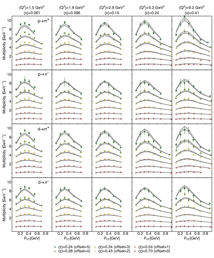
Fig. 3 presents the agreement between the theoretical formula in (3) and the Hermes multiplicities for production of pions off a proton and a deuteron. Different , and bins are displayed as a function of the transverse momentum of the detected hadron . The grey bands are an envelope of the replica of best-fit curves. For every point in we apply a C.L. selection criterion. Points marked with different symbols and colors correspond to different values. There is a strong correlation between and that does not allow us to explore the and dependence of the TMDs separately. Studying the contributions to the /points as a function of the kinematics, we notice that the tends to improve as we move to higher values, where the kinematic approximations of factorization are more reliable. Moreover, usually the increases at lower values.
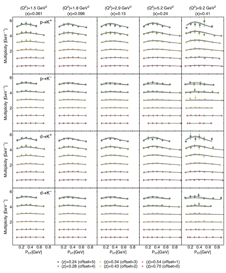
Fig. 4 has same contents and notation as in Fig. 3 but for kaons in the final state. In this case, the trend of the agreement as a function of is not as clear as for the case of pions: good agreement is found also at low .
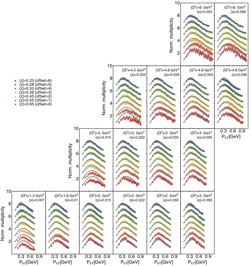
In Fig. 5 we present Compass normalized multiplicities (see Eq. (41)) for production of off a deuteron for different , , and bins as a function of the transverse momentum of the detected hadron . The open marker around the first point in each panel indicates that the first value is fixed and not fitted. The correlation between and is less strong than at Hermes and this allows us to study different bins at fixed . For the highest bins, the agreement is good for all , and . In bins at lower , the descriptions gets worse, especially at low and high . For fixed and high , a good agreement is recovered moving to higher bins (see, e.g., the third line from the top in Fig. 5).
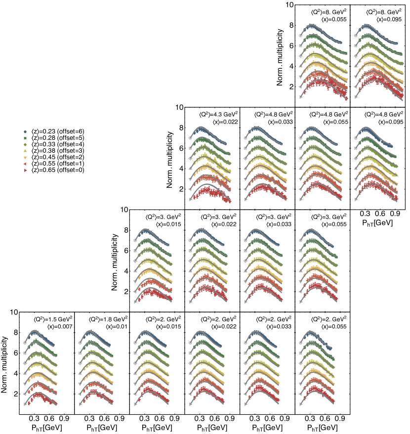
Fig. 6 has same content and notation as in Fig. 5, but for . The same comments on the agreement between theory and the data apply.
Drell–Yan and production
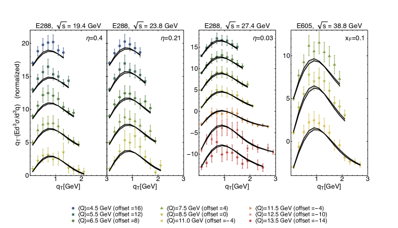
The low energy Drell–Yan data collected by the E288 and E605 experiments at Fermilab have large error bands (see Fig. 7). This is why the values in Tab. 8 are rather low compared to the other data sets.
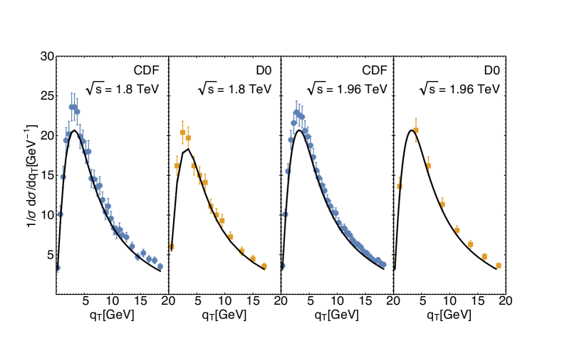
The agreement is also good for boson production, see Tab. 9. The statistics from Run-II is higher, which generates smaller experimental uncertainties and higher , especially for the CDF experiment.
| E288 [200] | E288 [300] | E288 [400] | E605 | |
|---|---|---|---|---|
| Points | 45 | 45 | 78 | 35 |
| points |
| CDF Run I | D0 Run I | CDF Run II | D0 Run II | |
|---|---|---|---|---|
| Points | 31 | 14 | 37 | 8 |
| points |
Fig. 7 displays the cross section for DY events differential with respect to the transverse momentum of the virtual photon, its invariant mass and rapidity . As for the case of SIDIS, the grey bands are the C.L. envelope of the 200 replicas of the fit function. The four panels represents different values for the rapidity or (see Eq. (15)). In each panel, we have plots for different values. The lower is , the less points in we fit (see also Sec. III.2). The hard scale lies in the region GeV. This region is of particular importance, since these “moderate” values should be high enough to safely apply factorization and, at the same time, low enough in order for the nonperturbative effects to not be shaded by transverse momentum resummation.
In Fig. 8 we compare the cross section differential with respect to the transverse momentum of the virtual (namely Eq. (12) integrated over ) with data from CDF and D0 at Tevatron Run I and II. Due to the higher , the range explored in is much larger compared to all the other observables considered. The tails of the distributions deviate from a Gaussian behavior, as it is also evident in the bins at higher in Fig. 7. The band from the replica methodology in this case is much narrower, due to the reduced sensitivity to the intrinsic transverse momenta at and to the limited range of best-fit values for the parameter , which controls soft-gluon emission. As an effect of TMD evolution, the peak shifts from GeV for Drell–Yan events in Fig. 7 to GeV in Fig. 8. The position of the peak is affected both by the perturbative and the nonperturbative part of the Sudakov exponent (see Sec. II.3 and Signori (2016a)). Most of the contributions to the comes from normalization effects and not from the shape in (see Sec. IV.3).
IV.2 Transverse momentum dependence at 1 GeV
The variables and delimit the range in where transverse momentum resummation is computed perturbatively. The parameter enters the nonperturbative Sudakov exponent and quantifies the amount of transverse momentum due to soft gluon radiation that is not included in the perturbative part of the Sudakov form factor. As already explained in Sec. II.3, in this work we fix the value for and in such a way that at GeV the unpolarized TMDs coincide with their nonperturbative input. We leave as a fit parameter.
Tab. 10 summarizes the chosen values of , and the best-fit value for . The latter is given as an average with C.L. uncertainty computed over the set of 200 replicas. We also quote the results obtained from replica 105, since its parameters are very close to the mean values of all replicas. We obtain a value , smaller than the value () obtained in Ref. Konychev and Nadolsky (2006), where however no SIDIS data was taken into consideration, and smaller than the value () chosen in Ref. Echevarria et al. (2014). We stress however that our prescriptions involving both and are different from previous works.
Tab. 11 collects the best-fit values of parameters in the nonperturbative part of the TMDs at GeV (see Eqs. (34) and (35)); as for , we give the average value over the full set of replicas and the standard deviation based on a C.L. (see Sec. III.4), and we also quote the value of replica 105.
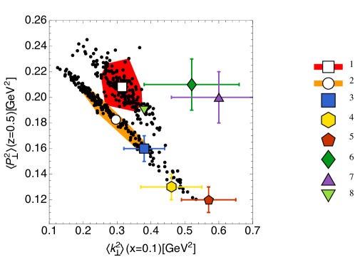
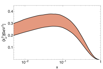
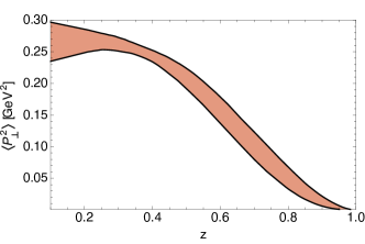
In Fig. 9 we compare different extractions of partonic transverse momenta. The horizontal axis shows the value of the average transverse momentum squared for the incoming parton, (see Eq. (40)). The vertical axis shows the value of , the average transverse momentum squared acquired during the fragmentation process (see Eq. (40)). The white square (label 1) indicates the average values of the two quantities obtained in the present analysis at GeV2. Each black dot around the white square is an outcome of one replica. The red region around the white square contains the of the replicas that are closest to the average value. The same applies to the white circle and the orange region around it (label 2), related to the flavor-independent version of the analysis in Ref. Signori et al. (2013), obtained by fitting only Hermes SIDIS data at an average GeV2 and neglecting QCD evolution. A strong anticorrelation between the transverse momenta is evident in this older analysis. In our new analysis, the inclusion of Drell–Yan and production data adds physical information about TMD PDFs, free from the influence of TMD FFs. This reduces significantly the correlation between and . The confidence region is smaller than in the older analysis. The average values of are similar and compatible within error bands. The values of in the present analysis turn out to be larger than in the older analysis, an effect that is due mainly to Compass data. It must be kept in mind that the two analyses lead also to differences in the and dependence of the transverse momentum squared. This dependence is shown in Fig. 10 (a) for and Fig. 10 (b) for . The bands are computed as the C.L. envelope of the full sets of curves from the 200 replicas. Comparison with other extractions are presented and the legend is detailed in the caption of Fig. 9.
| [GeV-1] | [GeV-1] | [GeV2] | |
|---|---|---|---|
| (fixed) | (fixed) | ||
| All replicas | |||
| Replica 105 |
| TMD PDFs | ||||||
|---|---|---|---|---|---|---|
| [GeV2] | [GeV-2] | |||||
| All replicas | ||||||
| Replica 105 | ||||||
| TMD FFs | ||||||
| [GeV2] | [GeV-2] | [GeV2] | ||||
| All replicas | ||||||
| Replica 105 |
 |
 |
| (a) | (b) |
IV.3 Stability of our results
In this subsection we discuss the effect of modifying some of the choices we made in our default fit. Instead of repeating the fitting procedure with different choices, we limit ourselves to checking how the of a single replica is affected by the modifications.
As starting point we choose replica 105, which, as discussed above, is one of the most representative among the whole replica set. The global d.o.f. of replica 105 is 1.51. We keep all parameters fixed, without performing any new minimization, and we compute the d.o.f. after the modifications described in the following.
First of all, we analyze Hermes data with the same strategy as Compass, i.e., we normalize Hermes data to the value of the first bin in . In this case, the global d.o.f. reduces sharply to 1.27. The partial for the different SIDIS processes measured at Hermes are shown in Table 12. This confirms that normalization effects are the main contribution to the of SIDIS data and have minor effects on TMD-related parameters. In fact, even if we perform a new fit with this modification, the does not improve significantly and parameters do not change much.
| Original | 5.18 | 2.67 | 0.75 | 0.78 | 3.63 | 2.31 | 1.12 | 2.27 |
| Normalized | 1.94 | 1.13 | 0.57 | 0.29 | 1.59 | 0.80 | 0.47 | 0.97 |
We consider the effect of changing the normalization of the -boson data: if we increase the normalization factors quoted in the last row of Tab. 4 by 5%, the quoted in the last row of Tab. 9 drops to 0.66, 0.52, 0.65, 0.68. This effect is also already visible by eye in Fig. 8: the theoretical curves are systematically below the experimental data points, but the shape is reproduced very well.
We consider the sensitivity of our results to the parameterizations adopted for the collinear quark PDFs. The varies from its original value 1.51, obtained with the NLO GJR 2008 parametrization Gluck et al. (2008), to 1.84 using NLO MSTW 2008 Martin et al. (2009), and 1.85 using NLO CJ12 Owens et al. (2013). In both cases, the agreement with Hermes and boson data is not affected significanlty, the agreement with Compass data becomes slightly worse, and the agreement with DY data becomes clearly worse.
An extremely important point is the choice of kinematic cuts. Our default choices are listed in Tabs. 1–4. We consider also more stringent kinematic cuts on SIDIS data: GeV2 and instead of GeV2 and , leaving the other ones unchanged. The number of bins with these cuts reduces from 8059 to 5679 and the decreases to the value 1.23. In addition, if we replace the constraint GeV with GeV, the number of bins reduces to 3380 and the d.o.f. decreases further to 0.96. By adopting the even stricter cut , the number of bins drops to only 477, with a /d.o.f. =1.02. We can conclude that our fit, obtained by fitting data in an extended kinematic region, where TMD factorization may be questioned, works extremely well also in a narrower region, where TMD factorization is expected to be under control.
V Conclusions
In this work we demonstrated for the first time that it is possible to perform a simultaneous fit of unpolarized TMD PDFs and FFs to data of SIDIS, Drell–Yan and boson production at small transverse momentum collected by different experiments. This constitutes the first attempt towards a global fit of and in the context of TMD factorization and with the implementation of TMD evolution at NLL accuracy.
We extracted unpolarized TMDs using 8059 data points with 11 free parameters using a replica methodology. We selected data with GeV2 and . We restricted our fit to the small transverse momentum region, selecting the maximum value of transverse momentum on the basis of phenomenological considerations (see Sec. III). With these choices, we included regions where TMD factorization could be questioned, but we checked that our results describe very well the regions where TMD factorization is supposed to hold. The average /d.o.f. is and can be improved up to 1.02 restricting the kinematic cuts, without changing the parameters (see Sec. IV.3). Most of the discrepancies between experimental data and theory comes from the normalization and not from the transverse momentum shape.
Our fit is performed assuming that the intrinsic transverse momentum dependence of TMD PDFs and FFs can be parametrized by a normalized linear combination of a Gaussian and a weighted Gaussian. We considered that the widths of the Gaussians depend on the longitudinal momenta. We neglected a possible flavor dependence. For the nonperturbative component of TMD evolution, we adopted the choice most often used in the literature (see Sec. II.3).
We plan to release grids of the parametrizations studied in this work via TMDlib Hautmann et al. (2014) to facilitate phenomenological studies for present and future experiments.
In future studies, different functional forms for all the nonperturbative ingredients should be explored, including also a possible flavor dependence of the intrinsic transverse momenta. A more precise analysis from the perturbative point of view is also needed, which should in principle make it possible to relax the tension in the normalization and to describe data at higher transverse momenta. Moreover, the description at low transverse momentum should be properly matched to the collinear fixed-order calculations at high transverse momentum.
Together with an improved theoretical framework, in order to better understand the formalism more experimental data is needed. It would be particularly useful to extend the coverage in , , rapidity, and . The GeV physics program at Jefferson Lab Dudek et al. (2012) will be very important to constrain TMD distributions at large . Additional data from SIDIS (at Compass, at a future Electron-Ion Collider), Drell–Yan (at Compass, at Fermilab), production (at LHC, RHIC, and at A Fixed-Target Experiment at the LHC Brodsky et al. (2013)) will be very important. Measurements related to unpolarized TMD FFs at colliders (at Belle-II, BES-III, at a future International Linear Collider) will be invaluable, since they are presently missing.
Our work focused on quark TMDs. We remark that at present almost nothing is known experimentally about gluon TMDs Mulders and Rodrigues (2001); Echevarria et al. (2015), because they typically require higher-energy scattering processes and they are harder to isolate as compared to quark distributions. Several promising measurements have been proposed in order to extract both the unpolarized and linearly polarized gluon TMDs inside an unpolarized proton. The cleanest possibility would be to look at dijet and heavy quark pair production in electron-proton collisions at a future EIC Boer et al. (2011b); Pisano et al. (2013). Other proposals include isolated photon-pair production at RHIC Qiu et al. (2011) and quarkonium production at the LHC Boer and Pisano (2012); den Dunnen et al. (2014); Signori (2016b); Lansberg et al. (2017).
Testing the formalism of TMD factorization and understanding the structure of unpolarized TMDs is only the first crucial step in the exploration of the 3D proton structure in momentum space and this work opens the way to global determinations of TMDs. Building on this, we can proceed to deepen our understanding of hadron structure via polarized structure function and asymmetries (see, e.g., Refs. Aschenauer et al. (2016); Boglione and Prokudin (2016) and references therein) and, at the same time, to test the impact of hadron structure in precision measurements at high-energies, such as at the LHC. A detailed mapping of hadron structure is essential to interpret data from hadronic collisions, which are among the most powerful tools to look for footprints of new physics.
Acknowledgements.
Discussions with Giuseppe Bozzi are gratefully acknowledged. This work is supported by the European Research Council (ERC) under the European Union’s Horizon 2020 research and innovation program (grant agreement No. 647981, 3DSPIN). AS acknowledges support from U.S. Department of Energy contract DE-AC05-06OR23177, under which Jefferson Science Associates, LLC, manages and operates Jefferson Lab. The work of AS has been funded partly also by the program of the Stichting voor Fundamenteel Onderzoek der Materie (FOM), which is financially supported by the Nederlandse Organisatie voor Wetenschappelijk Onderzoek (NWO).References
- Collins et al. (1989) J. C. Collins, D. E. Soper, and G. F. Sterman, Adv. Ser. Direct. High Energy Phys. 5, 1 (1989), eprint hep-ph/0409313
- Collins (2013) J. Collins, Foundations of perturbative QCD (Cambridge University Press, 2013), ISBN 9781107645257, 9781107645257, 9780521855334, 9781139097826, URL http://www.cambridge.org/de/knowledge/isbn/item5756723
- Angeles-Martinez et al. (2015) R. Angeles-Martinez et al., Acta Phys. Polon. B46, 2501 (2015), eprint 1507.05267
- Rogers (2016) T. C. Rogers, Eur. Phys. J. A52, 153 (2016), eprint 1509.04766
- Bacchetta (2016) A. Bacchetta, Eur. Phys. J. A52, 163 (2016)
- Radici (2016) M. Radici, AIP Conf. Proc. 1735, 020003 (2016)
- Mulders and Tangerman (1996) P. J. Mulders and R. D. Tangerman, Nucl. Phys. B461, 197 (1996), [Erratum: Nucl. Phys.B484,538(1997)], eprint hep-ph/9510301
- Bacchetta et al. (2007) A. Bacchetta, M. Diehl, K. Goeke, A. Metz, P. J. Mulders, and M. Schlegel, JHEP 02, 093 (2007), eprint hep-ph/0611265
- Boer and Mulders (1998) D. Boer and P. J. Mulders, Phys. Rev. D57, 5780 (1998), eprint hep-ph/9711485
- Bacchetta and Mulders (2000) A. Bacchetta and P. J. Mulders, Phys. Rev. D62, 114004 (2000), eprint hep-ph/0007120
- Mulders and Rodrigues (2001) P. J. Mulders and J. Rodrigues, Phys. Rev. D63, 094021 (2001), eprint hep-ph/0009343
- Boer et al. (2016) D. Boer, S. Cotogno, T. van Daal, P. J. Mulders, A. Signori, and Y.-J. Zhou, JHEP 10, 013 (2016), eprint 1607.01654
- Bacchetta and Radici (2011) A. Bacchetta and M. Radici, Phys. Rev. Lett. 107, 212001 (2011), eprint 1107.5755
- Anselmino et al. (2012) M. Anselmino, M. Boglione, and S. Melis, Phys. Rev. D86, 014028 (2012), eprint 1204.1239
- Echevarria et al. (2014) M. G. Echevarria, A. Idilbi, Z.-B. Kang, and I. Vitev, Phys. Rev. D89, 074013 (2014), eprint 1401.5078
- Anselmino et al. (2016) M. Anselmino, M. Boglione, U. D’Alesio, F. Murgia, and A. Prokudin (2016), eprint 1612.06413
- Lu and Schmidt (2010) Z. Lu and I. Schmidt, Phys. Rev. D81, 034023 (2010), eprint 0912.2031
- Barone et al. (2015) V. Barone, M. Boglione, J. O. Gonzalez Hernandez, and S. Melis, Phys. Rev. D91, 074019 (2015), eprint 1502.04214
- Lefky and Prokudin (2015) C. Lefky and A. Prokudin, Phys. Rev. D91, 034010 (2015), eprint 1411.0580
- Anselmino et al. (2013) M. Anselmino, M. Boglione, U. D’Alesio, S. Melis, F. Murgia, and A. Prokudin, Phys. Rev. D87, 094019 (2013), eprint 1303.3822
- Kang et al. (2016) Z.-B. Kang, A. Prokudin, P. Sun, and F. Yuan, Phys. Rev. D93, 014009 (2016), eprint 1505.05589
- Signori (2016a) A. Signori, Ph.D. thesis, Vrije U., Amsterdam (2016a), URL http://inspirehep.net/record/1493030/files/Thesis-2016-Signori.pdf
- Signori et al. (2013) A. Signori, A. Bacchetta, M. Radici, and G. Schnell, JHEP 11, 194 (2013), eprint 1309.3507
- Bacchetta et al. (2015) A. Bacchetta, M. G. Echevarria, P. J. G. Mulders, M. Radici, and A. Signori, JHEP 11, 076 (2015), eprint 1508.00402
- Collins et al. (2016) J. Collins, L. Gamberg, A. Prokudin, T. C. Rogers, N. Sato, and B. Wang, Phys. Rev. D94, 034014 (2016), eprint 1605.00671
- Boer et al. (2011a) D. Boer et al. (2011a), eprint 1108.1713
- Bacchetta et al. (2008a) A. Bacchetta, D. Boer, M. Diehl, and P. J. Mulders, JHEP 08, 023 (2008a), eprint 0803.0227
- Chekanov et al. (2009) S. Chekanov et al. (ZEUS), Phys. Lett. B682, 8 (2009), eprint 0904.1092
- Andreev et al. (2014) V. Andreev et al. (H1), Eur. Phys. J. C74, 2814 (2014), eprint 1312.4821
- Collins and Soper (1981) J. C. Collins and D. E. Soper, Nucl. Phys. B193, 381 (1981), [Erratum: Nucl. Phys.B213,545(1983)]
- Collins et al. (1985) J. C. Collins, D. E. Soper, and G. F. Sterman, Nucl. Phys. B250, 199 (1985)
- Ji and Yuan (2002) X.-d. Ji and F. Yuan, Phys. Lett. B543, 66 (2002), eprint hep-ph/0206057
- Ji et al. (2005) X.-d. Ji, J.-p. Ma, and F. Yuan, Phys. Rev. D71, 034005 (2005), eprint hep-ph/0404183
- Aybat and Rogers (2011) S. M. Aybat and T. C. Rogers, Phys. Rev. D83, 114042 (2011), eprint 1101.5057
- Echevarria et al. (2012) M. G. Echevarria, A. Idilbi, and I. Scimemi, JHEP 07, 002 (2012), eprint 1111.4996
- Echevarria et al. (2013) M. G. Echevarria, A. Idilbi, A. Schäfer, and I. Scimemi, Eur. Phys. J. C73, 2636 (2013), eprint 1208.1281
- Collins and Rogers (2013) J. C. Collins and T. C. Rogers, Phys. Rev. D87, 034018 (2013), eprint 1210.2100
- Matevosyan et al. (2012) H. H. Matevosyan, W. Bentz, I. C. Cloet, and A. W. Thomas, Phys. Rev. D85, 014021 (2012), eprint 1111.1740
- Boglione et al. (2017) M. Boglione, J. Collins, L. Gamberg, J. O. Gonzalez-Hernandez, T. C. Rogers, and N. Sato, Phys. Lett. B766, 245 (2017), eprint 1611.10329
- Moffat et al. (2017) E. Moffat, W. Melnitchouk, T. C. Rogers, and N. Sato (2017), eprint 1702.03955
- Echevarria et al. (2016) M. G. Echevarria, I. Scimemi, and A. Vladimirov, JHEP 09, 004 (2016), eprint 1604.07869
- Boer and Vogelsang (2006) D. Boer and W. Vogelsang, Phys. Rev. D74, 014004 (2006), eprint hep-ph/0604177
- Arnold et al. (2009) S. Arnold, A. Metz, and M. Schlegel, Phys. Rev. D79, 034005 (2009), eprint 0809.2262
- Patrignani et al. (2016) C. Patrignani et al. (Particle Data Group), Chin. Phys. C40, 100001 (2016)
- Lambertsen and Vogelsang (2016) M. Lambertsen and W. Vogelsang, Phys. Rev. D93, 114013 (2016), eprint 1605.02625
- Parisi and Petronzio (1979) G. Parisi and R. Petronzio, Nucl. Phys. B154, 427 (1979)
- Altarelli et al. (1984) G. Altarelli, R. K. Ellis, M. Greco, and G. Martinelli, Nucl. Phys. B246, 12 (1984)
- Bozzi et al. (2011) G. Bozzi, S. Catani, G. Ferrera, D. de Florian, and M. Grazzini, Phys. Lett. B696, 207 (2011), eprint 1007.2351
- Boer and den Dunnen (2014) D. Boer and W. J. den Dunnen, Nucl. Phys. B886, 421 (2014), eprint 1404.6753
- Laenen et al. (2000) E. Laenen, G. F. Sterman, and W. Vogelsang, Phys. Rev. Lett. 84, 4296 (2000), eprint hep-ph/0002078
- Qiu and Zhang (2001) J.-w. Qiu and X.-f. Zhang, Phys. Rev. D63, 114011 (2001), eprint hep-ph/0012348
- Davies and Stirling (1984) C. T. H. Davies and W. J. Stirling, Nucl. Phys. B244, 337 (1984)
- Frixione et al. (1999) S. Frixione, P. Nason, and G. Ridolfi, Nucl. Phys. B542, 311 (1999), eprint hep-ph/9809367
- Bozzi et al. (2006) G. Bozzi, S. Catani, D. de Florian, and M. Grazzini, Nucl. Phys. B737, 73 (2006), eprint hep-ph/0508068
- Nadolsky et al. (2000) P. M. Nadolsky, D. R. Stump, and C. P. Yuan, Phys. Rev. D61, 014003 (2000), [Erratum: Phys. Rev.D64,059903(2001)], eprint hep-ph/9906280
- Landry et al. (2003) F. Landry, R. Brock, P. M. Nadolsky, and C. P. Yuan, Phys. Rev. D67, 073016 (2003), eprint hep-ph/0212159
- Konychev and Nadolsky (2006) A. V. Konychev and P. M. Nadolsky, Phys. Lett. B633, 710 (2006), eprint hep-ph/0506225
- Aidala et al. (2014) C. A. Aidala, B. Field, L. P. Gamberg, and T. C. Rogers, Phys. Rev. D89, 094002 (2014), eprint 1401.2654
- Collins and Rogers (2015) J. Collins and T. Rogers, Phys. Rev. D91, 074020 (2015), eprint 1412.3820
- Scimemi and Vladimirov (2017) I. Scimemi and A. Vladimirov, JHEP 03, 002 (2017), eprint 1609.06047
- D’Alesio et al. (2014a) U. D’Alesio, M. G. Echevarria, S. Melis, and I. Scimemi, JHEP 11, 098 (2014a), eprint 1407.3311
- Gluck et al. (2008) M. Gluck, P. Jimenez-Delgado, and E. Reya, Eur. Phys. J. C53, 355 (2008), eprint 0709.0614
- Buckley et al. (2015) A. Buckley, J. Ferrando, S. Lloyd, K. Nordström, B. Page, M. Rüfenacht, M. Schönherr, and G. Watt, Eur. Phys. J. C75, 132 (2015), eprint 1412.7420
- de Florian et al. (2015) D. de Florian, R. Sassot, M. Epele, R. J. Hernández-Pinto, and M. Stratmann, Phys. Rev. D91, 014035 (2015), eprint 1410.6027
- de Florian et al. (2007) D. de Florian, R. Sassot, and M. Stratmann, Phys. Rev. D75, 114010 (2007), eprint hep-ph/0703242
- de Florian et al. (2017) D. de Florian, M. Epele, R. J. Hernandez-Pinto, R. Sassot, and M. Stratmann (2017), eprint 1702.06353
- Bacchetta et al. (2008b) A. Bacchetta, L. P. Gamberg, G. R. Goldstein, and A. Mukherjee, Phys. Lett. B659, 234 (2008b), eprint 0707.3372
- Pasquini et al. (2008) B. Pasquini, S. Cazzaniga, and S. Boffi, Phys. Rev. D78, 034025 (2008), eprint 0806.2298
- Avakian et al. (2010) H. Avakian, A. V. Efremov, P. Schweitzer, and F. Yuan, Phys. Rev. D81, 074035 (2010), eprint 1001.5467
- Bacchetta et al. (2010) A. Bacchetta, M. Radici, F. Conti, and M. Guagnelli, Eur. Phys. J. A45, 373 (2010), eprint 1003.1328
- Burkardt and Pasquini (2016) M. Burkardt and B. Pasquini, Eur. Phys. J. A52, 161 (2016), eprint 1510.02567
- Bacchetta et al. (2002) A. Bacchetta, R. Kundu, A. Metz, and P. J. Mulders, Phys. Rev. D65, 094021 (2002), eprint hep-ph/0201091
- Schweitzer et al. (2013) P. Schweitzer, M. Strikman, and C. Weiss, JHEP 01, 163 (2013), eprint 1210.1267
- Airapetian et al. (2013) A. Airapetian et al. (HERMES), Phys. Rev. D87, 074029 (2013), eprint 1212.5407
- Adolph et al. (2013) C. Adolph et al. (COMPASS), Eur. Phys. J. C73, 2531 (2013), [Erratum: Eur. Phys. J.C75,no.2,94(2015)], eprint 1305.7317
- Anselmino et al. (2014) M. Anselmino, M. Boglione, J. O. Gonzalez Hernandez, S. Melis, and A. Prokudin, JHEP 04, 005 (2014), eprint 1312.6261
- Landry et al. (2001) F. Landry, R. Brock, G. Ladinsky, and C. P. Yuan, Phys. Rev. D63, 013004 (2001), eprint hep-ph/9905391
- D’Alesio et al. (2014b) U. D’Alesio, M. G. Echevarria, S. Melis, and I. Scimemi, JHEP 11, 098 (2014b), eprint 1407.3311
- Ito et al. (1981) A. S. Ito et al., Phys. Rev. D23, 604 (1981)
- Moreno et al. (1991) G. Moreno et al., Phys. Rev. D43, 2815 (1991)
- Affolder et al. (2000) T. Affolder et al. (CDF), Phys. Rev. Lett. 84, 845 (2000), eprint hep-ex/0001021
- Abbott et al. (2000) B. Abbott et al. (D0), Phys. Rev. D61, 032004 (2000), eprint hep-ex/9907009
- Aaltonen et al. (2012) T. Aaltonen et al. (CDF), Phys. Rev. D86, 052010 (2012), eprint 1207.7138
- Abazov et al. (2008) V. M. Abazov et al. (D0), Phys. Rev. Lett. 100, 102002 (2008), eprint 0712.0803
- Abulencia et al. (2007) A. Abulencia et al. (CDF), J. Phys. G34, 2457 (2007), eprint hep-ex/0508029
- Catani et al. (2009) S. Catani, L. Cieri, G. Ferrera, D. de Florian, and M. Grazzini, Phys. Rev. Lett. 103, 082001 (2009), eprint 0903.2120
- Bacchetta et al. (2013) A. Bacchetta, A. Courtoy, and M. Radici, JHEP 03, 119 (2013), eprint 1212.3568
- Radici et al. (2015) M. Radici, A. Courtoy, A. Bacchetta, and M. Guagnelli, JHEP 05, 123 (2015), eprint 1503.03495
- Forte et al. (2002) S. Forte, L. Garrido, J. I. Latorre, and A. Piccione, JHEP 05, 062 (2002), eprint hep-ph/0204232
- Ball et al. (2009) R. D. Ball, L. Del Debbio, S. Forte, A. Guffanti, J. I. Latorre, A. Piccione, J. Rojo, and M. Ubiali (NNPDF), Nucl. Phys. B809, 1 (2009), [Erratum: Nucl. Phys.B816,293(2009)], eprint 0808.1231
- Ball et al. (2010) R. D. Ball, L. Del Debbio, S. Forte, A. Guffanti, J. I. Latorre, J. Rojo, and M. Ubiali, Nucl. Phys. B838, 136 (2010), eprint 1002.4407
- Epele et al. (2012) M. Epele, R. Llubaroff, R. Sassot, and M. Stratmann, Phys. Rev. D86, 074028 (2012), eprint 1209.3240
- James and Roos (1975) F. James and M. Roos, Comput. Phys. Commun. 10, 343 (1975)
- Aid et al. (1995) S. Aid et al. (H1), Phys. Lett. B356, 118 (1995), eprint hep-ex/9506012
- Ladinsky and Yuan (1994) G. A. Ladinsky and C. P. Yuan, Phys. Rev. D50, R4239 (1994), eprint hep-ph/9311341
- Sun et al. (2014) P. Sun, J. Isaacson, C. P. Yuan, and F. Yuan (2014), eprint 1406.3073
- Schweitzer et al. (2010) P. Schweitzer, T. Teckentrup, and A. Metz, Phys. Rev. D81, 094019 (2010), eprint 1003.2190
- Martin et al. (2009) A. D. Martin, W. J. Stirling, R. S. Thorne, and G. Watt, Eur. Phys. J. C63, 189 (2009), eprint 0901.0002
- Owens et al. (2013) J. F. Owens, A. Accardi, and W. Melnitchouk, Phys. Rev. D87, 094012 (2013), eprint 1212.1702
- Hautmann et al. (2014) F. Hautmann, H. Jung, M. Krämer, P. J. Mulders, E. R. Nocera, T. C. Rogers, and A. Signori, Eur. Phys. J. C74, 3220 (2014), eprint 1408.3015
- Dudek et al. (2012) J. Dudek et al., Eur. Phys. J. A48, 187 (2012), eprint 1208.1244
- Brodsky et al. (2013) S. J. Brodsky, F. Fleuret, C. Hadjidakis, and J. P. Lansberg, Phys. Rept. 522, 239 (2013), eprint 1202.6585
- Echevarria et al. (2015) M. G. Echevarria, T. Kasemets, P. J. Mulders, and C. Pisano, JHEP 07, 158 (2015), eprint 1502.05354
- Boer et al. (2011b) D. Boer, S. J. Brodsky, P. J. Mulders, and C. Pisano, Phys. Rev. Lett. 106, 132001 (2011b), eprint 1011.4225
- Pisano et al. (2013) C. Pisano, D. Boer, S. J. Brodsky, M. G. A. Buffing, and P. J. Mulders, JHEP 10, 024 (2013), eprint 1307.3417
- Qiu et al. (2011) J.-W. Qiu, M. Schlegel, and W. Vogelsang, Phys. Rev. Lett. 107, 062001 (2011), eprint 1103.3861
- Boer and Pisano (2012) D. Boer and C. Pisano, Phys. Rev. D86, 094007 (2012), eprint 1208.3642
- den Dunnen et al. (2014) W. J. den Dunnen, J. P. Lansberg, C. Pisano, and M. Schlegel, Phys. Rev. Lett. 112, 212001 (2014), eprint 1401.7611
- Signori (2016b) A. Signori, Few Body Syst. 57, 651 (2016b), eprint 1602.03405
- Lansberg et al. (2017) J.-P. Lansberg, C. Pisano, and M. Schlegel (2017), eprint 1702.00305
- Aschenauer et al. (2016) E. C. Aschenauer, U. D’Alesio, and F. Murgia, Eur. Phys. J. A52, 156 (2016), eprint 1512.05379
- Boglione and Prokudin (2016) M. Boglione and A. Prokudin, Eur. Phys. J. A52, 154 (2016), eprint 1511.06924