High-resolution imaging spectroscopy of two micro-pores
and an arch filament system in a small emerging-flux region

Abstract

Context. Emerging flux regions mark the first stage in the accumulation of magnetic flux eventually leading to pores, sunspots, and (complex) active regions. These flux regions are highly dynamic, show a variety of fine structure, and in many cases live only for a short time (less than a day) before dissolving quickly into the ubiquitous quiet-Sun magnetic field.

Aims. The purpose of this investigation is to characterize the temporal evolution of a minute emerging flux region, the associated photospheric and chromospheric flow fields, and the properties of the accompanying arch filament system. We aim to explore flux emergence and decay processes and investigate if they scale with structure size and magnetic flux contents.

Methods. This study is based on imaging spectroscopy with the Göttingen Fabry-Pérot Interferometer at the Vacuum Tower Telescope, Observatorio del Teide, Tenerife, Spain on 2008 August 7. Photospheric horizontal proper motions were measured with Local Correlation Tracking using broadband images restored with multi-object multi-frame blind deconvolution. Cloud model (CM) inversions of line scans in the strong chromospheric absorption H$\alpha$ $\lambda 656.28$ nm line yielded CM parameters (Doppler velocity, Doppler width, optical thickness, and source function), which describe the cool plasma contained in the arch filament system.

Results. The high-resolution observations cover the decay and convergence of two micro-pores with diameters of less than one arcsecond and provide decay rates for intensity and area. The photospheric horizontal flow speed is suppressed near the two micro-pores indicating that the magnetic field is already sufficiently strong to affect the convective energy transport. The micro-pores are accompanied by a small arch filament system as seen in H$\alpha$, where small-scale loops connect two regions with H$\alpha$ line-core brightenings containing an emerging flux region with opposite polarities. The Doppler width, optical thickness, and source function reach the largest values near the H$\alpha$ line-core brightenings. The chromospheric velocity of the cloud material is predominantly directed downwards near the footpoints of the loops with velocities of up to 12 km s^-1, whereas loop tops show upward motions of about 3 km s^-1. Some of the loops exhibit signs of twisting motions along the loop axis.

Conclusions. Micro-pores are the smallest magnetic field concentrations leaving a photometric signature in the photosphere. In the observed case, they are accompanied by a miniature arch filament system indicative of newly emerging flux in the form of $\Omega$-loops. Flux emergence and decay take place on a time-scale of about two days, whereas the photometric decay of the micro-pores is much more rapid (a few hours), which is consistent with the incipient submergence of $\Omega$-loops. Considering lifetime and evolution timescales, impact on the surrounding photospheric proper motions, and flow speed of the chromospheric plasma at the loop tops and footpoints, the results are representative for the smallest emerging flux regions still recognizable as such.

1 Introduction

Solar activity is intimately linked to the presence of magnetic fields on the solar surface. Small-scale magnetic fields emerge within the interior of supergranular cells, and they are transported by a radial flow pattern to the boundaries of the cells (Martin, 1988). The stronger magnetic fields appear in a multi-stage process eventually leading to pores, sunspots, and (complex) active regions (Zwaan, 1985; Rezaei et al., 2012). The first indications of newly emerging flux are ephemeral regions with dimensions of about 30 Mm and a total magnetic flux of up to $10^{20}$ Mx. These small-scale, bipolar magnetic flux concentrations spring up everywhere on the solar surface. They continuously replenish the quiet-Sun magnetic field, completely renewingit about every 14 hours (Hagenaar, 2001; Guglielmino et al., 2012). Emerging $\Omega$-loops at granular scale were reported by Martínez González et al. (2010). When such loops rise trough the photosphere their mean velocity can reach up to 3 km s^-1. Once the loops reach the upper photosphere, their magnetic field is almost vertical at the footpoints. In the chromosphere, the mean upflow velocity climbs to 12 km s^-1, and the energy contained in the loops system is at least $1.4\times 10^{6}$ – $2.2\times 10^{7}$ erg cm^-2 s^-1 in the lower chromosphere (Martínez González et al., 2010). The emerging fields are transported by supergranular flows migrating toward the network (Orozco Suárez et al., 2012).

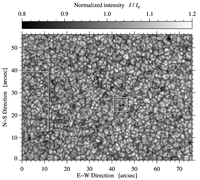
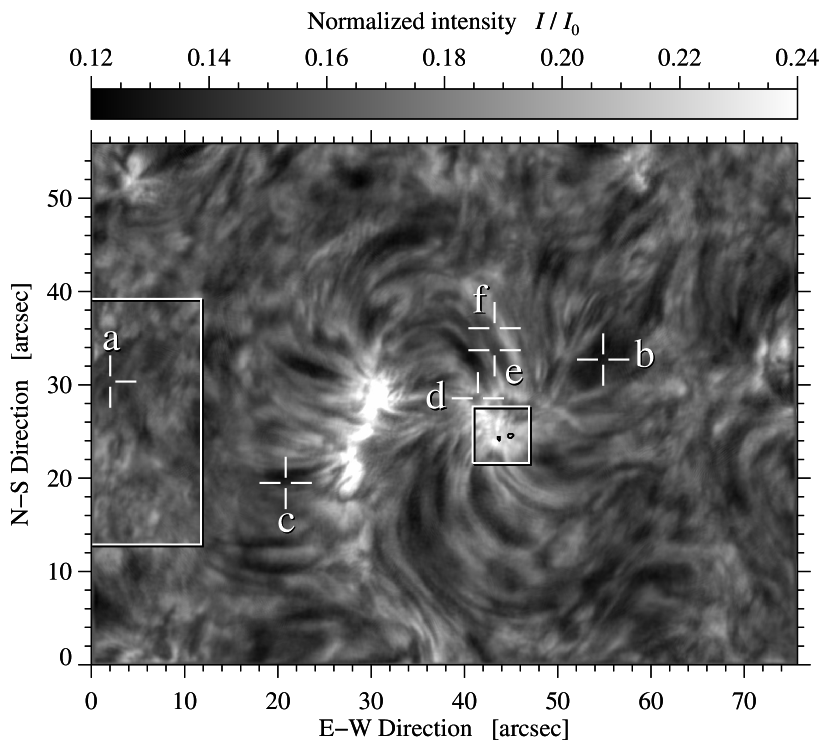
Figure 1: MOMFBD-restored broadband image (top) at about $\lambda$600 nm of micro-pores (white square in the center in both images) in an EFR observed with the GFPI at 08:07 UT on 2008 August 7. H$\alpha$ line-core intensity image corresponding to the broadband image (bottom). The white rectangle on the left outlines the region used for computing the average H$\alpha$ quiet-Sun spectral profile. Crosses ‘✛’ and alphabetic labels mark the locations of six contrast profiles plotted in Fig. 5. The black contours indicate the position of the micro-pores.

The initial expansion rate of the bipoles is about 2 km s^-1 (Harvey & Martin, 1973). Once the magnetic field becomes sufficiently strong (i.e., the filling factor becomes sufficiently high), ‘micro-pores’ appear as a photospheric signatures of flux emergence (Scharmer et al., 2002; Rouppe van der Voort et al., 2005). They change their appearance between elongated features, which are darker in the center and have their maximum brightness at the edges (ribbons), and more circular magnetic structures (flowers), adapting the nomenclature of Rouppe van der Voort et al. (2005). The definitions were made based on G-band data. Micro-pores are at the very low end of the statistical size distribution of pores (Verma & Denker, 2014). Once pores are present, sunspots are eventually formed by coalescence of newly emerged flux (Schlichenmaier et al., 2010; Rezaei et al., 2012).

The dynamics of emerging flux regions (EFRs) are characterized by a transient state (Zwaan, 1985) of magnetic field lines rising within granular convection. On timescales of about 10 minutes (photospheric crossing time), emerging field lines form a pattern of aligned dark intergranular lanes (Strous et al., 1996). When reaching chromospheric heights, the magnetic loops become visible in H$\alpha$, and material gradually drains from the loops. This and convective collapse (Cheung et al., 2008) at the footpoints of the loops lead to strong downflows.

Arch filament systems (AFS) connecting the two opposite magnetic polarities of newly emerging flux are prominently visible in line-core filtergrams of the strong chromospheric absorption line H$\alpha$ and also, but less pronounced, in the Ca ii H & K lines (Bruzek, 1969). Downflows in the range of 30 – 50 km s^-1 occur near both footpoints of dark filaments, whereas loop tops rise with about 1.5 – 20 km s^-1 (Bruzek, 1969; Zwaan, 1985; Chou & Zirin, 1988; Lites et al., 1998). The arched filaments are typically confined below 10 Mm. Bruzek (1969) relates the length of the filaments (20 – 30 Mm) to the size of supergranular network cells. The height of the arches is typically 5 – 15 Mm, and the width of individual filaments is just a few megameters with a lifetime of about 30 minutes (Bruzek, 1967). However, individual loops of the AFS can reach heights of up to 25 Mm and a mean length of about 20 – 40 Mm (Tsiropoula et al., 1992). In general, the appearance of an AFS remains the same for several hours, whereas significant changes occur only along with the growth of the sunspot group, that is after about three days the AFS vanishes.

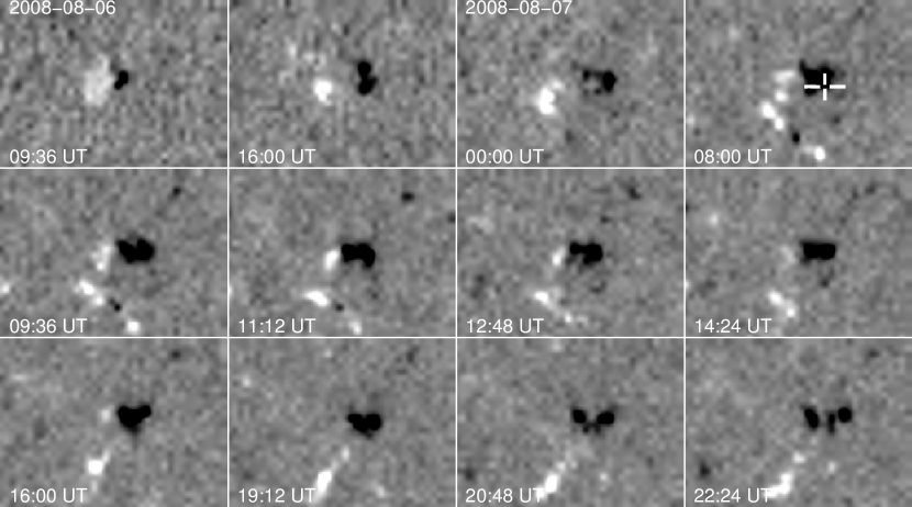
Figure 2: SoHO/MDI time series of a small EFR on 2008 August 6 and 7. Each panel has the same size as the high-resolution image in Fig. 1. The magnetograms were scaled between $\pm$100 G and resampled to a four times finer grid for better display. The cross ✛’ indicate the position of the micro-pores in Fig. 1 using the magnetogram closest in time.

AFS are mainly observed in H$\alpha$, and one method to analyze H$\alpha$ spectra is cloud modeling. The cloud model (CM) assumes that absorbing chromospheric plasma is suspended by the magnetic field above the photosphere (Beckers, 1964). A broad spectrum of solar fine structure was investigated using CM inversions, for example, H$\alpha$ upflow events (Lee et al., 2000), dark mottles in the chromospheric network (Lee et al., 2000; Al et al., 2004; Contarino et al., 2009; Bostanci, 2011), superpenumbral fibrils (Alissandrakis et al., 1990), AFSs (Alissandrakis et al., 1990; Contarino et al., 2009), and filaments (Schmieder et al., 1991). Such inversions are attractive mainly because of the inherent simplicity of the model and the scarcity of other well established inversion schemes for strong chromospheric absorption lines such as H$\alpha$ (cf., Molowny-Horas et al., 1999; Tziotziou et al., 2001). However, refinements of CM inversions have been implemented including the differential cloud model (Mein & Mein, 1988), the addition of a variable source function and velocity gradients (Mein et al., 1996; Heinzel et al., 1999), the embedded cloud model (Chae, 2014), and the two-cloud model (Hong et al., 2014). Bostanci & Erdogan (2010) examined the impact of observed and theoretical quiet-Sun background profiles on CM inversions and concluded that synthetic H$\alpha$ profiles based on non-local thermodynamic equilibrium (NLTE) calculations perform better than profiles derived directly from the data.

Physical processes including radiation, convection, conduction, and magnetic field generation and decay play an important and prominent role in the solar atmosphere. To fully appreciate the dynamics of solar fine structure, simultaneous multi-wavelengths observations at different layers of the Sun are crucial. Wedemeyer-Böhm et al. (2009) critically reviewed the links between the photosphere, chromosphere, and corona of the Sun. They affirm that these atmospheric layers are coupled by the magnetic field at many different spatial scales. Thus loops, as the ones found in AFS, reach from the photosphere to the chromosphere and corona, where they encounter physical conditions differing by orders of magnitude in temperature and gas density. The present study strives to contribute to the quantitative description of EFRs and AFSs. Some of the key questions related to this study are the following: Do morphological evolution and statistical properties of micro-pores imply a specific flux emergence scenario or flux dispersion mechanism (Sect. 4.1)? Which physical quantities are most suitable to restrain theoretical models? Can the results of CM inversions help to identify distinct chromospheric features (cluster analysis in Sect. 3)?

In Sect. 2, we briefly introduce the observations, image processing, and image restoration techniques. The data analysis is described in Sect. 3. Sect. 4 puts forward the results, where we first examine the two micro-pores, then determine the photospheric horizontal proper motions associated with the EFR, and finally scrutinize the chromospheric response of emerging flux, which includes Doppler velocities, CM inversions, and parameters characterizing the AFS. We conclude our study by comparing our results with the most recent findings and synoptic literature concerning EFRs and AFSs (Sect. 5). Initial results were presented in Denker & Tritschler (2009).

2 Observations

A small EFR at heliographic coordinates E28.5^∘ and S7.91^∘ ($\mu=\cos\theta=0.86$) was observed on 2008 August 7 with the Vacuum Tower Telescope (VTT, von der Lühe, 1998) at Observatorio del Teide, Tenerife, Spain. Imaging spectroscopy in the strong chromospheric absorption line H$\alpha$ $\lambda 656.28$ nm was carried out with the Göttingen Fabry-Pérot Interferometer (GFPI, Puschmann et al., 2006; Bello González & Kneer, 2008). The field-of-view (FOV) of the instrument is $77.1\arcsec\times 58.2\arcsec$ ($688\times 520$ pixels after 2$\times$2-pixel binning) with an image scale of 0.112″ pixel^-1. All data were taken under good seeing conditions (Fried-parameter $r_{0}>15$ cm for most of the time) with real-time image correction provided by the Kiepenheuer Adaptive Optics System (KAOS, von der Lühe et al., 2003; Berkefeld et al., 2010).

Four short time series of simultaneous broad- and narrow-band images were acquired with the GFPI during the time period from 07:54 – 08:37 UT (see Fig. 1). The observations were paused twice for about six minutes to take flat-field images at solar disk center and continuum images with an artificial light source. The AO system experienced a few interruptions while tracking on solar granulation. From the 54 time series, 17 data sets (08:07 – 08:16 UT) have been selected for a more detailed analysis because of very good seeing conditions and continuous AO correction. Post-processing with Multi-Object Multi-Frame Blind Deconvolution (MOMFBD, Löfdahl, 2002; van Noort et al., 2005) as described in Sect. 4.4 of de la Cruz Rodríguez et al. (2015) further improves the spatial resolution and contrast of the imaging spectroscopic data.

Each spectral scan of narrow-band images covers 61 equidistant ($\delta\lambda=3.13$ pm) positions in the strong chromospheric absorption line H$\alpha$ $\lambda$656.28 nm, i.e., a spectral window of $\Delta\lambda=0.189$ nm centered on the line core. Eight images were taken at each position to increase the signal-to-noise ratio in preparation for MOMFBD. With an exposure time of 15 ms, the cadence of a spectral scan with $61\times 8=488$ single exposures is $\Delta t=34$ s. Thus, the total duration of the selected time series is $\Delta T\approx 10$ min. In some instances, scans of the other time series are used, for example, when determining the lifetimes of micro-pores.

Finally, we matched our high-resolution observations to 96-minute cadence, full-disk magnetograms of the Solar and Heliospheric Observatory/Michelson Doppler Imager (SoHO/MDI Scherrer et al., 1995). The magnetograms have $1024\times 1024$ pixels and an image scale of 1.986″ pixel^-1. Thus, the image scales of the GFPI and MDI data roughly differ by a factor of twenty, that is, a magnetogram section of just $39\times 29$ pixels corresponds to the GFPI FOV. The magnetograms selected for the time series depicted in Fig. 2 were chosen taking into account some data gaps and the noise being present in the magnetograms. The cadence of the first row is about four hours and about 96 minutes in the other two rows.

3 Data analysis

3.1 Local correlation tracking

Horizontal proper motions are derived from the time series of 17 broadband images using local correlation tracking (LCT, November & Simon, 1988) as described in Verma & Denker (2011). However, the data have not been corrected for geometrical foreshortening because of the small FOV and its proximity to disk center. The input parameters selected for LCT are a cadence of $\Delta t=34$ s, an averaging time of $\Delta T\approx 10$ min, and a Gaussian sampling window with a $\mathrm{FWHM}=600$ km (the Gaussian used as a high-pass filter has a full-width-at-half-maximum $\mathrm{FWHM}=1200$ km). The image scale of the GFPI broadband and Hinode/BFI G-band (Kosugi et al., 2007; Tsuneta et al., 2008) images are almost the same, thus facilitating a straightforward comparison of flow fields derived from these two instruments.

3.2 Cloud model inversions

Some characteristics of strong chromospheric absorption lines are easier to discover in intensity contrast profiles, which are given as

$$C(\lambda)=\frac{I(\lambda)-I_{0}(\lambda)}{I_{0}(\lambda)}\,,$$ (1)

where $I(\lambda)$ and $I_{0}(\lambda)$ denote the observed and the average quiet-Sun spectral profiles, respectively. Beckers (1964) assumes in his model a cloud of absorbing material suspended by the magnetic field above the photosphere, and he provides a relationship between the intensity contrast profile $C(\lambda)$ and four free fit parameters describing the cloud material, that is, the central wavelength of the absorption profile $\lambda_{c}$, the Doppler width of the absorption profile $\Delta\lambda_{D}$, the optical thickness $\tau_{0}$ of the cloud at the central wavelength, and the source function $S$:

$$C(\lambda) = \left[\frac{S}{I_{0}(\lambda)}-1\right]\Big{(}1-\exp\big{[}-\tau(\lambda)\big{]}\Big{)}\quad{\rm with}$$ (2)

$$\tau(\lambda) = \tau_{0}\exp\left[-\left(\frac{\lambda-\lambda_{c}}{\Delta\lambda_{D}}\right)^{2}\right]$$ (3)

The line-of-sight (LOS) velocity $v_{\mathrm{LOS}}$ of the cloud can be derived, once $\lambda_{c}$ is known, according to

$$v_{\mathrm{LOS}}=c\,\frac{\lambda_{c}-\lambda_{0}}{\lambda_{0}}\,,$$ (4)

where $\lambda_{0}$ is the central wavelength of the strong chromospheric absorption line averaged over a quiet-Sun area and $c$ the speed of light.

The quiet-Sun profile $I_{0}(\lambda)$ is computed within an about 10″-wide region to the East of the EFR (see white rectangle in Fig. 1). The selection of $I_{0}(\lambda)$ has a strong impact on the results of the CM analysis (Tziotziou et al., 2003), for example, lateral radiative exchange affects the conditions of the cloud material. The selected quiet-Sun region is at the periphery of AFS, it does not show any features with strong absorption in H$\alpha$, and chromospheric velocities are low. Therefore, this quiet-Sun region is the best choice within the available FOV. We carried out some tests using different samples within this region to create different quiet-Sun profiles. The results from CM inversions were basically identical, which is not the case for other ‘quiet’ settings within the FOV, which contained either absorption features or exhibited high chromospheric velocities. Line shifts are corrected by linear interpolation before averaging the profiles. Assuming that up- and downflows in the quiet Sun are balanced and that the convective blueshift of spectral lines is negligible in the chromosphere, the mean velocity is set to zero and used as a reference for the entire FOV. In this study, the quiet-Sun profile $I_{0}(\lambda)$ is computed from the data itself. However, Bostanci (2011) demonstrated that theoretical profiles from NLTE calculations may compare favorably to profiles derived directly from observations.

Figure 3: Map of the $\chi^{2}$ goodness-of-fit statistics, where bright regions indicate significant differences between the observed and fitted profiles, in particular near the footpoints of the AFS.

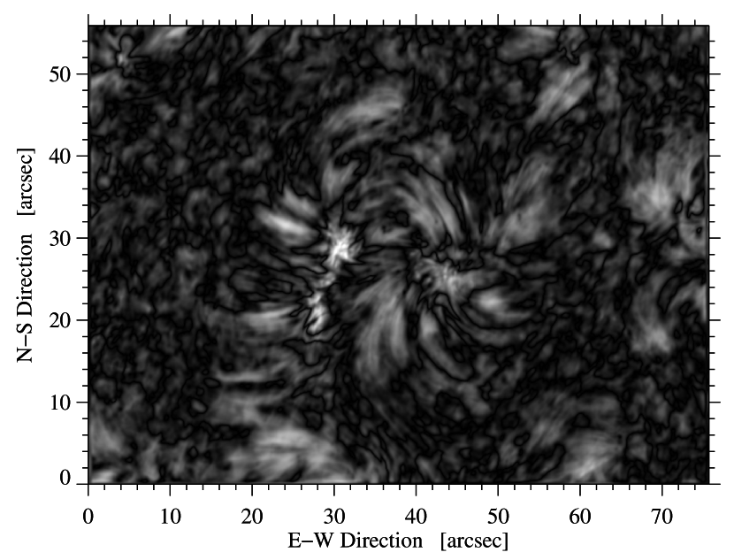
Figure 4: Map of the absolute contrast for each spectral profile. The highest (positive) contrasts correspond to the bright regions in the H$\alpha$ line-core intensity image shown in Fig. 1.

Two steps are required in the CM inversions to efficiently analyze the millions of spectral profiles obtained with imaging spectroscopy: (1) Contrast profiles are computed for 50 000 random CM input parameters, which are restricted to the intervals $\tau_{0}\in[0,3]$, $v_{\mathrm{LOS}}\in[-90,+90]$ km s^-1, $\Delta\lambda_{D}\in[0,70]$ pm, and $S\in[0,0.4]$, where the source function $S$ is given in quiet-Sun intensity units. In addition, the histograms of the parameters have to closely match those of the observations. This requires some a priori knowledge acquired by dropping the last assumption for a representative sample of contrast profiles. Each observed profile is then compared against the 50 000 templates, and the CM parameters of the closest match (smallest $\chi^{2}$-values) are saved. (2) The saved CM parameters are the initial estimates to perform a Levenberg-Markwardt least-squares minimization (Moré, 1977; Moré & Wright, 1993) using the MPFIT software package (Markwardt, 2009). The quiet-Sun spectral profile is handed to the fitting routine as private data avoiding common block variables, and MPFIT’s diagnostic capabilities provide the means to easily discriminate between successful fits and situations, where the iterative algorithm does not converge.

Mediocre fits result in high $\chi^{2}$-values (Fig. 3), which are cospatial with the H$\alpha$ line-core brightenings at the footpoints of the dark filamentary features of the AFS. In addition, for much of the area covered with granulation, the $\chi^{2}$ goodness-of-fit statistics is low. Good CM inversions correspond in general to regions, where the contrast profiles exhibit enhanced contrast as is evident in Fig. 4 for the AFS. Only for regions with high positive contrasts, that is, the footpoint regions, CM inversions fail.

Typical examples of observed $C(\lambda)$ and fitted contrast profiles $C^{\prime}(\lambda)$ are shown in Fig. 5 to illustrate the quality of the CM inversions (positions of the profiles marked in Fig. 1). The contrast profiles labeled ‘a’ and ‘b’ have low and high values of the optical thickness $\tau_{0}$, respectively. Profile a is taken from the quiet-Sun region with an optical thickness $\tau_{0}\approx 1$, while profile b belongs to a prominent dark filamentary feature with $\tau_{0}\approx 2.3$. In both cases, the velocity $v_{\mathrm{LOS}}$ is close to zero. Contrast profiles c and d correspond to a dark filamentary feature and a location near the right H$\alpha$ brightening, respectively. They differ mainly in the direction of the velocity $v_{\mathrm{LOS}}$ and source function $S$. The other two CM fit parameters are very similar. The final two examples e and f are related to counter-streaming in a dark filamentary feature (see Sect. 4.3) exhibiting blue- and redshifts, respectively. Counter-streaming is evident in time-lapse movies of H$\alpha$ line-core images. The blueshifted profile is characterized by a very high value of $\Delta\lambda_{D}=51.3$ pm and a relatively low value of $\tau_{0}=1.3$.

A fit of an observed H$\alpha$ profile can be derived by solving Eqn. 1 for $I(\lambda)$ using the respective fitted contrast profile $C^{\prime}(\lambda)$ and the quiet-Sun profile $I_{0}(\lambda)$. The H$\alpha$ profiles corresponding to Fig. 5 are shown in Fig. 6. Generally, observed and fitted H$\alpha$ profiles are in very good agreement. Only for H$\alpha$ profiles with lower line depths fits and observations significantly deviate, i.e., in regions with high $\chi^{2}$ values in Fig. 3. This test lends additional credibility to the results of the CM inversions.

Figure 5: Observed contrast profiles $C(\lambda)$ (dotted) and results of CM inversions $C^{\prime}(\lambda)$ (solid). The CM parameters (omitting the commonly used units) of the inversions are given in the lower right corner of each panel. The alphabetical labels correspond to the locations marked in Fig. 1.

3.3 Cluster analysis

The four fit parameters of the CM inversion are available for all pixels within the FOV, where the least-squares minimization algorithm converged and where the $\chi^{2}$ values are acceptable. However, the presence of different features (arch filaments, bright footpoint regions, quiet Sun, etc.) within the FOV raises the question if these populations can be characterized by distinct CM parameters. Cluster analysis (Everitt et al., 2011) is a powerful tool to identify populations in an $n$-dimensional parameter space and to locate them in the FOV. These populations might be hidden in histograms of CM parameters (see Sect. 4.5), which can only provide hints of their presence due to a particular shape of the contribution. Since $n=4$ for the CM parameter space, cluster analysis only delivers meaningful results for less than four populations, where two is the most likely number of clusters given the histograms of CM parameters in Sect. 4.5). The cluster finding algorithm, a built-in function of the Interactive Data Language (IDL), maximizes the Euclidean distance of the cluster centers while minimizing the inner-cluster distances in the CM parameter space. The algorithm does not deliver the number of clusters. Thus, a priori knowledge is required about the number of clusters.

Figure 6: Observed normalized H$\alpha$ intensity profiles $I(\lambda)$ (dotted) and converted results of CM inversions $I^{\prime}(\lambda)$ (solid). The profiles correspond to the contrast profiles $C(\lambda)$ in Fig. 5.

4 Results

The broadband image in Fig. 1 contains two micro-pores (see Rouppe van der Voort et al., 2006) within the quiet Sun, which are indications of a small EFR close to disk center. As seen in MDI magnetograms, a small, compact negative-polarity feature emerges first at 8:00 UT on 2008 August 6 (not shown here). In the next 96-minute magnetogram (see Fig. 2), the positive polarity emerges, more extended and with a faint halo-like structure. The positive-polarity patch splits in several kernels while the bipole evolves. The more stable negative-polarity region hosts the two micro-pores. Tracking the EFR was possible until 23:58 UT on 2008 August 7, when a data gap of 14 hours prevented us from reliably identifying the EFR, that is, only (isolated) small-scale magnetic features were present at the predicted location. Therefore, we conclude that the lifetime of the EFR was at least 40 hours and at maximum 54 hours. Even though the EFR is small, it follows the Hale-Nicholson law (Tlatov et al., 2010) and possesses the typical magnetic configuration for the $23^{\mathrm{rd}}$ solar cycle. The dipole emerged around 24 hours before the observations were taken, and the total magnetic flux increased until the beginning of our observations (see Sect. 4.1). Although the total magnetic flux in the EFR remained constant for some time after our observations, we use the term EFR throughout the article because of its bipolar structure and the presence of the small AFS.

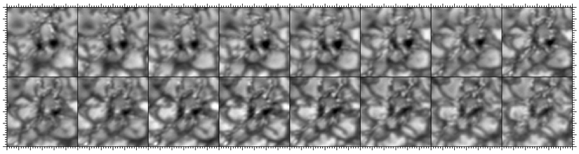
Figure 7: Temporal evolution of micro-pores shown at 34-second intervals starting at 08:07 UT (top-left to bottom-right). The ROI is $6\arcsec\times 6\arcsec$ as indicated by the white square in Fig. 1. Major tick marks are separated by one arcsecond. All images are from the reconstructed broadband channel and are displayed in the same intensity range of 0.75 – 1.35 $I_{0}$.

4.1 Temporal evolution of micro-pores

A region-of-interest (ROI) with a size of $6\arcsec\times 6\arcsec$ centered on the micro-pores (white square in Fig. 1) is chosen to illustrate the temporal evolution of these structures in Fig. 7. The time sequence starts at 08:07 UT, the cadence is $\Delta t=34$ s, and the total duration of the time sequence is about $\Delta T\sim$10 min.

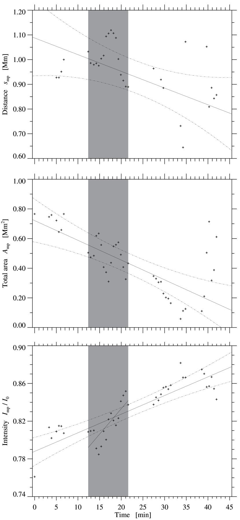
Figure 8: Chronological sequence of parameters describing the decay process of the micro-pores starting at 07:54 UT, i.e., center-to-center distance of the micro-pores $s_{\mathrm{mp}}$, total area $A_{\mathrm{mp}}$, and average intensity $I_{\mathrm{mp}}/I_{0}$ (top to bottom). The gray background indicates the 17 sequences with the best seeing conditions. The solid lines are linear fits to the parameters, and the dash-dotted lines represent the 3$\sigma$-error margins.

Initially, two micro-pores are present with diameters of less than $1\arcsec$, which evolve with time in intensity, size, and shape. The right micro-pore is circular, whereas the left micro-pore exhibits some star-like extrusions. The intensity of both micro-pores gradually increases, and at the same time the area decreases. As well as the term ‘micro-pore’, Rouppe van der Voort et al. (2005) introduced the nomenclature ‘ribbon’ and ‘flower’ for elongated and more circular magnetic structures, respectively, to capture their morphology at sub-arcsecond scales. The transition from flower to ribbon begins for the left micro-pore early-on in the time series, whereas the right micro-pore maintains its perceptual structure for about three minutes and then makes the transition from flower to ribbon. Small-scale brigthenings and signatures of abnormal granulation (de Boer & Kneer, 1992) are present everywhere in the vicinity of the micro-pores (e.g., near the coordinates (30″, 30″) and (29″, 21″) in Fig. 1).

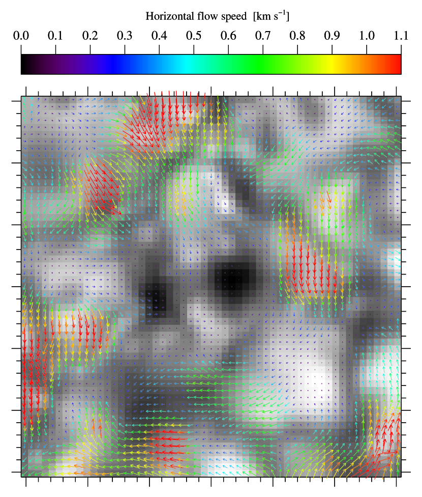
Figure 9: Horizontal proper motions in the vicinity of the two micro-pores. Color-coded arrows indicate magnitude and direction of horizontal flows for each pixel of the first broad band image shown in Fig. 7, an enlarged version of which serves as the background. Major tick marks are separated by one arcsecond. The FOV $6\arcsec\times 6\arcsec$ as indicated by the white square in Fig. 1.

The ten-minute time series in Fig. 7 displays the two micro-pores under the best seeing conditions. However, the other three time series also contain moments of good seeing, thus allowing us to study the evolution of the micro-pores more quantitatively over a period of about 40 minutes. Smoothing using anisotropic diffusion (Perona & Malik, 1990), intensity thresholding ($<0.9\,I_{0}$), and standard tools for ‘blob analysis’ (Fanning, 2011) yield the area of the micro-pores, their intensity distribution, and their center coordinates, which in turn provide the distance between the micro-pores. A more detailed description of this procedure is given in Verma & Denker (2014). The temporal evolution of the total area $A_{\mathrm{mp}}$ of the micro-pores, their average intensity $I_{\mathrm{mp}}$ given in terms of the quiet-Sun intensity $I_{0}$, and the center-to-center distance $s_{\mathrm{mp}}$ are presented in Fig. 8. Because the micro-pores evolve in a dynamic environment, being constantly jostled around by granules, they change shape and sometimes even seem to merge or split (mediocre seeing also affects the feature identification). Therefore, only data points are included for the distance, where the two micro-pores can be clearly identified. In addition, some restored broadband images were omitted because of mediocre seeing conditions.

All aforementioned parameters indicate the photometric decay of the system of micro-pores; the total magnetic flux of the EFR, however, remains constant but its distribution within the region changes. At the beginning of the sequence the micro-pores are about 1.1 Mm apart, have a total area of around 0.8 Mm², and their average intensity is just $0.75\,I_{0}$. Linear least-squares fits establish that the two micro-pores approach each other with a speed of $ds_{\mathrm{mp}}/dt=-0.11$ km s^-1, shrink at a rate of $dA_{\mathrm{mp}}/dt=-0.22$ km² s^-1, and approach quiet-Sun intensity levels at $dI_{\mathrm{mp}}/dt=0.033\,I_{0}$ s^-1.

Measuring the magnetic flux and thus the growth and decay rates is hampered by the low cadence (96 min), the varying noise level as a function of the heliocentric angle, the geometric foreshortening of the pixel area, the angle of the magnetic field lines (assumed to be perpendicular to the surface) with the line-of-sight (LOS), and the small number of pixels having a flux density of more than 20 G. Therefore, we conservatively report only the total unsigned magnetic flux of $2.2\times 10^{20}$ Mx (the negative magnetic flux is $1.2\times 10^{20}$ Mx) at 08:00 UT on 2008 August 7, which attains a maximum right at the time of the high-resolution GFPI observations. The flux contained in the EFR is slightly larger than the upper limit for ephemeral regions (see van Driel-Gesztelyi & Green, 2015), that is, much too small to form larger pores or even sunspots. Even though the time resolution is too coarse to provide a growth rate for the magnetic field, our measurements agree with a rapid rise time (already significant changes between the first two magnetograms) and a much slower decay rate (total unsigned flux of $1.3\times 10^{20}$ Mx at 22:24 UT on 2008 August 7). However, we cannot use the MDI continuum images to determine the lifetime of the micro-pores because their size is only a small fraction of an MDI pixel.

The $3\sigma$-errors given in Fig. 8 demonstrate that a linear model for the decay process of the micro-pores is in general appropriate – at least for the time interval under study. However, there are some deviations, in particular during the time with the best seeing (highlighted gray area in Fig. 8), where a more detailed inspection is warranted. The two micro-pores start to separate, while becoming darker. During this period the left micro-pore almost vanishes while the one on the right changes its shape from roundish to more elongated. Toward the end of the sequence shown in Fig. 7, the left micro-pore slowly recovers. A linear least-squares fit for just this time period yields an increased intensity gradient of $dI_{\mathrm{mp}}/dt=0.045\,I_{0}$ s^-1. The increase in total area toward the end of the sequence is caused by newly forming and merging micro-pores. A slight decrease in intensity accompanies this emergence process, as expected for a small-scale magnetic flux kernel with increasing magnetic flux. Taking the temporal derivatives $ds_{\mathrm{mp}}/dt$, $dA_{\mathrm{mp}}/dt$, and $dI_{\mathrm{mp}}/dt$ at face value leads to the conclusion that the decaying micro-pores will vanish before merging.

4.2 Horizontal flow field around micro-pores

Magnetic field concentration are known to influences horizontal proper motions. We used LCT (Verma & Denker, 2011) to investigate if even micro-pores potentially impact the surrounding plasma motions. The mean flow speed is $\bar{v}=0.59\pm 0.41$ km s^-1 across the entire FOV and $\bar{v}=0.49\pm 0.31$ km s^-1 in the ROI shown in Fig. 9. In both cases, the standard deviation refers to the variation within the observed field rather than to a formal error estimate. The corresponding 10^th percentiles of the speed distributions are $v_{10}=1.15$ and 0.93 km s^-1, respectively. These values are slightly higher than those provided in Fig. 7 of Verma et al. (2013). However, considering the shorter averaging time of $\Delta T\approx 10$ min as compared to $\Delta T=60$ min for Hinode G-band images, the LCT results are in good agreement with the values presented by Verma et al. (2013).

Neither inflows nor outflows surround the two micro-pores. The flow field is still dominated by the jostling motion of the solar granulation. As already noted in Verma & Denker (2011), much longer averaging times are needed to clearly detect persistent flows. However, the flow speed is significantly reduced in the immediate surroundings of the micro-pores ($\pm$1″). Detecting (micro-) pores at spatial scales of one arcsecond or below is a formidable task. In their extensive statistical study based on Hinode data, Verma & Denker (2014) consequently required an area of at least 0.8 Mm² for pores to be included in the sample, which would exclude the two micro-pores depicted in Fig. 9. Therefore, this case study provides additional information for the smallest features that can still be considered to be pores.

4.3 Chromospheric fine structure and Doppler velocity

Both the H$\alpha$ line-core intensity (bottom panel in Fig. 1) and the H$\alpha$ Doppler velocity maps (Fig. 10) reveal the rich fine structure of the solar chromosphere. The center-of-gravity method (Schmidt et al., 1999) is very efficient and robust in retrieving the H$\alpha$ Doppler velocities. Repeating the white rectangle and square already drawn in Fig. 1 facilitates easy comparison with the photospheric observations – in particular, the rectangle validates the choice of the quiet-Sun region as the Doppler velocity reference, because this region is free of any chromospheric filamentary structure and does not exhibit any peculiar chromospheric flows; and the square illustrates the association of the micro-pores with H$\alpha$ brightenings and strong downflows in excess of 6 km s^-1 near the footpoints of small-scale H$\alpha$ loops belonging to the AFS. However, the Doppler velocities are close to zero at the exact location of the micro-pores.

The AFS consists of two regions with H$\alpha$ line-core brightenings. Some small-scale loops connect these areas containing the bipolar EFR. Other loops rooted in the bright patches connect to the outside of the EFR. Some bright fibrils are interspersed among the dark filaments. The width of the loops is just a few seconds of arc, and their length is about 6″ – 8″. Typical aspect ratios for the dark filaments are 1 : 4 to 1 : 5. The morphology of the micro-pores, the EFR, and the small AFS closely resembles structures reported in other studies (e.g., Strous et al., 1996; Tziotziou et al., 2003; Wedemeyer-Böhm et al., 2009; Zuccarello et al., 2009). The cross-shaped markers labeled a – f identify the locations of some exemplary H$\alpha$ contrast profiles, for example, labels c and d refer to a dark arch filament and a footpoint, respectively. Properties and parameters derived from CM inversions of the contrast profiles are discussed in Sect. 4.5.

H$\alpha$ Doppler velocities $v$ are computed for the dark filaments of the AFS and the bright footpoint areas. Intensity and size thresholds in combination with morphological image processing of the H$\alpha$ line-core intensity maps yield binary masks of bright and dark features. Indexing of pixels belonging to these areas facilitates computing histograms for dark filamentary features ($n=7009$ pixels) and bright footpoints ($n=2827$ pixels) shown in the left and right panels of Fig. 11, respectively. The histogram of the dark filamentary features is characterized by a median value of $v_{d,\mathrm{med}}=-0.10$ km s^-1, a mean value of $\bar{v}_{d}=-0.13$ km s^-1, and a standard deviation of $\sigma_{d}=1.31$ km s^-1. The corresponding values for the bright footpoints are $v_{b,\mathrm{med}}=3.77$ km s^-1, $\bar{v}_{b}=3.97$ km s^-1, and $\sigma_{b}=1.86$ km s^-1.

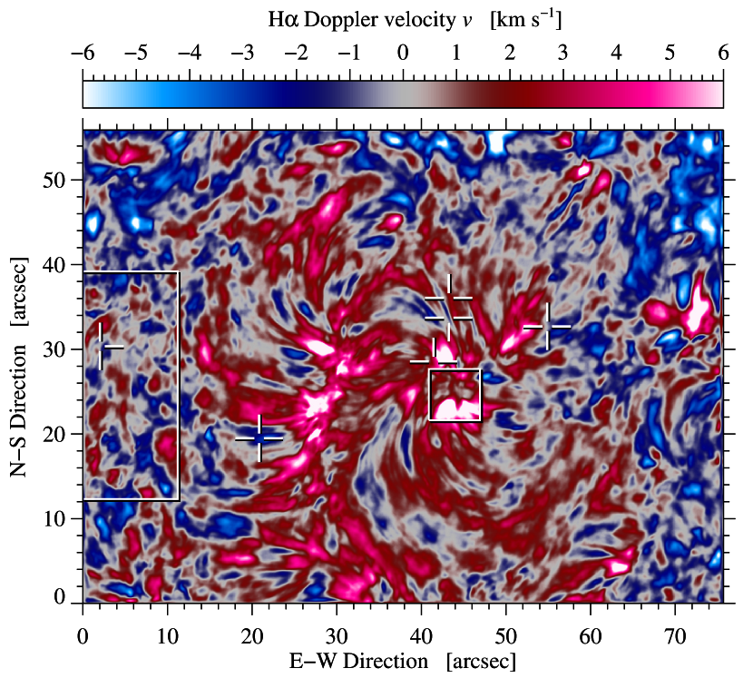
Figure 10: Chromospheric Doppler velocity map corresponding to Fig. 1 derived with the center-of-gravity method. Blue and red colors represent up- and downflows, respectively.

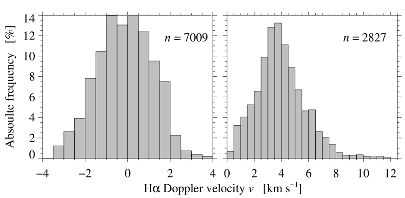
Figure 11: Normalized histograms of the chromospheric Doppler velocities $v_{d}$ for dark filamentary features (left) and $v_{b}$ for bright footpoints (right) of the small AFS in Figs. 1 and 10. The variable $n$ indicates the number of H$\alpha$ line profiles on which the distributions are based.

Both up- and downflows occur in the dark filaments with a small imbalance toward blueshifts. Notwithstanding, the bright footpoint regions almost exclusively harbor downflows with velocities as high as 12 km s^-1. Interestingly, blue- and redshifted H$\alpha$ profiles appear in close proximity along the loops (see labels e and f), which can be interpreted as up- and downflows. However, counter-streaming and even rotation along the filament axis are possibilities depending on the specific three-dimensional loop topology. The typical mean upflow velocity at the loop tops is $\bar{v}_{lt}=-1.13$ km s^-1, and extreme values approach $v_{lt,\mathrm{max}}=-3$ km s^-1. In general, the ratio of the area between up- and downflowing cloud material is $A_{\mathrm{up}}/A_{\mathrm{down}}=0.22$.

4.4 Cloud model inversions

Table 1: Mean value and standard deviation of CM parameters for the quiet Sun, the dark filamentary features, and all fitted contrast profiles.

		quiet Sun	dark filaments	all profiles
$S$		$0.14\pm 0.07$	$0.12\pm 0.02$	$0.15\pm 0.05$
$\Delta\lambda_{D}$	[pm]	$30.44\pm 10.36$	$41.62\pm 7.17$0	$33.96\pm 10.74$
$\tau_{0}$		$0.44\pm 0.30$	$1.19\pm 0.45$	$0.85\pm 0.53$
$v_{\mathrm{LOS}}$	[km s-1]0	0$-1.41\pm 10.16$$-$	$-0.94\pm 3.84$$-$	$0.41\pm 8.61$

Table 2: Gaussian and log-normal fit parameters of the normalized histograms of the CM parameters shown in Fig. 14.

		$\mu_{1}$	$\sigma_{1}$	$\mu_{2}$	$\sigma_{2}$	$P_{1}$
$S$		$0.14$	$0.02$	$0.18$	$0.01$	$0.83$
$\Delta\lambda_{D}$	[pm]	$25.92$0	$6.81$	$42.09$0	$6.35$	$0.54$
$\tau_{0}{{}^{\dagger}}$		$0.17$	$3.5$	$1.00$	$2.60$	$0.50$
$v_{\mathrm{LOS}}$	[km s-1]	$0.61$	$9.77$	$0.39$	$3.45$	$0.76$

^†Two Gaussians are fitted to the normalized histograms of the CM fit parameters with the exception of $\tau_{0}$, where the fit consists of a two log-normal distributions.

The rms-deviation between observed and inverted contrast profiles is taken as an additional criterion to select only the best-matched profiles (60% of the entire FOV) as shown in Fig. 12, where mediocre fits are excluded and indicated as light gray areas. Rejected regions include much of the quiet Sun and the micro-pores including the surrounding regions with H$\alpha$ line-core brightenings. In all cases, the underlying assumption of CM inversions is not valid, that is, the premise of cool absorbing plasma suspended by the magnetic field above the photosphere does not apply. Mean values and standard deviations of the CM fit parameters are summarized in Table 1 for the quiet-Sun region indicated by the white rectangles in Figs. 1 and 10, the dark filamentary features, and all fitted profiles. The dark filamentary features represent just 2% of all contrast profiles in the image.

In all three cases, the source function $S$ is virtually the same, except for the lower standard deviation of the dark filamentary features. The Doppler width $\Delta\lambda$ and the optical thickness $\tau_{0}$ are significantly larger in the dark filamentary features as compared to quiet-Sun regions. The dark features show on average a small upflow similar to the quiet Sun. The quiet-Sun LOS velocity $v_{\mathrm{LOS}}$ is not zero like the H$\alpha$ Doppler velocity $v$, which is likely a selection effect because CM inversions are not available for all pixels of the reference region. The LOS velocity $v_{\mathrm{LOS}}$ for the entire FOV is slightly redshifted because of the downflows encountered in the EFR and AFS. The small standard deviation of all CM fit parameters for the dark filamentary features indicates that they belong to a specific class of absorption features.

Table 3: Results of cluster analysis for the CM parameters depicted in in Figs. 14 and 12.

2 populations		$w_{1}$	$w_{2}$	$w_{3}$	$w_{4}$	$\mu_{1}\pm\sigma_{1}$	$\mu_{2}\pm\sigma_{2}$	$\mu_{3}\pm\sigma_{3}$	$\mu_{4}\pm\sigma_{4}$
$S$		$0.15$	$0.15$			$0.13\pm 0.04$	$0.15\pm 0.04$
$\Delta\lambda_{D}$	[pm]	$16.00$0	$47.00$0			$23.96\pm 4.98$0	$41.54\pm 5.57$0
$\tau_{0}$		$0.31$	$0.33$			$0.66\pm 0.45$	$1.02\pm 0.52$
$v_{\mathrm{LOS}}$	[km s-1]	$-7.03$0	$-6.29$0			0$0.67\pm 10.58$	$0.19\pm 5.84$
Cluster fraction		$c_{1}=43.4$%	$c_{2}=56.6$%
3 populations
$S$		$0.14$	$0.15$	$0.15$		$0.13\pm 0.05$	$0.13\pm 0.04$	$0.15\pm 0.04$
$\Delta\lambda_{D}$	[pm]	$20.18$0	$16.80$0	$47.50$		$24.99\pm 5.15$0	$25.37\pm 6.19$0	$42.30\pm 6.52$0
$\tau_{0}$		$0.36$	$0.34$	$0.32$		$0.56\pm 0.39$	$0.72\pm 0.48$	$1.04\pm 0.52$
$v_{\mathrm{LOS}}$	[km s-1]	$-16.04$00	$10.09$0	$-6.14$0		$-11.18\pm 5.34$00	$7.79\pm 5.88$	$-0.71\pm 4.78$0
Cluster fraction		$c_{1}=16.2$%	$c_{2}=33.0$	$c_{3}=50.8$%
4 populations
$S$		$0.14$	$0.15$	$0.15$	$0.16$	$0.13\pm 0.05$	$0.13\pm 0.04$	$0.16\pm 0.04$	$0.15\pm 0.03$
$\Delta\lambda_{D}$	[pm]	$19.73$0	$16.67$0	$48.55$0	$39.71$0	$23.72\pm 4.98$0	$23.81\pm 5.47$0	$49.43\pm 4.30$0	$37.03\pm 4.91$0
$\tau_{0}$		$0.32$	$0.31$	$0.30$	$1.18$	$0.50\pm 0.36$	$0.67\pm 0.47$	$1.06\pm 0.55$	$1.00\pm 0.50$
$v_{\mathrm{LOS}}$	[km s-1]	$-16.38$00	$10.20$0	$-5.51$0	$-4.75$0	$-12.33\pm 5.18$00	$8.31\pm 6.10$	$-0.41\pm 4.72$0	$-0.62\pm 5.48$0
Cluster fraction		$c_{1}=43.1$%	$c_{2}=17.2$%	$c_{3}=27.3$%	$c_{4}=12.4$%

The cluster analysis was performed for $k=2$, 3, and 4 populations. The weights $w_{i}$ refer to the cluster centers. In addition, mean values $\mu_{i}$ along with the standard deviations $\sigma_{i}$ were computed for the CM parameters of each cluster. The cluster fractions $c_{i}$ are given with respect to all good CM fits.

4.5 Properties of the arch filament system

The results of the CM inversions are presented in Fig. 12 for the parameters source function $S$, Doppler width $\Delta\lambda_{D}$, optical thickness $\tau_{0}$, and LOS velocity of the cloud material $v_{\mathrm{LOS}}$, which is not the same as the Doppler velocity $v$ obtained with the center-of-gravity method. The linear correlation coefficient between these two quantities is $\rho(v_{\mathrm{LOS}},\,v)=0.80$. The linear regression model can be written as $v=c_{0}+c_{1}\cdot v_{\mathrm{LOS}}$ with the constants $c_{0}=0.20$ km s^-1 and $c_{1}=0.15$. The linear correlation of $v_{\mathrm{LOS}}$ and $v$ reduces to $\rho_{lt}=0.73$ and $\rho_{qs}=0.64$ for specific features such as loop tops and the quiet Sun.

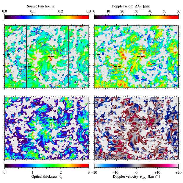
Figure 12: Maps of CM parameters for the inverted H$\alpha$ contrast profiles corresponding to Fig. 1, i.e., source function $S$, Doppler width $\Delta\lambda_{D}$, optical thickness $\tau_{0}$, and LOS velocity $v_{\mathrm{LOS}}$ (top-left to bottom-right). Light gray areas indicate regions, where the CM inversions did not deliver good fits. The two white vertical lines in the upper-left panel enclose the ROI, which was selected to show the evolution of the AFS in Fig. 13. The FOV is the same as shown in Fig. 1.

The parameters $S$, $\Delta\lambda_{D}$, and $\tau_{0}$ reach their largest values in proximity to the H$\alpha$ line-core brightenings. In regions, which are free of any filamentary structure, the values for this set of parameters are much lower. The velocity $v_{\mathrm{LOS}}$ within the EFR and the AFS is predominantly directed downwards with the exception of the loop tops of the dark filamentary features, where significant upflows arise, which are clearly in excess of the H$\alpha$ Doppler velocity $v$ (compare with Fig. 1).

The temporal evolution of selected CM parameter maps is shown in Fig. 13 for the central ROI containing the EFR and AFS as indicated in the top-left panel of Fig. 12. The first row corresponds to Fig. 12 at 08:07 UT, whereas the other rows display maps at 136-second intervals (every fourth image in Fig. 7). The CM inversions and the quiet-Sun selection follow the same procedure as for the first CM map. The backgrounds of source function $S$ and optical thickness $\tau_{0}$ remain very stable but changes of their extreme values closely track the evolution of the dark arch filaments. The Doppler width $\Delta\lambda_{D}$ of the arch filaments reaches a maximum in the third map. The velocity $v_{\mathrm{LOS}}$ at the loop tops reveals upflows in the first three maps while in the last two maps downflows appear at the same position. This points to the very dynamic nature of AFSs. Despite individual active features, in particular the loop tops, on the whole the AFS is very stable over the 10-minute time series, which is consistent with the results of Tsiropoula et al. (1992).

Normalize histograms for all CM parameters are given in Fig. 14. The distributions for source function $S$ and optical thickness $\tau_{0}$ show a conspicuous ‘shoulder’ on the right side, the one for the Doppler width $\Delta\lambda_{D}$ is double-peaked, and the one for the velocity $v_{\mathrm{LOS}}$ possess an extended base. All these characteristics are indicative for a sample with two (or more) distinct populations, for example, quiet Sun and AFS. In general, the frequency of occurrence is well represented by two Gaussians ($S$, $\Delta\lambda_{D}$, and $v_{\mathrm{LOS}}$). Only in case of the optical thickness $\tau_{0}$, two log-normal distributions are a more appropriate model. The mean values $\mu_{1,2}$ and standard deviations $\sigma_{1,2}$ of the fit parameters (or the parameter’s natural logarithm for $\tau_{0}$) are given in Table 2 along with the normalized frequency of occurrence $P_{1}$ of the dominant population.

The histograms provide indirect evidence that two features with distinct CM parameters are present within the observed FOV. However, they do not offer hints, where these features are located, because the distributions strongly overlap. Cluster analysis offers a variety of statistical tools to identify distinct populations in an $n$-dimensional parameter space. In our case this means the four-dimensional space of CM parameters (see Figs. 14 and 12). The number of samples in each histogram is $m=200\,188$. The $k$-means clustering algorithm implemented in IDL (Everitt et al., 2011) requires a priori knowledge about the number of clusters $k$. The histograms favor $k=2$. However, the cases $k=3$ and $k=4$ are also investigated to validate that two distinct populations are indeed sufficient to represent the data. The clustering algorithms assigns the samples to a cluster such that the squared distance from the cluster center is minimized and the distance between the cluster centers is maximized. The clustering algorithm provides additional information to explain the different shapes observed in the histogram of Fig. 14, meaning two peaks for the Doppler width $\Delta\lambda_{D}$, the halo for the LOS velocity $v_{\mathrm{LOS}}$ and the shoulders for the optical thickness$\tau_{0}$ and the source function $S$.

Cluster centers or weights $w_{i}$ are not necessarily the same as the mean values $\mu_{i}$ of the clusters because of the above optimization scheme. In addition to the mean values $\mu_{i}$, we list in Table 3 the respective standard deviations $\sigma_{i}$ to illustrate the extend and potential overlap of the clusters. The size of each population is given by the cluster fraction $c_{i}$, and the normalized histograms for all the CM parameters are given in Fig. 15 for the case $k=2$.

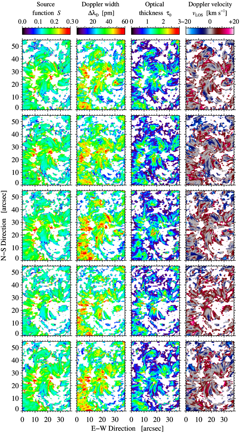
Figure 13: Temporal evolution of CM parameters (top to bottom) for the ROI containing the EFR and AFS. The maps are depicted at 136-second intervals starting at 08:07 UT (see Fig. 12) and show source function $S$, Doppler width $\Delta\lambda_{D}$, optical thickness $\tau_{0}$, and LOS velocity $v_{\mathrm{LOS}}$ (left to right). The two white vertical lines in the upper-left panel shown in Fig. 12 enclose the FOV of this figure.

In the case of just two populations, the Doppler width of the absorption profiles $\Delta\lambda_{D}$ has the strongest discriminatory power. These broad absorption profiles also have a higher optical thickness $\tau_{0}$. On the whole, the mean values and standard deviations of the other CM parameters are very similar with the exception of the larger standard deviation $\sigma_{1}$ for the velocity $v_{\mathrm{LOS}}$. This broader distribution is also easily perceived in Fig. 15. In general, there is a good agreement between the distributions in Figs. 14 and 15. Only a secondary peak for the source function $S$ of cluster $c_{1}$ and the strong deviation from a log-normal distribution of the the optical thickness $\tau_{0}$ of the cluster $c_{2}$ point to the presence of more than two populations. The cluster fractions of $c_{1}=43.3$% and $c_{2}=56.6$% are very similar, which however might be related to the $k$-means clustering algorithm’s tendency to produce clusters of similar size.

Increasing the number of clusters to $k=3$ splits the population according to the velocity $v_{\mathrm{LOS}}$ into up- and downflows, while at the same time populations 1 and 2 maintain a similar Doppler width $\Delta\lambda_{D}$ as before. Increasing the number of clusters to $k=4$, population 3 for the case $k=3$ separates into populations 3 and 4 according to the Doppler width, which is still significantly larger than for populations 1 and 2. In summary, increasing successively the number of clusters from $k=2$ to $k=4$, first forks population 1 into up- and downflows and then branches population 2 into contrast profiles with narrower and broader Doppler width $\Delta\lambda_{D}$. However, we conclude that two populations are sufficient to represent the distributions of the CM parameters, which are most easily distinguishable by the Doppler width $\Delta\lambda_{D}$ and to a lesser extend by the optical thickness $\tau_{0}$ of the cloud material. More than two populations likely overinterpret the data because they cannot be associated with any particular chromospheric feature.

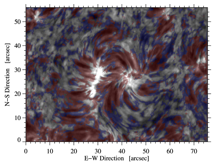
Figure 16: Two-dimensional map containing the locations of the two clusters $c_{1}$ (blue) and $c_{2}$ (red), which were identified in the cluster analysis assuming that the histograms of the CM parameters contain only two distinct populations. The H$\alpha$ line-core intensity image of Fig. 1 serves as the background. The gray areas indicate the same regions as in Fig. 12, where the CM inversions result in mediocre fits.

The locations of the two populations are depicted in Fig. 16 in blue and red colors, whereas the gray areas indicate the same regions as in Fig. 12 with mediocre CM fits. The background of the figure is the H$\alpha$ line-core intensity image presented in Fig. 1 to assist in matching the two populations to chromospheric features. Population 1 (blue) marks the transition to the quiet Sun, where the cloud material turns more transparent, that is, $\Delta\lambda_{D}$ and $\tau_{0}$ become increasingly smaller. Population 2 (red) is thus more representative for the small AFS, and the corresponding CM parameters in Tables 2 and 3 should be used in comparisons to values provided in literature. To ensure that these two populations are not some artifacts of the CM inversions, we examine their $\chi^{2}$ statistics. The mean values along with their standard deviations are $\chi^{2}_{1}=0.064\pm 0.040$ and $\chi^{2}_{2}=0.048\pm 0.033$, which are essentially the same.

Figure 14: Normalized histograms of the CM parameters (dotted) depicted in Fig. 12. The dashed and dash-dotted curves are double Gaussian fits with an exception for $\tau_{0}$, where two log-normal distributions replace the two Gaussians. The solid curves correspond to the sum of the fitted distributions.

5 Discussion

In this study, we analyze a short period in the evolution of the photospheric and chromospheric signatures belonging to a small EFR containing two micro-pores and a small AFS, where significant changes take place in just a few tens of minutes. These micro-pores with sizes of less than one arcsecond, as seen at photospheric level, are evolving with time in intensity, shape, and size. Their average intensity increased and concurrently the total area decreased, which we interpret as a signature of a local decaying process. Fade-out and disintegration of strong magnetic elements is also supported by the presence of small-scale continuum brigthenings and transient signatures of abnormal granulation (de Boer & Kneer, 1992) in the vicinity of the micro-pores. The shape of the micro-pores evolves as first reported by Rouppe van der Voort et al. (2005) - alternating between ribbons and flowers. These authors ascribe the dynamics of micro-pores to a fluid-like behavior of magnetic flux, which they relate to magnetic features evident in magneto-hydrodynamic simulations (e.g., Carlsson et al., 2004; Vögler et al., 2005), see also Beeck et al. (2015) for more recent simulation results. At very high spatial and temporal resolution, the present study confirms the overall picture of the evolution of magnetic concentrations as presented by Schrijver et al. (1997), among others, in which (micro-)pores can split, merge, or vanish.

The temporal derivatives of the mean total area ($dA_{\mathrm{mp}}/dt=-0.22$ km² s^-1) and the average intensity ($dI_{\mathrm{mp}}/dt=0.033\,I_{0}$ s^-1) can be boundary conditions of magnetohydrodynamic simulations on flux emergence in general and particularly in solar pore formation (e.g., Stein et al., 2011; Stein & Nordlund, 2012; Cameron et al., 2007; Rempel & Cheung, 2014). Even if the statistical values in the present study only represent the evolution of one set of micro-pores, the initial mean intensity $0.75\,I_{0}$ and size 0.8 Mm² are consistent with other observations and simulations. The size dependence of the brightness was reported before in observations and simulations (e.g., Cameron et al., 2007; Bonet et al., 1995; Keppens & Martinez Pillet, 1996; Mathew et al., 2007). Small pores are not as dark as larger ones. The brightness increases when pores decay, and they contract and lose flux (Cameron et al., 2007). These authors suggest that increasing lateral radiative heating reduces the pore’s size. This effect is compounded by the irregular shape of decaying pores.

The LCT results of horizontal flow field around the micro-pores agree quantitatively with Verma & Denker (2011). However, the short-averaging time implies that the flow speeds more closely reflect motions of individual granules, dark micro-pores, and small-scale brightenings. Persistent flows become only apparent with longer averaging times (Verma et al., 2013). Yet, the significantly reduced flow speed in the micro-pores clearly indicates that the magnetic field is sufficiently strong to suppress the convective motions in close proximity to the micro-pores and to cancel horizontal motions inside the two H$\alpha$ line-core brightenings (see Fig. 9).

The statistical description of micro-pores is still inadequate and limited to pores with diameters of about 1 Mm, even when resorting to high-resolution Hinode data (Verma & Denker, 2014). In addition, advanced simulations of emerging bipolar pore-like features (e.g., Stein et al., 2011) use larger boxes (about 50 Mm wide) with larger pores (about 10 Mm diameters) and larger separations of the bipoles (about 15 Mm), i.e., they do not necessarily capture the physics and dynamics of micro-pores at sub-arcsecond scales. The observed micro-pores are ‘isolated’ pores, which represent about 10% of the pore population (Verma & Denker, 2014). Isolated pores may have their origin in a solar surface dynamo (Vögler & Schüssler, 2007). Therefore, (micro-)pores in the quiet Sun and in active regions are potentially due to different dynamo actions.

The H$\alpha$ line-core intensity, Doppler velocity maps and MDI magnetograms reveal a chromospheric arch filamentary structure with two regions of H$\alpha$ line-core brightenings and small loops connecting these two areas in a bipolar region with opposite polarities. A similar region was also described in Harvey & Martin (1973). The width of the dark filaments is a few seconds of arc, and their length is around 6 – 8″, which is smaller than the mean lengths reported by Tsiropoula et al. (1992). We find typical aspect ratios of the loops of between 1:4 and 1:5. Overall, but with smaller spatial dimensions, the morphology of the observed AFS agrees with the findings reported in several studies (e.g., Strous et al., 1996; Tziotziou et al., 2003; Wedemeyer-Böhm et al., 2009; Zuccarello et al., 2009).

Figure 15: Normalized histograms of the CM parameters based on cluster analysis with the same data as in Fig. 12. The dashed and dash-dotted curves refer to the two clusters $c_{1}$ and $c_{2}$, respectively.

The H$\alpha$ Doppler velocity $v$ at the bright footpoints is mainly downwards with a flow speed of up to 12 km s^-1. The up- and downflows in the dark filamentary system possess an imbalance toward blueshifts with typical mean upflow velocities of $\bar{v}_{LT}\approx-1.13$ km s^-1 at the loop tops, but some upflows reach values close to $-3$ km s^-1. Furthermore, the close proximity of some up- and downflows taken together with their appearance in time-lapse movies support the presence of twisting motions along the loop axis. Many other spectroscopic or spectropolarimetry studies have observed AFS in the chromospheric absorption line H$\alpha$ and in the Ca ii H & K lines (Bruzek, 1969; Zwaan, 1985; Chou & Zirin, 1988; Lites et al., 1998). The range of the downflow Doppler velocities $v$ near the footpoints spans 30 – 50 km s^-1, whereas upflows of about 1.5 – 22 km s^-1 are observed at the loop tops.

In general, the velocities in the present study are much lower than those reported by the aforementioned authors. This can be attributed to the smaller size of the loop system as compared to previous studies. The higher the velocities, the higher the size of the loop systems. The small and isolated upflow patches in the present study are closer to the Doppler velocities reported in Lites et al. (1998) with observations near the disk center. They suggest that the observed AFS is not caused by a monolithic flux rope but the result of the dynamical emergence of a filamentary flux bundle. The most accepted flux emergence scenario suggest that the EFRs are formed by magnetic flux tubes that are transported from the base of the solar convection zone (tachocline) to the solar surface by buoyancy (Zwaan, 1987). Normally, these emerging field appears on the solar surface in form of bipolar regions as in our observations known as EFR. The two polarities are commonly the footpoints of an $\Omega$-loops system rising to the solar surface even up to the solar corona (e.g., Schmieder et al., 2004; Strous & Zwaan, 1999; Strous et al., 1996) Furthermore, at chromospheric level, flows occur within the AFS accompanied by draining material from the H$\alpha$ loops toward the footpoints, where the higher downflows reside. In the case of Lites et al. (1998), this occurs where pores and sunspots form. In our case, only one footpoint shows an intensity signature - micro-pores evolving in the photosphere. Another explanation of the physical processes in loops connecting the two footpoints is an upflow that starts in the middle of two regions with opposite magnetic flux, in our case, in the middle and upper part of the two footpoints (magnetic configuration of the case C in Fig. 12 of Lee et al. (2000). The origin of the upflow events is then explained by magnetic reconnection. The mass moves upward through the small loops and falls down in other areas far away.

We have presented maps of four CM parameters and the corresponding normalized histograms based on CM inversions of H$\alpha$ contrast profiles (Figs. 14 and 12), i.e., source function $S$, Doppler width $\Delta\lambda_{D}$, optical thickness $\tau_{0}$, and velocity of the cloud material $v_{\mathrm{LOS}}$. The inversion scheme provided well matched profiles for around 60% of the entire FOV. The population of the inverted AFS contrast profiles covered only about 2% of the entire FOV. Failed CM inversions are mainly related to much of the quiet-Sun regions and the H$\alpha$ line-core brightenings, where the underlying assumptions of the model are violated.

The inversion results for quiet-Sun regions, dark filamentary features, and the ensemble average show in general similar values. However, the Doppler width and the optical thickness of the dark chromospheric filaments are much larger than in the quiet-Sun regions, and the velocity $v_{\mathrm{LOS}}$ possesses, similar to the quiet-Sun regions, a small upflow on average. We note that the average quiet-Sun Doppler velocity is based on the center-of-gravity methods not the CM inversions. Furthermore, the velocity $v_{\mathrm{LOS}}$ of the entire FOV is on average redshifted because of the downflows being present in the EFR and the AFS, with the exception of the loop tops. In the CM maps it is clearly seen that the parameters $S$, $\Delta\lambda_{D}$, and $\tau_{0}$ reach the largest values in proximity to the H$\alpha$ line-core brightenings. In regions lacking any filamentary structure, the values are much lower. The results of the CM parameters in Table 2 are very similar to the ones presented by Bostanci (2011) for dark mottles. They are also close to the results of AFSs investigated by Alissandrakis et al. (1990), whereas the source function $S$ and optical thickness $\tau_{0}$ deviate from the results presented by Bostanci & Erdogan (2010); Lee et al. (2000).

The AFS in the present study certainly belongs to the smallest observed chromospheric filaments. Only mini-filaments (Wang et al., 2000) are smaller. Interestingly, the CM inversion results are similar as compared to a giant filament investigated by Kuckein et al. (2016). As expected, their mean optical thickness $\tau_{0}$ is larger than our average inferred values.

The normalized histograms suggest that the CM parameters represent two different populations, which is corroborated by the cluster analysis and the computed absolute contrast that clearly distinguishes between features with higher contrast belonging to the AFS and those being part of quiet-Sun regions or the interface between the quiet Sun and the AFS. We did expect that for similar observations with a small FOV containing AFSs two populations may appear again all over the solar disk and distinguish between dark AFS and the regions of the quiet-Sun and the transition to the quiet-Sun. We note that in several studies the authors select only region of interest, that is, the features with high contrast and they do not invert the quiet-Sun regions, (e.g., Kuckein et al., 2016; Contarino et al., 2009). For larger FOVs that may contain different features like active regions, filaments, quiet-Sun, rosette structures, etc., we foresee that CM inversions together with cluster analysis will separate these chromospheric features in different populations based on the four CM parameters.

6 Conclusions

Photospheric and chromospheric structures like sunspots and pores cover a broad range of spatial scales. Sunspots come into existence as pores, grow, and potentially assemble into large (complex) active regions. In the chromosphere, cool plasma is suspended by the magnetic field in structures ranging in size from mini-filaments (a few megameters) to giant and polar crown filaments (several hundred megameters). This raises the questions if scaling laws exist characterizing the physical properties of these phenomena. In EFRs with AFSs both photospheric and chromospheric properties are relevant. Exploring the lower end of their spatial scales requires large-aperture solar telescopes with dedicated instruments. As a consequence the observed FOV is small, time series cover at most a few hours, and synoptic observations building up a database are often impracticable. Therefore, case studies are the only means of advancing our knowledge of EFRs and AFSs at sub-arcsecond scales.

In the present study, we used the Göttingen Fabry-Pérot Interferometer to investigate a very small EFR with its accompanying AFS. It is almost inconceivable that systems with a clear bipolar magnetic structure exist that are smaller than this. Mini-filaments are not considered in this context because they reside at the polarity inversion line (PIL) between opposite magnetic polarities (Wang et al., 2000), thus representing a different magnetic field topology. In our observations, the AFS connects the micro-pores to a quiet-Sun region of opposite polarity flux, that is, the small-scale filaments are perpendicular to the PIL. The filaments or dark fibrils are a clear indication of a newly emerging flux in the form of $\Omega$-loops. The magnetograms represented in Fig. 2 show that the trailing polarity is formed earlier than the leading polarity and that it is formed earlier than the leading polarity. However, the leading polarity is more compact and survives longer. This asymmetry is a typical property of EFRs, also for larger ones (van Driel-Gesztelyi & Petrovay, 1990). The decay of the EFR is characterized by flux cancellation and fragmentation. The flux system emerged and then submerged as a whole similar to a larger EFR studied in Verma et al. (2016). Flux fragmentation indicate that several $\Omega$-loops and not just one monolithic loop connects the opposite polarities, which is also reflected in the multiple dark fibrils constituting the AFS.

The statistical description of micro-pores and flux emergence at spatial scale below 1 Mm remains challenging. We presented, among others, evolution timescales for the area of micro-pores, their mean intensity, and the separation of footpoints, which match previous observations and simulations, when taking into acount the size of the observed EFR and AFS. In the chromosphere, upflows are mainly observed at the loop tops and from there the cool plasma drains toward the footpoints. Generally, the LOS velocities inferred in the loops are two to four times lower than for larger AFSs. Buoyancy and curvature of the rising or submerging $\Omega$-loops is here the determining factor but a statistically more meaningful sample is clearly needed to derive scaling laws. Pores occur on spatial scales ranging from sub-arcsecond to about ten arcseconds. Thus, comparing observations of EFRs and AFSs in this spatial domain with simulations of flux emergence and decay will be very beneficial for our understanding of the dynamic interaction of magnetic fields with the surrounding plasma.

A shortcoming of the present study was the lack of high-resolution spectropolarimetric observations, which motivates follow-up observations with the GREGOR Fabry-Pérot Interferometer (GFPI, Puschmann et al., 2012) and the GREGOR Infrared Polarimeter (GRIS, Collados et al., 2012) at the 1.5-meter GREGOR solar telescope (Schmidt et al., 2012). Both instruments are capable of full-Stokes polarimetry and allow multi-wavelength observations of multiple spectral lines (e.g., H$\alpha$ with the GFPI and the spectral region around the He i triplet at 1083 nm with GRIS). In addition to magnetic field information, the height dependence of physical properties in EFRs and AFSs becomes thus accessible.