On the role of dealing with quantum coherence in amplitude amplification

Abstract

Amplitude amplification is one of primary tools in building algorithms for quantum computers. This technique generalizes key ideas of the Grover search algorithm. Potentially useful modifications are connected with changing phases in the rotation operations and replacing the intermediate Hadamard transform with arbitrary unitary one. In addition, arbitrary initial distribution of the amplitudes may be prepared. We examine trade-off relations between measures of quantum coherence and the success probability in amplitude amplification processes. As measures of coherence, the geometric coherence and the relative entropy of coherence are considered. In terms of the relative entropy of coherence, complementarity relations with the success probability seem to be the most expository. The general relations presented are illustrated within several model scenarios of amplitude amplification processes.

I Introduction

The Grover search algorithm grover97 ; grover97a ; grover98 is one of fundamental discoveries that motivate quantum computations. Celebrated Shor’s results shor97 have led to numerous quantum algorithms for algebraic problems hama2006 ; hallg07 ; vandam2010 . The authors of loka2007 gave arguments that Grover’s and Shor’s algorithms are more closely related than one might expect at first. It was soon recognized that Grover’s algorithm is optimal for searching by queries to oracle bbbv97 ; zalka99 . Here, we invoke the oracle to evaluate any item, whereas database per se is not represented explicitly. Today, there exists a class of quantum algorithms inspired by the Grover algorithm patel2016 . Due to the broad applicability of search problems patel2016 , researchers have attempted to formulate building blocks of the algorithm as generally as possible. The original algorithm may be modified by changing phases in the rotation operations and replacing the intermediate Hadamard transform with arbitrary unitary one. In addition, quantum computing may start with an arbitrary initial distribution of the amplitudes. Details of generalized versions of the Grover algorithm were described in biham99 ; biham2000 ; biham2002 .

It is well known that entanglement is a key resource in quantum information processing. The quantum parallelism of Deutsch deutsch85 assumes to use entangled states of a quantum register. The results of the papers bpati2002 ; jozsa03 manifested that quantum speed-up without entanglement seems to be impossible. On the other hand, quantum computations are connected with only limited number of bases, in which states of the register are represented. In order to analyze the quantum computational speed-up, we should think about quantum correlations with respect to the computational basis. The problem of quantifying coherence at the quantum level is currently the subject of active researches bcp14 ; abc16 ; plenio16 ; fan2017 . Studies of the role of quantum coherence in performing quantum computations were reported in hillery16 ; hfan2016 ; apati2016 . In particular, they ask whether coherence may be a resource for increasing the power of quantum algorithms. The authors of hfan2016 examined coherence depletion in the original Grover algorithm. The paper apati2016 is devoted to coherence and entanglement monogamy in the discrete analogue of analog Grover search. Such analogues of digital quantum computations were first addressed in farhi98 .

The aim of this work is to study trade-off relations between quantum coherence and the success probability in amplitude amplification. The following aspects are mainly addressed. First, more general scenarios of computing will be considered. Second, we will formulate general relations between quantum coherence and the success probability. Third, the geometric coherence will be utilized in the algorithmic context. The paper is organized as follows. In Sect. II, we review the required material on coherence quantifiers and techniques of amplitude amplification. General relations between quantum coherence and the success probability are considered in Sect. III. In particular, we derive a two-sided estimate on the relative entropy of coherence in terms of the success probability. In Sect. IV, the presented trade-off relations are exemplified within some model scenarios of amplitude amplification. In Sect. V, we conclude the paper with a summary of the results obtained. Necessary results of solving recursion equations for a generalized version of Grover’s algorithm are listed in Appendix A.

II Preliminaries

In this section, we recall definitions of quantum coherence quantifiers that will be used through the paper. We further describe a generalized version of the Grover search algorithm. Studying the role of quantum coherence in the context of amplitude amplification, we typically refer to the computational basis. Let the quantum register contain $n$ qubits. Then the basis is formed by $N=2^{n}$ orthonormal kets. Each ket $|x\rangle$ is indexed by binary $n$-string with $x_{j}\in\{0,1\}$. A rigorous framework for the quantification of coherence was proposed in bcp14 . We consider the set ${\mathcal{I}}$ of all diagonal density matrices written as

$$\boldsymbol{\delta}=\sum_{x=0}^{N-1}\delta_{x}\,|x\rangle\langle{x}|\,.$$ (1)

One further asks how far the given state is from states of the form (1). The authors of bcp14 listed general conditions for quantifiers of coherence. From a general perspective, coherence measures are discussed in abc16 ; plenio16 ; fan2017 . In the present paper, we will mainly use the relative entropy of coherence and the geometric coherence.

Using the quantum relative entropy as a measure of distinguishability, we arrive at the relative entropy of coherence. The quantum relative entropy of $\boldsymbol{\rho}$ with respect to $\boldsymbol{\sigma}$ is defined as nielsen ; watrous1

$$D_{1}(\boldsymbol{\rho}||\boldsymbol{\sigma}):=\begin{cases}\mathrm{tr}(\boldsymbol{\rho}\ln\boldsymbol{\rho}-\boldsymbol{\rho}\ln\boldsymbol{\sigma})\,,&\text{if ${\mathrm{ran}}(\boldsymbol{\rho})\subseteq{\mathrm{ran}}(\boldsymbol{\sigma})$}\,,\\ +\infty\,,&\text{otherwise}\,.\end{cases}$$ (2)

By ${\mathrm{ran}}(\boldsymbol{\rho})$, we mean here the range of $\boldsymbol{\rho}$. The role of the quantum relative entropy in quantum information science is considered in nielsen ; watrous1 ; vedral02 . The relative-entropy-based measure of coherence is defined as bcp14

$$C_{1}(\boldsymbol{\rho}):=\underset{\boldsymbol{\delta}\in{\mathcal{I}}}{\min}\,D_{1}(\boldsymbol{\rho}||\boldsymbol{\delta})\,.$$ (3)

The minimization finally gives bcp14

$$C_{1}(\boldsymbol{\rho})=S_{1}(\boldsymbol{\rho}_{\mathrm{diag}})-S_{1}(\boldsymbol{\rho})\,,$$ (4)

where $S_{1}(\boldsymbol{\rho})=\!{}-\mathrm{tr}(\boldsymbol{\rho}\ln\boldsymbol{\rho})$ is the von Neumann entropy, and $\boldsymbol{\rho}_{\mathrm{diag}}$ is obtained from $\boldsymbol{\rho}$ by vanishing all off-diagonal elements calculated in the basis $\bigl{\{}|x\rangle\bigr{\}}$. The first term in the right-hand side of (4) is equal to the Shannon entropy of the discrete distribution with probabilities $p(x)=\langle{x}|\boldsymbol{\rho}|x\rangle$, viz.

$$S_{1}(\boldsymbol{\rho}_{\mathrm{diag}})=H_{1}(p):=-\sum_{x=0}^{N-1}p(x)\,\ln{p}(x)\,.$$ (5)

The maximal value of (5) is equal to $\ln{N}$, so that the quantity (4) cannot exceed $\ln{N}$. Properties of the relative entropy of coherence are discussed in bcp14 ; plenio16 ; fan2017 . Uncertainty relations in terms of the relative entropy of coherence were derived in pati16 ; pzflf16 ; rastcomu . Coherence monotones of the Tsallis type were examined in rastpra16 . Relative Rényi entropies of coherence were considered in shao16 ; skwgb16 . In contrast to (4), these quantifiers do not reduce to a simple analytical expression.

Several distance-based quantifiers of coherence were considered bcp14 ; plenio16 . The $\ell_{1}$-norm of coherence is often used as intuitively natural quantifier. For the given state $\boldsymbol{\rho}$, we define

$$C_{\ell_{1}}(\boldsymbol{\rho}):=\underset{\boldsymbol{\delta}\in{\mathcal{I}}}{\min}\,\bigl{\|}\boldsymbol{\rho}-\boldsymbol{\delta}\bigr{\|}_{\ell_{1}}=\sum_{x\neq{y}}\bigl{|}\langle{x}|\boldsymbol{\rho}|y\rangle\bigr{|}\,.$$ (6)

Complementarity and uncertainty relations in terms of the quantity (6) were studied in hall15 ; baietal6 . A factorization relation for the $\ell_{1}$-norm of coherence was proved in hufan15 . Another intuitively attractable way is to use the squared $\ell_{2}$-norm. However, the corresponding coherence quantifier does not satisfy the monotonicity requirement bcp14 . The trace norm also induces an interesting candidate to quantify the amount of coherence shao15 ; rpl15 .

We will use the geometric coherence which is introduced in terms of the quantum fidelity uhlmann76 ; jozsa94 . Following Jozsa jozsa94 , the fidelity of density matrices $\boldsymbol{\rho}$ and $\boldsymbol{\sigma}$ is expressed as

$$F(\boldsymbol{\rho},\boldsymbol{\sigma})=\bigl{\|}\sqrt{\boldsymbol{\rho}}\,\sqrt{\boldsymbol{\sigma}}\,\bigr{\|}_{1}^{2}\,,$$ (7)

where $\|{\mathsf{A}}\|_{1}=\mathrm{tr}\bigl{(}\sqrt{{\mathsf{A}}^{\dagger}{\mathsf{A}}}\,\bigr{)}$ is the trace norm. Another known definition is written as the square root of (7) nielsen ; watrous1 . The fidelity ranges between $0$ and $1$ taking the value $1$ for two identical states. Using the unity minus fidelity as a distance measure, one defines the geometric coherence by plenio16

$$C_{\mathrm{g}}(\boldsymbol{\rho}):=1-\underset{\boldsymbol{\delta}\in{\mathcal{I}}}{\max}\,F(\boldsymbol{\rho},\boldsymbol{\delta})\,.$$ (8)

Properties of this coherence quantifier are summarized in subsection III.C.3 of plenio16 . For pure states, the formula (8) reduces to

$$C_{\mathrm{g}}\bigl{(}|\psi\rangle\bigr{)}=1-\underset{x}{\max}\,\bigl{|}\langle{x}|\psi\rangle\bigr{|}^{2}\,.$$ (9)

We will also use some bounds on the geometric coherence. To each state $\boldsymbol{\rho}$, we assign the index of coincidence

$$I(\boldsymbol{\rho}):=\sum_{x=0}^{N-1}p(x)^{2}\,,$$ (10)

where $p(x)=\langle{x}|\boldsymbol{\rho}|x\rangle$. The authors of geomes17 have proved that

$$\frac{N-1}{N}\left\{1-\sqrt{\,1-\frac{N}{N-1}\,\bigl{[}\mathrm{tr}(\boldsymbol{\rho}^{2})-I(\boldsymbol{\rho})\bigr{]}}\,\right\}\leq{C}_{\mathrm{g}}(\boldsymbol{\rho})\,.$$ (11)

Using the unity minus the square root of (7), we also have a distance measure. The corresponding coherence quantifier was studied in bcp14 ; shao15 . Duality relations between the coherence and path information were examined in bera15 ; bagan16 ; qureshi17 . The authors of hufan16 proposed the concept of relative quantum coherence.

Let us recall some results concerning generalizations of the Grover algorithm. In our calculations, we will follow the scheme of analysis developed in biham99 ; biham2000 . Suppose that the search space contains $N=2^{n}$ items indexed by binary $n$-string $x=(x_{1}\cdots{x}_{n})$ with $x_{j}\in\{0,1\}$ so that $x\in\{0,1,\ldots,N-1\}$. The problem is to find one of marked items which form the set ${\mathcal{M}}$. In amplitude amplification, we try to increase maximally amplitudes of states $|x\rangle$ just for $x\in{\mathcal{M}}$. Without loss of generality, the number of marked items is assumed to obey $1\leq|{\mathcal{M}}|\leq{N}/2$.

Each concrete item is tested by means of oracle-computable Boolean function $x\mapsto{f}(x)$ such that $f(x)=1$ for $x\in{\mathcal{M}}$ and $f(x)=0$ for $x\in{\mathcal{M}}^{{\mathtt{C}}}$. The original Grover algorithm starts with initializing $n$-qubit register to $|0\rangle$ and applying the Hadamard transform to get a uniform amplitude distribution

$${\mathsf{H}}\,|0\rangle=\frac{1}{\sqrt{N}}\sum_{x=0}^{N-1}|x\rangle\,.$$ (12)

Following biham99 ; biham2000 , we will use phase rotations of two kinds. Rotations of the first kind non-trivially act on unknown marked states. For an arbitrary phase $\gamma$, we write

$${\mathsf{J}}_{f}(\gamma)=\sum_{x=0}^{N-1}\exp\bigl{(}{\mathtt{i}}\gamma{f(x)}\bigr{)}\,|x\rangle\langle{x}|\,.$$ (13)

Thus, the operation (13) rotates all the marked states by the phase $\gamma$. For $\gamma=\pi$, we have $|x\rangle\mapsto-\,|x\rangle$ for $f(x)=1$, as in the original formulation. Its realization with invoking the oracle black box is well explained in the literature. Rotations of the second class rotate some prescribed state $|s\rangle$ of the basis. For any phase $\beta$, one reads

$${\mathsf{J}}_{s}(\beta)=\openone-\bigl{(}1-\exp({\mathtt{i}}\beta)\bigr{)}\,|s\rangle\langle{s}|\,,$$ (14)

where $\openone$ is the identity operator. So, the ket $|s\rangle$ is rotated by $\beta$, whereas other basis kets remain unchanged. One of the well known ingredients of Grover’s algorithm can be written as

$$-\,{\mathsf{J}}_{0}(\pi)=2\,|0\rangle\langle 0|-\openone\,.$$ (15)

Clothing (15) by the Hadamard transforms, we obtain the inversion about the average. So, the original Grover iteration is written as

$${\mathsf{G}}_{0}=-\,{\mathsf{H}}\,{\mathsf{J}}_{0}(\pi)\,{\mathsf{H}}\,{\mathsf{J}}_{f}(\pi)\,.$$ (16)

For many reasons, generalizations of Grover’s original algorithm have been developed. In the generalized formulation, the iteration (16) is replaced by

$${\mathsf{G}}=-\,{\mathsf{U}}\,{\mathsf{J}}_{s}(\beta)\,{\mathsf{U}}^{\dagger}\,{\mathsf{J}}_{f}(\gamma)\,,$$ (17)

with arbitrary $\beta$ and $\gamma$. Here, the Hadamard transform on $n$ qubits is replaced by an arbitrary unitary operator. To the given $|s\rangle$ and ${\mathsf{U}}$, we assign $|\eta\rangle={\mathsf{U}}\,|s\rangle$, whence

$$-\,{\mathsf{U}}\,{\mathsf{J}}_{s}(\beta)\,{\mathsf{U}}^{\dagger}=\bigl{(}1-\exp({\mathtt{i}}\beta)\bigr{)}\,|\eta\rangle\langle\eta|-\openone\,.$$ (18)

In this way, the terms ${\mathsf{U}}$ and $|s\rangle$ are both taken into account by $|\eta\rangle$ solely. After $t$ iterations, the state of the quantum register is represented as

$$|g(t)\rangle=\sum_{x\in{\mathcal{M}}}k_{x}(t)\,|x\rangle+\sum_{y\in{\mathcal{M}}^{{\mathtt{C}}}}\ell_{y}(t)\,|y\rangle\,.$$ (19)

Iterations of the form (17) will be applied to an arbitrary initial distribution of amplitudes $|g(0)\rangle$. It must be stressed that initializing the state of the quantum register can be quite challenging aasv2006 . Grover’s search algorithm for a mixed initial state of the register was analyzed in biham2002 . Any single iteration changes amplitudes according to the equations

$$k_{x}(t+1)=\langle{x}|{\mathsf{G}}|g(t)\rangle\,,\qquad\ell_{y}(t+1)=\langle{y}|{\mathsf{G}}|g(t)\rangle\,,$$

where $x\in{\mathcal{M}}$ and $y\in{\mathcal{M}}^{{\mathtt{C}}}$. These equation are accompanied by initial amplitudes $k_{x}(0)$ and $\ell_{y}(0)$ of marked and unmarked items, respectively. The authors of biham2000 have examined the above recursion equations. Their results required for us are summarized in Appendix A.

III General relations between quantum coherence and the success probability

In this section, we focus on general relations concerning coherence changes in amplitude amplification. In practice, computing devices are inevitably exposed to noise. In this situation, the state of a quantum register after $t$ steps is described by density matrix $\boldsymbol{\rho}(t)$. Then the probability to measure one of the marked state is written as

$$P_{\mathrm{suc}}(t)=\sum_{x\in{\mathcal{M}}}\langle{x}|\boldsymbol{\rho}(t)|x\rangle\,.$$ (20)

Amplitude amplification processes aim to magnify amplitudes of desired states unknown a priori. In order to increase the success probability $P_{\mathrm{suc}}(t)$, a coherence of the register should be used somehow. For original Grover’s formulation, this issue was addressed in hfan2016 . The writers of hfan2016 also concerned other quantum correlations such as pairwise or multipartite entanglement and discord. We shall analyze a coherence behavior in more general setting.

We begin with a simple situation, where the geometric coherence immediately links to the success probability. For pure states, the geometric coherence is expressed by (9). We first suppose that only one amplitude should be maximized in a particular case. This situation is sufficiently typical, but not general. For a time, we also assume that states of a quantum register are pure during the performance of algorithm. After a proper number of iterations, amplitudes in some superposition $|\psi\rangle$ will be sufficiently small, except for the unique one. We then have

$$C_{\mathrm{g}}\bigl{(}|\psi\rangle\bigr{)}+P_{\mathrm{suc}}\bigl{(}|\psi\rangle\bigr{)}=1\,.$$ (21)

Under the described circumstances, an increase of the success probability implies a decrease of the geometric coherence, and vice versa. In the form of inequality, we can exceed the above relation to mixed states of a quantum register and arbitrary number of marked states.

Proposition 1

Let $\boldsymbol{\rho}$ be a density matrix normalized as $\mathrm{tr}(\boldsymbol{\rho})=1$, and let $P_{\mathrm{suc}}(\boldsymbol{\rho})$ be defined according to (20). The geometric coherence of $\boldsymbol{\rho}$ satisfies

$$\frac{N-1}{N}\left\{1-\sqrt{\,1-\frac{N}{N-1}\,\bigl{[}\mathrm{tr}(\boldsymbol{\rho}^{2})-P_{\mathrm{suc}}^{2}-(1-P_{\mathrm{suc}})^{2}\bigr{]}}\,\right\}\leq C_{\mathrm{g}}(\boldsymbol{\rho})\leq 1-\frac{P_{\mathrm{suc}}}{M}\ .$$ (22)

Proof. To prove the right-hand side of (22), we consider the diagonal state

$$\boldsymbol{\delta}_{0}=\frac{1}{M}\sum_{x\in{\mathcal{M}}}|x\rangle\langle{x}|\,.$$

Using the property P4(b) of jozsa94 , we can write the inequalities

$$\underset{\boldsymbol{\delta}\in{\mathcal{I}}}{\max}\,F(\boldsymbol{\delta},\boldsymbol{\rho})\geq F(\boldsymbol{\delta}_{0},\boldsymbol{\rho})\geq\mathrm{tr}(\boldsymbol{\delta}_{0}\boldsymbol{\rho})=\frac{P_{\mathrm{suc}}}{M}\ .$$ (23)

Combining (8) with (23) completes the proof of the upper bound.

Let us proceed to the left-hand side of (22). For all $x\in{\mathcal{M}}$ and $y\in{\mathcal{M}}^{{\mathtt{C}}}$, one has $p(x)\leq{P}_{\mathrm{suc}}$ and $p(y)\leq 1-P_{\mathrm{suc}}$, so that

$$\sum_{x\in{\mathcal{M}}}p(x)^{2}\leq{P}_{\mathrm{suc}}^{2}\,,\qquad\sum_{y\in{\mathcal{M}}^{{\mathtt{C}}}}p(y)^{2}\leq(1-P_{\mathrm{suc}})^{2}\,.$$ (24)

Hence, we obtain $I(\boldsymbol{\rho})\leq{P}_{\mathrm{suc}}^{2}+(1-P_{\mathrm{suc}})^{2}$. Combining the latter with (11) immediately gives the left-hand side of (22). $\blacksquare$

The statement of Proposition 1 is a two-sided estimate of the geometric coherence in terms of the success probability $P_{\mathrm{suc}}(\boldsymbol{\rho})$. During the proof, we have seen another relation that deserves to be given explicitly. It follows from (23) that

$$P_{\mathrm{suc}}(\boldsymbol{\rho})\leq{M}\>\underset{\boldsymbol{\delta}\in{\mathcal{I}}}{\max}\,F(\boldsymbol{\delta},\boldsymbol{\rho})\,.$$ (25)

Operationally, this relation shows that the success probability is bounded by the number of marked objects multiplied by the maximum overlap of the state with an incoherent state. It should be noted that the left-hand side of (22) provides a non-trivial lower bound only when

$$P_{\mathrm{suc}}^{2}+(1-P_{\mathrm{suc}})^{2}\leq\mathrm{tr}(\boldsymbol{\rho}^{2})\,.$$ (26)

This condition always holds for pure states, since $\mathrm{tr}(\boldsymbol{\rho}^{2})=1$ for $\boldsymbol{\rho}=|\psi\rangle\langle\psi|$. Returning to the case of amplitude amplification, we see the following. If the success probability is determined by the unique state of the calculation basis, i.e., $M=1$, then

$$C_{\mathrm{g}}(\boldsymbol{\rho})+P_{\mathrm{suc}}(\boldsymbol{\rho})\leq 1\,.$$ (27)

In reality, states of the quantum register are inevitably exposed to noise. With some amount even small, they will become mixed. So, the trade-off relation between quantum coherence and the success probability may only be restricted here. Note that the geometric coherence is not a coherence measure in the sense that is proposed by the authors of plenio16 . They added the list of axioms for coherence quantifiers by two items called the uniqueness for pure states and the additivity. In this regard, we are also interested in relations of the success probability with other coherence quantifiers.

The coherence quantifier based on the relative entropy is one of the most natural measure for these purposes. At the same time, this measure is not connected with $P_{\mathrm{suc}}$ so immediately as the geometric coherence. Here, the following statement holds.

Proposition 2

Let $\boldsymbol{\rho}$ be a density matrix normalized as $\mathrm{tr}(\boldsymbol{\rho})=1$. For the given $P_{\mathrm{suc}}(\boldsymbol{\rho})$ and $S_{1}(\boldsymbol{\rho})$, the relative entropy of coherence satisfies the inequalities

$$h_{1}(P_{\mathrm{suc}})-S_{1}(\boldsymbol{\rho})\leq{C}_{1}(\boldsymbol{\rho})$$

$$\leq P_{\mathrm{suc}}\,\ln\!\left(\frac{M}{P_{\mathrm{suc}}}\right)+(1-P_{\mathrm{suc}})\,\ln\!\left(\frac{N-M}{1-P_{\mathrm{suc}}}\right)-S_{1}(\boldsymbol{\rho})\,,$$ (28)

where $h_{1}(P_{\mathrm{suc}})$ is the binary Shannon entropy. Using the argument of $\,\max{p}(x)=\max\langle{x}|\boldsymbol{\rho}|x\rangle$, we further define

$$\Omega:=\begin{cases}P_{\mathrm{suc}}\,,&\arg\bigl{(}\max{p}(x)\bigr{)}\in{\mathcal{M}}\,,\\ 1-P_{\mathrm{suc}}\,,&\text{\rm{otherwise}}\,.\end{cases}$$ (29)

Then the relative entropy of coherence satisfies

$$-\ln\Omega-S_{1}(\boldsymbol{\rho})\leq{C}_{1}(\boldsymbol{\rho})\,.$$ (30)

Proof. To prove the right-hand side of (28), we will use the results of popf2016 . The authors of popf2016 addressed the situation, when independent events are somehow collected into nonempty and pairwise disjoint subsets. Upper bounds on the Shannon entropy of the original probability distribution is then expressed in terms of new probabilities corresponding to these subsets. In our case, we have the subsets ${\mathcal{M}}$ and ${\mathcal{M}}^{{\mathtt{C}}}$ with probabilities $P_{\mathrm{suc}}$ and $1-P_{\mathrm{suc}}$, respectively. Applying theorem 3 of popf2016 to the probabilities $p(x)$, we write

$$H_{1}(p)\leq P_{\mathrm{suc}}\,\ln\!\left(\frac{|{\mathcal{M}}|}{P_{\mathrm{suc}}}\right)+(1-P_{\mathrm{suc}})\,\ln\!\left(\frac{|{\mathcal{M}}^{{\mathtt{C}}}|}{1-P_{\mathrm{suc}}}\right).$$

Combining this with the definition of $C_{1}(\boldsymbol{\rho})$ completes the proof of the right-hand side of (28).

Let us proceed to the left-hand side of (28). We first observe that

$$\frac{1}{P_{\mathrm{suc}}}\sum_{x\in{\mathcal{M}}}p(x)=1\,,\qquad\frac{1}{1-P_{\mathrm{suc}}}\sum_{y\in{\mathcal{M}}^{{\mathtt{C}}}}p(y)=1\,.$$

Applying Jensen’s inequality to convex function $\xi\mapsto-\ln\xi$ then gives

$$H_{1}(p)\geq\!{}-P_{\mathrm{suc}}\,\ln\!\left(\frac{1}{P_{\mathrm{suc}}}\sum_{x\in{\mathcal{M}}}p(x)^{2}\right)-(1-P_{\mathrm{suc}})\,\ln\Biggl{(}\frac{1}{1-P_{\mathrm{suc}}}\sum_{y\in{\mathcal{M}}^{{\mathtt{C}}}}p(y)^{2}\Biggr{)}\,.$$ (31)

Combining (24) with (31) and decreasing of the function $\xi\mapsto-\ln\xi$ finally gives $H_{1}(p)\geq{h}_{1}(P_{\mathrm{suc}})$.

The proof of (30) begins with applying Jensen’s inequality to convex function $\xi\mapsto-\ln\xi$, so that

$$-\sum_{x\in{\mathcal{M}}}p(x)\,\ln{p}(x)\geq-\ln\!\left(\sum_{x=0}^{N-1}p(x)^{2}\right).$$ (32)

If $\arg\bigl{(}\max{p}(x)\bigr{)}\in{\mathcal{M}}$, then we have $p(x)\leq\max{p}(x)\leq{P}_{\mathrm{suc}}$ for all $x\in\{0,1,\ldots,N-1\}$, whence

$$\sum_{x=0}^{N-1}p(x)^{2}\leq{P}_{\mathrm{suc}}\,.$$ (33)

If $\arg\bigl{(}\max{p}(x)\bigr{)}\not\in{\mathcal{M}}$, the right-hand side of (33) is replaced with $1-P_{\mathrm{suc}}$. Together with (32) and decreasing of $\xi\mapsto-\ln\xi$, these facts provide (30). $\blacksquare$

If we know $S_{1}(\boldsymbol{\rho})$, then Proposition 2 gives a two-sided estimate of the relative entropy of coherence in terms of the success probability. Of course, productive computations should keep states of the register closely to the pure ones with small values of the von Neumann entropy. When $P_{\mathrm{suc}}$ approaches $1$, a band of allowed values of $C_{1}(\boldsymbol{\rho})$ becomes more and more narrow. This picture characterizes good algorithms, which ensure high chances for the success. In general, we see some complementarity between coherence and the success probability. For the fixed $P_{\mathrm{suc}}(\boldsymbol{\rho})$ and $S_{1}(\boldsymbol{\rho})$, a difference between the lower and upper bounds depends on the ratio $M/N$. The less this ratio is, the less width of coherence variations is given by (28).

When other terms are fixed, the right-hand side of (28) decreases with $P_{\mathrm{suc}}$ in the interval $(M/N;1)$. The value $M/N$ gives the success probability in the trivial algorithm of random choice of items, when no amplification actually takes place. Over this value, any increase of the success probability will lead to decreasing range of allowed changes of quantum coherence with respect to the computational basis. To reach sufficiently high values of $P_{\mathrm{suc}}$, an algorithm of amplitude amplification should somehow provide a coherence depletion. Note also that the right-hand side of (28) is saturated in some examples of amplitude amplification. Thus, this upper bound cannot be improved without considering additional parameters.

We also obtained two inequalities for estimating the relative entropy of coherence from below. The formula (30) can be used, when we know in which of the sets ${\mathcal{M}}$ and ${\mathcal{M}}^{{\mathtt{C}}}$ the argument of $\max{p}(x)$ lies. This inequality may sometimes give a stronger lower bound on the relative entropy of coherence than (28). In principle, the condition $\arg\bigl{(}\max{p}(x)\bigr{)}\in{\mathcal{M}}$ is sufficiently natural for a good technique of amplitude amplification. We aim to build algorithms that provide values $P_{\mathrm{suc}}>1/2$ and even as closely to $1$ as possible. Since $M\leq{N}-M$, the above condition is very plausible. Initially, this condition may be recorded a priori in the initial amplitude distribution. When we do not have data to apply the definition (29), the left-hand side of (28) should solely be used as an estimate from below.

Among distance-based quantifiers, the $\ell_{1}$-norm of coherence is one of most intuitive bcp14 . On the other hand, it does not fulfill additional axioms proposed in plenio16 . It seems that trade-off relations between $C_{\ell_{1}}(\boldsymbol{\rho})$ and $P_{\mathrm{suc}}(\boldsymbol{\rho})$ are enough complicated to formulate. Nevertheless, certain conclusions can be obtained in some particular cases. In this regard, we recall the corresponding discussion given in hfan2016 .

Suppose that amplitudes in the superposition $|\psi\rangle=\sum_{x=0}^{N-1}c_{x}\,|x\rangle$ has the same absolute values separately for labels in ${\mathcal{M}}$ and ${\mathcal{M}}^{{\mathtt{C}}}$, namely

$$|c_{x}|=\alpha\quad\forall x\in{\mathcal{M}}\,,\qquad|c_{y}|=\alpha^{\prime}\quad\forall y\in{\mathcal{M}}^{{\mathtt{C}}}\,.$$ (34)

Such amplitude distribution is typical during a performance of the standard Grover algorithm. In this case, we easily obtain $\alpha^{2}=P_{\mathrm{suc}}/M$ and $(\alpha^{\prime})^{2}=(1-P_{\mathrm{suc}})/(N-M)$. Combining the latter with the expression

$$1+C_{\ell_{1}}\!\bigl{(}|\psi\rangle\bigr{)}=\sum_{x,y=0}^{N-1}|c_{x}c_{y}|\,,$$

we finally obtain

$$C_{\ell_{1}}\!\bigl{(}|\psi\rangle\bigr{)}=\left(\sqrt{MP_{\mathrm{suc}}}+\sqrt{(N-M)(1-P_{\mathrm{suc}})}\,\right)^{2}-1\,.$$ (35)

At first glance, a complementarity between the coherence quantifier and the success probability is not obvious. Following hfan2016 , we now take natural assumption $M\ll{N}$. Then we rewrite (35) in the form

$$C_{\ell_{1}}\!\bigl{(}|\psi\rangle\bigr{)}+NP_{\mathrm{suc}}=N\bigl{[}1+O\bigl{(}\sqrt{M/N}\bigr{)}\bigr{]}\,.$$ (36)

If $P_{\mathrm{suc}}$ is close to $1$ with $1-P_{\mathrm{suc}}=O(M/N)$, then the right-hand side of (36) can be replaced with $N\bigl{[}1+O(M/N)\bigr{]}$. Rescaling by the denominator $N$, this relation becomes very similar to (21) and (27). This rescaling could be expected here, since the $\ell_{1}$-norm of coherence can increase up to $N-1$ hall15 , whereas the geometric coherence cannot exceed $1$. In the context of original Grover’s algorithm, the relation (36) was presented in hfan2016 . We only note that the result (36) reflects no more than a “boxcar” distribution of amplitudes.

In a similar manner, we could consider other situations of amplitude amplification with a priori knowledge. In general, however, complementarity relations between the $\ell_{1}$-norm of coherence and the success probability are not easy to formulate. Even the simplest non-trivial choice (34) has lead to (35). Despite of a simple structure of the density matrix, the formula (35) is complicated enough. Other coherence quantifiers should be preferred, when we focus on quantum coherence as a potential resource in amplitude amplification. The statements of Propositions 1 and 2 are formulated for an arbitrary quantum state. In this sense, they may be not optimal for analyzing the change of coherence just in amplitude amplification processes. Nevertheless, we can use them whenever the actual density matrix or some of its characteristics are known. We will present examples that demonstrate how quantum coherence may be anti-correlated with the success probability in amplitude amplification.

IV Some model examples of coherence changes in amplitude amplifications

In this section, we will illustrate relations between coherence and the success probability within explicit model examples. We wish to study possible corollaries of the use of generalized blocks in amplitude amplification from the viewpoint of their bearing on quantum coherence. As we have recalled above, effects of generalized blocks can be described by means of the single ket $|\eta\rangle$. In the following, we will make some model assumptions about $|\eta\rangle$ without a discussion of their origin. We rather try to understand, whether quantum coherence is a key resource in amplitude amplification. These studies allow us to emphasize distinctions between cases, when marked and unmarked states are dealt with consistently or inconsistently. For convenience, we begin with the original Grover formulation grover97 .

IV.1 Original Grover’s formulation

Let us set the initial amplitude distribution (12) and the rotation angles are $\beta=\gamma=\pi$. By $M=|{\mathcal{M}}|$, we mean the number of marked states, then $N-M=|{\mathcal{M}}^{{\mathtt{C}}}|$. For all $x\in{\mathcal{M}}$ and $y\in{\mathcal{M}}^{{\mathtt{C}}}$, the initial amplitudes appear as

$$k_{x}(0)=\ell_{y}(0)=\frac{1}{\sqrt{N}}\ .$$ (37)

For the original algorithm, we have $|\eta\rangle={\mathsf{H}}\,|0\rangle$ and $\eta_{x}=\eta_{y}=1/\sqrt{N}$, whence

$$W_{k}=\frac{M}{N}\ ,\qquad W_{\ell}=\frac{N-M}{N}\ .$$ (38)

Further, one gives $k_{x}^{\,\prime}(t)=\sqrt{N}\,k_{x}(t)$ and $\ell_{y}^{\,\prime}(t)=\sqrt{N}\,\ell_{y}(t)$, including $k_{x}^{\,\prime}(0)=\ell_{x}^{\,\prime}(0)=1$. In line with (80) and (81), the initial weighted averages appear as $\widetilde{k}^{\,\prime}(0)=\widetilde{\ell}^{\,\prime}(0)=1$, so that

$$\Delta{k}_{x}^{\,\prime}=\Delta\ell_{y}^{\,\prime}=0\,.$$ (39)

Then the formulas (89) and (90) merely say that $k_{x}^{\,\prime}(t)=\widetilde{k}_{x}^{\,\prime}(t)$ and $\ell_{x}^{\,\prime}(t)=\widetilde{\ell}_{x}^{\,\prime}(t)$ for all $t$. In the original formulation, we actually deal only with two different values of amplitudes.

Substituting $\beta=\gamma=\pi$ together with (38) into (83), we get

$$\cos\omega=W_{\ell}-W_{k}=\frac{N-2M}{N}\ .$$ (40)

Recall that we assume $1\leq{M}\leq{N}/2$. So, the parameter $\omega$ is defined by (83) and $\omega\in(0;\pi/2]$. It will be convenient to remember the formulas

$$\sin^{2}\omega/2=\frac{M}{N}\ ,\qquad\cos^{2}\omega/2=1-\frac{M}{N}\ .$$ (41)

For $\beta=\gamma=\pi$, we further have $\omega_{\pm}=2\pi\pm\omega$ due to (82), whence the eigenvalues (82) read as

$$\lambda_{\pm}=e^{\pm{\mathtt{i}}\omega}=\cos\omega\pm{\mathtt{i}}\sin\omega\,.$$

Further calculations lead to the following expressions,

$$\xi_{1}=\frac{-{\mathtt{i}}\,\exp(+{\mathtt{i}}\omega/2)}{2\sin\omega/2}\ ,\qquad\xi_{2}=\frac{-{\mathtt{i}}\,\exp(-{\mathtt{i}}\omega/2)}{2\sin\omega/2}\ .$$ (42)

Using (86) together with $b=1+\cos\omega$ and (42), we obtain

$$\xi_{3}=\frac{\exp(+{\mathtt{i}}\omega/2)}{2\cos\omega/2}\ ,\qquad\xi_{4}=\frac{-\exp(-{\mathtt{i}}\omega/2)}{2\cos\omega/2}\ .$$ (43)

Since $t$ is integer, we may take $\omega_{\pm}=\!{}\pm\omega$ instead of $\omega_{\pm}=2\pi\pm\omega$. Due to (84), one has

$$\widetilde{k}^{\,\prime}(t)=\frac{\sin\bigl{[}\omega(t+1/2)\bigr{]}}{\sin\omega/2}\ ,\qquad\widetilde{\ell}^{\,\prime}(t)=\frac{\cos\bigl{[}\omega(t+1/2)\bigr{]}}{\cos\omega/2}\ .$$ (44)

As was already mentioned, $k_{x}^{\,\prime}(t)=\widetilde{k}^{\,\prime}(t)$ and $\ell_{y}^{\,\prime}(t)=\widetilde{\ell}^{\,\prime}(t)$. Thus, we finally write

$$k_{x}(t)=\frac{1}{\sqrt{N}}\>\frac{\sin\bigl{[}\omega(t+1/2)\bigr{]}}{\sin\omega/2}\ ,\qquad\ell_{y}(t)=\frac{1}{\sqrt{N}}\>\frac{\cos\bigl{[}\omega(t+1/2)\bigr{]}}{\cos\omega/2}\ ,$$

for all $x\in{\mathcal{M}}$ and $y\in{\mathcal{M}}^{{\mathtt{C}}}$. The probabilities of interest appear as

$$P_{\mathrm{suc}}(t) =\sum_{x\in{\mathcal{M}}}|k_{x}(t)|^{2}=\frac{M}{N\sin^{2}\omega/2}\,\sin^{2}\bigl{[}\omega(t+1/2)\bigr{]}=\sin^{2}\bigl{[}\omega(t+1/2)\bigr{]}\,,$$ (45)

$$1-P_{\mathrm{suc}}(t) =\sum_{y\in{\mathcal{M}}^{{\mathtt{C}}}}|\ell_{y}(t)|^{2}=\frac{N-M}{N\cos^{2}\omega/2}\,\cos^{2}\bigl{[}\omega(t+1/2)\bigr{]}=\cos^{2}\bigl{[}\omega(t+1/2)\bigr{]}\,.$$ (46)

We wish to relate these probabilities with the coherence quantifiers. Since the state of the register is pure, its von Neumann entropy is zero. Further, the diagonal part of the density matrix reads as

$$\boldsymbol{\rho}_{\mathrm{diag}}=\mathrm{diag}\bigl{(}\,\overset{\text{$M$ entries}}{\overbrace{|k_{x}(t)|^{2},\ldots,|k_{x}(t)|^{2}}},\,\underset{\text{$N-M$ entries}}{\underbrace{|\ell_{y}(t)|^{2},\ldots,|\ell_{y}(t)|^{2}}}\,\bigr{)}\,.$$ (47)

Hence, the geometric coherence obeys the complementarity relation

$$C_{\mathrm{g}}\bigl{(}|g(t)\rangle\bigr{)}=1-\frac{P_{\mathrm{suc}}(t)}{M}\ ,$$ (48)

whenever $|k_{x}(t)|^{2}\geq|\ell_{y}(t)|^{2}$. Otherwise, the geometric coherence is equal to the $1$ minus $\bigl{(}1-P_{\mathrm{suc}}(t)\bigr{)}/(N-M)$. Further, the relative entropy of coherence is calculated as

$$C_{1}\bigl{(}|g(t)\rangle\bigr{)}=\!{}-M|k_{x}(t)|^{2}\ln\!\left(|k_{x}(t)|^{2}\right)-(N-M)|\ell_{y}(t)|^{2}\ln\!\left(|\ell_{y}(t)|^{2}\right).$$ (49)

Due to (41), we can write

$$M|k_{x}(t)|^{2} =\sin^{2}\bigl{[}\omega(t+1/2)\bigr{]}=P_{\mathrm{suc}}(t)\,,$$ (50)

$$(N-M)|\ell_{y}(t)|^{2} =\cos^{2}\bigl{[}\omega(t+1/2)\bigr{]}=1-P_{\mathrm{suc}}(t)\,.$$ (51)

Combining (49) with the last two formulas gives

$$C_{1}\bigl{(}|g(t)\rangle\bigr{)}=\!{}-P_{\mathrm{suc}}(t)\,\ln\!\left(\frac{P_{\mathrm{suc}}(t)}{M}\right)-\bigl{(}1-P_{\mathrm{suc}}(t)\bigr{)}\ln\!\left(\frac{1-P_{\mathrm{suc}}(t)}{N-M}\right).$$ (52)

The latter coincides with the right-hand side of (28). In contrast to (48), the formula (52) holds for all $t$. Therefore, the upper bound given by (28) is saturated in the original formulation of Grover’s search. For the given $P_{\mathrm{suc}}$, the relative entropy of coherence reaches the maximal value approved by the right-hand side of (28). Grover’s search algorithm works so that any coherence decreasing is used in the most efficient way.

IV.2 Marked and unmarked states are consistently amplified or decayed

Let us consider the case, when the terms ${\mathsf{U}}$ and $|s\rangle$ are such that marked states are amplified or decayed consistently. In this particular situation, some prior knowledge is available to users. We assume that amplitudes of the state $|\eta\rangle$ read as

$$\eta_{x}=\sqrt{\frac{M_{\eta}}{MN}}\ ,\qquad\eta_{y}=\sqrt{\frac{N-M_{\eta}}{(N-M)N}}\ ,$$ (53)

where $x\in{\mathcal{M}}$ and $y\in{\mathcal{M}}^{{\mathtt{C}}}$. The angles $\beta$ and $\gamma$ are the same as in the original formulation. When amplitudes are balanced with respect to both ${\mathcal{M}}$ and ${\mathcal{M}}^{{\mathtt{C}}}$, we describe them by a single non-integer parameter $M_{\eta}>0$. An efficiency is increased with $M_{\eta}>M$ and decreased with $M_{\eta}<M$. Here, we replace (38) with the formulas

$$W_{k}=\frac{M_{\eta}}{N}\ ,\qquad W_{\ell}=\frac{N-M_{\eta}}{N}\ .$$ (54)

Combining (53) with (80) and (81) directly gives $k_{x}^{\,\prime}(t)=\widetilde{k}^{\,\prime}(t)$ for $x\in{\mathcal{M}}$ and $\ell_{x}^{\,\prime}(t)=\widetilde{\ell}^{\,\prime}(t)$ for $y\in{\mathcal{M}}^{{\mathtt{C}}}$. Rewriting (83) with $M_{\eta}$ instead of $M$, we have the parameter $\omega_{\eta}$ such that

$$\sin^{2}\omega_{\eta}/2=\frac{M_{\eta}}{N}\ ,\qquad\cos^{2}\omega_{\eta}/2=1-\frac{M_{\eta}}{N}\ .$$ (55)

The latter should be used simultaneously with (41). The initial amplitude distribution (37) is the same as in the original formulation. Correspondingly to (53), we have

$$k_{x}^{\,\prime}(t)=\sqrt{\frac{MN}{M_{\eta}}}\>k_{x}(t)\,,\qquad\ell_{y}^{\,\prime}(t)=\sqrt{\frac{(N-M)N}{N-M_{\eta}}}\>\ell_{y}(t)\,.$$ (56)

Together with $k_{x}(0)=\ell_{y}(0)=1/\sqrt{N}$, one then obtains

$$k_{x}^{\,\prime}(0) =\widetilde{k}^{\,\prime}(0)=\sqrt{\frac{M}{M_{\eta}}}=\frac{\sin\omega/2}{\sin\omega_{\eta}/2}\ ,$$ (57)

$$\ell_{x}^{\,\prime}(0) =\widetilde{\ell}^{\,\prime}(0)=\sqrt{\frac{N-M}{N-M_{\eta}}}=\frac{\cos\omega/2}{\cos\omega_{\eta}/2}\ ,$$ (58)

where the parameter $\omega$ is again defined by (40).

For $\beta=\gamma=\pi$, we further have $\omega_{\pm}=2\pi\pm\omega_{\eta}$. As calculations show, the formulas (42) and (43) are replaced with

$$\xi_{1} =\frac{-{\mathtt{i}}\,\exp(+{\mathtt{i}}\omega/2)}{2\sin\omega_{\eta}/2}\,, \xi_{2} =\frac{-{\mathtt{i}}\,\exp(-{\mathtt{i}}\omega/2)}{2\sin\omega_{\eta}/2}\,,$$ (59)

$$\xi_{3} =\frac{\exp(+{\mathtt{i}}\omega/2)}{2\cos\omega_{\eta}/2}\ , \xi_{4} =\frac{-\exp(-{\mathtt{i}}\omega/2)}{2\cos\omega_{\eta}/2}\ .$$ (60)

Similarly to (44), we obtain the averaged amplitudes

$$\widetilde{k}^{\,\prime}(t)=\frac{\sin\bigl{(}\omega_{\eta}t+\omega/2\bigr{)}}{\sin\omega_{\eta}/2}\ ,\qquad\widetilde{\ell}^{\,\prime}(t)=\frac{\cos\bigl{(}\omega_{\eta}t+\omega/2\bigr{)}}{\cos\omega_{\eta}/2}\ .$$ (61)

These formulas also represent the amplitudes $k_{x}^{\,\prime}(t)=\widetilde{k}^{\,\prime}(t)$ for $x\in{\mathcal{M}}$ and $\ell_{x}^{\,\prime}(t)=\widetilde{\ell}^{\,\prime}(t)$ for $y\in{\mathcal{M}}^{{\mathtt{C}}}$. Substituting $t=0$, they reduce to (57) and (58). Combining (56) with (61) immediately gives

$$|k_{x}(t)|^{2}=\frac{\sin^{2}\bigl{(}\omega_{\eta}t+\omega/2\bigr{)}}{M}\ ,\qquad|\ell_{y}(t)|^{2}=\frac{\cos^{2}\bigl{(}\omega_{\eta}t+\omega/2\bigr{)}}{N-M}\ .$$

Calculating the probabilities then results in

$$P_{\mathrm{suc}}(t)=\sin^{2}\bigl{(}\omega_{\eta}t+\omega/2\bigr{)}\,,\qquad 1-P_{\mathrm{suc}}(t)=\cos^{2}\bigl{(}\omega_{\eta}t+\omega/2\bigr{)}\,.$$ (62)

When $|k_{x}(t)|^{2}\geq|\ell_{y}(t)|^{2}$, the geometric coherence again obeys (48). We also note that relations (50) and (51) are still valid. The relative entropy of coherence is again connected with the probabilities by (52). The success probability is first maximized, when $\omega_{\eta}t+\omega/2$ becomes as close to $\pi/2$ as possible. As $t$ is integer, we take one of the two numbers

$$\left\lfloor\frac{\pi-\omega}{2\,\omega_{\eta}}\right\rfloor,\qquad\left\lceil\frac{\pi-\omega}{2\,\omega_{\eta}}\right\rceil.$$ (63)

With growth of $M_{\eta}>M$ in (53), the key parameter $\omega_{\eta}>\omega$ also increases. It is natural that both $M$ and $M_{\eta}$ are very small in comparison with $N$. Then we approximately write $\omega_{\eta}\approx 2\sqrt{M_{\eta}/N}$. Hence, the optimal measurement time can be estimated. When $M_{\eta}$ grows and other parameters are fixed, the integers (63) decrease proportionally to $M_{\eta}^{-1/2}$. By $\omega_{\eta}$, one characterizes a rate of amplitude amplification. Increasing $M_{\eta}$ due to conducive prior knowledge, one reduces the number of iterations required for maximizing the success probability. For the fixed $M$ and $N$, we herewith accelerate an algorithm work. When $M_{\eta}<M$, the situation is opposite. As prior knowledge now prevents, reaching the maximum of the success probability will demand more iterations. In both these situations, the quantity $C_{1}\bigl{(}|g(t)\rangle\bigr{)}$ decreases with increasing $P_{\mathrm{suc}}(t)$ according to the right-hand side of (28). Similarly to the original formulation, any coherence reducing is used most efficiently. This feature holds due to the consistency during the computing process. It evolves so that states are evenly amplified in ${\mathcal{M}}$ and attenuated in ${\mathcal{M}}^{{\mathtt{C}}}$.

Similar observations can be made, when the initial amplitude distribution contains consistent prior knowledge. The authors of hfan2016 addressed the case of arbitrary initial amplitudes in the original version. Together with coherence depletion, a behavior of the optimal measurement time was studied. We only mention a few aspects that were not addressed therein. Let $k_{x}(0)$ be independent of $x\in{\mathcal{M}}$ and $\ell_{y}(0)$ be independent of $y\in{\mathcal{M}}^{{\mathtt{C}}}$, but $k_{x}(0)\neq\ell_{y}(0)$. We can see that an amplification process is again balanced so that the right-hand side of (28) is saturated. This property takes place, even if $k_{x}(0)<\ell_{y}(0)$. This case also reveals the role of consistency in amplitude amplification. Indeed, states will evenly be amplified in ${\mathcal{M}}$ and attenuated in ${\mathcal{M}}^{{\mathtt{C}}}$. We refrain from presenting the details here.

IV.3 Marked and unmarked states are inconsistently amplified or decayed

We now concern the case, when consistency of states during amplitude amplification is broken. Suppose that the amplitudes of $|\eta\rangle$ can take only two different values written as

$$\sqrt{\frac{1+\alpha}{N}}\ ,\qquad\sqrt{\frac{1-\alpha}{N}}\ ,$$ (64)

where $\alpha\in[0;1)$. Taking even $M$, we assume amplitudes to be distributed as follows. For $x\in{\mathcal{M}}$, there are $M/2$ values $\eta_{x}=\sqrt{(1+\alpha)/N}$ and $M/2$ values $\eta_{x}=\sqrt{(1-\alpha)/N}$. In effect, we also put $\eta_{y}=\sqrt{(1+\alpha)/N}$ for one half and $\eta_{y}=\sqrt{(1-\alpha)/N}$ for other half of items $y\in{\mathcal{M}}^{{\mathtt{C}}}$. Then the weights $W_{k}$ and $W_{\ell}$ satisfy (38).

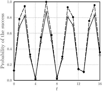
Figure 1: $P_{\mathrm{suc}}(t)$ as a function of integer $t$ is shown by solid line for $\alpha=0.72$ and by dashed line for $\alpha=0$. Both the lines are related to the case $N=16$ and $M=2$.

For the uniform initial distribution, the rescaled initial amplitudes are written as

$$k_{x}^{\,\prime}(0)=\frac{1}{\sqrt{1\pm\alpha}}\ ,\qquad\ell_{y}^{\,\prime}(0)=\frac{1}{\sqrt{1\pm\alpha}}\ .$$

By substituting, the initial averaged amplitudes then read as

$$\widetilde{k}^{\,\prime}(0)=\widetilde{\ell}^{\,\prime}(0)=\frac{\sqrt{1+\alpha}+\sqrt{1-\alpha}}{2}\ .$$

Unlike the above balanced cases, the initial differences take non-zero values, namely

$$\Delta{k}_{x}^{\,\prime}=\Delta\ell_{y}^{\,\prime}=\frac{1}{\sqrt{1\pm\alpha}}-\frac{\sqrt{1+\alpha}+\sqrt{1-\alpha}}{2}\ .$$ (65)

Since $\widetilde{k}^{\,\prime}(0)=\widetilde{\ell}^{\,\prime}(0)$, we can obtain the coefficients $\xi_{1}$, $\xi_{2}$, $\xi_{3}$, $\xi_{4}$ as follows. The expressions (42) and (43) should all be multiplied by the factor $\bigl{(}\sqrt{1+\alpha}+\sqrt{1-\alpha}\,\bigr{)}/\sqrt{2}$. Hence, the averaged amplitudes become

$$\widetilde{k}^{\,\prime}(t) =\frac{\sqrt{1+\alpha}+\sqrt{1-\alpha}}{2}\ \frac{\sin\bigl{[}\omega(t+1/2)\bigr{]}}{\sin\omega/2}\ ,$$

$$\widetilde{\ell}^{\,\prime}(t) =\frac{\sqrt{1+\alpha}+\sqrt{1-\alpha}}{2}\ \frac{\cos\bigl{[}\omega(t+1/2)\bigr{]}}{\cos\omega/2}\ .$$

Hence, we obtain the amplitudes of marked and unmarked states in the form

$$k_{x}(t) =\sqrt{\frac{1\pm\alpha}{N}}\left(\widetilde{k}^{\,\prime}(t)+\frac{1}{\sqrt{1\pm\alpha}}-\frac{\sqrt{1+\alpha}+\sqrt{1-\alpha}}{2}\,\right),$$ (66)

$$\ell_{y}(t) =\sqrt{\frac{1\pm\alpha}{N}}\left(\widetilde{\ell}^{\,\prime}(t)+\frac{(-1)^{t}}{\sqrt{1\pm\alpha}}-\frac{\sqrt{1+\alpha}+\sqrt{1-\alpha}}{2\,(-1)^{t}}\,\right).$$ (67)

For each of the lines (66) and (67), we have the sign plus and the sign minus exactly for one half of the amplitudes. By calculations, the desired probabilities are finally expressed as follows. For $\varepsilon=\pm$, we put the quantities

$$P^{(\varepsilon)}(t) =\frac{1}{2}\left[\,\sin\frac{\omega}{2}+\bigl{(}1+\varepsilon\alpha+\sqrt{1-\alpha^{2}}\,\bigr{)}\sin\frac{\omega{t}}{2}\,\cos\frac{\omega(t+1)}{2}\,\right]^{2},$$ (68)

$$Q^{(\varepsilon)}(t) =\frac{1}{2}\left[\,\cos\frac{\omega}{2}-\bigl{(}1+\varepsilon\alpha+\sqrt{1-\alpha^{2}}\,\bigr{)}\sin\frac{\omega{t}}{2}\,\sin\frac{\omega(t+1)}{2}\,\right]^{2},$$ (69)

$$Q^{(\varepsilon)}(t) =\frac{1}{2}\left[\,\cos\frac{\omega}{2}-\bigl{(}1+\varepsilon\alpha+\sqrt{1-\alpha^{2}}\,\bigr{)}\cos\frac{\omega{t}}{2}\,\cos\frac{\omega(t+1)}{2}\,\right]^{2},$$ (70)

where (69) stands for even $t$ and (70) stands for odd $t$. In terms of these quantities, the probabilities of interest are finally expressed as

$$P_{\mathrm{suc}}(t)=P^{(+)}(t)+P^{(-)}(t)\,,\qquad 1-P_{\mathrm{suc}}(t)=Q^{(+)}(t)+Q^{(-)}(t)\,.$$ (71)

An algorithm rate is characterized by the two parameters $\omega$ and $\alpha$. The former corresponds to the original version, whereas the latter reflects the role of prior knowledge. Further, the relative entropy of coherence is represented as

$$C_{1}\bigl{(}|g(t)\rangle\bigr{)}=\sum_{\varepsilon=\pm}P^{(\varepsilon)}(t)\,\ln\biggl{(}\frac{M/2}{P^{(\varepsilon)}(t)}\biggr{)}+\sum_{\varepsilon=\pm}Q^{(\varepsilon)}(t)\,\ln\biggl{(}\frac{(N-M)/2}{Q^{(\varepsilon)}(t)}\biggr{)}\,.$$ (72)

Since the action of (18) is not balanced, the relation between $C_{1}\bigl{(}|g(t)\rangle\bigr{)}$ and $P_{\mathrm{suc}}(t)$ does not follow (52). Due to an inconsistency in amplitude amplification, coherence reducing is not used in the most efficient way. A similar picture occurs with inconsistent prior knowledge in the initial distribution. We refrain from presenting the details here.

To illustrate the above conclusions, we now visualize $C_{1}\bigl{(}|g(t)\rangle\bigr{)}$ versus $t$ for a some simple choice of parameters. We also present both the bounds of the two-sided estimation

$$\max\bigl{\{}h_{1}\bigl{(}P_{\mathrm{suc}}(t)\bigr{)},-\ln\Omega(t)\bigr{\}}\leq{C}_{1}\bigl{(}|g(t)\rangle\bigr{)}\,,$$ (73)

$$C_{1}\bigl{(}|g(t)\rangle\bigr{)}\leq P_{\mathrm{suc}}(t)\,\ln\!\left(\frac{M}{P_{\mathrm{suc}}(t)}\right)+\bigl{(}1-P_{\mathrm{suc}}(t)\bigr{)}\ln\!\left(\frac{N-M}{1-P_{\mathrm{suc}}(t)}\right).$$ (74)

With changes of $t$, the condition $\arg\bigl{(}\max{p}(x)\bigr{)}\in{\mathcal{M}}$ is violated from time to time.

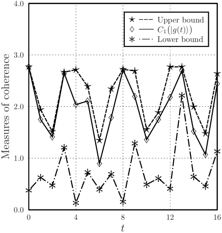
Figure 2: The relative entropy of coherence $C_{1}\bigl{(}|g(t)\rangle\bigr{)}$ and bounds on it as functions of $t$ for the case $N=16$, $M=2$, and $\alpha=0.72$.

In Figs. 1 and 2, we visualize the results for the case $N=16$, $M=2$, and $\alpha=0.72$. In Fig. 1, the success probability is shown as a function of $t$. For comparison, the success probability is also given for $\alpha=0$. It seems that small variations of $\alpha$ do not alter essentially the optimal measurement time. We also observe that an inconsistency of amplitudes of the state $|\eta\rangle$ leads to some decreasing of the probability peaks. On the other hand, reaching one or another peak requires the same number of iteration as in the original formulation. We also observe that the trade-off line between $C_{1}\bigl{(}|g(t)\rangle\bigr{)}$ and the success probability does not follow the upper bound exactly. Dealing with marked and unmarked states inconsistently, this form of amplitude amplification cannot always use coherence changes in the most efficient way in the sense of impact on the success probability. Using Fig. 2, we can also estimate a quality of bounds in the two-sided estimate (28). As explicit general bounds, they seem to be sufficiently useful.

IV.4 An example of mixed states in original Grover’s formulation

In this section, we briefly exemplified the statements of Propositions 1 and 2 in application to mixed states. We restrict a consideration to impure states of the form

$$\boldsymbol{\varrho}(\vartheta)=(1-\vartheta)|\nu\rangle\langle\nu|+\vartheta|\mu\rangle\langle\mu|\,,$$ (75)

where $\vartheta\in[0;1]$ and the normalized pure states $|\nu\rangle$ and $|\mu\rangle$ are defined as

$$|\nu\rangle:=\frac{1}{\sqrt{N-M}}\sum_{y\in{\mathcal{M}}^{{\mathtt{C}}}}|y\rangle\,,\qquad|\mu\rangle:=\frac{1}{\sqrt{M}}\sum_{x\in{\mathcal{M}}}|x\rangle\,.$$ (76)

For such states, we can express results analytically. First of all, we observe the equality ${\mathsf{G}}_{0}\,\boldsymbol{\varrho}(\vartheta)\,{\mathsf{G}}_{0}=\boldsymbol{\varrho}(\vartheta)$. In other words, states of the form (75) are not changed during the Grover search. It is also obvious that $P_{\mathrm{suc}}(t)=\vartheta$. Doing some calculations, we further obtain the result

$$\underset{\boldsymbol{\delta}\in{\mathcal{I}}}{\max}\,\bigl{\|}\sqrt{\boldsymbol{\varrho}(\vartheta)}\,\sqrt{\boldsymbol{\delta}}\,\bigr{\|}_{1}=\sqrt{\frac{\vartheta}{M}+\frac{1-\vartheta}{N-M}}\ ,\qquad C_{\mathrm{g}}\bigl{(}\boldsymbol{\varrho}(\vartheta)\bigr{)}=1-\frac{\vartheta}{M}-\frac{1-\vartheta}{N-M}\ .$$ (77)

Comparing the latter with (22), we see the following. The left-hand side of (22) vanishes, whereas the right-hand side excesses $C_{\mathrm{g}}\bigl{(}\boldsymbol{\varrho}(\vartheta)\bigr{)}$ by the term $(1-\vartheta)\big{/}(N-M)$. It is a typical case, when the number of marked states is very small in comparison with the total search space. In this situation, the upper bound of Proposition 1 becomes almost tight. It is also obvious that $S_{1}\bigl{(}\boldsymbol{\varrho}(\vartheta)\bigr{)}=h_{1}(P_{\mathrm{suc}})$. Thus, the left-hand side of the relation (28) vanishes with states of the form (75). Although we see some anti-correlation between the coherence measures and the success probability with respect to varying $\vartheta$, for each concrete $\boldsymbol{\varrho}(\vartheta)$ the success probability is constant. The latter may change during amplitude amplification with generalized blocks that deal with marked and unmarked states consistently. Thus, quantum coherence alone is insufficient as a resource for the original Grover algorithm.

V Conclusions

We have addressed the role of dealing with quantum coherence in amplitude amplification processes. General trade-off relations between quantum coherence and the success probability were derived. It seems that the geometric coherence and the relative entropy of coherence are more convenient quantifiers in this context. In comparison with the geometric coherence, the relative entropy of coherence is recognized as more sensitive. We obtained inequalities that can be used for estimating the relative entropy of coherence. Basic conclusions are supported by explicit consideration of several model scenarios of amplitude amplification. Coherence changes can be used in the most efficient way only when marked and unmarked states are dealt with consistently. In other words, the computing process does not distinguish between the marked states as well as between the unmarked ones. Then any coherence decreasing will amplify the success probability as much as possible. Otherwise, there is a difference between concrete marked states and, maybe, unmarked states. In this unbalanced case, the relative entropy of coherence does not reach always its maximal value approved by the two-sided estimate for the given value of the success probability. Our results evidence that even tight trade-offs between coherence and the success probability do not imply always an enhancement of amplitude amplification.

Appendix A Results of analyzing the recursion equations

In this section, we briefly recall some formulas for the amplitudes in a generalized version of Grover’s search with arbitrary initial distribution biham2000 . The solution is expressed in terms of rescaled amplitudes

$$k_{x}^{\,\prime}(t)=\eta_{x}^{-1}k_{x}(t)\,,\qquad\ell_{y}^{\,\prime}(t)=\eta_{y}^{-1}\ell_{y}(t)\,.$$ (78)

where the coefficients $\eta_{z}=\langle{z}|\eta\rangle$ are assumed to be nonzero for all $z\in{\mathcal{M}}\cup{\mathcal{M}}^{{\mathtt{C}}}$. Introducing the weights

$$W_{k}=\sum_{x\in{\mathcal{M}}}|\eta_{x}|^{2}\,,\qquad W_{\ell}=\sum_{y\in{\mathcal{M}}^{{\mathtt{C}}}}|\eta_{y}|^{2}\,,$$ (79)

so that $W_{k}+W_{\ell}=\langle\eta|\eta\rangle=1$, the authors of biham2000 defined weighted averages of rescaled amplitudes

$$\widetilde{k}^{\,\prime}(t) =\frac{1}{W_{k}}\sum_{x\in{\mathcal{M}}}|\eta_{x}|^{2}\,k_{x}^{\,\prime}(t)\,,$$ (80)

$$\widetilde{\ell}^{\,\prime}(t) =\frac{1}{W_{\ell}}\sum_{y\in{\mathcal{M}}^{{\mathtt{C}}}}|\eta_{y}|^{2}\,\ell_{y}^{\,\prime}(t)\,.$$ (81)

Then the recursion equations can be converted into a single matrix equation. This matrix equation has been solved by diagonalizing some $2\times 2$ matrix biham2000 . The eigenvalues of this matrix are expressed as

$$\lambda_{\pm}=e^{{\mathtt{i}}\omega_{\pm}}\,,\qquad\omega_{\pm}=\pi+\frac{\beta+\gamma}{2}\pm\omega\,,$$ (82)

where the parameter $\omega$ obeys $0\leq\omega\leq\pi$ and

$$\cos\omega=W_{k}\,\cos\frac{\beta+\gamma}{2}+W_{\ell}\,\cos\frac{\beta-\gamma}{2}\ .$$ (83)

Under assumptions $W_{k}\neq 0$ and $W_{\ell}\neq 0$ together with $\gamma\in(0;2\pi)$, the matrix of interest is certainly diagonalizable. The averaged amplitudes are finally expressed as

$$\widetilde{k}^{\,\prime}(t) =\xi_{1}e^{{\mathtt{i}}\omega_{+}t}-\xi_{2}e^{{\mathtt{i}}\omega_{-}t}\,,$$ (84)

$$\widetilde{\ell}^{\,\prime}(t) =\xi_{3}e^{{\mathtt{i}}\omega_{+}t}-\xi_{4}e^{{\mathtt{i}}\omega_{-}t}\,,$$ (85)

where the coefficients are found as $a=\bigl{(}1-e^{{\mathtt{i}}\beta}\bigr{)}\,e^{{\mathtt{i}}\gamma}W_{k}-e^{{\mathtt{i}}\gamma}$, $b=\bigl{(}1-e^{{\mathtt{i}}\beta}\bigr{)}W_{\ell}$ and

$$\xi_{1} =\frac{(\lambda_{-}-a)\widetilde{k}^{\,\prime}(0)-b\,\widetilde{\ell}^{\,\prime}(0)}{\lambda_{-}-\lambda_{+}}\ , \xi_{2} =\frac{(\lambda_{+}-a)\widetilde{k}^{\,\prime}(0)-b\,\widetilde{\ell}^{\,\prime}(0)}{\lambda_{-}-\lambda_{+}}\ ,$$

$$\xi_{3} =\frac{\lambda_{+}-a}{b}\>\xi_{1}\ , \xi_{4} =\frac{\lambda_{-}-a}{b}\>\xi_{2}\ .$$ (86)

Introducing the initial differences

$$\Delta{k}_{x}^{\,\prime} =k_{x}^{\,\prime}(0)-\widetilde{k}^{\,\prime}(0)\,,$$ (87)

$$\Delta\ell_{y}^{\,\prime} =\ell_{y}^{\,\prime}(0)-\widetilde{\ell}^{\,\prime}(0)\,,$$ (88)

the solution is completed by the formulas biham2000

$$k_{x}^{\,\prime}(t) =\widetilde{k}^{\,\prime}(t)+(-1)^{t}e^{{\mathtt{i}}\gamma{t}}\Delta{k}_{x}^{\,\prime}\,,$$ (89)

$$\ell_{y}^{\,\prime}(t) =\widetilde{\ell}^{\,\prime}(t)+(-1)^{t}\Delta\ell_{y}^{\,\prime}\,.$$ (90)

References

- (1) Grover, L.K.: Quantum mechanics helps in searching for a needle in a haystack. Phys. Rev. Lett. 79, 325–328 (1997)
- (2) Grover, L.K.: Quantum computers can search arbitrarily large databases by a single query. Phys. Rev. Lett. 79, 4709–4712 (1997)
- (3) Grover, L.K.: Quantum computers can search rapidly by using almost any transformation. Phys. Rev. Lett. 80, 4329–4332 (1998)
- (4) Shor, P.W.: Polynomial-time algorithms for prime factorization and discrete logarithms on a quantum computer. SIAM J. Comput. 26, 1484–1509 (1997)
- (5) Haase, D., Maier, H.: Quantum algorithms for number fields. Fortschr. Phys. 54, 866–881 (2006)
- (6) Hallgren, S.: Polynomial-time quantum algorithms for Pell’s equation and the principal ideal problem. J. ACM 54, 4 (2007)
- (7) Childs, A.M., van Dam, W.: Quantum algorithms for algebraic problems. Rev. Mod. Phys. 82, 1–52 (2010)
- (8) Lomonaco, S.J., Kauffman, L.H.: Is Grover’s algorithm a quantum hidden subgroup algorithm? Quantum Inf. Process. 6, 461–476 (2007)
- (9) Bennett, C.H., Bernstein, E., Brassard, G., Vazirani, U.: Strengths and weaknesses of quantum computing. SIAM J. Comput. 26, 1510–1523 (1997)
- (10) Zalka, C.: Grover’s quantum searching algorithm is optimal. Phys. Rev. A 60, 2746–2751 (1999)
- (11) Patel, A.D., Grover, L.K.: Quantum search. In: Kao, M.-Y. (ed.) Encyclopedia of Algorithms, pp. 1707–1716. Springer, New York (2016)
- (12) Biham, E., Biham, O., Biron, D., Grassl, M., Lidar, D.A.: Grover’s quantum search algorithm for an arbitrary initial amplitude distribution. Phys. Rev. A 60, 2742–2745 (1999)
- (13) Biham, E., Biham, O., Biron, D., Grassl, M., Lidar, D.A., Shapira, D.: Analysis of generalized Grover quantum search algorithms using recursion equations. Phys. Rev. A 63, 012310 (2000)
- (14) Biham, E., Kenigsberg, D.: Grover’s quantum search algorithm for an arbitrary initial mixed state. Phys. Rev. A 66, 062301 (2002)
- (15) Deutsch, D.: Quantum theory, the Church–Turing principle and the universal quantum computer. Proc. R. Soc. Lond. A 400, 97–117 (1985)
- (16) Braunstein, S.L., Pati, A.K.: Speed-up and entanglement in quantum searching. Quantum Inf. Comput. 2, 399–409 (2002)
- (17) Jozsa, R., Linden, N.: On the role of entanglement in quantum-computational speed-up. Proc. R. Soc. Lond. A 459, 2011–2032 (2003)
- (18) Baumgratz, T., Cramer, M., Plenio, M.B.: Quantifying coherence. Phys. Rev. Lett. 113, 140401 (2014)
- (19) Adesso, G., Bromley, T.R., Cianciaruso, M.: Measures and applications of quantum correlations. J. Phys. A: Math. Theor. 49, 473001 (2016)
- (20) Streltsov, A., Adesso, G., Plenio, M.B.: Quantum coherence as a resource. Rev. Mod. Phys. 89, 041003 (2017)
- (21) Hu, M.-L., Hu, X., Peng, Y., Zhang, Y.-R., Fan, H.: Quantum coherence and quantum correlations. E-print arXiv:1703.01852 [quant-ph] (2017)
- (22) Hillery, M.: Coherence as a resource in decision problems: The Deutsch-Jozsa algorithm and a variation. Phys. Rev. A 93, 012111 (2016)
- (23) Shi, H.-L., Liu, S.-Y., Wang, X.-H., Yang, W.-L., Yang, Z.-Y., Fan, H.: Coherence depletion in the Grover quantum search algorithm. Phys. Rev. A 95, 032307 (2017)
- (24) Anand, N., Pati, A.K.: Coherence and entanglement monogamy in the discrete analogue of analog Grover search. E-print arXiv:1611.04542 [quant-ph] (2016)
- (25) Farhi, E., Gutmann, S.: Analog analogue of a digital quantum computation. Phys. Rev. A 57, 2403–2406 (1998)
- (26) Nielsen, M.A., Chuang, I.L.: Quantum Computation and Quantum Information. Cambridge University Press, Cambridge (2000)
- (27) Watrous, J.: The Theory of Quantum Information. Cambridge University Press, Cambridge (2018)
- (28) Vedral, V.: The role of relative entropy in quantum information theory. Rev. Mod. Phys. 74, 197–234 (2002)
- (29) Singh, U., Pati, A.K., Bera, M.N.: Uncertainty relations for quantum coherence. Mathematics 4, 47 (2016)
- (30) Peng, Y., Zhang, Y.-R., Fan, Z.-Y., Liu, S., Fan, H.: Complementary relation of quantum coherence and quantum correlations in multiple measurements. E-print arXiv:1608.07950 [quant-ph] (2016)
- (31) Rastegin, A.E.: Uncertainty relations for quantum coherence with respect to mutually unbiased bases. Front. Phys. 13, 130304 (2018)
- (32) Rastegin, A.E.: Quantum coherence quantifiers based on the Tsallis relative entropies. Phys. Rev. A 93, 032136 (2016)
- (33) Shao, L.-H., Li, Y., Luo, Y., Xi, Z.: Quantum coherence quantifiers based on the Rényi -relative entropy. Commun. Theor. Phys. 67, 631–636 (2017)
- (34) Streltsov, A., Kampermann, H., Wölk, S., Gessner, M., Bruß, D.: Maximal coherence and the resource theory of purity. New J. Phys. 20, 053058 (2018)
- (35) Cheng, S., Hall, M.J.W.: Complementarity relations for quantum coherence. Phys. Rev. A 92, 042101 (2015)
- (36) Yuan, X., Bai, G., Peng, T., Ma, X.: Quantum uncertainty relation using coherence. Phys. Rev. A 96, 032313 (2017)
- (37) Hu, M.-L., Fan, H.: Evolution equation for quantum coherence. Sci. Rep. 6, 29260 (2016)
- (38) Shao, L.-H., Xi, Z., Fan, H., Li, Y.: Fidelity and trace-norm distances for quantifying coherence. Phys. Rev. A 91, 042120 (2015)
- (39) Rana, S., Parashar, P., Lewenstein, M.: Trace-distance measure of coherence. Phys. Rev. A 93, 012110 (2016)
- (40) Uhlmann, A: The ’transition probability’ in the state space of a *-algebra. Rep. Math. Phys. 9, 273–279 (1976)
- (41) Jozsa, R.: Fidelity for mixed quantum states. J. Mod. Optics 41, 2315–2323 (1994)
- (42) H.-J. Zhang, B. Chen, M. Li, S.-M. Fei and G.-L. Long, Estimation on geometric measure of quantum coherence. Commun. Theor. Phys. 67, 166– (2017)
- (43) Bera, M.N., Qureshi, T., Siddiqui, M.A., Pati, A.K.: Duality of quantum coherence and path distinguishability. Phys. Rev. A 92, 012118 (2015)
- (44) Bagan, E., Bergou, J.A., Cottrell, S.S., Hillery, M.: Relations between coherence and path information. Phys. Rev. Lett. 116, 160406 (2016)
- (45) Qureshi, T., Siddiqui, M.A.: Wave-particle duality in -path interference. Ann. Phys. 385, 598–604 (2017)
- (46) Hu, M.-L., Fan, H.: Relative quantum coherence, incompatibility and quantum correlations of states. Phys. Rev. A 95, 052106 (2017)
- (47) Ambainis, A., Schulman, L.J., Vazirani, U.: Computing with highly mixed states. J. ACM 53, 507–531 (2006)
- (48) Popescu, P., Sluşanschi, E.-I., Iancu, V., Pop, F.: A new upper bound for Shannon entropy. A novel approach in modeling of Big Data applications. Concurrency Computat.: Pract. Exper. 28, 351–359 (2016)