Surfing the edge: using feedback control to find nonlinear solutions

Abstract

Many transitional wall-bounded shear flows are characterised by the coexistence in state-space of laminar and turbulent regimes. Probing the edge boundary between the two attractors has led in the last decade to the numerical discovery of new (unstable) solutions to the incompressible Navier–Stokes equations. However, the iterative bisection method used to compute edge states can become prohibitively costly for large systems. Here we suggest a simple feedback control strategy to stabilise edge states, hence accelerating their numerical identification by several orders of magnitude. The method is illustrated for several configurations of cylindrical pipe flow. Travelling waves solutions are identified as edge states, and can be isolated rapidly in only one short numerical run. A new branch of solutions is also identified. When the edge state is a periodic orbit or chaotic state, the feedback control does not converge precisely to solutions of the uncontrolled system, but nevertheless brings the dynamics very close to the original edge manifold in a single run. We discuss the opportunities offered by the speed and simplicity of this new method to probe the structure of both state space and parameter space.

1 Introduction

In the recent years, there has been increasing evidence for the dynamical importance of exact unstable solutions, such as travelling waves or periodic orbits, for weakly turbulent flows (Kawahara et al., 2012; Chandler & Kerswell, 2013; Cvitanović, 2013; Willis et al., 2016). This is best understood so far for the case of subcritical wall-bounded shear flows, where the base flow is linearly stable at flow rates where turbulence is also sustained. These unstable solutions are the only non-trivial solutions, and are all disconnected from the trivial laminar solution (Eckhardt et al., 2007).

Most solutions discovered so far appear in saddle-node bifurcations and hence arise in pairs. The solution on the lower energy branch often belongs to the laminar-turbulent separatrix, “the edge”, which separates initial conditions that lead to relaminarisation from those that experience transition to turbulence (Itano & Toh, 2001; Skufca et al., 2006). The attractor within the edge separatrix is labelled the “edge state”. When a solution located on the edge has only one real unstable eigenvalue, it acts as an attractor within the edge. There may be more than one edge state for a given system. Upper branch solutions are thought to be either embedded in the turbulent attractor, or, together with the lower branch solution, bracket the turbulent dynamics (Gibson et al., 2008).

Knowledge of an invariant solution within the edge has become the first step of a common strategy to unfold the whole bifurcation diagram of the system (Kreilos & Eckhardt, 2012; Avila et al., 2013; Ritter et al., 2016), but identification of exact coherent states remains a demanding task. In the absence of a well-understood sequence of bifurcations from the base flow, i.e. when all classical continuation methods fail (Tuckerman & Barkley, 2000), several strategies have been employed to find such solutions. The size of the systems under study, usually with $10^{4}$ to $10^{9}$ degrees of freedom, requires specialised iterative strategies, which in particular avoid any operation involving the storage of full matrices. A perhaps more challenging issue is that a good initial guess for the identification is usually unavailable. During the 1990s and early 2000s, the main strategy used to bypass this issue was homotopy (see e.g. Kerswell (2005)). This relies on an efficient root finder, typically a Newton–Raphson solver coupled to an arc-length continuation algorithm. This method may track the solutions in parameter space, but does not help to identify unconnected branches. To apply this method, a companion problem featuring a linear instability of the base flow must first be identified. Once a bifurcated solution is found, it is continued nonlinearly to a solution of the original problem. Success requires very good intuition for suitable homotopies that might work, plus involves the complexity of solving for the multiple systems. It is also unclear how continued solutions participate in the dynamics.

Later, bisection methods, which make use of timesteppers, began to gain popularity: the amplitude of an arbitrary perturbation to the base flow is rescaled repeatedly, until a trajectory is found which for a sufficiently long time stays away from both the laminar and the turbulent state (Itano & Toh, 2001; Skufca et al., 2006; Schneider et al., 2007). Such a trajectory is usually chaotic, but with some luck, if there exists a regular solution with only one unstable eigendirection, there is hope that the bisection algorithm will converge to it (Schneider et al., 2008). Imposing discrete symmetries to the dynamics often reduces the number of unstable eigendirections of the ECS contained in the associated subspace (Duguet et al., 2008b). As a result the likelihood of identifying symmetry-invariant solutions is increased, but their relevance to the non-symmetric dynamics is uncertain. In the more general case where the edge trajectory is chaotic, recurrence analysis can sometimes identify an approach to a simple state, which can be converged using a good Newton solver, possibly enhanced by some globalisation method (Viswanath, 2007; Duguet et al., 2008a). The main drawbacks of bisection methods are the hazardous chances of success, the difficulty to converge interesting recurrent parts of the dynamics using Newton methods, and more importantly their cost. Indeed one bisection requires $2^{n}$ individual runs until machine precision $\varepsilon_{M}$ is reached at $n^{th}$ iteration, i.e. $n\sim-\log_{2}(\varepsilon_{M})$, at which point the process needs to be restarted $M$ times while no simple edge state has been reached. The total cost is hence of $Mn\geq$ 100 runs at least, with the runs getting longer as the accuracy improves. For instance, in Khapko et al. (2016), each bisection required a total of $Mn\approx$ 400 runs, which corresponds to $O(10^{6}-10^{7})$ CPU hours. This high cost makes parametric studies infeasible in practice. Other numerical methods have been suggested as alternatives to the bisection-rootfinder combination, e.g. iterative adjoint optimisation methods (Farazmand, 2016; Olvera & Kerswell, 2017) though they involve significant mathematical and computational complexity. In summary, it is always desirable to find simpler and less expensive alternative methods.

In the present paper we demonstrate how unstable edge states can be found numerically, by introducing into the original system a “control” term that counteracts the edge instability and is able to stabilise unstable states without altering them significantly. This enables the system to dynamically approach the edge state in a single simulation of the controlled system. A key property of a control for this purpose is that it should influence only the stability, not the structure of the a priori unknown target, i.e. the control should act as non-invasively as possible. At the same time, it should efficiently force a large set of initial conditions towards the states of interest. Using control as a tool to numerically find and analyse unstable objects in a complex dynamical system has already been successfully applied to a variety of problems. A classical example is the time-delayed feedback control (Pyragas, 1992) able to stabilise certain periodic orbits provided their period is known. Another example is Selective Frequency Damping, which, by filtering all non-zero temporal frequencies, may stabilise steady state solutions (Åkervik et al., 2006). In the latter case, however, the steady solutions must not possess unstable non-oscillatory eigenvalues (Vyazmina, 2010), which is frequently the case for edge solutions in subcritical shear flows. Note that none of these methods is designed to target the edge manifold.

In this article we propose a remarkably simple linear feedback control able to constrain the dynamics to the edge manifold, and to stabilise invariant solutions that are stable within the edge. This scheme has recently been applied to track unstable chimera states in systems of non-locally coupled phase oscillators (Sieber et al., 2014; Wolfrum et al., 2015). In an interesting analogy to shear flows, in systems of coupled oscillators “chimera” are metastable chaotic states that coexist with a fully synchronized (”laminar”) state (Panaggio & Abrams, 2015). The chimera also appear in a saddle-node bifurcation, and the corresponding unstable lower branch also acts as an edge state separating the synchronous from the chimera regime. In the current fluid context, we first need to restrict the dynamics to the low-energy levels characteristic of the edge manifold. So far, the bisection method has revealed that the dynamics on the edge manifold is relatively low-dimensional, especially compared to turbulent flow at equivalent parameters values (Duguet et al., 2008b). We wish to take advantage of this property to extract invariant solutions from the controlled flow, in the same way that solutions have been extracted from edge bisections. Our aim here, however, is to achieve this in a single simulation, rather than via the more expensive bisection approach.

In the following section we describe the feedback control, then in §3 we present the numerical set-up. In §4 we apply the control scheme to several different pipe flow cases, first in a restricted domain and then in an extended domain allowing for axial localisation. Finally possible applications for the methods are discussed in the concluding §5.

2 Stabilisation of lower branch equilibria by feedback control

In its most simple form, the control scheme makes a system parameter $\mu$ state-dependent by imposing a linear relation between the parameter and an observable $A(t)$

$$\mu(t)=\mu_{0}+\kappa(A_{0}-A(t))\,.$$ (1)

(For the shear flow problems we will identify $\mu$ with $Re$ and $A$ with a component of the perturbation energy.) How such a proportional control can be used to stabilize the unstable part of a folded branch can be explained by applying it to the normal form for a saddle-node bifurcation,

$$\dot{x}(t)=\mu-x^{2}(t).$$ (2)

where equilibria lie on the parabola $\mu=x^{2}$. Inserting the constraint (1) in to (2) and choosing the simplest possible observable $A\equiv x$, we arrive at the equation

$$\dot{x}=f(x,\kappa,\mu_{0},x_{0}):=\mu_{0}+\kappa(x_{0}-x)-x^{2}.$$ (3)

Geometrically, the resulting dynamics can be understood by considering its representation in the $(\mu,x)$ plane. For $\kappa=0$ we have the uncontrolled system (2), where for a fixed choice of the parameter the dynamics are constrained to a vertical line $\mu=\mu_{0}$. in the $(\mu,x)$ plane. Equilibria are located at the intersections of the vertical line with the parabola, $x=\pm\sqrt{\mu}$. According to equation (2), $x$ increases with time in the region enclosed by the parabola, for $x^{2}<\mu$, while it decreases outside of this region. Hence, we conclude that for the uncontrolled system the equilibria on the upper branch, $x=+\sqrt{\mu}$, of the parabola are dynamically stable, while those on the lower branch, $x=-\sqrt{\mu}$, are unstable.

Restricting now the dynamics to a slanted straight line, as imposed by (1) with $\kappa>0$, we obtain the controlled system (3), which has equilibria

$$x_{\pm}=\frac{1}{2}\left(-\kappa\pm\sqrt{\kappa^{2}+4(\mu_{0}+\kappa x_{0})}\right),$$ (4)

provided that

$$\kappa^{2}+4(\mu_{0}+\kappa x_{0})=(\kappa+2x_{0})^{2}+4(\mu_{0}-x_{0}^{2})>0.$$ (5)

Note that the equilibria (4) coincide with the equilibria of the uncontrolled system (2) for the particular choice $\mu=\mu_{0}+\kappa(x_{0}-x_{\pm})$. The controlled system has derivative

$$\partial_{x}f(x_{\pm},\kappa,\mu_{0},x_{0})=-\kappa-2x_{\pm}=\mp\sqrt{\kappa^{2}+4(\mu_{0}+\kappa x_{0})}.$$

Thus the upper intersection $x_{+}$ of the controlled system is stable, while $x_{-}$ is unstable. In particular, whilst the lower branch $x=-\sqrt{\mu}$ is unstable for $\kappa=0$, it is possible to choose a slanted straight line such that both intersections $x_{\pm}$ meet the parabola on the lower branch. The upper intersection $x_{+}$ is now a stablised equilibrium on the lower branch. Further, by varying the control gain $\kappa$, we can now sweep the straight line about the pivot point $(\mu_{0},x_{0})$ to track the branch of stable equilibria of the controlled system. This is possible until the straight line becomes tangential to the parabola, when the $x_{\pm}$ disappear via a saddle-node bifurcation for $|\kappa+2x_{0}|>2\sqrt{x_{0}^{2}-\mu_{0}}.$

The proportional control (1) can be applied in the same way to a system with more complicated dynamics, shown schematically in figure 1, provided that it contains a saddle-node bifurcation. Such a folded branch of flow invariant manifolds generically develops a single transversal direction of instability, similar to the example above. Using an observable that varies along the fold, we can apply the control. Whenever we obtain a controlled state with constant observable, it will exactly coincide with a dynamical state of the uncontrolled system with fixed parameter related to the constant observable by (1). Only the stability properties may be affected by the control, i.e. the control is non-invasive for such states. Controlled trajectories with periodic or chaotic fluctuations in $A(t)$ may still show good quantitative and qualitative agreement with an uncontrolled trajectory for a parameter value close to the time-average $\langle\mu\rangle_{t}$. The control may be described as non-invasive on average (Sieber et al., 2014). In this way, in the shear flow problems it will be possible to obtain periodic orbits to be used as initial states for a corresponding Newton solver. Also, by sweeping the control gain dynamically from a known stable dynamical regime of the uncontrolled system, the controlled system may yield access to qualitatively different dynamical regimes along the lower branch, i.e. the edge.

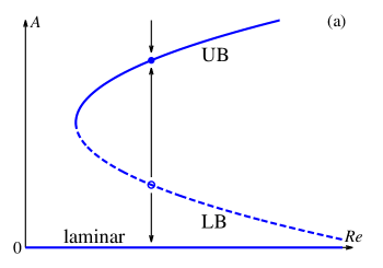
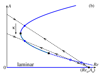
Figure 1: Sketch in an $(A,Re)$ representation of the stability of the uncontrolled (a) and controlled system using the feedback control method (b) based on the constraint (1) corresponding to the dashed slanted line. The labels ‘UB’ and ‘LB’ refer to the stable upper and unstable lower branch in the uncontrolled system, respectively. In figure 1b the dynamics is restricted to a dashed slanted line. Rotating the line about a pivot point, fixed points on LB are stabilised and can be tracked dynamically.

3 Numerical methodology

3.1 Direct numerical simulation of pipe flow

We consider here the case of cylindrical pipe flow with a fixed mass flux. The control parameter $\mu$ in Eq. (1) is here the Reynolds number $Re=UD/\nu$, where $U$ is the constant bulk velocity, $D$ the pipe diameter and $\nu$ the kinematic viscosity of the fluid. Using $U$ and $D$ as the scales, the non-dimensional laminar state is characterised by an axial velocity profile ${\bm{u}}_{\mathrm{lam}}(r)=2(1-(2r)^{2}){\bm{e}}_{z}$ for $0\leq r\leq\frac{1}{2}$, driven by a homogeneous pressure gradient $(\partial_{z}p_{lam}){\bm{e}}_{z}$. The full velocity field ${\bm{u}}=(u,v,w)$, which contains the radial, azimuthal and axial components of the velocity, satisfies together with the pressure $p$ the incompressible Navier–Stokes equations at all times :

$${\bm{\nabla}}\cdot{\bm{u}} = 0,$$ (6)

$$\frac{\partial{\bm{u}}}{\partial t}+\left({\bm{u}}\cdot{\bm{\nabla}}\right){\bm{u}} = -{\bm{\nabla}}p+\frac{1}{Re}{\bm{\nabla}}^{2}{\bm{u}}.$$ (7)

The flow satisfies the no-slip velocity conditions at the wall. The code ensures that this condition is satisfied to machine precision via the influence matrix method (Kleiser & Schumann, 1980). We advance (7) in time using the hybrid spectral finite-difference code openpipeflow.org (Willis, 2017). The code employs Fourier expansions $\mathrm{e}^{\mathrm{i}(2\alpha kz+mm_{0}\theta)}$, where $k$ and $m$ are respectively the axial and the azimuthal wavenumbers. This imposes streamwise periodicity with a wavelength $L=\pi/\alpha$ in units $D$. The integer $m_{0}$ indicates the degree of rotational symmetry of the flow field in the azimuthal direction, $m_{0}=2$ refers to a two-fold symmetry while $m_{0}=1$ corresponds to the absence of any discrete rotational symmetry. In some cases we also impose mirror symmetry $Z{\bm{u}}={\bm{u}}$ about the plane $\theta=0$, where

$$Z:(u,v,w,p)(r,\theta,z)\rightarrow(u,-v,w,p)(r,-\theta,z),$$ (8)

and the shift-and-reflect symmetry $S{\bm{u}}={\bm{u}}$, where

$$S:(u,v,w,p)(r,\theta,z)\rightarrow(u,-v,w,p)(r,-\theta,z+L/2).$$ (9)

In subsections (3.1) and (3.2) we consider simulations with $m_{0}=2$ in domains with respectively $\alpha=1.25$ and $0.12566$. With dealiasing, variables are evaluated on grids in $r\times\theta\times z$ of respectively $64\times 48\times 72$ and $64\times 48\times 576$ points. In subsection (3.3), for $m_{0}=1$ and $\alpha=1.25$, the resolution is $64\times 96\times 72$.

3.2 Implementation of the feedback control.

For the Navier–Stokes system (6)–(7), the feedback control (1) is applied by controlling the Reynolds number

$$Re(t)=Re_{0}+\kappa(A_{0}-A(t))$$ (10)

using the scalar observable

$$A(t)=\int_{r_{i}}^{r_{w}}(u^{2}+v^{2})\,r\,\mathrm{d}r\,\mathrm{d}\theta\,\mathrm{d}z\,,$$ (11)

where $r_{w}$=0.5 corresponds to the wall and $r_{i}$ is set to 0.35. This observable $A$, considered only over the near-wall annular region $r_{i}\leq r\leq r_{w}$, is a robust signature of the presence of active coherent structures contributing to the turbulence production. Several other observables were examined, such as energies that include all components of the velocity, integrated over the whole domain, or the energy input related to the average wall drag. No significant difference between those observables was noted in the application of the method, which indicates the robustness of the control approach.

The factor $1/Re$ appears as the coefficient of the viscous term, which is treated implicitly in our timestepping scheme, and the factor is used in the evaluation of time stepping matrices. Now that $Re$ depends on time, rather than recalculating these matrices every time step, we consider the governing equation (7) in the form

$$\frac{\partial{\bm{u}}}{\partial t}-\frac{1}{Re_{r}}{\bm{\nabla}}^{2}{\bm{u}} ~{}=~{} \left(\frac{1}{Re}-\frac{1}{Re_{r}}\right)\,{\bm{\nabla}}^{2}{\bm{u}}-\left({\bm{u}}\cdot{\bm{\nabla}}\right){\bm{u}}-{\bm{\nabla}}p\,,$$ (12)

where $Re_{r}$ is a reference value kept within 1% of $Re(t)$. The diffusion term on the left-hand side of (12) is treated implicitly. The small correction term with coefficient $(1/Re-1/Re_{r})$, along with the rest of the terms on the right-hand side, is treated explicitly. No numerical instability has been observed.

We now explain how to choose the constants $A_{0}$ and $Re_{0}$. $A_{0}$ was chosen to be zero so that $Re(t)\to Re_{0}$ as $A(t)\to 0$, i.e. as the observable approaches zero $Re(t)$ approaches a maximum value. Since at low $Re$ turbulence frequently relaminarises, the value of $Re_{0}$ must be chosen to be sufficiently high to avoid such relaminarisations. It is determined indirectly from the value of $\kappa$ necessary to stabilise turbulence at lower $Re$ and lower amplitudes $A$: For a trial $Re_{0}$ and knowing $(Re,A)$ for a given (uncontrolled) velocity field, from (1) we can estimate a starting value for $\kappa$. Starting controlled simulations with $\kappa$ at two or three times this value, in order to enforce a lower $A(t)$, we then adjusted $Re_{0}$ to avoid relaminaristions. Thereafter, the value $Re_{0}=10^{4}$ was found to be adequate for all further simulations, giving the pivot point $(Re_{0},A_{0})=(10^{4},0)$.

Using a large value of $Re_{0}$ at first sight suggests that spatial resolution issues may arise for large $Re(t)$. In practice, no fully turbulent simulation is run at values of $Re$ as high as $Re_{0}$. Large $Re(t)$ occurs only for small energies $A(t)$, for which the spectral drop-off is more rapid. It has been verified that the drop-off in energy spectra is sufficient that all stabilised states considered in this paper are well resolved.

Finally, we discuss the time-dependence of the control gain $\kappa(t)$. Continuation along the lower-energy branch towards increasing $Re$ requires the slope of the line given by (2) in the $(Re,A)$ plane to decrease, i.e. $\kappa(t)$ must increase with time. Once the energy $A(t)$ has dropped below its level for the uncontrolled system, it becomes more difficult to change $\kappa$ in steps without each step causing an initial wild fluctuation in $Re(t)$, which in turn is likely to cause immediate relaminarisation. This issue is avoided by allowing $\kappa(t)$ to vary smoothly. A simple exponential form for $\kappa(t)$ proved effective

$$\kappa(t)=\kappa_{0}\,\mathrm{e}^{t/T},$$ (13)

where $T$ is a chosen time-scale constant. $T$ is also the expected time-scale for the rate of decrease in the resulting controlled $A(t)$. The approach is quite insensitive to the precise choice of $T$ (example in §4.1). As far as convergence to invariant solutions is concerned, $T$ should be longer than the decay time of the least-damped mode for the stabilised solution of the controlled system. Since this is unknown, $T$ is simply chosen to be long relative to the $O(1-10)$ time scale of the variability observed in energy and disspation time series.

4 Results

4.1 Short periodic pipe with $m_{0}$=2

We present first the results with the feedback control for a short pipe of length $L=2\pi/\alpha$ with $\alpha=1.25$, $m_{0}=2$ and no additional symmetry. This system was considered in (Kerswell & Tutty, 2007), and was shown to possess a lower-branch travelling wave (TW) with only one unstable real eigenvalue. It was later verified in (Duguet et al., 2008b) that bisection in this system could identify a travelling wave as edge state, but further, that bisection could converge to two travelling waves from different families, depending on the initial condition. We describe now how the feedback controller described in the previous section successfully identified and stabilised another travelling wave solution on the edge.

We start from a turbulent snapshot at $Re=2000$, then vary $\kappa(t)$ according to (13) with $T=250$ and $\kappa_{0}=4\times 10^{5}$. As shown in figures 2(a)–(b), the time series of $A(t)$ initially displays erratic fluctuations until $t\approx 300~{}D/U$, where the dynamics appears to be smoother and fluctuations are damped. From $(A,Re)\approx(5\times 10^{-3},1800)$ onwards, the backwards fold in figure 2(a) indicates that the dynamics stays away from the laminar state ($A=0$) and that the whole lower branch is stabilised as far as the simulation is run, up to $Re\approx 3000$ (blue). Halving $T$ (grey), more of the lower branch is quickly reached. Convergence to the same branch is also observed for $T$ doubled (cyan). For the first case, $T=250$, the state $t=375\,D/U$ is used as an initial condition for a controlled simulation with $\dot{\kappa}$ set to zero, i.e. $\kappa$ is held fixed at $\kappa=\kappa_{1}=4\times 10^{5}\times\mathrm{e}^{1.5}$ (green line in figure 2b). The new trajectory converges towards a fixed point, i.e. a travelling wave solution, with constant $A$. The associated velocity field in a cross-section is displayed in figure 3(a). While the symmetry was not imposed, the time integration with the control converged to a solution invariant under $S$, being an S2 state of (Kerswell & Tutty, 2007; Pringle et al., 2009). It was verified using a Newton-solver (Willis et al., 2013) that the corresponding solution is also solution to the original uncontrolled Navier–Stokes equations. The linear stability of the states are compared in their eigenspectrum $\{\sigma\}$, calculated using an Arnoldi algorithm, with and without the control ($\kappa=\kappa_{1}$ and $\kappa=0$, respectively), figure 3(b), where $Re(\sigma)>0$ indicates instability. Whereas the TW is unstable in the uncontrolled system, it is stabilised by the feedback control. Applying the control with $\dot{\kappa}<0$ (here $\kappa(t)=\kappa_{0}\,\mathrm{e}^{-t/T}$) the simulation also remains on the stabilised lower branch, as demonstrated by the green line in figure 2(a). Sweeping along the lower branch in either direction is therefore a very efficient alternative to numerical continuation with a Newton scheme for rapid numerical continuation of the TW solution in this region.

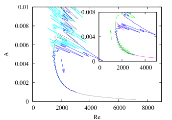
(a) (b)

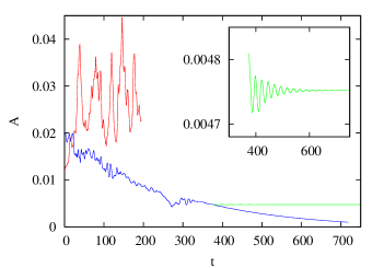
Figure 2: Application of the feedback control for $\alpha=1.25$ and $m_{0}=2$. (a) $(Re,A)$ representation, control with ${\kappa}=\kappa_{0}\exp{(t/T)}$, $T=250$ (blue). Cases with $T$ doubled/halved converge to the same stabilised lower branch (grey/cyan). In the inset, the solution set is compared with results from arc-length continuation (using the Newton method, pink) and continuation in the opposite direction using the control with ${\kappa}=\kappa_{0}\exp{(-t/T)}$ (green). (b) $A(t)$ uncontrolled (red), controlled with time-varying $\kappa(t)$ (blue) and controlled with constant $\kappa$ for the stabilisation of the TW (green) (zoom in inset).

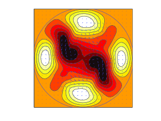
(a) (b)

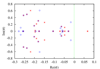
Figure 3: (a) Cross-section of the stabilised TW solution with $\alpha=1.25$ and $m_{0}=2$. Streamwise velocity perturbation in colour (from dark to white) and cross-stream components (vectors). (b) Eigenvalue spectrum for the TW solution with (blue circles) and without control (red crosses).

4.2 Long periodic pipe with $m_{0}$=2

We consider next the case $L=25D$ with $m_{0}=2$ and mirror symmetry $Z$. This system, considered by Avila et al. (2013) and later by Chantry et al. (2014), is known to possess a relative periodic orbit as an edge state, in the form of a weakly modulated travelling wave whose velocity field is axially localised. As in §3.1, a simulation starting from a turbulent state at $Re=1900$ is first used with time-varying $\kappa(t)$ following (13) with $\kappa_{0}=1.62\times 10^{5}$ and $T=400$. Figure 4(a) shows the dynamics in an $(Re,A)$ representation, where for $A\leq 0.03$ a lower branch has been captured by the scheme. At time $t=300\,D/U$ $\kappa$ is held fixed at $\kappa=\kappa_{1}=1.62\times 10^{5}\times\mathrm{e}^{0.75}$. Close-ups on the time series of $A(t)$ and $Re(t)$ show weak periodic modulations around steady values, indicating convergence towards a relative periodic orbit (RPO) (figure 4b). The converged RPO has a time-averaged Reynolds number $\langle Re\rangle_{t}\approx 1450$. A point on this orbit was passed to the Newton solver for the uncontrolled system at $Re=1450$, and converged in one Newton step. The controlled and uncontrolled RPOs do not exactly coincide, but are close. Figure 4(c) show a projection in ($E_{3d},\beta$) (observe the scale and distance from the origin), where $E_{3d}=\int|{\bm{u}}-\langle{\bm{u}}\rangle_{\theta,z}|^{2}\,r\,\mathrm{d}r\,\mathrm{d}\theta\,\mathrm{d}z$ and $1+\beta=\langle\partial_{z}p\rangle/\partial_{z}p_{\mathrm{lam}}$. Their periods are respectively $10.67$ and $10.61$ units $D/U$. Stabilisation is substantiated in the altered Floquet exponents, displayed in figure 4(d). Unlike for the previous short pipe, where the edge state was a travelling wave solution, the controller has achieved convergence to an RPO, which is not precisely a solution to the uncontrolled equations. The control stays approximately non-invasive on average, however, and the isolated solution is close (only a single Newton step was required to go from one solution to the other with a relative error of less than $10^{-6}$). It manages this approach in only one short computation for the large system.

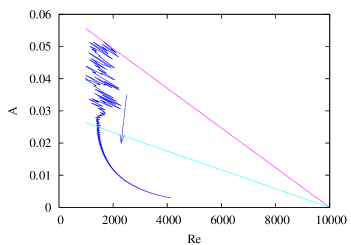
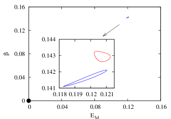
(a) (b)
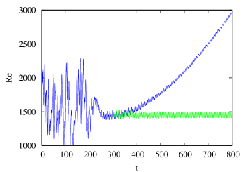
(c) (d)

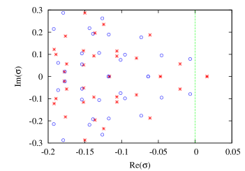
Figure 4: Application of the feedback control with $L=25D$, $m_{0}=2$ and mirror-symmetry imposed. (a) $(Re,A)$ representation. The arrow shows the direction of rotation of the slanted straight line, displayed here are two different times (b) time series of $Re(t)$ with time-varying (blue) and constant (green) $\kappa(t)$ for the stabilisation of the RPO. (c) $(E_{3d},\beta)$ representation of the RPO converged using the feedback control (red), the unstable RPO of the uncontrolled system (blue) at $Re=1450$, close to each other relative to the laminar state (black circle). (d) Spectrum of Floquet exponents for the RPO solution with (blue circles) and without control (red crosses).

4.3 Short periodic pipe with $m_{0}$=1

Bisections in periodic pipes without any rotational symmetry imposed ($m_{0}=1$) have been performed (Schneider et al., 2007; Duguet et al., 2008b) but to date no edge state with a simple dynamics has been reported for this case – the dynamics on the edge remains chaotic. Here we apply mirror symmetry to an $m_{0}=1$ computation in a short pipe with $\alpha=1.25$. The control by itself did not stabilise any TW solution in this case, but the dynamics on the edge is substantially less chaotic than the turbulent state. A narrow window of unsteady yet quiescent dynamics of the controlled system was identified in figure 5(a) near the intersection with the indicated straight line. Taking the state at this point as an initial guess in a Newton search converged to a new TW solution at $Re=2680$, whose cross-section and eigenvalue spectrum are displayed in figures 5(b)-(c), respectively. Note that this new TW does not satisfy the shift-and-reflect symmetry. It is characterised by one real unstable eigenvalue and one pair of complex unstable eigenvalues. Using the control the real eigenvalue is stabilised, and the resulting solution becomes only weakly unstable.

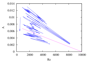
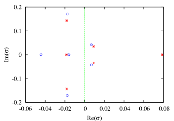
(a) (b)
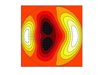
(c) (d)

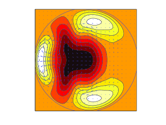
Figure 5: Application of the feedback control with $\alpha=1.25$, $m_{0}=1$. (a) $(Re,A)$ representation. The arrow shows the direction of rotation of the slanted straight line, which is displayed at the time where an approach to an unstable TW is identified (b) Cross-section of the stabilised TW solution (same colour coding as in figure 3), $Re=2680$. 3. (c) Eigenvalue spectrum for the TW solution with (blue circles) and without control (red crosses). (d) Cross-section after arc-lebgth continuation to $Re=1428$, $\alpha=1.25$.

Also shown is a cross-section of the solution after numerical continuation to $Re=1428$, where the solution appears in a saddle-node bifurcation at this $\alpha=1.25$.

5 Conclusions

We have demonstrated that the present feedback control method is able to stabilise invariant solutions that are edge states of the uncontrolled pipe flow system. Stabilised travelling waves correspond also to solutions of the uncontrolled Navier-Stokes equations. The control strategy is thus non-invasive in the case where the edge state of the original system is a travelling wave (Sieber et al., 2014). Relative periodic orbits or chaotic regimes stabilised using the method, however, are not precisely invariant solutions of the uncontrolled Navier–Stokes equations, but are expected to be sufficiently close for rapid continuation towards the original system. In both cases, the feedback control method proves very efficient at bringing the system close to the original edge state in only one short computation, whereas the same task using the bisection method would require $O(100)$ times as many simulations.

A similar feedback control has recently been considered for turbulence in stratified plane Couette flow (Taylor et al., 2016) to attain a target energy. The target energy may match that of the invariant solutions, which is not known a priori in such large domains.

Coupled with a Newton–Krylov solver, this new method, thanks to its low cost, can be used to probe the bifurcation diagram of the original system and explore the edge manifold without prior bisection. Adapting this method to other parallel shear flows, or to any other spatiotemporal system with hysteresis, is straightforward. Since one run is sufficient to uncover the whole lower branch parametrised by $Re$ (or potentially another parameter such as e.g. $\alpha$ or an additional force), it can either be used to perform wider parametric studies, or to identify the interesting regimes within the edge when multiple bifurcations occur (Khapko et al., 2014). We recommend implementation of the present control scheme as a simple precursor to the more expensive bisection and complex Newton–Krylov implementation.