A Riemannian trust-region method for low-rank tensor completion

Abstract

The goal of tensor completion is to fill in missing entries of a partially known tensor (possibly including some noise) under a low-rank constraint. This may be formulated as a least-squares problem. The set of tensors of a given multilinear rank is known to admit a Riemannian manifold structure, thus methods of Riemannian optimization are applicable.

In our work, we derive the Riemannian Hessian of an objective function on the low-rank tensor manifolds using the Weingarten map, a concept from differential geometry. We discuss the convergence properties of Riemannian trust-region methods based on the exact Hessian and standard approximations, both theoretically and numerically. We compare our approach to Riemannian tensor completion methods from recent literature, both in terms of convergence behaviour and computational complexity. Our examples include the completion of randomly generated data with and without noise and recovery of multilinear data from survey statistics.

1 Introduction

In this paper, we discuss optimization techniques on the manifold of tensors of a given rank. We consider least-squares problems of the form

$$\begin{split}&\min_{\mathbf{X}}\,f(\mathbf{X})=\frac{1}{2}\big{\lVert}\operatorname{P}_{\varOmega}\mathbf{X}-\operatorname{P}_{\varOmega}\mathbf{A}\big{\rVert}^{2}\\ \text{s.\,t.}\leavevmode\nobreak\ &\mathbf{X}\in{\mathcal{M}_{\mathbf{r}}}\coloneqq\big{\{}\mathbf{X}\in{\mathbb{R}}^{n_{1}\times\dotsb\times n_{d}}\,\big{|}\,\operatorname{rank}(\mathbf{X})=\mathbf{r}\big{\}},\end{split}$$ (1.1)

where $\operatorname{rank}(\mathbf{X})\in{\mathbb{R}}^{d}$ denotes the multilinear rank of a tensor $\mathbf{X}$, and $\operatorname{P}_{\varOmega}:{\mathbb{R}}^{n_{1}\times\dotsb\times n_{d}}\rightarrow{\mathbb{R}}^{n_{1}\times\dotsb\times n_{d}}$ is a linear operator. A typical choice found in the literature is

$$[\operatorname{P}_{\varOmega}\mathbf{X}]_{i_{1}\dotsc i_{d}}\coloneqq\begin{cases}x_{i_{1}\dotsc i_{d}}&\text{if\leavevmode\nobreak\ }(i_{1},\dotsc,i_{d})\in\varOmega,\\ 0&\text{otherwise},\end{cases}$$

where $\varOmega\subset\{1,\dotsc,n_{1}\}\times\dotsb\times\{1,\dotsc,n_{d}\}$ denotes the sampling set, i. e. we assume that ${\mathbf{A}\in{\mathbb{R}}^{n_{1}\times\dotsb\times n_{d}}}$ is a tensor whose entries with indices in $\varOmega$ are known.

The tensor completion problem is a generalization of the matrix completion problem, see the page by Ma et al. [1] for an overview of methods and applications in the context of convex optimization. Early work on tensor completion has been done by Liu et al. [2], who consider the problem

$$\min_{\mathbf{X}}\,\lVert\mathbf{X}\rVert_{*}\text{\;\;\;s.\,t.\;\,}\operatorname{P}_{\varOmega}\mathbf{X}=\operatorname{P}_{\varOmega}\mathbf{A}$$ (1.2)

in the context of image data recovery, where $\lVert\,\cdot\,\rVert_{*}$ is a generalized nuclear norm. Note that (1.2) can be viewed as the dual of (1.1). It ensures convexity for the tensor completion problem at the cost of losing the underlying manifold structure of low-rank tensors. Specifically, it does not give a low-rank solution in the presence of noise, i. e. if $\mathbf{A}\notin{\mathcal{M}_{\mathbf{r}}}$; in this case, an additional routine may be needed to truncate the result to low rank. Signoretto et al. [3] and Gandy et al. [4] choose a Tikhonov-like approach by minimizing the a penalized unconstrained function

$$\min_{\mathbf{X}}\,\frac{1}{2}\big{\lVert}\operatorname{P}_{\varOmega}\mathbf{X}-\operatorname{P}_{\varOmega}\mathbf{A}\big{\rVert}^{2}+\frac{\mu}{2}\lVert\mathbf{X}\rVert_{*}.$$

A Riemannian CG method for (1.1) has been proposed by Kressner et al. [5], which is an extension of Vandereycken’s earlier work [6] for the matrix completion problem. The authors show rapid linear convergence of their method with satisfactory reconstruction of missing data for a range of applications. Other Riemannian approaches for matrix completion include the work by Ngo/Saad [7] and Mishra et al. [8], who use a product Graßmann quotient manifold structure.

In recent research, second-order methods in Riemannian optimization have generated considerable interest in order to find superlinearly converging methods, see the overview by Absil et al. [9, Chapters 6–8] and the references therein. Boumal/Absil [10] apply these techniques to matrix completion in the Graßmannian framework. Vandereycken [6, Subsection 2.3] derives the Hessian for Riemannian matrix completion with an explicit expression of the singular values. In the higher-order tensor case, Eldén/Savas [11] propose a Newton method for computing a rank-$\mathbf{r}$ tensor approximation, using a Graßmannian approach. Ishteva et al. [12] extend these ideas to construct a Riemannian trust-region scheme.

In this paper, we propose a Riemannian trust-region scheme for (1.1) using explicit Tucker decompositions and compare it to a state-of-the-art Riemannian CG as used in [5]. We derive the exact expression of the Riemannian Hessian on ${\mathcal{M}_{\mathbf{r}}}$ for this manifold geometry by using the Weingarten map proposed by Absil et al. [13]. Our work focuses on the application case of tensor completion and contains tensor approximation as the special case of full sampling, i. e. $|\varOmega|=\prod_{i}n_{i}$.

The rest of the paper is organized as follows. In Section 2, we cite some basic results about tensor arithmetic and the manifold of low-rank tensors. In Section 3, we present a brief overview of Riemannian optimization and prove our main result, the Riemannian Hessian on ${\mathcal{M}_{\mathbf{r}}}$. In Section 4, we explain the Riemannian trust-region methods based on exact and approximate Hessian evaluations. In Section 5, we present the some numerical experiments for our method on synthetic data and a standard test data set from multilinear statistics.

2 Low-rank tensors

In this section, we collect some basic concepts and results on the Tucker decomposition and multilinear rank of tensors needed for our work. First, we define notations and results of general tensor arithmetic, as laid out in the survey paper [14]. Then, we introduce the manifold geometry of ${\mathcal{M}_{\mathbf{r}}}$, see [15, 16, 5].

2.1 Multilinear rank and Tucker decomposition

For a tensor $\mathbf{A}\in{\mathbb{R}}^{n_{1}\times\dotsb\times n_{d}}$, the matrix

$$A_{(i)}\in{\mathbb{R}}^{n_{i}\times\prod_{j\neq i}n_{j}},$$

such that the row index of $A_{(i)}$ is the $i$th modes of $\mathbf{A}$ and the column index is a multi-index of the remaining $d-1$ modes, in lexicographic order, is called the mode-$i$ matricization of $\mathbf{A}$. It may be viewed as a $d$-order generalization of the matrix transpose, since, for $d=2$, it holds that $A_{(1)}=A$ and $A_{(2)}=A^{\mathrm{T}}$. We denote the re-tensorization of a matricized tensor by a superscript index, i. e. $(A_{(i)})^{(i)}=\mathbf{A}$.

The multilinear rank of a tensor $\mathbf{A}$ is the $d$-tuple

$$\operatorname{rank}(\mathbf{A})=\big{(}\operatorname{rank}(A_{(1)}),\dotsc,\operatorname{rank}(A_{(d)})\big{)},$$

with $\operatorname{rank}(\,\cdot\,)$ on the right-hand side of the equation denoting the matrix rank. In contrast to the matrix case, the ranks of different matricizations of a tensor may be different, e. g. consider $\mathbf{A}\in{\mathbb{R}}^{2\times 2\times 2}$, given by its mode-$1$ matricization

$$A_{(1)}=\begin{bmatrix}1&0&0&0\\ 0&1&0&0\end{bmatrix}.$$

Then, the other matricizations are

$$A_{(2)}=A_{(1)},\leavevmode\nobreak\ A_{(3)}=\begin{bmatrix}1&0&0&1\\ 0&0&0&0\end{bmatrix},$$

so clearly $\operatorname{rank}(\mathbf{X})=(2,2,1)$.

The $i$-mode product of $\mathbf{A}$ with a matrix $M\in{\mathbb{R}}^{m\times n_{i}}$ is defined as

$$\mathbf{B}=\mathbf{A}\times_{i}M\iff B_{(i)}=MA_{(i)},\leavevmode\nobreak\ \mathbf{B}\in{\mathbb{R}}^{n_{1}\times\dotsb\times n_{i-1}\times m\times n_{i+1}\dotsb\times n_{d}}.$$

It is worth noting that, for different modes, the order of multiplications is irrelevant, i. e.

$$\mathbf{A}\times_{i}M\times_{j}N=\mathbf{A}\times_{j}N\times_{i}M\text{\;\;\;if\;\,}i\neq j.$$ (2.1)

If the modes are equal, then

$$\mathbf{A}\times_{i}M\times_{i}N=\mathbf{A}\times_{i}(NM).$$ (2.2)

A Frobenius inner product on ${\mathbb{R}}^{n_{1}\times\dotsb\times n_{d}}$ is given by

$$\langle\mathbf{A},\mathbf{B}\rangle\coloneqq\operatorname{tr}\big{(}A_{(1)}^{\mathrm{T}}B_{(1)}\big{)}=\dotsb=\operatorname{tr}\big{(}A_{(d)}^{\mathrm{T}}B_{(d)}\big{)}=\sum_{i_{1}=1}^{n_{1}}\dotsi\sum_{i_{d}=1}^{n_{d}}a_{i_{1}\dotso i_{d}}b_{i_{1}\dotso i_{d}},$$

with the induced norm $\lVert\mathbf{A}\rVert\coloneqq\sqrt{\langle\mathbf{A},\mathbf{A}\rangle}$.

A tensor $\mathbf{X}$ with $\operatorname{rank}(\mathbf{X})=\mathbf{r}=(r_{1},\dotsc,r_{d})$ can be represented in the Tucker decomposition [17]

$$\mathbf{X}=\mathbf{C}\times_{1}U_{1}\dotsb\times_{d}U_{d}=\mathbf{C}\bigtimes_{i=1}^{d}U_{i},$$ (2.3)

with a core tensor $\mathbf{C}\in{\mathbb{R}}^{r_{1}\times\dotsb\times r_{d}}$ with $\operatorname{rank}(\mathbf{C})=\mathbf{r}$ and basis matrices $U_{i}\in{\mathbb{R}}^{n_{i}\times r_{i}}$ with linearly independent columns. Without loss of generality, it can be assumed that the basis matrices have orthonormal columns, i. e. $U_{i}^{\mathrm{T}}U_{i}=I$. If for some $i$ this is not the case, a QR factorization $U_{i}=\widetilde{U}_{i}R$, with $\widetilde{U}_{i}$ orthonormal and $R$ regular and $\widetilde{\mathbf{C}}=(RC_{(i)})^{(i)}$ gives the required property.

A rank-$\mathbf{r}$ approximation to a tensor $\mathbf{A}$ can be computed by the truncated higher-order SVD (HOSVD) [18]: Let $\operatorname{P}_{r_{i}}^{i}$ be a the best rank-$r_{i}$ approximation operator in the $i$th mode, i. e. $\operatorname{P}_{r_{i}}^{i}\mathbf{A}=(U_{i}U_{i}^{\mathrm{T}}A_{(i)})^{(i)}$, where $U_{i}$ denotes the matrix of the $r_{i}$ dominant left singular vectors of $A_{(i)}$. Then the rank-$\mathbf{r}$ truncated HOSVD operator $\operatorname{P}_{\mathbf{r}}^{\mathrm{HO}}$ is given by

$$\operatorname{P}_{\mathbf{r}}^{\mathrm{HO}}\mathbf{A}\coloneqq\operatorname{P}_{r_{1}}^{1}\dotsm\operatorname{P}_{r_{d}}^{d}\mathbf{A}.$$ (2.4)

In contrast to the matrix case, the HOSVD does not yield a best rank-$\mathbf{r}$ approximation, but only a quasi-best-approximation [18, Property 10] with a constant which deteriorates with respect to the number of modes:

$$\big{\lVert}\mathbf{A}-\operatorname{P}_{\mathbf{r}}^{\mathrm{HO}}\mathbf{A}\big{\rVert}\leq\sqrt{d}\min_{\mathbf{X}\in{\mathcal{M}}_{\mathbf{r}}}\lVert\mathbf{A}-\mathbf{X}\rVert.$$ (2.5)

2.2 Riemannian manifold structure

In [15], the authors show that the set ${\mathcal{M}}_{\mathbf{r}}$ of tensors of fixed multilinear rank $\mathbf{r}=(r_{1},\dotsc,r_{d})$ forms a smooth embedded submanifold of ${\mathbb{R}}^{n_{1}\times\dotsb\times n_{d}}$. By counting the degrees of freedom in (2.3), it follows that

$$\dim({\mathcal{M}_{\mathbf{r}}})=\prod_{i=1}^{d}r_{i}+\sum_{i=1}^{d}r_{i}n_{i}-r_{i}^{2},$$

where the last term accounts for the fact that the Tucker decomposition is invariant to simultaneous transformation of the basis matrix with an invertible matrix and the core tensor with its inverse; as described in the previous subsection. Being a submanifold of the Euclidean space $({\mathbb{R}}^{n_{1}\times\dotsb\times n_{d}},\langle\,\cdot\,,\,\cdot\,\rangle)$, the manifold ${\mathcal{M}_{\mathbf{r}}}$ can be endowed with a Riemannian structure in a natural way with the Frobenius inner product $\langle\,\cdot\,,\,\cdot\,\rangle$ as the Riemannian metric.

As is proven in [16, Subsection 2.3], the tangent space of ${\mathcal{M}_{\mathbf{r}}}$ at $\mathbf{X}=\mathbf{C}\bigtimes_{i=1}^{d}U_{i}$ is parametrized as

$$T_{\mathbf{X}}{\mathcal{M}_{\mathbf{r}}}=\bigg{\{}\dot{\mathbf{C}}\bigtimes_{i=1}^{d}U_{i}+\sum_{i=1}^{d}\mathbf{C}\times_{i}\dot{U}_{i}\bigtimes_{j\neq i}U_{j}\,\bigg{|}\,\dot{\mathbf{C}}\in{\mathbb{R}}^{r_{1}\times\dotsb\times r_{d}},\leavevmode\nobreak\ \dot{U}_{i}\in{\mathbb{R}}^{n_{i}\times r_{i}}\text{\leavevmode\nobreak\ with\leavevmode\nobreak\ }\dot{U}_{i}^{\mathrm{T}}U_{i}=O\bigg{\}},$$ (2.6)

and the orthogonal projection $\operatorname{P}_{\mathbf{X}}:{\mathbb{R}}^{n_{1}\times\dotsb\times n_{d}}\rightarrow T_{\mathbf{X}}{\mathcal{M}_{\mathbf{r}}}$ is given by

$$\mathbf{A}\mapsto\bigg{(}\mathbf{A}\bigtimes_{j=1}^{d}U_{j}^{\mathrm{T}}\bigg{)}\bigtimes_{i=1}^{d}U_{i}+\sum_{i=1}^{d}\mathbf{A}\times_{i}\Bigg{(}\operatorname{P}_{U_{i}}^{\perp}\bigg{[}\mathbf{A}\bigtimes_{j\neq i}U_{j}^{\mathrm{T}}\bigg{]}_{(i)}C_{(i)}^{+}\Bigg{)}\bigtimes_{k\neq i}U_{k},$$ (2.7)

where $C_{(i)}^{+}$ denotes the Moore-Penrose pseudoinverse of $C_{(i)}$. Note that $C_{(i)}$ has full row rank, i. e. $C_{(i)}^{+}=C_{(i)}^{\mathrm{T}}(C_{(i)}C_{(i)}^{\mathrm{T}})^{-1}$. We use $\operatorname{P}_{U_{i}}^{\perp}=I_{n_{i}}-U_{i}U_{i}^{\mathrm{T}}$ to denote the orthogonal projection onto $\operatorname{span}(U_{i})^{\perp}$.

Furthermore, it can be shown that the HOSVD (2.4) is locally a $C^{\infty}$ function in the manifold topology of ${\mathcal{M}_{\mathbf{r}}}$, see [5, Proposition 2.1] for further details. This allows us its use in continuous optimization, as we will se in the next section.

3 The geometry of ${\mathcal{M}_{\mathbf{r}}}$ and Riemannian optimization

To construct optimization methods on ${\mathcal{M}_{\mathbf{r}}}$, we collect some basic concepts from the theory of optimization on manifolds. Our exposition follows the overview book [9]. Furthermore, we need to define and calculate the first and second derivatives of functions on ${\mathcal{M}_{\mathbf{r}}}$. In Corollary 3.7, we prove our main result, an explicit expression for the Riemannian Hessian on ${\mathcal{M}_{\mathbf{r}}}$. In the following, we will denote a Riemannian manifold by ${\mathcal{M}}$ and its elements by $x,y,\dotsc\in{\mathcal{M}}$, when citing general results, and the manifold of tensors of fixed multilinear rank by ${\mathcal{M}_{\mathbf{r}}}$ and its elements by $\mathbf{X},\mathbf{Y},\dotsc\in{\mathcal{M}_{\mathbf{r}}}$.

3.1 Retraction and vector transport

Since a manifold is in general not a linear space, the calculations required for a continuous optimization method need to be performed in a tangent space. Therefore, in each step, the need arises to map points from a tangent space to the manifold in order to generate the new iterate. The theoretically superior choice of such a mapping is the exponential map, which moves a point $x$ on the manifold along the geodesic locally defined by a vector in the tangent space $T_{x}{\mathcal{M}}$. However, computing the exponential map is prohibitively expensive in most situations, and it is shown in [9] that a first-order approximation, as specified in the following definition, is sufficient for many convergence results.

Definition 3.1.

A retraction on a manifold ${\mathcal{M}}$ is a smooth mapping $R$ from the tangent bundle $T{\mathcal{M}}$ onto ${\mathcal{M}}$ with the following properties. Let $R_{x}$ denote the restriction of $R$ to $T_{x}{\mathcal{M}}$.

1. $R_{x}(0_{x})=x$, where $0_{x}$ denotes the zero element of $T_{x}{\mathcal{M}}$.

2. With the canonical identification $T_{0_{x}}T_{x}{\mathcal{M}}\simeq T_{x}{\mathcal{M}}$, the mapping $R_{x}$ satisfies the rigidity condition

   $$\operatorname{D}R_{x}(0_{x})=\mathrm{id}_{T_{x}{\mathcal{M}}},$$

   where $\mathrm{id}_{T_{x}{\mathcal{M}}}$ denotes the identity mapping on $T_{x}{\mathcal{M}}$.

Furthermore, “comparing” tangent vectors at distinct points on the manifold will be useful. The following definition gives us a way to transport a tangent vector $\xi\in T_{x}{\mathcal{M}}$ to the tangent space $T_{R_{x}(\eta)}{\mathcal{M}}$ for some $\eta\in T_{x}{\mathcal{M}}$ and some retraction $R$.

Definition 3.2.

A vector transport on a manifold ${\mathcal{M}}$ is a smooth mapping

$$T{\mathcal{M}}\oplus T{\mathcal{M}}\rightarrow T{\mathcal{M}}:(\eta,\xi)\mapsto\mathcal{T}_{\eta}(\xi),$$

satisfying the following properties for all $x\in{\mathcal{M}}$:

1. (Associated retraction) There exists a retraction $R$, called the retraction associated with $\mathcal{T}$, such that, for all $\eta,\xi$, it holds that $\mathcal{T}_{\eta}\xi\in T_{R_{x}(\eta)}{\mathcal{M}}$.

2. (Consistency) $\mathcal{T}_{0_{x}}\xi=\xi$ for all $\xi\in T_{x}{\mathcal{M}}$.

3. (Linearity) The mapping $\mathcal{T}_{\eta}:T_{x}{\mathcal{M}}\rightarrow T_{R_{x}(\eta)}{\mathcal{M}},\leavevmode\nobreak\ \xi\mapsto\mathcal{T}_{\eta}\xi$ is linear.

For ${\mathcal{M}}={\mathcal{M}_{\mathbf{r}}}$, a retraction is given by the HOSVD, i. e. $R_{\mathbf{X}}(\xi)=\operatorname{P}_{\mathbf{r}}^{\mathrm{HO}}(\mathbf{X}+\xi)$. This is a consequence of the smoothness of the HOSVD (cf. Subsection 2.2) and the quasi-best approximation property (2.5). Details may be found in [5, Proposition 3]. A vector transport associated with a retraction $R$ is given by the orthogonal projection onto the tangent space, i. e. $\mathcal{T}_{\eta}(\xi)=\operatorname{P}_{R_{\mathbf{X}}(\eta)}(\xi)$, see [9, Subsection 8.1.3]; in our case, this is the formula (2.7). The efficient implementation of these operations is discussed in [5, Subsections 3.3–3.4]. A geometrical interpretation is shown in Figure 1.

Figure 1: Retraction (left) and vector transport (right) on ${\mathcal{M}_{\mathbf{r}}}$.

3.2 The Riemannian gradient

The low-rank Tucker manifold ${\mathcal{M}_{\mathbf{r}}}$ being a submanifold a Euclidean space, the gradient of a real-valued function defined on it can be easily calculated by projecting the Euclidean gradient onto the tangent space.

Lemma 3.3.

[9, Section 3.6.1] Let ${\mathcal{M}}$ be a Riemannian submanifold of a Euclidean space $E$. Let $\bar{f}:E\rightarrow{\mathbb{R}}$ be a function with Euclidean gradient $\operatorname{grad}\bar{f}(x)$ at point $x\in{\mathcal{M}}$. Then the Riemannian gradient of $f\coloneqq\bar{f}|_{\mathcal{M}}$ is given by $\operatorname{grad}f(x)=\operatorname{P}_{x}\operatorname{grad}\bar{f}(x)$, where $\operatorname{P}_{x}$ denotes the orthogonal projection onto the tangent space $T_{x}{\mathcal{M}}$.

Then, by Lemma 3.3, the Riemannian gradient of the tensor completion cost function is given by

$$\operatorname{grad}f(\mathbf{X})=\operatorname{P}_{\mathbf{X}}(\operatorname{P}_{\varOmega}\mathbf{X}-\operatorname{P}_{\varOmega}\mathbf{A}).$$ (3.1)

Using the sparsity of $\operatorname{P}_{\varOmega}\mathbf{X}-\operatorname{P}_{\varOmega}\mathbf{A}$, a gradient evaluation requires $\mathcal{O}(r^{d}(|\varOmega|+n)+r^{d+1})$ operations, cf. [5, Subsection 3.1], where we assume that the $r_{i}$ and $n_{i}$ are constant in each mode for simplicity of notation.

3.3 The Riemannian Hessian

By definition, the Riemannian Hessian of a real-valued function $f$ on a Riemannian manifold ${\mathcal{M}}$ is a linear mapping

$$\operatorname{Hess}f(x)[\xi]=\nabla_{\xi}\operatorname{grad}f(x),$$ (3.2)

where $\nabla$ denotes the Riemannian connection on ${\mathcal{M}}$, cf. [9, Definition 5.5.1]. A finite-difference approximation can be defined in different ways. An intuitive formula is given by

$$H^{\mathrm{FD}}[\xi]=\frac{\mathcal{T}_{\xi}\operatorname{grad}f(R_{x}(h\xi))-\operatorname{grad}f(x)}{h},$$ (3.3)

see, for example, [9, Subsection 8.2.1]. However, such a mapping will in general not be linear [19], and should be applied with care, as theoretical understanding is yet incomplete.

On a Riemannian submanifold of a Euclidean space, the Riemannian connection is just the orthogonal projection of the directional derivative, i. e.

$$\operatorname{Hess}f(x)[\xi_{x}]=\operatorname{P}_{x}\big{(}\operatorname{D}\operatorname{grad}f(x)[\xi_{x}]\big{)},$$ (3.4)

and using Lemma 3.3, we get the following result.

Lemma 3.4.

[9, Section 5.3.3] Let ${\mathcal{M}}$ be a Riemannian submanifold of a Euclidean space $E$. Let $\bar{f}:E\rightarrow{\mathbb{R}}$ be a function with Euclidean gradient $\operatorname{grad}\bar{f}(x)$ at point $x\in{\mathcal{M}}$. Then the Riemannian Hessian of $f\coloneqq\bar{f}|_{\mathcal{M}}$ is given by

$$\operatorname{Hess}f(x)[\xi_{x}]=\operatorname{P}_{x}\operatorname{D}\big{(}\operatorname{P}_{x}\operatorname{grad}\bar{f}(x)\big{)}.$$ (3.5)

Using the chain rule, we can write (3.5) as

$$\operatorname{Hess}f(x)[\xi] =\operatorname{P}_{x}\operatorname{D}\big{(}\operatorname{P}_{x}\operatorname{grad}\bar{f}(x)\big{)}$$

$$=\operatorname{P}_{x}\operatorname{Hess}\bar{f}(x)[\xi_{x}]+\operatorname{P}_{x}\operatorname{D}_{\xi}\operatorname{P}_{x}\operatorname{grad}\bar{f}(x),$$ (3.6)

where we view $x\mapsto\operatorname{P}_{x}$ as an operator-valued function and denote its directional derivative by $\operatorname{D}_{\xi}$. We observe that he first term in (3.6) is just the orthogonal projection of the Euclidean Hessian, while the second one depends on the curvature of the manifold ${\mathcal{M}}$. Indeed, the second term is equal to zero when ${\mathcal{M}}$ is flat, i. e. a linear subspace of the embedding Euclidean space, cf. [20, Subsection 4.1]. Clearly, the main challenge in calculating the Riemannian Hessian in (3.6) is the derivative of the projection operator. In [13, Section 3], the authors show the following result using the Weingarten map.

Lemma 3.5.

Let ${\mathcal{M}}$ be a Riemannian submanifold of a Euclidean space $\mathcal{E}$. For any $x\in{\mathcal{M}}$, let $\operatorname{P}_{x}$ denote the orthogonal projection onto the tangent space $T_{x}{\mathcal{M}}$, and $\operatorname{P}_{x}^{\perp}\coloneqq\operatorname{id}_{\mathcal{E}}-\operatorname{P}_{x}$ the orthogonal projection on its orthogonal complement $(T_{x}{\mathcal{M}})^{\perp}$. We view $x\mapsto\operatorname{P}_{x}$ as an operator-valued function and denote its Gâteaux derivative at point $x$ in the direction of $\xi\in T_{x}{\mathcal{M}}$ by $\operatorname{D}_{\xi}\operatorname{P}_{x}$. Then

$$\operatorname{P}_{x}\operatorname{D}_{\xi}\operatorname{P}_{x}u=\operatorname{P}_{x}\operatorname{D}_{\xi}\operatorname{P}_{x}\big{(}\operatorname{P}_{x}^{\perp}u\big{)},$$ (3.7)

for all $x\in{\mathcal{M}}$, $\xi\in T_{x}{\mathcal{M}}$ and $u\in\mathcal{E}$.

This result can be applied to the case of the low-rank Tucker manifold ${\mathcal{M}}={\mathcal{M}_{\mathbf{r}}}$. First, we calculate the derivative $\operatorname{D}_{\xi}\operatorname{P}_{\mathbf{X}}$.

Lemma 3.6.

Let $\mathbf{X}\in{\mathcal{M}_{\mathbf{r}}}$ be a tensor on the low-rank manifold, given by the factorization $\mathbf{X}=\mathbf{C}\bigtimes_{i=1}^{d}U_{i}$, and let $\xi\in T_{\mathbf{X}}{\mathcal{M}}_{\mathbf{r}}$, given by the variations

$$\xi=\dot{\mathbf{C}}\bigtimes_{i=1}^{d}U_{i}+\sum_{i=1}^{d}\mathbf{C}\times_{i}\dot{U}_{i}\bigtimes_{j\neq i}U_{j}.$$

We use the notations $\operatorname{P}_{U_{i}}=U_{i}U_{i}^{\mathrm{T}}$, $\operatorname{P}_{U_{i}}^{\perp}=I_{n_{i}}-U_{i}U_{i}^{\mathrm{T}}$ and $\dot{\operatorname{P}}_{U_{i}}=\dot{U}_{i}U_{i}^{\mathrm{T}}+U_{i}\dot{U}_{i}^{\mathrm{T}}$. Then, for any $\mathbf{E}\in{\mathbb{R}}^{n_{1}\times\dotsb\times n_{d}}$, the derivative of $\operatorname{P}_{\mathbf{X}}$ in the direction of $\xi$ is given by

$$\operatorname{D}_{\xi}\operatorname{P}_{\mathbf{X}}\mathbf{E}=\sum_{i=1}^{d}\Bigg{\{} \mathbf{E}\times_{i}\dot{\operatorname{P}}_{U_{i}}\bigtimes_{j\neq i}\operatorname{P}_{U_{j}}$$

$$+\, \dot{\mathbf{C}}\times_{i}\Bigg{(}\operatorname{P}_{U_{i}}^{\perp}\bigg{[}\mathbf{E}\bigtimes_{j\neq i}U_{j}^{\mathrm{T}}\bigg{]}_{(i)}C_{(i)}\Bigg{)}\bigtimes_{k\neq i}U_{k}$$

$$-\, \mathbf{C}\times_{i}\Bigg{(}\dot{\operatorname{P}}_{U_{i}}\bigg{[}\mathbf{E}\bigtimes_{j\neq i}U_{j}^{\mathrm{T}}\bigg{]}_{(i)}C_{(i)}\Bigg{)}\bigtimes_{k\neq i}U_{k}$$

$$+\, \sum_{l\neq i}\mathbf{C}\times_{i}\Bigg{(}\operatorname{P}_{U_{i}}^{\perp}\bigg{[}\mathbf{E}\times_{l}\dot{U}_{l}^{\mathrm{T}}\bigtimes_{l\neq j\neq i}U_{j}^{\mathrm{T}}\bigg{]}_{(i)}C_{(i)}\Bigg{)}\bigtimes_{k\neq i}U_{k}$$

$$+\, \mathbf{C}\times_{i}\Bigg{(}\operatorname{P}_{U_{i}}^{\perp}\bigg{[}\mathbf{E}\bigtimes_{j\neq i}U_{j}^{\mathrm{T}}\bigg{]}_{(i)}\bigg{[}\Big{(}I-C_{(i)}^{+}C_{(i)}\Big{)}\dot{C}_{(i)}^{\mathrm{T}}C_{(i)}^{+{\mathrm{T}}}C_{(i)}^{+}-C_{(i)}^{+}\dot{C}_{(i)}C_{(i)}^{+}\bigg{]}\Bigg{)}\bigtimes_{k\neq i}U_{k}$$

$$+\, \sum_{l\neq i}\mathbf{C}\times_{i}\Bigg{(}\operatorname{P}_{U_{i}}^{\perp}\bigg{[}\mathbf{E}\bigtimes_{j\neq i}U_{j}^{\mathrm{T}}\bigg{]}_{(i)}C_{(i)}\Bigg{)}\times_{l}\dot{U}_{l}\bigtimes_{l\neq k\neq i}U_{j}\Bigg{\}},$$

where $I=I_{\prod_{j\neq i}r_{j}}$ is the identity matrix of the appropriate size.

Proof.

The formula can be obtained by identifying the tensor $\mathbf{X}$ with the factors in the Tucker decomposition and viewing the orthogonal projection defined in (2.7) as a function

$$\operatorname{P}_{\,\cdot\,}\mathbf{E}:{\mathbb{R}}^{r_{1}\times\dotsb\times r_{d}}\times{\mathbb{R}}^{n_{1}\times r_{1}}\times\dotsb\times{\mathbb{R}}^{n_{d}\times r_{d}}\rightarrow{\mathbb{R}}^{n_{1}\times\dotsb\times n_{d}},\leavevmode\nobreak\ (\mathbf{C},U_{1},\dotsc,U_{d})\mapsto\operatorname{P}_{\mathbf{X}}\mathbf{E},$$

for any $\mathbf{E}\in{\mathbb{R}}^{n_{1}\times\dotsb\times n_{d}}$. For calculating the derivative of the pseudoinverse, we use the formula given in [21, Theorem 4.3], i. e.

$$\operatorname{D}_{\dot{C}}\big{(}C^{+}\big{)}=\big{(}I-C^{+}C\big{)}\dot{C}^{\mathrm{T}}C^{+{\mathrm{T}}}C^{+}+C^{+}C^{+{\mathrm{T}}}\dot{C}^{\mathrm{T}}\big{(}CC^{+}-I\big{)}-C^{+}\dot{C}C^{+},$$

and note that, here, the second term vanishes since $C=C_{(i)}$ has full row rank, and thus the pseudoinverse is a right inverse. ∎

Using this result, we can immediately evaluate the curvature term in (3.6).

Corollary 3.7.

We use the setting of Lemma 3.6 and denote the orthogonal projection onto $(T_{\mathbf{X}}{\mathcal{M}}_{\mathbf{r}})^{\perp}$ by $\operatorname{P}_{\mathbf{X}}^{\perp}\coloneqq\mathrm{id}-\operatorname{P}_{\mathbf{X}}$. Then

$$\operatorname{P}_{\mathbf{X}}\operatorname{D}_{\xi}\operatorname{P}_{\mathbf{X}}\operatorname{P}_{\mathbf{X}}^{\perp}\mathbf{E}=\widetilde{\mathbf{C}}\bigtimes_{i=1}^{d}U_{i}+\sum_{i=1}^{d}\mathbf{C}\times_{i}\widetilde{U}_{i}\bigtimes_{j\neq i}U_{j}\in T_{\mathbf{X}}{\mathcal{M}_{\mathbf{r}}},$$

with

$$\widetilde{\mathbf{C}} =\sum_{j=1}^{d}\bigg{(}\mathbf{E}\times_{j}\dot{U}_{j}^{\mathrm{T}}\bigtimes_{k\neq j}U_{k}^{\mathrm{T}}-\mathbf{C}\times_{j}\Big{(}\dot{U}_{j}^{\mathrm{T}}\big{[}\mathbf{E}\bigtimes_{k\neq j}U_{j}^{\mathrm{T}}\big{]}_{(j)}C_{(j)}^{+}\Big{)}\bigg{)},$$

$$\widetilde{U}_{i} =\operatorname{P}_{U_{i}}^{\perp}\bigg{(}\big{[}\mathbf{E}\bigtimes_{j\neq i}U_{j}^{\mathrm{T}}\big{]}_{(i)}\big{(}I-C_{(i)}^{+}C_{(i)}\big{)}\dot{C}_{(i)}^{\mathrm{T}}C_{(i)}^{+{\mathrm{T}}}+\sum_{k\neq i}\big{[}\mathbf{E}\times_{k}\dot{U}_{k}^{\mathrm{T}}\bigtimes_{k\neq j\neq i}U_{j}^{\mathrm{T}}\big{]}_{(i)}\bigg{)}C_{(i)}^{+},$$

Proof.

The result follows by applying Lemma 3.6 to $\operatorname{P}_{\mathbf{X}}^{\perp}\mathbf{E}\in{\mathbb{R}}^{n_{1}\times\dotsb\times n_{d}}$ after some lengthy but straightforward calculations, using the orthonormality relations $\dot{U}_{i}^{\mathrm{T}}U_{i}=O$, $U_{i}^{\mathrm{T}}U_{i}=I$ and the rules (2.1) and (2.2) for the matrix-tensor product. ∎

Thus, the Riemannian Hessian of the function $f:{\mathcal{M}_{\mathbf{r}}}\rightarrow{\mathbb{R}}$,

$$f(\mathbf{X})=\frac{1}{2}\big{\lVert}\operatorname{P}_{\varOmega}\mathbf{X}-\operatorname{P}_{\varOmega}\mathbf{A}\big{\rVert}^{2},$$

can be written as

$$\operatorname{Hess}f(\mathbf{X})[\xi]=\operatorname{P}_{\varOmega}(\xi)+\operatorname{P}_{\mathbf{X}}\operatorname{D}_{\xi}\operatorname{P}_{\mathbf{X}}\operatorname{P}_{\mathbf{X}}^{\perp}(\operatorname{P}_{\varOmega}\mathbf{X}-\operatorname{P}_{\varOmega}\mathbf{A})$$ (3.8)

and the second term can be evaluated with Corollary 3.7.

Note that for an efficient computation of the terms $\widetilde{U}_{i}$, it is advantageous to multiply out the term containing $I-C_{(i)}^{+}C_{(i)}$. Then, the computation of $\operatorname{Hess}f(\mathbf{X})[\xi]$ for any given $\xi\in T_{\mathbf{X}}{\mathcal{M}_{\mathbf{r}}}$ has the same complexity as the computation of the gradient, i. e. $\mathcal{O}(r^{d}(|\varOmega|+n)+r^{d+1})$.

Remark 3.8.

For the matrix case $d=2$, the Hessian expression (3.8) can be simplified to recover the expression shown in [6, 13],

$$\begin{split}\operatorname{Hess}f(X)[\xi]=&\operatorname{P}_{U}\operatorname{P}_{\varOmega}(\xi)\operatorname{P}_{V}+\operatorname{P}_{U}^{\perp}\big{[}\operatorname{P}_{\varOmega}(\xi)+\operatorname{P}_{\varOmega}(X-A)\dot{V}\varSigma^{-1}V^{\mathrm{T}}\big{]}\operatorname{P}_{V}\\ &+\operatorname{P}_{U}\big{[}\operatorname{P}_{\varOmega}(\xi)+U\varSigma^{-1}\dot{U}^{\mathrm{T}}\operatorname{P}_{\varOmega}(X-A)\big{]}\operatorname{P}_{V}^{\perp},\end{split}$$

where we identify the Tucker decomposition with the usual notation for the SVD, i. e. $U=U_{1}$, $V=U_{2}$ and $\varSigma=C$.

4 Riemannian models and trust-region methods

In principle, the results of the previous subsections can be used to conceive a Riemannian Newton method for the solution of problem (1.1). Such a method has been proposed in [22, pp. 279–283], where a convergence proof is given for strongly convex functions [22, Definition 1.1 in Chapter 7], using retraction by the exponential mapping (i. e. moving locally on a geodesic). [23, Theorem 4.4] proves quadratic convergence of the method to a critical point. [9, Theorem 6.3.2] provides a generalization for general retractions.

However, a plain Newton method has some well-known drawbacks:

1. The convergence radius may be small, i. e. if the initial guess is too far from a critical point the method may diverge.

2. Each step requires the solution of a linear system. This may be expensive and conceptually difficult if the Hessian operator is not even given explicitly but in terms of the action on a vector in the tangent space, as in (3.8).

There exists a number of strategies for remedying these problems. An intuitive method for globalizing the convergence of a Newton method is to modify the Hessian such that the solution $\xi$ of

$$\operatorname{Hess}f(x_{k})[\xi]=-\operatorname{grad}f(x_{k})$$ (4.1)

defines a descent direction, see [24, Section 3.4] for an overview in the Euclidean case. In [9, Section 6.2] a generalization to the Riemannian case is proposed, replacing the Newton equation with

$$\big{(}\operatorname{Hess}f(x_{k})+E_{k}\big{)}[\xi]=-\operatorname{grad}f(x_{k}),$$

where $E_{k}$ is a sequence of positive-definite linear operators on the tangent spaces $T_{x_{k}}{\mathcal{M}}$.

However, such perturbed Newton methods rely on heuristics, and their general convergence properties are not well understood. Moreover, they still require the solution of a linear system in each iteration. A way to circumvent this are trust-region methods [25], which find a critical point of the function $f$ by minimizing a sequence of constraint quadratic models $m_{x_{k}}$. Our exposition follows the generalization to Riemannian optimization as given by Absil et al. [26].

4.1 Models on a Riemannian manifold ${\mathcal{M}}$

For a real-valued function $f$ on a Riemannian manifold ${\mathcal{M}}$, a function $m_{x}$ is called an order-$q$ model, $q>0$, of ${\mathcal{M}}$ in $x\in{\mathcal{M}}$ if there exists a neighbourhood $\mathcal{U}$ of $x$ in ${\mathcal{M}}$ and a constant $c>0$ such that

$$\big{|}f(y)-m_{x}(y)\big{|}\leq c\big{(}\operatorname{dist}(x,y)\big{)}^{q+1},\text{\;\;\;for all\;\,}y\in\mathcal{U},$$

where $\operatorname{dist}$ denotes the Riemannian (geodesic) distance on ${\mathcal{M}}$. It can be shown [9, Proposition 7.1.3] that a model $m_{x}$ is order-$q$ if and only if there exists a neighbourhood $\mathcal{U}^{\prime}$ of $x$ in ${\mathcal{M}}$ and a constant $c^{\prime}>0$ such that

$$\big{|}f(y)-m_{x}(y)\big{|}\leq c\big{\|}R_{x}^{-1}(y)\big{\|}^{q+1},\text{\;\;\;for all\;\,}y\in\mathcal{U}.$$

i. e. the order of a model can be assessed using any retraction and we can avoid working with the exact geodesic.

Given a retraction $R$, this result allows to build a model for $f$ by simply taking a truncated Taylor expansion of

$$\widehat{f}_{x}\coloneqq f\circ R_{x},$$

for any $x\in{\mathcal{M}}$. The definition of $\widehat{f}_{x}:T_{x}{\mathcal{M}}\rightarrow{\mathbb{R}}$ as a real-valued function on a Euclidean space allows us to use standard results from multivariate analysis. A simple first-order model is then given by

$$\widehat{m}_{x}=\widehat{f}_{x}(0_{x})+\operatorname{D}\widehat{f}_{x}(0_{x})[\xi]=f(x)+\langle\operatorname{grad}f(x),\xi\rangle,$$

where the second equality follows form the rigidity condition of the retraction. A generic second-order model is given by

$$\widehat{m}_{x} =\widehat{f}_{x}(0_{x})+\operatorname{D}\widehat{f}_{x}(0_{x})[\xi]+\tfrac{1}{2}\operatorname{D}^{2}\widehat{f}_{x}(0_{x})[\xi,\xi]$$

$$=f(x)+\langle\operatorname{grad}f(x),\xi\rangle+\tfrac{1}{2}\big{\langle}\operatorname{Hess}\widehat{f}(x)[\xi],\xi\big{\rangle}.$$

A straightforward and useful modification is obtained by replacing the Euclidean Hessian on the tangent space $\operatorname{Hess}\widehat{f}(x)$ by the Riemannian expression $\operatorname{Hess}f(x)$. The following lemma shows that this can be done in a critical point of $f$ without any loss of information.

Lemma 4.1.

[9, Proposition 5.5.6] Let $R$ be a retraction and let $x^{*}$ be a critical point of a real-valued function $f$ on ${\mathcal{M}}$, i. e. $\operatorname{grad}f(x^{*})=0_{x^{*}}$. Then

$$\operatorname{Hess}f(x^{*})=\operatorname{Hess}\widehat{f}(0_{x^{*}}).$$

Thus, we can define a model

$$m_{x}=f(x)+\langle\operatorname{grad}f(x),\xi\rangle+\tfrac{1}{2}\big{\langle}\operatorname{Hess}f(x)[\xi],\xi\big{\rangle},$$

which does not make any use of a retraction. However, Lemma 4.1 only guarantees that $m_{x}$ matches $f$ up to second order if $x$ is a critical point. In general, we can only prove that it will only give us a first-order model. The model $m_{x}$ can be shown to be of second order for general $x$ if the retraction $R$ is of second order, i. e. if it preserves second-order information of the exponential map, cf. [9, Proposition 5.5.5]. However, numerical results presented later in this section suggest that in our case the result also holds for general points on the manifold.

4.2 Models of different orders on ${\mathcal{M}_{\mathbf{r}}}$

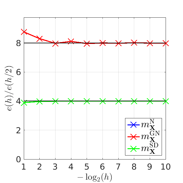
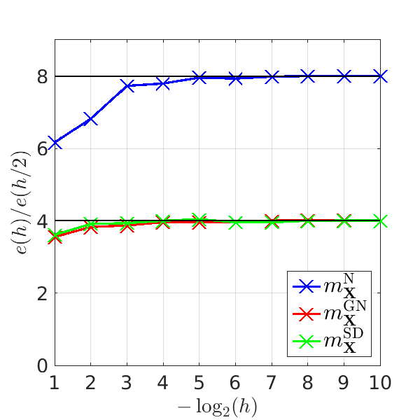
$f(\mathbf{X})=0$	$f(\mathbf{X})=1.2\times 10$
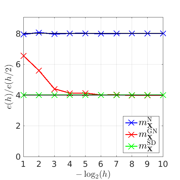
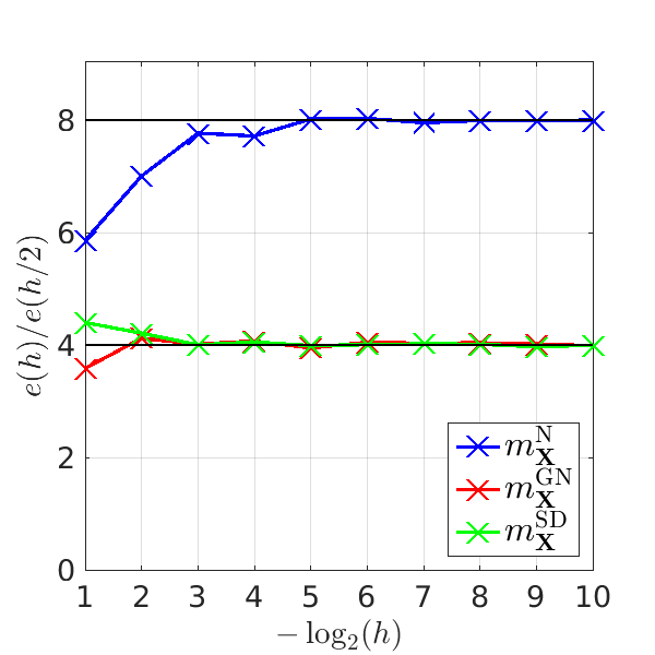
$f(\mathbf{X})=2.1\times 10^{-2}$	$f(\mathbf{X})=1.9\times 10^{2}$
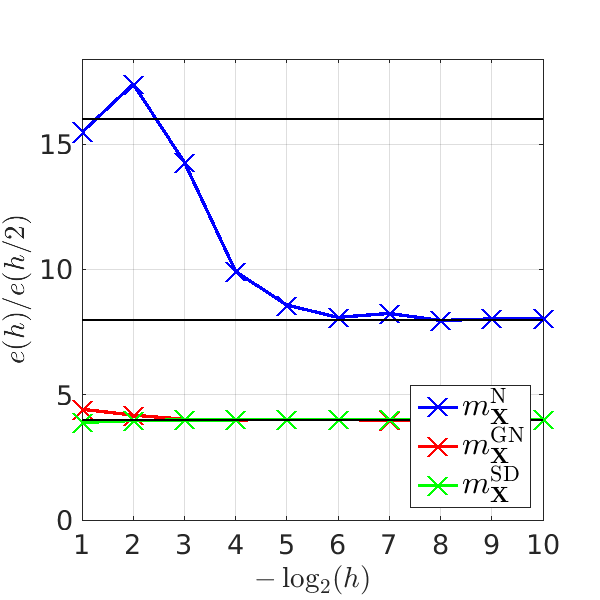
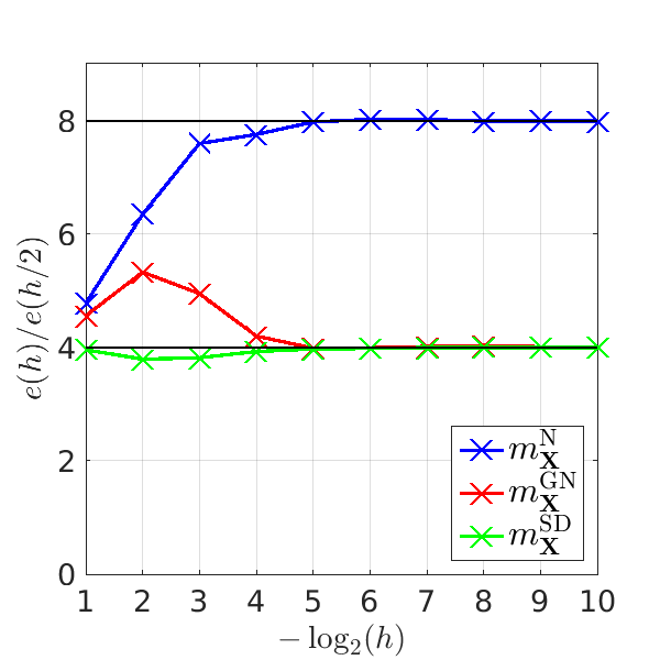
$f(\mathbf{X})=3.6\times 10^{2}$	$f(\mathbf{X})=1.8\times 10^{3}$

Figure 2: The unknown tensor $\mathbf{A}$ has full rank, i. e. $\mathbf{A}\notin{\mathcal{M}_{\mathbf{r}}}$.

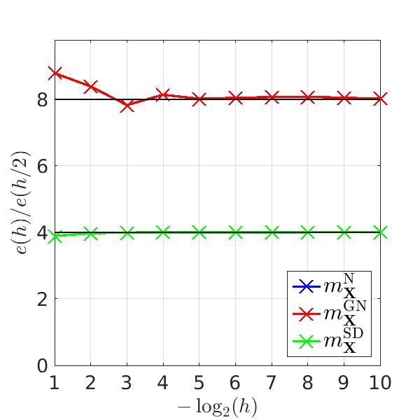
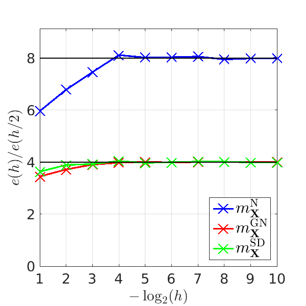
$f(\mathbf{X})=0$	$f(\mathbf{X})=1.3\times 10$
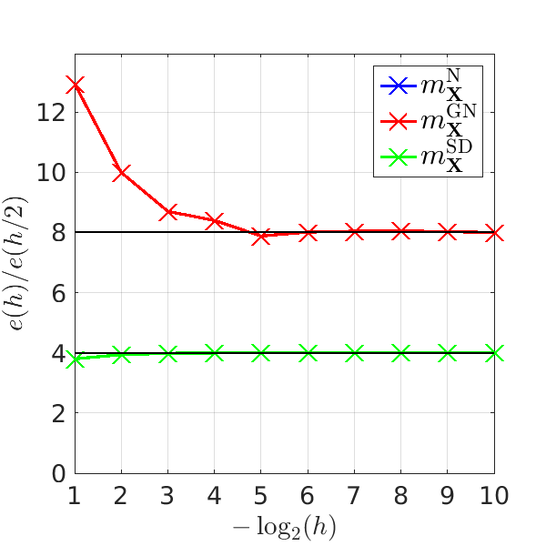
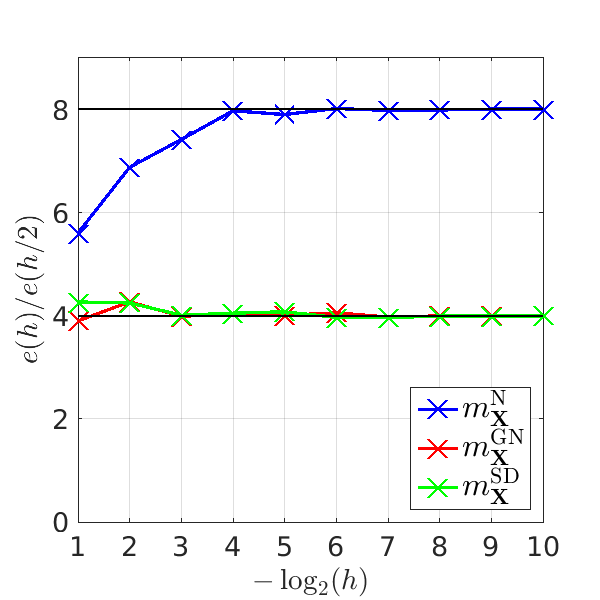
$f(\mathbf{X})=0$	$f(\mathbf{X})=1.5\times 10^{2}$
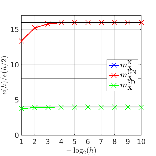
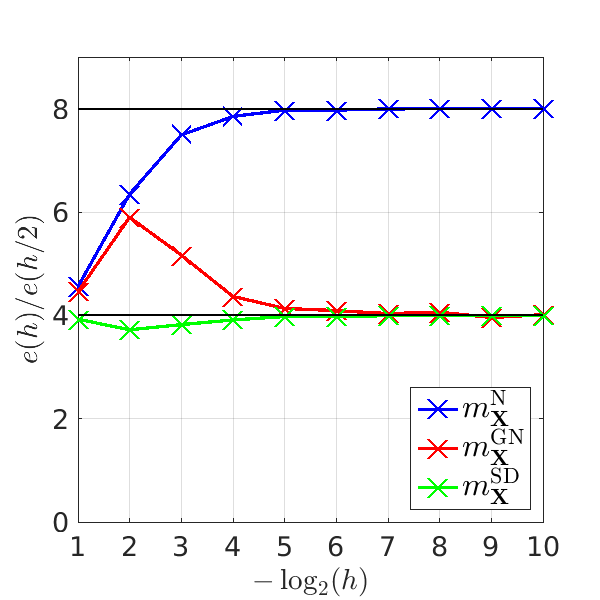
$f(\mathbf{X})=0$	$f(\mathbf{X})=1.4\times 10^{3}$

Figure 3: The unknown tensor $\mathbf{A}$ has low rank, i. e. $\mathbf{A}\in{\mathcal{M}_{\mathbf{r}}}$.

We consider the manifold ${\mathcal{M}_{\mathbf{r}}}$ of fixed-rank tensors and would like to assess the quality of different model functions. In accordance with the previous subsection, we consider a first-order model

$$m_{\mathbf{X}}^{\mathrm{SD}}(\xi)\coloneqq f(\mathbf{X})+\langle\operatorname{grad}f(\mathbf{X}),\xi\rangle,$$ (4.2)

where the superscript indicates that this model corresponds to a steepest-descent method, and a second-order model

$$m_{\mathbf{X}}^{\mathrm{N}}(\xi)\coloneqq f(\mathbf{X})+\langle\operatorname{grad}f(\mathbf{X}),\xi\rangle+\tfrac{1}{2}\big{\langle}\operatorname{Hess}f(\mathbf{X})[\xi],\xi\big{\rangle},$$

where the superscript indicates that this model corresponds to a Newton method. Furthermore, we would like to assess the quality of a Hessian approximation which drops the curvature term in Corollary 3.7 and thus ignores the second-order geometry of ${\mathcal{M}_{\mathbf{r}}}$. This is given by omitting the second term in (3.8), and just considering the projection of the Euclidean Hessian i. e.

$$\widetilde{\operatorname{Hess}}f(\mathbf{X})[\xi]=\operatorname{P}_{\varOmega}\xi.$$ (4.3)

Omitting the curvature term of the Hessian corresponds to a Riemannian Gauß–Newton method, as described in [9, Subsection 8.4.1]. Thus, we consider the model function

$$m_{\mathbf{X}}^{\mathrm{GN}}(\xi)\coloneqq f(\mathbf{X})+\langle\operatorname{grad}f(\mathbf{X}),\xi\rangle+\tfrac{1}{2}\big{\langle}\widetilde{\operatorname{Hess}}f(\mathbf{X})[\xi],\xi\big{\rangle}.$$ (4.4)

As usual, we can expect a Gauß–Newton method to converge superlinearly (as the corresponding model to be of order higher than $1$) if the residual of the least-squares problem is low. This can be seen in terms of (3.8), where the curvature term is given as

$$\big{(}\operatorname{Hess}f(\mathbf{X})-\widetilde{\operatorname{Hess}}f(\mathbf{X})\big{)}[\xi]=\operatorname{P}_{\mathbf{X}}\operatorname{D}_{\xi}\operatorname{P}_{\mathbf{X}}\operatorname{P}_{\mathbf{X}}^{\perp}(\operatorname{P}_{\varOmega}\mathbf{X}-\operatorname{P}_{\varOmega}\mathbf{A}),$$

which is clearly equal to zero if $\operatorname{P}_{\varOmega}\mathbf{X}=\operatorname{P}_{\varOmega}\mathbf{A}$ and hence $f(\mathbf{X})=0$.

To assess the order of a model, we define for a given $m_{\mathbf{X}}$ the model error

$$e(\xi,h)\coloneqq\big{|}\widehat{f}_{\mathbf{X}}(h\xi)-m_{\mathbf{X}}(h\xi)\big{|},$$

for $\xi\in T_{\mathbf{X}}{\mathcal{M}_{\mathbf{r}}}$ and $h\geq 0$. Then $m_{\mathbf{X}}$ is an order-$q$ model in $\mathbf{X}$ if and only if

$$e(\xi,h)=\mathcal{O}\big{(}h^{q+1}\big{)},\text{\;\;\;for all\;\,}\xi\in T_{\mathbf{X}}{\mathcal{M}_{\mathbf{r}}}.$$

In Figures 2 and 3, we test the model orders of (4.2)–(4.4). We generate random tensors $\mathbf{B}_{1},\dotsc,\mathbf{B}_{1000}\in{\mathbb{R}}^{10\times 10\times 10}$ with normally distributed entries and project them onto a given tangent space of ${\mathcal{M}}_{(3,3,3)}$ to get $\xi_{i}=\operatorname{P}_{\mathbf{X}}(\mathbf{B}_{i})$. We normalize the resulting vectors to get $\lVert\xi_{i}\rVert=1$. We compute the errors $e(\xi_{i},2^{-j})$ for $j=0,\cdots,10$, and plot the geometric mean of the factors $(\xi_{i},2^{-(j+1})/(\xi_{i},2^{-j})$ over all $i$. The first columns contain the results for a stationary point of $f$, i. e. $\lVert\operatorname{grad}f({\mathbf{X^{*}}})\rVert=0$, the second columns contain the results for an arbitrary point on the manifold with $\lVert\operatorname{grad}f(\mathbf{X})\rVert\neq 0$. The first, second and third rows contain results for different sampling sizes, with $|\varOmega|=10,100,1000$, respectively. Note that $|\varOmega|=1000$ represents full sampling, i. e. vector approximation. We write $f(\mathbf{X})=0$ whenever the function value computed is smaller that the machine precision of $10^{-16}$.

We observe that the model function $m_{\mathbf{X}}^{\mathrm{SD}}$, indeed, provides results of first order in all cases. The model function $m_{\mathbf{X}}^{\mathrm{N}}$ provides results of second order not only in critical points, as has been proved by theory, but also in general points on the manifold. This can be seen as an indication that the retraction by HOSVD preserves second-order information although we cannot prove this. We also observe that the Gauß–Newton type model function $m_{\mathbf{X}}^{\mathrm{GN}}$ gives second-order results whenever the curvature term is small enough, otherwise it is only a first-order model; this matches the theoretical predictions we made earlier. It is especially worth noting that, for $\mathbf{A}\in{\mathcal{M}_{\mathbf{r}}}$, a Gauß–Newton model is sufficient; however, this result is not robust if we add some noise. Note that in the cases where the blue curve cannot be seen in the plot, the models $m_{\mathbf{X}}^{\mathrm{GN}}$ and $m_{\mathbf{X}}^{\mathrm{N}}$ match almost exactly.

We also remark that in the case of exact tensor reconstruction, i. e. $\mathbf{A}\in{\mathcal{M}_{\mathbf{r}}}$ and ${|\varOmega|=\prod_{i}n_{i}}$ (the lower-left plot in Figure 3), both $m_{\mathbf{X}}^{\mathrm{N}}$ and $m_{\mathbf{X}}^{\mathrm{GN}}$ seem to be models of order $3$, which means that the third-order term in the Taylor expansion of $f$ vanishes. This may be attributed to a possible symmetry of $f$ around the local minimizer $\mathbf{X}^{*}=\mathbf{A}$ in this case, i. e. $f(\operatorname{Exp}_{\mathbf{X}^{*}}(\xi))=f(\operatorname{Exp}_{\mathbf{X}^{*}}(-\xi))$, where $\operatorname{Exp}$ denotes the exponential map. This means that the odd-exponent terms in the Taylor expansion are equal to zero. However, we cannot verify this theoretically as we do not have a closed-form expression for the exponential map on ${\mathcal{M}_{\mathbf{r}}}$.

4.3 Riemannian trust-region method

The main idea of trust-region methods is solving a model problem

$$\begin{split}&\min_{\eta\in T_{\mathbf{X}_{k}}{\mathcal{M}_{\mathbf{r}}}}m_{\mathbf{X}_{k}}(\eta)\\ \text{s.\,t.}\leavevmode\nobreak\ &\lVert\eta\rVert\leq\varDelta_{k},\end{split}$$ (4.5)

for some $\varDelta_{k}\geq 0$ in each iteration $k$ to obtain a search direction $\eta_{k}$. To get meaningful results it is crucial to check how well the model $m_{\mathbf{X}_{k}}$ approximates $\widehat{f}$ in $T_{\mathbf{X}_{k}{\mathcal{M}_{\mathbf{r}}}}$ in the neighbourhood of $0_{\mathbf{X}_{k}}$. This can be expressed in the form of the quotient

$$\rho_{k}\coloneqq\frac{\widehat{f}(0_{\mathbf{X}_{k}})-\widehat{f}(\eta_{k})}{m_{\mathbf{X}_{k}}(0_{\mathbf{X}_{k}})-m_{\mathbf{X}_{k}}(\eta_{k})}.$$ (4.6)

If $\rho_{k}$ is small (convergence theory suggests that $\rho^{\prime}<\tfrac{1}{4}$ is an appropriate threshold), then the model is very inaccurate: the step must be rejected, and the trust-region radius $\varDelta_{k}$ must be reduced. If $\rho_{k}$ is small but less dramatically so, then the step is accepted but the trust-region radius is reduced. If $\rho_{k}$ is close to 1, then there is a good agreement between the model and the function over the step, and the trust-region radius can be expanded. If $\rho_{k}\gg 1$, then the model is inaccurate, but the overall optimization iteration is producing a significant decrease in the cost. If this is the case and the restriction in (4.5) is active, we can try to expand the trust-region radius as long as we stay below a predefined bound $\bar{\varDelta}>0$. This method is summarized in Algorithm 4.2, cf. [26, Algorithm 1].

Algorithm 4.2 Riemannian trust-region method for ${\mathcal{M}_{\mathbf{r}}}$

1:Initial iterate $x_{0}\in{\mathcal{M}}$; parameters $\bar{\varDelta}>0$, $\varDelta_{0}\in(0,\bar{\varDelta})$, $\rho^{\prime}\in(0,\tfrac{1}{4})$.

2:for $k=0$ until convergence do

3:     Obtain $\eta_{k}$ by approximately solving (4.5)

4:     $<$Test for convergence$>$

5:     Evaluate $\rho_{k}$ from (4.6)

6:     if $\rho_{k}<\tfrac{1}{4}$ then

7:         $\varDelta_{k+1}=\tfrac{1}{4}\varDelta_{k}$

8:     else if $\rho_{k}>\tfrac{3}{4}$ and $\lVert\eta_{k}\rVert=\varDelta_{k}$ then

9:         $\varDelta_{k+1}=\min(2\varDelta_{k},\bar{\varDelta})$

10:     else

11:         $\varDelta_{k+1}=\varDelta_{k}$

12:     end if

13:     if $\rho_{k}>\rho^{\prime}$ then

14:         $\mathbf{X}_{k+1}=R_{\mathbf{X}_{k}}(\eta_{k})$

15:     else

16:         $\mathbf{X}_{k+1}=\mathbf{X}_{k}$

17:     end if

18:end for

There exist different strategies for (approximately) solving the trust-region subproblems (4.5). We apply a truncated CG method [26, Algorithm 2], which is a straightforward adaptation of Steighaug’s method [27] for problems in ${\mathbb{R}}^{n}$. It ensures that the CG method is stopped after a fixed maximal number of iterations $K_{\max}$. Since a CG iteration just requires a fixed number of matrix-vector products, the total cost of the trust-region method with exact Hessian evaluation is given by

$$\mathcal{O}\big{(}K_{\max}(r^{d}(|\varOmega|+n)+r^{d+1})\big{)}$$

The convergence theory follows standard techniques from Euclidean optimization [25]. Under some technical assumptions, it can be shown that Algorithm 4.2 converges globally to a stationary point [26, Theorem 4.4] of $f$. Locally superlinear convergence to a nondegenerate local minimum can be shown [26, Theorem 4.12] as long as the quadratic term in $m_{\mathbf{X}_{k}}$ is a sufficiently good Hessian approximation of $f$.

In general, we cannot rule out Algorithm 4.2 converging to a nonregular minimum if ${|\varOmega|<\dim({\mathcal{M}_{\mathbf{r}}})}$. If this causes problems, we can enforce positive-definiteness of the Hessian by considering a cost function regularized with an identity term

$$f_{\mu}(\mathbf{X})=\frac{1}{2}\big{\lVert}\operatorname{P}_{\varOmega}\mathbf{X}-\operatorname{P}_{\varOmega}\mathbf{A}\big{\rVert}^{2}+\frac{\mu}{2}\lVert\mathbf{X}\rVert^{2},$$

for some $\mu>0$. However, such a problem may not be well-posed since there is not enough information provided to recover $\mathbf{X}$ in a meaningful way. Moreover, in our practical experiments we did not have a need to use this regularization.

5 Numerical experiments

We implemented our method in Matlab version 2015b using the Tensor Toolbox version 2.6 [28, 29] for the basic tensor arithmetic and Manopt version 3.0 [30] for handling the Riemannian trust-region scheme. All tests were performed on a quad-core Intel i7-2600 CPU with 8 GB of RAM running 64-Bit Ubuntu 16.04 Linux.

In Algorithm 4.2, we choose the standard parameters $\bar{\varDelta}=\dim({\mathcal{M}_{\mathbf{r}}})$, $\varDelta_{0}=\bar{\varDelta}/8$, $\rho^{\prime}=0.1$. The initial guess $\mathbf{X}_{0}$ is generated randomly by a uniform distribution on $(0,1)$ for each entry in the factors in the Tucker decomposition. We apply a QR factorization in each mode to ensure that the basis matrices are orthogonal. The sampling set $\varOmega$ is chosen from a uniform distribution on the index set.

5.1 Uniformly distributed random data

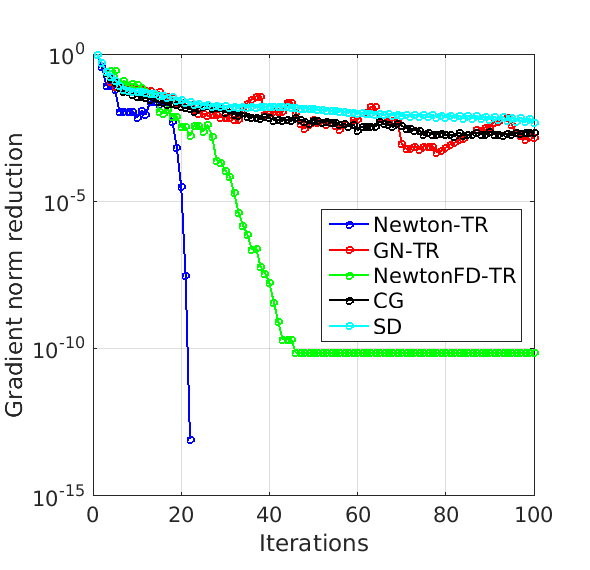
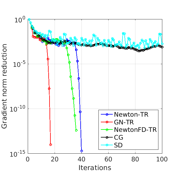
$|\varOmega|=0.05\times\prod_{i}n_{i}$, $\mathbf{A}\notin{\mathcal{M}_{\mathbf{r}}}$	$|\varOmega|=0.05\times\prod_{i}n_{i}$, $\mathbf{A}\in{\mathcal{M}_{\mathbf{r}}}$
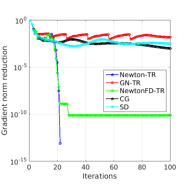
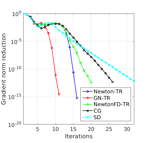
$|\varOmega|=0.5\times\prod_{i}n_{i}$, $\mathbf{A}\notin{\mathcal{M}_{\mathbf{r}}}$	$|\varOmega|=0.5\times\prod_{i}n_{i}$, $\mathbf{A}\in{\mathcal{M}_{\mathbf{r}}}$

Figure 4: Convergence of Riemannian methods for (1.1) with $n_{i}\equiv 20$ and $r_{i}\equiv 2$.

We test the convergence behaviour of Algorithm 4.2 for the recovery of a partially known tensor $\mathbf{A}$ with uniformly distributed entries. We observe that the trust-region method with exact Hessian computation yields superlinear convergence after a small number of iterations in all cases observed here. The finite difference Hessian approximation shows similar behaviour, however, the convergence is slower and becomes less reliable for a large gradient norm reduction. The Gauß–Newton Hessian approximation shows shows superlinear convergence behaviour if $\mathbf{A}\in{\mathcal{M}_{\mathbf{r}}}$, but not in the case $\mathbf{A}\notin{\mathcal{M}_{\mathbf{r}}}$, as predicted in the previous sections. The state-of-the-art Riemannian method, nonlinear CG [5], shows linear convergence with convergence rate superior to steepest descent, but the convergence rate may slow, especially in the case of noise.

5.2 Survey data

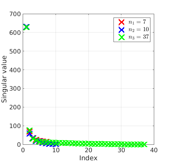
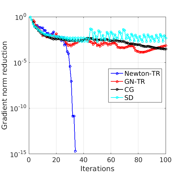
Figure 5: Left: Singular values of the data set [31]; right: convergence of Riemannian methods for tensor completion with $|\varOmega|=0.5\times\prod_{i}n_{i}$ and $\mathbf{r}=(3,5,5)$.

In survey statistics, data in the form of order-$3$ tensors arises in a natural way: for $n_{1}$ of individuals, $n_{2}$ properties are collected over $n_{3}$ time points; see, for example, [32]. We choose a standard data set [31], containing reading proficiency test measures of schoolchildren over a period of time. A typical problem in such data sets in practice is missing entries, resulting from nonresponse or failure to enter some of the data points correctly; see [33]. A typical application case is a sampling set greater or equal to haf the total tensor size. As Figure 5 shows, data of this type shows rapidly decaying singular values, especially in the time mode ($i=3$) and our trust-region method can be used to retrieve deleted data in a low-rank framework. The trust-region method also converges superlinearly in this case. The simplified Gauß–Newton trust-region scheme does not show superlinear convergence since noise is present in this application case. The trust-region methods also compares favorably with nonlinear CG in this case. Our results can be seen as an indication that Riemannian trust-region methods can be used for statistical data recovery.

6 Conclusions and discussion

We have derived the Riemannian Hessian for functions on the manifold of tensors of fixed multilinear rank in Tucker format. We have shown that it can be used to construct a rapidly and robustly converging trust-region scheme for tensor completion. Furthermore, this is the first theoretical result on the second-order properties of the given manifold; we believe this to be useful for an improved understanding of the underlying geometry. Our numerical results also indicate that Riemannian optimization is a suitable technique for the recovery of missing entries from multilinear survey data with low-rank structure. We believe that this aspect merits further exploration; a comparison of Riemannian techniques with standard imputation methods from statistics [33] may reveal opportunities and limitations of this approach. For this, a better understanding of the sensitivity of the Tucker decomposition to perturbations is required.

Another well-known way to obtain superlinear convergence is a Riemannian BFGS method. In recent research, several schemes have been proposed, generalizing this standard method from Euclidean optimization to the Riemannian case; see [34, Subsection 5.2] for an application to the manifold of matrices of fixed rank. Extending this idea to tensors merits some examination. For high-dimensional applications with $d\gg 3$, hierarchical tensor formats [15, 35] are crucial; see [36] for a Riemannian optimization approach.

References

• [1] Ma Y, Min K, et al.. Low-rank matrix recovery and completion via convex optimization. http://perception.csl.illinois.edu/matrix-rank/. Accessed: 24 March 2017.
• [2] Liu J, Musialski P, Wonka P, Ye J. Tensor completion for estimating missing values in visual data. IEEE Trans. Pattern Anal. Mach. Intell. 2013; 35(1):208–220.
• [3] Signoretto M, de Lathauwer L, Suykens JAK. Nuclear norms for tensors and their use for convex multilinear estimation. Technical Report 2010.
• [4] Gandy S, Recht B, Yamada I. Tensor completion and low-n-rank tensor recovery via convex optimization. Inverse Probl. 2011; 27(2):025 010.
• [5] Kressner D, Steinlechner M, Vandereycken B. Low-rank tensor completion by Riemannian optimization. BIT 2014; 54(2):447–468.
• [6] Vandereycken B. Low-rank matrix completion by Riemannian optimization. SIAM J. Optim. 2013; 23(2):1214–1236.
• [7] Ngo TT, Saad Y. Scaled gradients on Grassmann manifolds for matrix completion. Advances in Neural Information Processing Systems, Pereira F, Burges C, Bottou L, Weinberger K (eds.), 25, 2012; 1412–1420.
• [8] Mishra B, Meyer G, Bonnabel S, Sepulchre R. Fixed-rank matrix factorizations and Riemannian low-rank optimization. Comput. Stat. 2014; 29(3):591–621.
• [9] Absil PA, Mahoney R, Sepulchre R. Optimization Algorithms on Matrix Manifolds. Princeton University Press: Princeton, 2008.
• [10] Boumal N, Absil PA. RTRMC: a Riemannian trust-region method for low-rank matrix completion. Advances in Neural Information Processing Systems, Shawe-Taylor J, Zemel R, Bartlett P, Pereira F, Weinberger K (eds.), 24, 2011; 406–414.
• [11] Eldén L, Savas B. A Newton–Grassmann method for computing the best multilinear rank-$(r_{1},$ $r_{2},$ $r_{3})$ approximation of a tensor. SIAM. J. Matrix Anal. Appl. 2009; 31(2):248–271.
• [12] Ishteva M, Absil PA, van Huffel S, de Lathauwer L. Best low multilinear rank approximation of higher-order tensors, based on the Riemannian trust-region scheme. SIAM J. Matrix Anal. Appl. 2011; 32(1):115–135.
• [13] Absil PA, Mahony R, Trumpf J. Optimization techniques on Riemannian manifolds. Geometric Science of Information, Nielsen F, Barbaresco F (eds.), 1, 2013; 361–368.
• [14] Kolda TG, Bader BW. Tensor decompositions and applications. SIAM Rev. 2009; 51(3):131–173.
• [15] Uschmajew A, Vandereycken B. The geometry of algorithms using hierarchical tensors. Linear Algebra Appl. 2013; 439(1):133–166.
• [16] Koch O, Lubich C. Dynamical tensor approximation. SIAM J. Matrix Anal. Appl. 2007; 31(5):2360–2375.
• [17] Tucker LR. Some mathematical notes on three-mode factor analysis. Psychometrika 1966; 31(3):279–311.
• [18] De Lathauwer L, de Moor B, Vandewalle J. A multilinear singular value decomposition. SIAM J. Matrix Anal. Appl. 2000; 21(4):1253–1278.
• [19] Boumal N. Riemannian trust regions with finite-difference Hessian approximations are globally convergent. Geometric Science of Information, Nielsen F, Barbaresco F (eds.), 2, 2015; 467–475.
• [20] Kressner D, Steinlechner M, Vandereycken B. Preconditioned low-rank Riemannian optimization for linear systems with tensor product structure. SIAM J. Sci. Comp. 2016; 38(4):A2018–A2044.
• [21] Golub GH, Pereyra V. The differentiation of pseudo-inverses and nonlinear least squares problems whose variables separate. SIAM J. Numer. Anal. 1973; 10(2):413–432.
• [22] Udriște C. Convex Functions and Optimization Methods on Riemannian Manifolds. Kluwer Academic Publishers: Dordrecht, 1994.
• [23] Smith ST. Optimization techniques on Riemannian manifolds. Hamiltonian and Gradient Flows, Algorithms and Control, Bloch A (ed.). AMS: Providence, 1994; 397–434.
• [24] Nocedal J, Wright SJ. Numerical Optimization. Springer: New York, 2006.
• [25] Conn AR, Gould NIM, Toint PL. Trust Region Methods. SIAM: Philadelphia, 2000.
• [26] Absil PA, Baker CG, Gallivan KA. Trust-region methods on Riemannian manifolds. Found. Comput. Math. 2007; 7(3):303–330.
• [27] Steihaug T. The conjugate gradient method and trust regions in large scale optimization. SIAM J. Numer. Anal 1983; 20(3):626–637.
• [28] Bader BW, Kolda TG. Algorithm 862: MATLAB tensor classes for fast algorithm prototyping. ACM Trans. Math. Softw. 2011; 32(4):635–653.
• [29] Bader BW, Kolda TG, et al.. MATLAB Tensor Toolbox Version 2.6. Available online 2015.
• [30] Boumal N, Mishra B, Absil PA, Sepulchre R, et al.. Manopt, a Matlab toolbox for optimization on manifolds. J. Mach. Learn. Res. 2014; 15(1):1455–1459.
• [31] Kroonenberg PM. Information on Bus’ learning-to-read data. http://www.leidenuniv.nl/fsw/three-mode/data/businfo.htm. Accessed: 24 March 2017.
• [32] Kroonenberg PM. Three-Mode Principal Component Analysis: Theory and Applications. PhD Thesis, Universiteit Leiden 1983.
• [33] Little RJA, Rubin DB. Statistical Analysis with Missing Data. Wiley: New York, 2014.
• [34] Huang W, Absil PA, Gallivan KA. Intrinsic representation of tangent vectors and vector transports on matrix manifolds. Numer. Math. 2016; .
• [35] Grasedyck L, Kressner D, Tobler C. A literature survey of low-rank tensor approximation techniques. GAMM-Mitt. 2013; 36(1):53–78.
• [36] Da Silva C, Herrmann FJ. Optimization on the hierarchical Tucker manifold – applications to tensor completion. Linear Algebra Appl. 2015; 481:131–173.