A Coevolutionary Approach to Experience-based Optimization

Abstract

Solvers for hard optimization problems are usually built to solve a set of problem instances (e.g., a problem class), rather than a single one. It would be desirable if the performance of a solver could be enhanced as it solves more problem instances, i.e., gains more experience. This paper studies how a solver could be enhanced based on its past problem-solving experiences. Specifically, we focus on offline methods which can be understood as a training process of solvers before deploying them. Previous research arising from different aspects are first reviewed in a unified context, termed experience-based optimization. The existing methods mainly deal with the two issues in training, i.e., training instance selection and adapting the solver to the training instances, in two independent phases, although these two issues are correlated since the performance of the solver is dependent on the instances on which it is trained. Hence, a new method, dubbed LiangYi, is proposed to address these two issues simultaneously. LiangYi maintains a set of solvers and a set of instances. In the training process, the two sets co-evolve and compete against each other, so that LiangYi can iteratively identify new training instances that are challenging for the current solver population and improve the current solvers. An instantiation of LiangYi on the Travelling Salesman Problem is presented. Empirical results on a test set containing 10000 instances showed that LiangYi could evolve solvers that perform significantly better than the solvers trained by other state-of-the-art training methods. Empirical studies on the behaviours of LiangYi also confirmed that it was able to continuously improve the solver through coevolution.

1 Introduction

Hard optimization problems (e.g., NP-hard problems) are ubiquitous in artificial intelligence (AI) research and real-world applications. To tackle them, numerous solvers have been proposed over the last few decades [1]. In general, a solver is designed for a certain problem domain rather than a single instance, because when used in practice, it usually needs to solve many different instances belonging to that domain. Many such solvers are heuristic methods, the performance (e.g., time complexity required to obtain the optimal solution) of which can hardly be rigorously proved. As a result, the development of these solvers typically involves repeatedly testing it against a number of problem instances and adjusting it based on the test results [2].

Given that both the design and the applications of a solver would involve many problem instances, a natural question is whether a solver could leverage on the experience acquired from solving previous problem instances to grow/enhance its capacity in solving new problem instances. This simple intuition motivated the term that is referred to as experience-based optimization (EBO) in our work. EBO concerns designing mechanisms that can improve the performance of a solver as it solves more and more problem instances.

The intuitions behind EBO are two-fold. First, any human expert in a specific domain starts as a novice and his/her path to an expert mainly relies on the gradual accumulation of problem-solving experience in this domain. Second, exploiting past experience to facilitate the solving of new problems, from a more technical point of view, concerns the generalization of past experience, which lies in the heart of AI research, particularly in machine learning. The past few decades have witnessed great progresses in machine learning, where most successes were achieved in building a learner that can correctly map an input signal (e.g., an image) to a predefined output (e.g., a label). It is interesting to ask whether similar idea could be developed to encompass more complex problems such as NP-hard optimization problems, which may introduce new challenges as the desired output will no longer be a label (or other types of variables), but a solution to the optimization problem.

EBO could offer three advantages in practice. First, it enables an automated process analogous to life-long learning and thus alleviate the tedious step-by-step fine-tuning or upgrade work that is now mostly done by human experts. Second, as EBO methods improve the performance of the solver automatically, it would be able to better exploit high-performance computing facilities to generate and test much more problem instances than a domain expert can do manually, such that the risk of over-tuning the solver to a small set of problem instances can be reduced. Finally, the underlying properties of real-world hard optimization problem instances, even if they are from exactly the same problem class, may change over time. Since in EBO solvers are dynamically updated when solving more and more problem instances, they could better handle the changing world.

Similar to many machine learning techniques, EBO may run in two modes, i.e., the offline and online modes. For the offline mode, a set of problem instances is fed to an EBO method and the solver is updated after collecting the solutions it obtained on all the instances. For the online mode, problem instances are fed to an EBO method one at a time and the solver is updated immediately after solving an instance. In practice, the offline mode might be more important since a set of training instances are usually available when designing a solver. The online mode is more likely to occur after the solver is deployed in a real-world application. Even in this case, the offline mode could still be adopted since the solver could be updated until collecting more instances. In this paper, we focus on the offline mode as the first step to investigate EBO. Specifically, our work consists of three main parts, as summarized below:

1. A systematic overview of the key issues in EBO: In the literature, there have been several attempts to design mechanisms that enhance a solver based on past experience. For examples, transfer methods [3, 4, 5], as the name implies, transfer the useful information extracted from solved instances to unsolved problem instances. Automatic algorithm configuration [2, 6], portfolio-based algorithm selection [7, 8, 9], and automatic portfolio construction [10, 11, 12, 13, 14, 15] seek to identify better parameter settings, algorithm selectors, and portfolios of algorithms, respectively, based on historical data. Although all these methods are within the scope of EBO and thus relevant to one another, they were developed through independent paths and have never been discussed in a unified context. We first bring together the existing literature on the offline scenario of EBO, and review them under the unified umbrella of EBO, so as to make the key issues in EBO clearer.

2. A new offline training approach for EBO. A (and probably the most fundamental) form of offline EBO methods is to train the solvers with many problem instances, so as to obtain well-developed solvers before deployment. This scenario involves at least two questions, i.e., where the training instances come from and how the solver is adapted (trained) to the training instances. These two issues were usually treated through two independent phases and seldom addressed simultaneously in the literature. We argue that they are inter-correlated and hence propose a coevolutionary framework, namely LiangYi, to address them as a whole.

3. A case study of LiangYi on the Travelling Salesman Problem (TSP). To assess the potential of LiangYi, a specific instantiation of it is implemented based on the Chained Lin-Kernighan (CLK) algorithm for the TSP. Empirical studies are conducted to compare LiangYi to other state-of-the-art methods, as well as to investigate the properties of LiangYi.

The rest of this paper is structured as follows. Section 2 first gives a definition of the offline training in EBO and presents the key issues for describing the offline training methods, and then review the existing methods. Section 3 presents the approach LiangYi. Section 4 instantiates LiangYi on the TSP and reports the empirical results. Section 5 concludes the paper and outlines directions for future research.

2 Offline Training Methods in EBO

Given an optimization task $T$ and a performance metric $m$, the training in EBO is defined as improving a solver $s$ on optimization task $T$ with respect to performance metric $m$ through experience $E$. This definition borrows some basic concepts (i.e., $T$, $m$, $E$) from the definition of machine learning by Mitchell [16], yet each of them has a concrete meaning here. Specifically, the optimization task $T$ is conceptually an instance set containing all the target instances to which the solver is expected to be applied. The performance metric $m$ is user-specified and it is often related to the computational resources consumed by the solver (such as runtime or memory) or the quality of the solution found. Conceptually, the experience $E$ includes all possibly useful information which could be obtained from the solver s solving training instances, such as the state of $s$ (e.g., the parameter values of $s$), the solved instances and the corresponding solutions obtained by $s$ on them, the time needed by s to find these solutions, and the processes of s solving these instances (e.g., the search trajectory for a search based solver). Although all these information could be useful for improving $s$, different training methods may focus on using different information, which we will discuss more in the next few sections.

To improve the solver $s$ on task $T$, a training method must consider two things: How to use $s$ and the training instances to produce useful experience and how to exploit the experience so as to enhance $s$. Generally, a solver $s$ is comprised of multiple different parts (for example, a search-based solver includes at least an initialization module and a search operator). It is conceivable that if $s$ is improved by training, some parts of $s$ are necessarily changed during the training process. Based on these analyses, we consider that an offline training method consists of three essential parts:

• the form of the solver being trained;

• the settings of the training instances;

• the training algorithm that manipulates the solver and the training instances to produce experience, and exploits the experience to improve the solver.

With this framework, we can describe offline training methods in EBO in a unified way. In the combinatorial optimization field, there have been various attempts by different communities to obtain solvers through training. The next few sections review such research.

2.1 Automatic Algorithm Configuration Methods

The first class of methods are automatic algorithm configuration ($AAC$) methods [2, 6]. $AAC$ methods improve the solver (a parameterized algorithm) on the optimization task by finding parameter values under which the solver achieves high performance on the target instances. Specifically, $AAC$ methods adopt a two-stage strategy. They first build a training set containing the training instances that are representative of the target instances, and then run the training algorithms to find high-performance parameter values on the training set. Due to the assumed similarity between the training instances and the target instances, the found parameter configurations are expected to perform well on the target instances as well. A number of efficient methods have been developed in the field of $AAC$, such as CALIBRA [17], ParamILS [6], GGA [18], SMAC [19] and irace [20]. Using our framework presented previously, $AAC$ methods can be expressed as follows:

• The solver $s$ being trained is a parameterized algorithm.

• The efficacy of $AAC$ methods depend greatly on the selection of the training instances, that is, the training instances should represent the target instances well so that the optimized performance on the training instances could be favourably transferred to the target instances. The usual practice in setting training instances for $AAC$ methods [6, 18, 19, 20] is that the training instances are directly selected from some benchmarks, or are randomly generated through some instance generators. Such practice is based on the assumption that the selected benchmarks and generators could represent the target scenarios to which the solver will be applied to. This assumption however has sparked some controversy [21, 22], which we will discuss more in Section 3.

• Essentially, in the training process, $AAC$ methods would test different parameter configurations with the training set; therefore the experience $E$ produced is actually those tested parameter configurations and the corresponding test results. The way of exploiting $E$ is simple — reserving the best-performing one.

  Different $AAC$ methods mainly differ in how they deal with the specific issues when producing $E$. Among these issues the most important ones include: Which parameter configurations should be evaluated, which instances should be used to evaluate a parameter configuration, how to reasonably compare two configurations, and when to terminate the evaluation of those poorly performing configurations. A detailed review of these aspects in this area is beyond the scope of this paper and one may refer to [2, 6] for a more comprehensive treatment on the subject.

2.2 Portfolio-based Algorithm Selection Methods

The second class of methods are portfolio-based algorithm selection ($PAS$) methods [7, 8, 9]. Although there are different interpretations of this term ”portfolio” in the literature, we use it here to denote a solver that contains several candidate algorithms and always selects one of them when solving a problem instance. To improve the solver (an algorithm portfolio), unlike $AAC$ methods, $PAS$ methods do not change the algorithms that constitute the solver, but build a selector that can accurately select the best from the candidate algorithms for each instance. $PAS$ methods adopt the same two-stage strategy as $AAC$ methods, except that the second-stage training algorithms in $PAS$ methods are used to establish the selector. Using our framework presented previously, $PAS$ methods can be expressed as follows:

• The solver $s$ being trained is an algorithm portfolio.

• The training instance settings for $PAS$ methods are the same as $AAS$ methods.

• To build the algorithm selector, $PAS$ methods first gather performance data by running each candidate algorithm on the training instances., and then build an algorithm selector based on the gathered data. The experience $E$ produced in the training is the performance data, and the exploitation of $E$ is carried out in this way: First suitable features that characterize problem instances are identified, and then the feature values of training instances are computed; Once each training instance is represented by a vector of feature values, the performance data ($E$) is transformed into a set of training data. Machine learning techniques are then used to learn from the training data a mapping from instance features to algorithms, which is exactly the algorithm selector.

  Different $PAS$ methods build different models to do the mapping (selection), such as regression models [23, 24, 25, 26, 27, 28] (so-called empirical performance models), classification models [29, 30, 31, 32, 27, 28] and ranking models [33]. For additional information one may refer to the survey of many approaches to algorithm selection from cross-disciplinary perspectives [8] and the constantly updated survey [9] focusing on the contributions made in the area of combinatorial search problems.

2.3 Automatic Portfolio Construction Methods

The third class of methods are automatic portfolio construction ($APC$) methods, which seek to automatically build an algorithm portfolio from scratch. $APC$ methods [10, 11, 12, 13] not only change the constituent algorithms in the portfolio, but also establishes an algorithm selector. Another class of portfolio construction methods, called automatic parallel portfolio construction ($APPC$) methods [34, 14] differ from $APC$ methods in that they seek to construct a parallel algorithm portfolio that runs all candidate algorithms in parallel when solving an instance. In other words, $APPC$ methods also change the constituent algorithms in the portfolio, but do not involve any algorithm selection. Like $AAC$ methods and $PAS$ methods, both $APC$ methods and $APPC$ methods also adopt a two-stage strategy. Using our framework presented previously, $APC$ and $APPC$ methods can be expressed as follows:

• The solver $s$ being trained by $APC$ methods is an algorithm portfolio, while the solver $s$ being trained by $APPC$ methods is a parallel algorithm portfolio.

• The training instance settings for $APC$ methods and $APPC$ methods are the same as $AAC$ methods.

• Basically, $APC$ methods and $APPC$ methods seek to find algorithms that can cooperate with each other to form the portfolio, which implies these algorithms need to perform differently from each other. The representative method of $APC$ methods, Hydra [10, 11], adopts a simple and greedy strategy to achieve the cooperation between the algorithms. Based on a parameterized algorithm, Hydra repeatedly finds an algorithm configuration (or multiple configurations in [11]) that complements the current portfolio to the greatest extent to add to the portfolio. Another representative method, ISAC [12, 13], implements the cooperation between the algorithms by explicitly clustering the training instances into different parts based on normalized instance features, and then assigning these clusters to different algorithm configurations (based on a parameterized algorithm). In general, any idea that promotes the difference between the behaviours of algorithms can be helpful in constructing portfolios. For instance, the idea of Negatively Correlated Search (NCS), which was proposed in our previous work [42], can be extended for constructing portfolios. NCS comprises multiple search processes (e.g., algorithms) that are run in parallel, and information is shared to explicitly encourage each search process to emphasize the regions that are not covered by others. In case of portfolio construction, NCS can be used to simultaneously find multiple algorithms whose coverages on the instances do not overlap each other. This construction (different from Hydra) is a one-step process, and (different from ISAC) it does not rely on the features of instances.

  Both Hydra and ISAC call an $AAC$ method (to find the algorithm to add to the portfolio) and a $PAS$ method (to build an algorithm selector) as subroutines. Thus the experience collection and exploitation in them are done by their respective subroutines.

  The representative $APPC$ method ParHydra [34] is similar to Hydra except that ParHydra has no $PAS$ method involved. Another $APPC$ method EPM-PAP [14] select algorithms from a pool of candidates to form a parallel portfolio of which the constituent algorithms would interact with each other at run time. Since directly evaluating all possible portfolios is computationally prohibitive, EPM-PAP adopts a specially designed metric to evaluate a portfolio, based only on the individual performance of each constituent algorithm of the portfolio. In the training the experience $E$ produced by EPM-PAP is the performances of all candidate algorithms on the training instances, and the exploitation of $E$ is using enumeration equipped with the metric to find the best portfolio.

2.4 Transfer Methods

The last class of methods are transfer methods, which explicitly extract useful information from solving processes of the training instances, and use it to improve the performance of the solver on the target instances. The biggest difference between transfer methods and the methods reviewed above is that the former collect experience based on every single instance, while the latter collect based on a set of instances. Recall that $AAC$ methods run the candidate algorithms on a set of instances to evaluate them, and $PAS$ methods run the member algorithms on all training instances to collect the training data. On comparison, transfer methods extract information from each individual training instance, and the extraction of different instances is independent of each other. Two specific transfer methods, dubbed XSTAGE [3] and MEMETrans [4], are reviewed here . Both of them enhance search-based solvers by introducing high-quality solutions during the solving processes. Using our framework presented previously, they can be expressed as:

• The solver $s$ being trained by XSTAGE is a multi-restart local search algorithm in which a value function is used to determine the starting point for each local search process. This value function is actually a regression model, and its coefficients are constantly refined through the whole algorithm run.

  The solvers $s$ being trained by MEMETrans are search-based meta-heuristics.

• XSTAGE collects training instances and target instances from the same benchmark, implicitly assuming these instances are similar enough to make the transfer useful. MEMETrans collects training instances and target instances from multiple heterogeneous benchmarks, and uses an instance similarity measure to determine given a target instance, which training instances will be used.

• Both XSTAGE and MEMETrans first run the solvers to solve the training instances. The experience $E$ produced by XSTAGE is the final value functions of these runs, and the experience $E$ produced by MEMETrans is the obtained solutions.

  To exploit $E$, XSTAGE combines all the value functions in a majority voting manner into one value function which will be used in the output solver, and MEMETrans learns a mapping from each solved training instance to its corresponding solution, and then combines all the mappings to be an initialization module that helps generate high-quality initial solutions for the output solver.

3 LiangYi

The two main issues of offline training are selecting the training instances and training the solvers. The two-stage strategy, which is widely adopted by existing training methods such as $AAC$ methods [17, 6, 18, 19, 20], $PAS$ methods [23, 24, 25, 26, 27, 28, 29, 30, 31, 32, 27, 28, 33], $APC$ methods [10, 11, 12, 13, 34] and transfer methods [3, 4], treat them in two independent phases. However, intrinsically, these two issues are correlated. From the perspective of developing solvers, the greatest chance of the solver getting improved is on those problem instances which the current solver cannot solve well . Thus those hard instances for the solver are best suited as the training instances. However, during the training process, the solver is being adapted to the training instances; As the training proceeds, instances that are previously appropriate for the solver may not be appropriate later on. Using fixed training instances (as two-stage strategy methods do) is actually not very helpful for improving the solver, especially after the solver has been adapted to the training instances, and may result in the waste of computing resources. A better strategy is to dynamically change the training instances during the training process to keep them always appropriate (hard) for the solver, so that the solver can be continuously improved.

Currently, the training instances for two-stage methods are directly selected from some benchmarks [3, 4], or are randomly generated through some instance generators [6, 18, 19, 23, 28, 29, 31, 10, 12, 34], based on an assumption that the benchmarks and generators could represent the target scenarios to which the solver is expected to be applied. However, such assumption is not always true. The commonly studied benchmark instances and randomly generated instances may lack diversity, be too simple, and rarely resemble real-world instances [21, 22]. Such risks could be avoided by dynamically changing the training instances. First, this strategy selects training instances that are never easy for the solver. Second, this strategy keeps changing the training instances, which naturally introduces the diversity.

Based on the above considerations, we propose a new training method, dubbed LiangYi . Basically, LiangYi is a competitive co-evolutionary [35] framework that alternately trains the solver and searches for new training instances. It maintains a set of algorithms and a set of instances, and each set strives to improve itself against the other during the evolutionary process. The details of this framework are elaborated below.

3.1 General Framework

For the sake of brevity, henceforth we will use notations for the frequently used terms. All the used notations are summarized in Table 1.

Table 1: Summary of the main notations

$\mathcal{A}$	Parameterized algorithm used by LiangYi
$\Theta$	Parameter configuration space of $\mathcal{A}$
$\Gamma$	Target instance space
$AP$	Algorithm population
$IP$	Instance population
$AP_{k}$	$AP$ at the initial stage of the $k$-th cycle of LiangYi
$IP_{k}$	$IP$ at the initial stage of the $k$-th cycle of LiangYi
$N_{AP}$	Number of algorithms in $AP$
$N_{IP}$	Number of instances in $IP$
$alg$	An algorithm belonging to $AP$
$ins$	An instance belonging to $IP$
$P(\mathrm{solver,instance\ set})$	Performance of the solver on the instance set
$Aggr()$	Aggregate function
$C(AP,IP,alg)$	Contribution of $alg$ to the performance of $AP$ on $IP$
$f_{AP}(alg)$	Fitness of $alg$
$f_{IP}(ins)$	Fitness of $ins$

The form of the solver being trained by LiangYi is a portfolio that runs all candidate algorithms in parallel when solving an instance . In the co-evolutionary framework, the parallel portfolio is called an algorithm population ($AP$). The reason for choosing an $AP$ rather than a single algorithm as the solver is simple: It is often the case [23, 11, 12, 28, 14, 36] that for a problem domain there is no single best algorithm for all possible instances. Instead, different algorithms perform well on different problem instances. Thus an $AP$ containing multiple complementary algorithms has the potential to achieve better overall performance than a single algorithm. Similar with $APC$ methods (see Section 2.3) , LiangYi builds the solver ($AP$) based on a parameterized algorithm. Let $\mathcal{A}$ and $\Theta$ denote the parameterized algorithm used by LiangYi and the corresponding parameter configuration space of $\mathcal{A}$, respectively. Any algorithm $alg$ in $AP$ satisfies that $alg\in\Theta$. Let $\Gamma$ denote the instance space containing all the target instances of the solver trained by LiangYi. The training instance set maintained by LiangYi is called an instance population ($IP$), and any instance $ins$ in $IP$ satisfies that $ins\in\Gamma$.

LiangYi adopts an alternating strategy to evolve $AP$ and $IP$. More specifically, LiangYi first fixes $IP$ while it uses a training module to evolve $AP$ for some generations, and then it fixes $AP$ and uses an instance searching module to evolve $IP$ for some generations. This process is called a cycle of LiangYi and it will be repeated until some stopping criterion is met. Let $AP_{k}$ and $IP_{k}$ denote the $AP$ and the $IP$ at the initial stage of the $k$-th cycle of LiangYi. The pseudo code of LiangYi is outlined in Algorithm Framework 1. LiangYi first randomly initializes $AP$ as $AP_{1}$ and $IP$ as $IP_{1}$ (Lines 1-2). During the $k$-th cycle, LiangYi first evolves $AP$ from $AP_{k}$ to $AP_{k+1}$, and then evolves $IP$ from $IP_{k}$ to $IP_{k+1}$. After the $k$-th cycle, LiangYi enters the $(k+1)$-th cycle with $AP$ as $AP_{k+1}$ and $IP$ as $IP_{k+1}$ (Lines 4-8). Finally, when LiangYi is terminated, the current $AP$ is returned as the output solver (Line 9).

Algorithm Framework 1 LiangYi($N_{AP},N_{IP},params_{AP},params_{IP}$)

0.  Number of algorithms in $AP$, $N_{AP}$, number of instances in $IP$, $N_{IP}$, set of the parameters which control $EvolveAlg$, $params_{AP}$, set of the parameters which control $EvolveIns$, $params_{IP}$

0.  current $AP$ when LiangYi is terminated

1.  $AP_{1}\leftarrow$ Randomly generate $N_{AP}$ algorithms $\in{\Theta}$

2.  $IP_{1}\leftarrow$ Randomly generate $N_{IP}$ instances $\in{\Gamma}$

3.  $k\leftarrow 1$

4.  while not $LiangYiTermination()$ do

5.     $AP_{k+1}\leftarrow EvolveAlg(AP_{k},IP_{k},params_{AP})$

6.     $IP_{k+1}\leftarrow EvolveIns(AP_{k+1},IP_{k},params_{IP})$

7.     $k\leftarrow k+1$

8.  end while

9.  return  $AP_{k}$

At each cycle of LiangYi, the evolution of $AP$ is to improve the performance of $AP$ on $IP$ while keeping the good performances obtained by $AP$ in previous cycles, and the evolution of $IP$ is to discover those instances that cannot be solved well by $AP$ currently. Intuitively, if we consider an instance in $\Gamma$ (the target instance space) ”covered” by a solver as it can be solved well by the solver, the essence of LiangYi is to enlarge the solver’s coverage on the target instance space by a) making the solver cover the area that has not been covered yet and b) keeping the solver covering the area that has already been covered. Figure 1 gives an intuitive visual example in which the $AP$ manages to cover a much larger area through training.

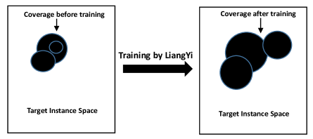
Figure 1: An intuitive example of LiangYi enlarging the coverage of the algorithm population on the target instance space. The whole target instance space is the area inside the rectangle. The $AP$ contains 3 member algorithms. The coverage of each algorithm on the target instance space is indicated by a black circle.

3.2 Implementation Details

The training module and the instance searching module in LiangYi are implemented as two evolutionary procedures $EvolveAlg$ and $EvolveIns$, respectively. In general, any search method can be used in these two procedures. In our work, evolutionary algorithms (EAs) [37] are employed as the off-the-shelf tools, because EAs are suitable for handling populations (of either algorithms or instances) and are less restricted by the properties of objective functions (in comparison to other search methods such as gradient descent that requires differentiable objective functions). The behaviors of $EvolveAlg$ and $EvolveIns$ are controlled by parameter sets $params_{AP}$ and $params_{IP}$, respectively.

When applying EAs to evolve $AP$ and $IP$, the basic aspects that need to be considered are the representation, the variation (search operators such as crossover and mutation), the evaluation and the selection of the individuals in both populations. Generally, the representation and the variation of the individuals greatly determine the search space for EA. In our work the expected search spaces for EAs are the parameter configuration space $\Theta$ and the target instance space $\Gamma$, which are actually strongly correlated to the used parameterized algorithm and the target problem class, respectively. Thus in the framework of LiangYi, we do not specify the individual representation and variation. When applying LiangYi, the design issues in these two aspects should be addressed according to the target problem class and the chosen parameterized algorithm.

Before going into the details of $EvolveAlg$ and $EvolveIns$, we explain here how to measure the performance of a population-based solver, which is the basis of the individual evaluation in both populations. Let $P(\mathrm{solver,instance\ set})$ denote the performance of a solver on an instance set according to a given performance metric $m$, in which the solver could be a single algorithm or an $AP$ and the instance set could be a single instance or an $IP$. Since a population-based solver runs all member algorithms in parallel when solving an instance, the performance of $AP$ on an instance $ins$ is the best performance achieved by its member algorithms on $ins$ (we assume a larger value is better for $m$ without loss of generality), i.e,

$$P(AP,ins)=\max_{alg\in AP}P(alg,ins).$$ (1)

The performance of $AP$ on $IP$ is an aggregated value of the performance of $AP$ on each instance of $IP$, i.e.,

$$P(AP,IP)=\underset{ins\in IP}{Aggr}(P(AP,ins))$$ (2)

where $Aggr()$ is an aggregate function. The performance metric $m$ and the aggregate function $Aggr()$ are user-specified.

3.2.1 Evolution of the Algorithm Population

The pseudo code of $EvolveAlg$ is shown in Procedure 2.

Procedure 2 $EvolveAlg(AP_{k},IP_{k},params_{AP})$

$Memory$ is a global cache storing the final $AP$ and the final performance matrix $M$ of $EvolveAlg$ in each cycle of LiangYi

0.  Algorithm population $AP_{k}$, instance population $IP_{k}$, parameter set $params_{AP}$ containing: set of parameters which control $VariationAlg$, $params_{VarA}$, and set of parameters which control $RemoveWorst$, $params_{R}$

0.  current AP when $EvolveAlg$ is terminated

1.  $M\leftarrow$ Test $AP_{k}$ on $IP_{k}$

2.  while not $EvolveAlgTermination()$ do

3.     $a_{1},a_{2}\leftarrow$ Randomly select two individuals from $AP_{k}$

4.     $a_{new}\leftarrow$ $VariationAlg(a_{1},a_{2},params_{VarA})$

5.     $M_{new}\leftarrow$ Test $a_{new}$ on $IP_{k}$

6.     $AP^{\prime}_{k}\leftarrow AP_{k}\cup\{a_{new}\}$

7.     $M^{\prime}\leftarrow$ Vertically concatenate $M$ and $M_{new}$

8.     $AP_{k},M\leftarrow RemoveWorst(AP_{k}^{\prime},M^{\prime},params_{R})$

9.  end while

10.  Add $AP_{k}$ and $M$ to $Memory$

11.  return  $AP_{k}$

First of all, $AP_{k}$ is tested on $IP_{k}$ and the result is represented by a $N_{AP}\times N_{IP}$ matrix $M$ ($N_{AP}$ and $N_{IP}$ are the number of the algorithms in $AP$ and the number of the instances in $IP$, respectively), in which each row corresponds to an algorithm in $AP_{k}$ and each column corresponds to an instance in $IP_{k}$, so each entry in $M$ is the performance of the corresponding algorithm in $AP_{k}$ on the corresponding instance in $IP_{k}$ (Line 1). Then at each generation, two individuals are randomly selected from $AP_{k}$ and an offspring is generated by variation (Lines 3-4). The generated algorithm $a_{new}$ is then tested on $IP_{k}$ and the result is represented by a $1\times N_{IP}$ matrix $M_{new}$ (Line 5). The last step is to decide the survivors of this generation (Lines 6-8). Together with all the algorithms in $AP_{k}$, $a_{new}$ is put into a temporary algorithm population $AP^{\prime}$. The corresponding performance matrix $M^{\prime}$ to $AP^{\prime}$, of which the size is $(N_{AP}+1)\times N_{IP}$, is constructed by concatenating $M$ and $M_{new}$ vertically. Then the procedure $RemoveWorst$ is run to decide which algorithm in $AP^{\prime}$ will be removed.

Basically, $RemoveWorst$ first calculates the fitness of each algorithm in $AP^{\prime}$ and then selects the algorithm with the lowest fitness to be removed. The core of $RemoveWorst$ is its fitness evaluation. The idea is that an algorithm will be preferred only if it contributes to $AP$, and the more it contributes, the more it is preferred. The contribution of a member algorithm is actually the performance improvement it brings to the population, which can be calculated as the population’s performance loss caused by removing the algorithm. Formally, let $C(AP,IP,alg)$ denote the contribution of algorithm $alg$ to the performance of $AP$ on $IP$. If $|AP|>1$, which means $AP$ contains other algorithms besides $alg$, $C(AP,IP,alg)$ is calculated via Equation (3):

$$C(AP,IP,alg)=|P(AP,IP)-P(AP-\{alg\},IP)|,$$ (3)

where $P(AP,IP)$ and $P(AP-\{alg\},IP)$ are calculated via Equation (2). If $|AP|=1$, which means $AP$ only contains one algorithm (i.e., $alg$), and then removing $alg$ from $AP$ will cause complete performance loss on $IP$. In this case, $C(AP,IP,alg)$ is calculated via Equation (4):

$$C(AP,IP,alg)=\alpha|P(AP,IP)|,$$ (4)

where the parameter $\alpha>0$.

Based on Equation (4), for each member algorithm $alg$ in the temporary algorithm population $AP_{k}^{\prime}$, its performance contribution on $IP_{k}$ is $C(AP_{k}^{\prime},IP_{k},alg)$. A high contribution indicates that the corresponding algorithm should be reserved to next generation. However, directly using $C(AP_{k}^{\prime},IP_{k},alg)$ as the fitness of $alg$ is not appropriate. As aforementioned (see Section 3.1), the evolution of $AP_{k}$ should not only improve the performance of $AP_{k}$ on $IP_{k}$, but also keep the good performances obtained in previous cycles (on $IP_{1},...,IP_{k-1}$). Using $C(AP_{k}^{\prime},IP_{k},alg)$ to evaluate $alg$ only considers the first target. Hence the fitness of $alg$ is calculated based on two types of contributions: The first one is the current performance contribution, i.e., $C(AP_{k}^{\prime},IP_{k},alg)$, and the second one is the historical performance contribution of $alg$ on $IP_{1},...,IP_{k-1}$ (if there exist).

To calculate the historical performance contribution, the concept $\mathit{age}$ is introduced to describe how long an algorithm has been in $AP$. Suppose an algorithm $alg$ in $AP_{k}^{\prime}$ was added to $AP$ in the $j$-th cycle of LiangYi (and now is in the $k$-th cycle), the $age$ of $alg$ is $k-j$. The performance of $alg$ on $IP_{j}$,…,$IP_{k}$ are known because $alg$ has been tested on them in corresponding cycles of LiangYi . To calculate the historical performance contribution of $alg$ on $IP_{r}(j\leq r\leq k-1)$, the algorithms that are in $AP_{k}^{\prime}$ and satisfy the condition $age\geq(k-r)$ are selected (our target algorithm $alg$ is also selected, since its $age$ is $k-j$, which satisfies the condition) to form a virtual algorithm population $virtualAP_{r}$. The condition $age\geq(k-r)$ indicates that these selected algorithms were added to $AP$ during or before the $r$-th cycle of LiangYi, so they have been tested on $IP_{r}$. The performances of these algorithms on $IP_{r}$ are represented by a $|virtualAP_{r}|\times N_{IP}$ matrix $virtualM_{r}$. If $|virtualAP_{r}|>1$, which means $virtualAP_{r}$ contains other algorithms besides $alg$, the performance contribution of $alg$ on $IP_{r}$ is calculated via Equation (3):

$$C(virtualAP_{r},IP_{r},alg)=|P(virtualAP_{r},IP_{r})-P(virtualAP_{r}-\{alg\},IP_{r})|.$$

If $|virtualAP_{r}|=1$ , which means $virtualAP_{r}$ only contains $alg$, and thus removing $alg$ from $virtualAP_{r}$ will cause complete loss of performance on $IP_{r}$. In this case, $C(virtualAP_{r},IP_{r},alg)$ is calculated via Equation (4):

$$C(virtualAP_{r},IP_{r},alg)=\alpha|P(virtualAP_{r},IP_{r})|.$$

Now we have all the performance contributions of $alg$ on $IP_{j}$,…,$IP_{k}$. The fitness of $alg$, denoted as $f_{AP}(alg)$, is calculated via Equation (5)

$$f_{AP}(alg)=\frac{\beta\Sigma_{j\leq r\leq k-1}{C(virtualAP_{r},IP_{r},alg)}+C(AP^{\prime}_{k},IP_{k},alg)}{k-j+1}$$ (5)

where $k$ is the index of the current cycle of $LiangYi$, $j$ is the $age$ of $alg$, and $\beta$ is a nonnegative parameter. The terms $C(virtualAP_{r},IP_{r},alg)(j\leq r\leq k-1)$ are historical performance contributions on $IP_{j}$,…,$IP_{k-1}$, while $C(AP^{\prime}_{k},IP_{k},alg)$ is the current performance contribution on $IP_{k}$. Thereby the numerator in the fraction is actually a weighted sum of $(k-j+1)$ performance contributions, in which the parameter $\beta$ is used to balance between historical performance contributions(on $IP_{1},...,IP_{k-1}$) and current performance contribution (on $IP_{k}$).

The pseudo code of $RemoveWorst$ is demonstrated in Procedure 3. First the fitness of each algorithm in $AP^{\prime}_{k}$ is calculated (Lines 1-15). Specifically, for an algorithm $alg$ which was added to $AP$ in the $j$-th cycle of LiangYi, $k-j$ virtual algorithm populations, i.e., $virtualAP_{j},...,virtualAP_{k-1}$, are constructed (according to the global cache Memory) to calculate its historical performance contributions on $IP_{j},...,IP_{k-1}$, via Equation (3) or Equation (4) (Lines 2-12). Together with the current performance contribution calculated via Equation (3) (Line 13), the historical contributions are used to calculate the fitness of $alg$ via Equation (5) (Line 14). After the fitness of each algorithm in $AP^{\prime}_{k}$ has been calculated, the algorithm with the lowest fitness will be removed (Line 16).

Procedure 3 $RemoveWorst(AP^{\prime}_{k},M^{\prime},params_{R})$

0.  Temporary algorithm population $AP^{\prime}_{k}$, temporary performance matrix $M^{\prime}$, parameter set $params_{R}$ containing $\alpha$ (used in Equation (4)) and $\beta$ (used in Equation (5))

0.  $AP_{k}$, performance matrix $M$

1.  for each algorithm $alg$ in $AP^{\prime}_{k}$ do

2.     $age\leftarrow$ Query $Memory$ for how many cycles $alg$ has been staying

3.     $j\leftarrow k-age$

4.     for $r\leftarrow j$ to $k-1$ do

5.        $VirtualAP_{r}\leftarrow$ Select algorithms which satisfy the condition $age\geq(k-r)$ (according to $Memory$) from $AP^{\prime}_{k}$

6.        $M_{r}\leftarrow$ Construct corresponding performance matrix to $VirtualAP_{r}$ (according to $Memory$)

7.        if $|virtualAP_{r}|>1$ then

8.           $C(virtualAP_{r},IP_{r},alg)\leftarrow$ Calculate the algorithm contribution of $alg$ on $IP_{r}$ via Equation (3)

9.        else

10.           $C(virtualAP_{r},IP_{r},alg)\leftarrow$ Calculate the algorithm contribution of $alg$ on $IP_{r}$ via Equation (4)

11.        end if

12.     end for

13.     $C(AP^{\prime}_{k},IP_{k},alg)\leftarrow$ Calculate the algorithm contribution of $alg$ on $IP_{k}$ via Equation (3)

14.     $f_{AP}(alg)\leftarrow$ Calculate the fitness of $alg$ via Equation (5)

15.  end for

16.  $AP_{k},M\leftarrow$ Remove the algorithm with the lowest fitness from $AP_{k}^{\prime}$ and the corresponding row from $M^{\prime}$

17.  return  $AP_{k}$, $M$

3.2.2 Evolution of the Instance Population

As aforementioned (see Section 3.1) the evolution of $IP$ aims at discovering those instances that cannot be solved well by $AP$; thus the fitness of an instance in $IP$ is measured by how $AP$ performs on it — the worse the performance, the higher the fitness.

The pseudo code of $EvolveIns$ is demonstrated in Procedure 4. First of all, $AP_{k+1}$ is tested on the $IP_{k}$ and the result is represented by a $N_{AP}\times N_{IP}$ matrix $M$ (Line 1), and the fitness of each instance is calculated (Lines 2-4). The fitness of an instance $ins$, denoted as $f_{IP}(ins)$, is calculated via Equation (6):

$$f_{IP}(ins)=-P(AP_{k+1},ins),$$ (6)

where $P(AP_{k+1},ins)$ is the performance of $AP_{k+1}$ on instance $ins$, calculated via Equation (1). At each generation, $N_{IP}*re$ new instances are generated by repeatedly selecting two instances from $IP_{k}$ (using tournament selection [37]) and creating two offsprings by variation (Lines 6-11). These offsprings are then tested against the algorithm population $AP_{k+1}$ and the fitness of each offspring is calculated (Lines 12-15). At the end of this generation, all instances in $IP_{k}$ and the offsprings are put into a candidate pool and the worst $N_{IP}*re$ instances are removed (Lines 16-19).

Procedure 4 $EvolveIns(AP_{k+1},IP_{k},params_{IP})$

0.  Algorithm population $AP_{k+1}$, instance population $IP_{k}$, parameter set $params_{IP}$ containing: set of parameters which control $VariationIns$, $params_{VarI}$, and replacement ratio $res$

0.  current $IP$ when $EvolveIns$ is terminated

1.  $M\leftarrow$ Test $AP_{k+1}$ on $IP_{k}$

2.  for each instance $ins$ in $IP_{k}$ do

3.     $f_{IP}(ins)\leftarrow$ Calculate the fitness of $ins$ via Equation (6)

4.  end for

5.  while not $EvolveInsTermination()$ do

6.     $offsprings\leftarrow\varnothing$

7.     for $i\leftarrow 1$ to $\frac{N_{IP}*res}{2}$ do

8.        $ins_{1},ins_{2}\leftarrow$ Select two parents from $IP_{k}$ with tournament selection

9.        $ins_{new1},ins_{new2}\leftarrow VariationIns(ins_{1},ins_{2},params_{VarI})$

10.        $offsprings\leftarrow offsprings\cup\{ins_{new1},ins_{new2}\}$

11.     end for

12.     $M_{offsprings}\leftarrow$ Test $AP_{k+1}$ on $offsprings$

13.     for each instance $ins$ in $offsprings$ do

14.        $f_{IP}(ins)\leftarrow$ Calculate the fitness of $ins$ via Equation (6)

15.     end for

16.     $candidates\leftarrow IP_{k}\cup offsprings$

17.     $M_{candidates}\leftarrow$ Horizontally concatenate $M$ and $M_{offspring}$

18.     $IP_{k},M\leftarrow$ Remove the worst $N_{IP}*re$ instances from $candidates$ and the corresponding columns from $M_{candidates}$

19.  end while

20.  return  $IP_{k}$

4 Case Study: the Travelling Salesman Problem

The main purpose of this section is to empirically verify whether LiangYi is an effective method for improving solvers. We evaluated LiangYi on the Travelling Salesman Problem (TSP) [38], one of the most well-known computationally hard optimization problem. Specifically, the symmetric TSP, i.e., the distance between two cities is the same in each opposite direction, with Euclidean distances in a two-dimensional space is considered here. In the remainder of this section, we first give the target scenario (including the target instances and the performance metric) where LiangYi is applied, and then instantiates LiangYi for the scenario. After that, we first compare LiangYi to other existing training methods, and then we investigate the properties of LiangYi to see whether it is able to perform as expected.

All of our experiments were carried out on a workstation of two Xeon CPU with 24 cores and 48 threads at 2.50GHz, running Ubuntu Linux 16.04.

4.1 Target Scenario

The target instances considered here are all TSP instances with problem size equal to 500, i.e., the number of cities equals to 500. This work focuses on optimizing the solver’s applicability on the target instances, i.e., the performance metric is applicability. A solver is said to be applicable to an instance if it can find a good enough solution to this instance within a given time. For TSP, the goodness of a solution $sol$ is measured by the percentage by which the tour length of $sol$ exceeds the tour length of the optimum $sol^{\star}$ , abbreviated as PEO(percentage excess optimum):

$$PEO=\frac{lengh(sol)-lengh(sol^{\star})}{lengh(sol^{\star})}*100\%.$$

With the definition of PEO, given a cut-off time $t$, a solver is said to be applicable to an instance $ins$ if the $PEO$ of the best solution found by the solver in time $t$ is below a threshold $\theta$. With the definition of the applicability of a solver to a single instance, the applicability of a solver to an instance set is defined as the fraction of the instances to which the solver is applicable.

In this paper very radical values for the cut-off time $t$ and the PEO threshold $\theta$ are adopted ($t=0.1s$ and $\theta=0.05\%$) to see whether LiangYi is able to evolve solvers that can work well under such harsh conditions.

4.2 Instantiation of LiangYi and Its Computational Cost

In order to instantiate LiangYi for the above scenario, there are several issues to be addressed. The first issue is to specify the performance function $P(\mathrm{solver},\mathrm{instance\ set})$ used by LiangYi (see Section 3.2) so that LiangYi can optimize the applicability appropriately. The performance of an algorithm $alg$ on an instance $ins$, i.e., $P(alg,ins)$ in Equation (1), is specified as follow:

$$P(alg,ins)=\begin{cases}1,\ \ \mathrm{if}\ alg\ \mathrm{is}\ \mathrm{applicable}\ \mathrm{to}\ ins\\ 0,\ \ otherwise.\end{cases}$$

Intuitively, an $AP$ is said to be applicable to an instance $ins$ if any algorithm of $AP$ is applicable to $ins$. With $P(alg,ins)$ specified as above, this definition is equivalent to the definition given by Equation (1), namely, $AP$ is applicable to $ins$ if the best algorithm of $AP$ is applicable to $ins$. The aggregate function $aggr()$ in Equation (2) is specified as returning the mean value of the aggregated terms:

$$P(AP,IP)=\frac{\sum_{ins\in IP}P(AP,ins)}{|IP|},$$

which essentially calculates the proportion of the instances to which $AP$ is applicable.

Table 2: The parameters of the CLK used

Parameters	Parameter Type	# of Candidate Values
Initialization Strategy	Categorical	4
Perturbation Strategy	Categorical	4
Search Depth	Numerical	6
Search Width	Numerical	8
Backtrack Strategy	Categorical	14

The second issue is to choose a parameterized algorithm for LiangYi to build an $AP$ based on it. The choice of the parameterized algorithm in this work is Chained Lin-Kernighan (CLK) [40]. It is a variant of the Lin-Kernighan heuristic [41], one of the best heuristics for solving symmetric TSP. CLK chains multiple runs of the Lin-Kernighan algorithm to introduce more robustness in the resulting tour. Each run starts with a perturbed version of the final tour of the previous run. We extended the original implementation of CLK to allow a more comprehensive control of its components. The parameters of the resulting algorithm are summarized in Table 2. To handle the randomness of CLK, we adopt a simple way - fixing the random seed of CLK and turning it into a deterministic algorithm. To use CLK in the target scenario (see Section 4.1), in our experiments we always set the runtime of CLK to 0.1s, and after it was terminated we checked whether PEO of the solution found was below 0.05%.

The third issue is to specify the representation and the variation of individuals in both populations (see Section 3.2). Each algorithm in $AP$ is represented by a list containing 5 integers, each of which indicates its value for the corresponding parameter. Each instance in $IP$ is represented by a list of 500 $(x,y)$ coordinates on a $10^{6}\times 10^{6}$ grids. The random initialization for $AP$ and $IP$ works by uniformly randomly selecting a value (i.e., a parameter value for the algorithm, or two coordinates for the instance) from candidate values for each entry of the individual (the algorithm or the instance). Both the variation for the individuals in $AP$ and the variation for the individuals in $IP$ are implemented as a uniform crossover and a uniform mutation [37]. The uniform crossover operates with a probability, by choosing for each entry of the offspring with equal probability either the value of the entry from the first or the second parent. The probability of the uniform crossover being operated, i.e., crossover probability, is controlled by parameters $cro_{alg}$ (in $AP$) and $cro_{ins}$ (in $IP$). The mutation consists of replacing the value of each entry of the offspring, with a probability (mutation rate), with uniformly randomly chosen one from the candidate values. The mutation rate is controlled by parameters $mu_{alg}$ (in $AP$) and $mu_{ins}$ (in $IP$).

Table 3: The parameter settings of the instantiation of LiangYi for TSP

$EvolveAlg$	$EvolveIns$
$N_{AP}=6$	$N_{IP}=150$
# of Gens = 500	# of Gens = 10
$cro_{alg}=0.6$	$cro_{ins}=1$
$mu_{alg}=0.6$	$mu_{ins}=0.8$
$\alpha=2$	$res=0.3$
$\beta=2$

The last issue is to set the termination conditions and the parameters of LiangYi. The termination condition for LiangYi is the number of cycles reaching 3. In each cycle, procedure $EvolveAlg$ will be run for 500 generations and $EvolveIns$ will be run for 10 generations. The number of algorithms in $AP$, i.e., $N_{AP}$, is set to 6, and the number of instances in $IP$, i.e., $N_{IP}$, is set to 150. The parameter settings of LiangYi are listed in Table 3. In order to maintain a high level of diversity within $AP$, the mutation rate in $evolvealg$ is set to a high value (0.4). For $evolveins$, it is important to keep the instance population exploring the target instance space instead of stagnating in some local areas, and therefore the mutation rate in $evolveins$ is also set to a high value (0.7).

We applied the instantiation of LiangYi described above to the considered scenario. The training process in which $AP$ and $IP$ are evolved alternatively is depicted in Figure 2. The computational cost of LiangYi is mainly composed of two parts: The first part is the overhead for the algorithm runs used to evaluate algorithms (in $EvolveAlg$) or instances (in $EvolveIns$); The second part is the overhead for solving exactly the instances to obtain their optima (in $EvolveIns$). For each cycle of $LiangYi$, in $EvolveAlg$ there are $(N_{AP}+AP_{G})*N_{IP}$ algorithm runs, and in $EvolveIns$ there are $(N_{IP}+IP_{G}*N_{IP}*res)*N_{AP}$ algorithm runs ($AP_{G}$ and $IP_{G}$ are the number of generations of $EvolveAlg$ and $EvolveIns$, respectively) and meanwhile there are $(N_{IP}+IP_{G}*N_{IP}*res)$ instances to be solved exactly. In our experiments, the time for each algorithm run was set to 0.1s (see Section 4.1), and the average time for exactly solving an instance was 32 seconds (specific time varied from 1 second to 15 minutes). Thus the estimated CPU time for one run of the instantiation of LiangYi was 81450 seconds (i.e., 22.6 hours).

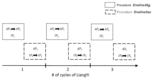
Figure 2: The training process of LiangYi in which AP and IP are evolved alternatively. Dotted rectangle and dashed rectangle represent procedure $EvolveAlg$ and procedure $EvolveIns$, respectively.

4.3 Comparative Study

In this section we compare LiangYi with other existing training methods in the considered scenario. Since the $AP$ built by LiangYi is actually a parallel portfolio, we chose ParHydra [34] (see Section 2.3) , the state-of-the-art automatic parallel portfolio construction method, as the method to compare with.

4.3.1 Settings of ParHydra

ParHydra accepts a parameterized algorithm, a set of training instances, and a performance metric to be optimized. For the target scenario considered, the performance metric is applicability. The parameterized algorithm fed to ParHydra is CLK, same as LiangYi. We used two different ways to construct the training sets for ParHydra. The first training set $IP_{random}$ was built according to the usual practice for two-stage methods — randomly generating a set of instances. Specifically, each instance in $IP_{random}$ was generated by randomly choosing two coordinates for each city on a $10^{6}\times 10^{6}$ grids. The second training set $IP_{training}$ was built by collecting the instance populations which were produced by LiangYi and once served as the training instances during the training process, i.e., $IP_{training}=IP_{1}\cup IP_{2}\cup IP_{3}$. Since LiangYi produces instance populations as by-products, it is interesting to see how good these instance populations are as training instances for existing methods like ParHydra. Both sets contain $450$ instances. The solvers output by ParHydra based on $IP_{random}$ and $IP_{training}$ are denoted as $PH_{random}$ and $PH_{LiangYi}$, respectively.

ParHydra is an iterative method, which builds the portfolio from scratch and adds an algorithm to it in each iteration (See Section 2.3). Thus we set the iteration number of ParHydra to 6 to keep in line with LiangYi in terms of algorithm number. ParHydra iteratively calls an algorithm configurator as a subroutine. In our experiments we used ParamILS [6] (version 2.3.8 with its default instantiation of FocusedILS with adaptive capping). Since the implementation of ParamILS does not provide an option to directly optimize applicability, we set the metric used in ParamILS to penalized average runtime, PAR1000 , in our setting which is equivalent to optimizing applicability. At each iteration of ParHydra, 15 copies of ParamILS [6] were run with different random seeds in parallel to obtain 15 candidate algorithms, and the one achieving the best performance on the training set was added to the portfolio. The termination condition for each ParamILS run was the total run time for configured algorithm (CLK) reaching 5 hours. Thus the estimated total computation cost for a run of ParHydra was 450 CPU hours (32.14 days).

4.3.2 Experimental Protocol

Since LiangYi and ParHydra are both stochastic methods, we ran each comparative method 20 times and compare their test results. Specifically, first we ran LiangYi 20 times, and therefore we obtained 20 $IP_{training}$ from these runs. Then we randomly generated 20 different $IP_{random}$, and based on each of these 40 training set (including $IP_{random}$ and $IP_{training}$), we ran ParHydra to obtain a solver. The random seeds used in the training processes of $PH_{random}$ are the same as the ones used in the training processes of $PH_{random}$. Finally in total we obtained 20 $AP_{4}$ (the $AP$ output by LiangYi), 20 $PH_{random}$ and 20 $PH_{LiangYi}$. In order to adequately assess the performances of these output solvers in the target scenario, we generated a huge test set, denoted as $IP_{test}$, containing 10000 TSP instances with the number of cities equal to 500. Specifically, each instance was generated by randomly choosing two coordinates for each city from the interval $[0,10^{6})$. To our knowledge, this is the first time that a test set of such a large size (10000) is used to test TSP solvers.

The runtime requirements in CPU days were as follows: 18.9 days for LiangYi training (including 20 runs); 642.8 days for ParHydra training (including 20 runs); 7.80 days for testing (including the time for obtaining the optima of the test instances).

4.3.3 Experiment Results

The average test results of these three types of solvers (with each type containing 20 solvers) are presented in Table 4. Since for each $AP_{4}$ there is a $PH_{LiangYi}$ that shares the training instances with it, we performed a two-sided Wilcoxon signed-rank test to check whether the difference between the results obtained by $AP_{4}$ and $PH_{LiangYi}$ are statistically significant. We also performed a two-sided Wilcoxon signed-rank test for $PH_{random}$ and $PH_{LiangYi}$, since they share the common random seeds. For $AP_{4}$ and $PH_{random}$, we performed a two-sided Wilcoxon rank-sum test. All the tests were carried out with a 0.05 significance level. The statistical test results are also presented in Table 4. $PH_{LiangYi}$ obtained better results than $PH_{random}$, indicating the training instances produced by LiangYi are more representative of the target scenario than the randomly generated ones. It is a little surprising to see $AP_{4}$ obtained better results than $PH_{LiangYi}$ at the first sight. Different from $AP_{4}$, $PH_{LiangYi}$ was directly trained with the whole $IP_{training}$, which was produced by LiangYi cycle by cycle; thus it is conceivable that $PH_{LiangYi}$ would obtain better results on $IP_{training}$ than $AP_{4}$ (actually their performances on $IP_{training}$, i.e., $P(AP_{4},IP_{training})$ and $P(PH_{LiangYi},IP_{training})$, are 0.6063 and 0.6644). The reason why $AP_{4}$ obtained better results than $PH_{LiangYi}$ on $IP_{test}$ is as follow: The adaptive instance updating strategy used by LiangYi can be seen as a filter that only reserves those hard instances for $AP$ to make the training focus on them, which makes the actual coverage of $AP$ on the target instances far greater than its coverage on $IP_{training}$ ($0.7001>0.6063$), because those easy target instances which are sampled by $EvolveIns$ and are actually covered by $AP$ are all filtered out. Compared to LiangYi, ParHydra accepts all the training instances and only focuses on the training set. The lack of the instance adaptability makes the performance of the output solver greatly depend on how much the training set can represent the target scenario.

In Table 5, we also give the average PEO (see Section 4.1) obtained by the three types of solvers on $IP_{test}$. $AP_{4}$ is still significantly better than $PH_{LiangYi}$ and $PH_{random}$. Although in the target scenario we actually did not directly optimize the solution quality, LiangYi managed to evolve solvers that on average satisfy the PEO requirements in the scenario (0.05%).

Table 4: Test result comparisons of $AP_{4},PH_{random}$ and $PH_{LiangYi}$. The test results are presented in terms of applicability, i.e., the proportion of the instances to which the solver is applicable. We performed statistical tests to compare their results, considering p-values below 0.05 to be statistically significant. The last two columns provide the results of the test, where ${}^{\prime}W^{\prime}$, ${}^{\prime}D^{\prime}$, and ${}^{\prime}L^{\prime}$ indicate the corresponding solver is superior to, not significantly different from or inferior to the competitor, respectively.

	Average test results (applicability)	Statistical test results
		vs.$PH_{LiangYi}$	vs.$PH_{random}$
$AP_{4}$	$0.6822\pm 0.0082$	W	W
$PH_{LiangYi}$	$0.6383\pm 0.0138$	$\boldsymbol{-}$	W
$PH_{random}$	$0.6290\pm 0.0133$	L	$\boldsymbol{-}$

Table 5: Average PEO (see Section 4.1) comparisons of $AP_{4},PH_{random},PH_{LiangYi}$ on $IP_{test}$. We performed statistical tests here similar to the ones in the comparisons of average test results (applicability).

	Average PEO	Statistical test results
		vs.$PH_{LiangYi}$	vs.$PH_{random}$
$AP_{4}$	$0.0497\%\pm 0.0010\%$	W	W
$PH_{LiangYi}$	$0.0532\%\pm 0.0018\%$	$\boldsymbol{-}$	D
$PH_{random}$	$0.0539\%\pm 0.0015\%$	D	$\boldsymbol{-}$

4.4 Investigating the Properties of LiangYi

As aforementioned, the idea behind LiangYi is to optimize the performance of $AP$ on target instances by a) improving its performance on those instances on which it performs badly and b) keeping its good performance on those instances on which it performs well. The main purpose of this section is to investigate whether LiangYi is able to accomplish the two objectives listed above. Specifically, the verification is divided into two parts — the training part and the test part. In the training part we investigate that, in the training process, whether LiangYi gives satisfactory answers to the following three questions:

1. Is procedure $evolvealg$ able to improve the performance of $AP$ on current $IP$?

2. Is procedure $evolveins$ able to degrade the performance of $AP$ on current $IP$?

3. Is procedure $evolvealg$ able to keep the performance of $AP$ on previous $IPs$?

The second question indicates whether the evolution of $IP$ is able to discover and include hard-to-solve instances to $AP$, and the first question indicates whether the evolution of $AP$ is able to improve the performance of $AP$ on the hard instances included in the current $IP$. The combination of these two checks the whether LiangYi is able to accomplish the first objective. The third question checks whether LiangYi is able to accomplish the second objective. In addition to focusing on the three specific aspects, we also directly check if LiangYi is able to continuously improve $AP$ in the training part. Specifically, we check whether the performance of $AP$ on $IP_{training}$ that are produced in the training are improved by LiangYi. Similarly, in the test part we also directly check whether the performance of $AP$ at the optimization task is being improved by LiangYi.

4.4.1 Training Part

To answer the first question and the second question, the performance of $AP$ on $IP$ during the training process averaged over 20 runs are plotted in Figure 3. The results depicted in Figure 3 clearly show that, at each cycle of LiangYi, $EvolveAlg$ improves the performance of $AP_{k}$ on $IP_{k}$, and $evolveins$ degrades the performance of $AP_{k+1}$ on $IP_{k}$, which gives positive answers to the first two questions, thus confirming the first aspect of the idea behind LiangYi.

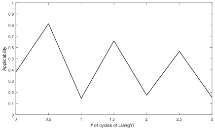
Figure 3: The performance of $AP$ on $IP$ at the beginning ($EvolveAlg$ begins), the middle ($EvolveAlg$ ends) and the end ($EvolveIns$ ends) of each cycle of LiangYi. The performances are represented in terms of applicability, i.e., the proportion of the instances to which AP is applicable, and are averaged over 20 runs.

The third question is answered in this way: Since procedure $evolvealg$ evolved $AP_{k}$ to $AP_{k+1}$ to improve the performance on $IP_{k}$, we checked whether the improvement from $P(AP_{k},IP_{k})$ to $P(AP_{k+1},IP_{k})$, i.e., $|P(AP_{k},IP_{k})-P(AP_{k+1},IP_{k})|$, was kept in subsequent cycles of LiangYi. Specifically, we tested $AP_{k+2},...,AP_{4}$ on $IP_{k}$ to obtain their performances on $IP_{k}$, i.e., $P(AP_{k+2},IP_{k}),...,P(A_{4},IP_{k})$, and calculated the performance drops from $P(AP_{k+1},IP_{k})$ to these performances, i.e., $|P(AP_{k+1},IP_{k})-P(AP_{k+2},IP_{k})|$,…, $|P(AP_{k+1},IP_{k})-P(A_{4},IP_{k})|$, then these performance drops were compared to the performance improvement. The averaged performances (over 20 runs) of $AP_{k},...,AP_{4}$ on $IP_{k}$ are presented in Table 6. The average performance improvement on $IP_{1}$ is $P(AP_{2},IP_{1})-P(AP_{1},IP_{1})=0.4321$, and the two average performance drops on $IP_{1}$ are $P(AP_{3},IP_{1})-P(AP_{2},IP_{1})=0.0700$ and $P(AP_{4},IP_{1})-P(AP_{2},IP_{1})=0.1254$, so the ratios between the performance drops and the performance improvements on $IP_{1}$ are 16.20% and 29.02%. Calculated in the same way, the ratio on $IP_{2}$ is 17.98%. All the ratios between the performance drops and the corresponding performance improvements are below $30\%$.

Table 6: Performances of $AP_{k}$,…$AP_{4}$ on $IP_{k}$. All the results are presented in terms of applicability, i.e., the proportion of the instances to which $AP$ is applicable, and are averaged over 20 runs.

	$IP_{1}$	$IP_{2}$	$IP_{3}$
$AP_{1}$	0.3800
$AP_{2}$	0.8121	0.1456
$AP_{3}$	0.7421	0.6590	0.1735
$AP_{4}$	0.6867	0.5667	0.5654

In order to check whether the performances of $AP$ on $IP_{training}$ are improved by LiangYi, the algorithm populations obtained from each cycle of LiangYi, i.e., $AP_{1},AP_{2},AP_{3},AP_{4}$, were tested on $IP_{training}$. The test results averaged over 20 runs are depicted in Figure 4. A constant improvement of the performances of $AP_{k}$ on $IP_{training}$, according to the increase of $k$, is shown.

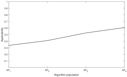
Figure 4: The performances of $AP_{1},AP_{2},AP_{3},AP_{4}$ on $IP_{training}$. The performances are represented in terms of applicability, i.e., the proportion of the instances to which AP is applicable, and are averaged over 20 runs.

4.4.2 Test Part

The algorithm population obtained from each cycle of LiangYi, i.e., $AP_{1},...,AP_{4}$ was tested on $IP_{test}$. The test results averaged over 20 runs are depicted in Figure 5. Once again, a constant improvement of the performances of $AP_{k}$ on $IP_{test}$ according to the increase of $k$ is shown.

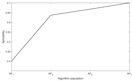
Figure 5: The performances of $AP_{1},AP_{2},AP_{3},AP_{4}$ on $IP_{test}$. The performances are represented in terms of applicability, i.e., the proportion of the instances to which AP is applicable, and are averaged over 20 runs.

5 Conclusion and Future Directions

This paper first put forward the concept of experience-based optimization (EBO) which concerns improving solvers based on their past solving experience, and summarized several previous research in a unified context, i.e., offline training of EBO. A new coevolutionary training method, dubbed LiangYi, was proposed. The most novel feature of LiangYi is that, different from existing methods, it addresses selecting training instances and training solvers simultaneously. A specific instantiation of LiangYi on TSPs was also proposed. Empirical results showed the advantages of LiangYi in comparison to ParHydra, the state-of-the-art $APC$ method, on a huge test set containing 10000 instances. Moreover, through empirically investigating behaviours of LiangYi, we confirmed that LiangYi is able to continuously improve the solver through training.

As discussed in the introduction, EBO is a far more broad direction than merely offline training of problem solvers. Further investigations may include:

1. Further improvements to LiangYi. Diversity preservation scheme, such as speciation [42] or negatively correlated search [15] can be introduced into LiangYi to explicitly promote cooperation between different algorithms in $AP$. Another tack is to use machine learning techniques to accelerate LiangYi. Specifically, regression models and classification models can be used to predict the performance of algorithms in $AP$ or instances in $IP$, without actually evaluating them, which is very time-consuming.

2. Online mode of EBO. Situations in which a solver faces a series of different problem instances coming sequentially pose new challenges. For example, the objective in online mode is to maximize the cumulative performance on all the instances. Thus methods designed for this scenario must consider making solvers perform well on current instances and improving solvers for future instances simultaneously. Besides, in a dynamic environment, the underlying properties of instances may change overtime; therefore the solvers need to keep detecting the changes of environment and adapt to new instances.

3. Deeper understanding of the fundamental issues of EBO is also worthy of exploration. For example, LiangYi actually maintains two adversary sets competing against one another, which is a typical scenario where the game theory can be applied. Besides, other more general issues in EBO include the similarity measure between instances, a unified approach to information extraction from solved instances, and theoretical proofs of the usefulness of transmitting information between similar instances.

6 Acknowledgements

This work was supported in part by the National Natural Science Foundation of China under Grant 61329302 and Grant 61672478; EPSRC under Grant EP/K001523/1 and EP/J017515/1, the Royal Society Newton Advanced Fellowship under Grant NA150123, and SUSTech. Xin Yao was also supported by a Royal Society Wolfson Research Merit Award.

References

References

- [1] C. H. Papadimitriou, K. Steiglitz, Combinatorial optimization: algorithms and complexity, Courier Corporation, 1982.
- [2] H. H. Hoos, Automated algorithm configuration and parameter tuning, in: Autonomous search, Springer, 2011, pp. 37–71.
- [3] J. A. Boyan, A. W. Moore, Learning evaluation functions to improve optimization by local search, Journal of Machine Learning Research 1 (2000) 77–112.
- [4] L. Feng, Y.-S. Ong, M.-H. Lim, I. W. Tsang, Memetic search with interdomain learning: a realization between cvrp and carp, IEEE Transactions on Evolutionary Computation 19 (5) (2015) 644–658.
- [5] R. Santana, A. Mendiburu, J. A. Lozano, Structural transfer using edas: An application to multi-marker tagging snp selection, in: 2012 IEEE Congress on Evolutionary Computation, IEEE, 2012, pp. 1–8.
- [6] F. Hutter, H. H. Hoos, K. Leyton-Brown, T. Stützle, Paramils: an automatic algorithm configuration framework, Journal of Artificial Intelligence Research 36 (1) (2009) 267–306.
- [7] J. R. Rice, The algorithm selection problem, Advances in computers 15 (1976) 65–118.
- [8] K. A. Smith-Miles, Cross-disciplinary perspectives on meta-learning for algorithm selection, ACM Computing Surveys (CSUR) 41 (1) (2009) 6.
- [9] L. Kotthoff, Algorithm selection for combinatorial search problems: A survey, AI Magazine 35 (3) (2014) 48–60.
- [10] L. Xu, H. Hoos, K. Leyton-Brown, Hydra: Automatically configuring algorithms for portfolio-based selection., in: AAAI, Vol. 10, 2010, pp. 210–216.
- [11] L. Xu, F. Hutter, H. H. Hoos, K. Leyton-Brown, Hydra-mip: Automated algorithm configuration and selection for mixed integer programming, in: RCRA workshop on experimental evaluation of algorithms for solving problems with combinatorial explosion at the international joint conference on artificial intelligence (IJCAI), 2011, pp. 16–30.
- [12] S. Kadioglu, Y. Malitsky, M. Sellmann, K. Tierney, Isac-instance-specific algorithm configuration., in: ECAI, Vol. 215, 2010, pp. 751–756.
- [13] Y. Malitsky, M. Sellmann, Instance-specific algorithm configuration as a method for non-model-based portfolio generation, in: International Conference on Integration of Artificial Intelligence (AI) and Operations Research (OR) Techniques in Constraint Programming, Springer, 2012, pp. 244–259.
- [14] K. Tang, F. Peng, G. Chen, X. Yao, Population-based algorithm portfolios with automated constituent algorithms selection, Information Sciences 279 (2014) 94–104.
- [15] K. Tang, P. Yang, X. Yao, Negatively correlated search, IEEE Journal on Selected Areas in Communications 34 (3) (2016) 542–550.
- [16] T. M. Mitchell, Machine learning. 1997, Burr Ridge, IL: McGraw Hill 45 (1997) 37.
- [17] B. Adenso-Diaz, M. Laguna, Fine-tuning of algorithms using fractional experimental designs and local search, Operations Research 54 (1) (2006) 99–114.
- [18] C. Ansótegui, M. Sellmann, K. Tierney, A gender-based genetic algorithm for the automatic configuration of algorithms, in: International Conference on Principles and Practice of Constraint Programming, Springer, 2009, pp. 142–157.
- [19] F. Hutter, H. H. Hoos, K. Leyton-Brown, Sequential model-based optimization for general algorithm configuration, in: International Conference on Learning and Intelligent Optimization, Springer, 2011, pp. 507–523.
- [20] M. López-Ibánez, J. Dubois-Lacoste, T. Stützle, M. Birattari, The irace package, iterated race for automatic algorithm configuration, Tech. rep., Citeseer (2011).
- [21] J. N. Hooker, Testing heuristics: We have it all wrong, Journal of heuristics 1 (1) (1995) 33–42.
- [22] K. Smith-Miles, S. Bowly, Generating new test instances by evolving in instance space, Computers & Operations Research 63 (2015) 102–113.
- [23] L. Xu, F. Hutter, H. H. Hoos, K. Leyton-Brown, Satzilla: portfolio-based algorithm selection for sat, Journal of Artificial Intelligence Research 32 (2008) 565–606.
- [24] M. Gebser, R. Kaminski, B. Kaufmann, T. Schaub, M. T. Schneider, S. Ziller, A portfolio solver for answer set programming: Preliminary report, in: International Conference on Logic Programming and Nonmonotonic Reasoning, Springer, 2011, pp. 352–357.
- [25] K. Leyton-Brown, E. Nudelman, Y. Shoham, Empirical hardness models: Methodology and a case study on combinatorial auctions, Journal of the ACM (JACM) 56 (4) (2009) 22.
- [26] F. Hutter, L. Xu, H. H. Hoos, K. Leyton-Brown, Algorithm runtime prediction: Methods & evaluation, Artificial Intelligence 206 (2014) 79–111.
- [27] H. Hoos, M. Lindauer, T. Schaub, claspfolio 2: Advances in algorithm selection for answer set programming, Theory and Practice of Logic Programming 14 (4-5) (2014) 569–585.
- [28] M. Lindauer, H. H. Hoos, F. Hutter, T. Schaub, Autofolio: an automatically configured algorithm selector, Journal of Artificial Intelligence Research 53 (2015) 745–778.
- [29] L. Xu, F. Hutter, J. Shen, H. H. Hoos, K. Leyton-Brown, Satzilla2012: Improved algorithm selection based on cost-sensitive classification models, Proceedings of SAT Challenge (2012) 57–58.
- [30] S. Kadioglu, Y. Malitsky, A. Sabharwal, H. Samulowitz, M. Sellmann, Algorithm selection and scheduling, in: International Conference on Principles and Practice of Constraint Programming, Springer, 2011, pp. 454–469.
- [31] Y. Malitsky, A. Sabharwal, H. Samulowitz, M. Sellmann, Boosting sequential solver portfolios: Knowledge sharing and accuracy prediction, in: International Conference on Learning and Intelligent Optimization, Springer, 2013, pp. 153–167.
- [32] Y. Malitsky, A. Sabharwal, H. Samulowitz, M. Sellmann, Algorithm portfolios based on cost-sensitive hierarchical clustering., in: IJCAI, 2013.
- [33] L. Kotthoff, I. P. Gent, I. Miguel, An evaluation of machine learning in algorithm selection for search problems, AI Communications 25 (3) (2012) 257–270.
- [34] M. Lindauer, H. Hoos, K. Leyton-Brown, T. Schaub, Automatic construction of parallel portfolios via algorithm configuration, Artificial Intelligence.
- [35] W. D. Hillis, Co-evolving parasites improve simulated evolution as an optimization procedure, Physica D: Nonlinear Phenomena 42 (1-3) (1990) 228–234.
- [36] F. Peng, K. Tang, G. Chen, X. Yao, Population-based algorithm portfolios for numerical optimization, IEEE Transactions on Evolutionary Computation 14 (5) (2010) 782–800.
- [37] T. Back, Evolutionary algorithms in theory and practice: evolution strategies, evolutionary programming, genetic algorithms, Oxford university press, 1996.
- [38] E. L. Lawler, J. K. Lenstra, A.-G. Rinnooy-Kan, D. B. Shmoys, traveling salesman problem.[the].
- [39] D. Applegate, R. Bixby, V. Chvatal, W. Cook, Concorde tsp solver (2006).
- [40] D. Applegate, W. Cook, A. Rohe, Chained lin-kernighan for large traveling salesman problems, INFORMS Journal on Computing 15 (1) (2003) 82–92.
- [41] S. Lin, B. W. Kernighan, An effective heuristic algorithm for the traveling-salesman problem, Operations research 21 (2) (1973) 498–516.
- [42] M. Črepinšek, S.-H. Liu, M. Mernik, Exploration and exploitation in evolutionary algorithms: A survey, ACM Computing Surveys (CSUR) 45 (3) (2013) 35.