Inverse Risk-Sensitive Reinforcement Learning

Abstract

We address the problem of inverse reinforcement learning in Markov decision processes where the agent is risk-sensitive. We derive a risk-sensitive reinforcement learning algorithm with convergence guarantees that employs convex risk metrics and models of human decision-making deriving from behavioral economics. The risk-sensitive reinforcement learning algorithm provides the theoretical underpinning for a gradient-based inverse reinforcement learning algorithm that minimizes a loss function defined on observed behavior of a risk-sensitive agent. We demonstrate the performance of the proposed technique on two examples: (i) the canonical Grid World example and (ii) a Markov decision process modeling ride-sharing passengers’ decisions given price changes. In the latter, we use pricing and travel time data from a ride-sharing company to construct the transition probabilities and rewards of the Markov decision process.

I Introduction

The modeling and learning of human decision-making behavior is increasingly becoming important as critical systems begin to rely more on automation and artificial intelligence. Yet, in this task we face a number of challenges, not least of which is the fact that humans are known to behave in ways that are not completely rational. There is mounting evidence to support the fact that humans often use reference points—e.g., the status quo or former experiences or recent expectaions about the future that are otherwise perceived to be related to the decision the human is making [1, 2]. It has also been observed that their decisions are impacted by their perception of the external world (exogenous factors) and their present state of mind (endogenous factors) as well as how the decision is framed or presented [3].

The success of descriptive behavioral models in capturing human behavior has long been touted by the psychology community and, more recently, by the economics community. In the engineering context, humans have largely been modeled, under rationality assumptions, from the so-called normative point of view where things are modeled as they ought to be, which is counter to a descriptive as is point of view.

However, risk-sensitivity in the context of learning to control stochastic dynamical systems (see, e.g., [4, 5]) has been fairly extensively explored in engineering. Many of these approaches are targeted at mitigating risks due to uncertainties in controlling a system such as a plant or robot where risk-aversion is captured by leveraging techniques such as exponential utility functions or minimizing mean-variance criteria.

Complex risk-sensitive behavior arising from human interaction with automation is only recently coming into focus. Human decision makers can be at once risk-averse and risk-seeking depending their frame of reference. The adoption of diverse behavioral models in engineering—in particular, in learning and control—is growing due to the fact that humans are increasingly playing an integral role in automation both at the individual and societal scale. Learning accurate models of human decision-making is important for both prediction and description. For example, control/incentive schemes need to predict human behavior as a function of external stimuli including not only potential disturbances but also the control/incentive mechanism itself. On the other hand, policy makers and regulatory agencies, e.g., are interested in interpreting human reactions to implemented regulations and policies.

Approaches for integrating the risk-sensitivity in the control and reinforcement learning problems via behavioral models have recently emerged [6, 7, 8, 9, 10]. These approaches largely assume a risk-sensitive Markov decision process (MDP) formulated based on a model that captures behavioral aspects of the human’s decision-making process. We refer the problem of learning the optimal policy in this setting as the forward problem. Our primary interest is in solving the so-called inverse problem which seeks to estimate the decision-making process given a set of demonstrations; yet, to do so requires a well formulated forward problem with convergence guarantees.

Inverse reinforcement learning in the context of recovering policies directly (or indirectly via first learning a representation for the reward) has long been studied in the context expected utility maximization and MDPs [11, 12, 13]. We may care about, e.g., producing the value and reward functions (or at least, characterize the space of these functions) that produce behaviors matching that which is observed. On the other hand, we may want to extract the optimal policy from a set of demonstrations so that we can reproduce the behavior in support of, e.g., designing incentives or control policies. In this paper, our focus is on the combination of these two tasks.

We model human decision-makers as risk-sensitive Q-learning agents where we exploit very rich behavioral models from behavioral psychology and economics that capture a whole spectrum of risk-sensitive behaviors and loss aversion. We first derive a reinforcement learning algorithm that leverages convex risk metrics and behavioral value functions. We provide convergence guarantees via a contraction mapping argument. In comparison to previous work in this area [14], we show that the behavioral value functions we introduce satisfy the assumptions of our theorems.

Given the forward risk-sensitive reinforcement learning algorithm, we propose a gradient-based learning algorithm for inferring the decision-making model parameters from demonstrations—that is, we propose a framework for solving the inverse risk-sensitive reinforcement learning problem with theoretical guarantees. We show that the gradient of the loss function with respect to the model parameters is well-defined and computable via a contraction map argument. We demonstrate the efficacy of the learning scheme on the canonical Grid World example and a passenger’s view of ride-sharing modeled as an MDP with parameters estimated from real-world data.

The work in this paper significantly extends our previous work [15] first, by providing the proofs for the theoretical results appearing in the earlier work and second, by providing a more extensive theory for both the forward and inverse risk-sensitive reinforcement problems.

The remainder of this paper is organized as follows. In Section II, we overview the model we assume for risk-sensitive agents, show that it is amenable to integration with the behavioral models, and present our risk-sensitive Q-learning convergence results. In Section III, we formulate the inverse reinforcement learning problem and propose a gradient–based algorithm to solve it. Examples that demonstrate the ability of the proposed scheme to capture a wide breadth of risk-sensitive behaviors are provided in Section IV. We comment on connections to recent related work in Section V. Finally, we conclude with some discussion in Section VI.

II Risk-Sensitive Reinforcement Learning

In order to learn a decision-making model for an agent who faces sequential decisions in an uncertain environment, we leverage a risk-sensitive Q-learning model that integrates coherent risk metrics with behavioral models. In particular, the model we use is based on a model first introduced in [16] and later refined in [8, 7].

The primary difference between the work presented in this section and previous work is that we (i) introduce a new prospect theory based value function and (ii) provide a convergence theorem whose assumptions are satisfied for the behavioral models we use. Under the assumption that the agent is making decisions according to this model, in the sequel we formulate a gradient–based method for learning the policy as well as parameters of the agent’s value function.

II-A Markov Decision Process

We consider a class of finite MDPs consisting of a state space $X$, an admissible action space $A(x)\subset A$ for each $x\in X$, a transition kernel $P(x^{\prime}|x,a)$ that denotes the probability of moving from state $x$ to $x^{\prime}$ given action $a$, and a reward function $r:X\times A\times W\rightarrow\mathbb{R}$ where $W$ is the space of bounded disturbances and has distribution $P_{r}(\cdot|x,a)$. Including disturbances allows us to model random rewards; we use the notation $R(x^{\prime},a)$ to denote the random reward having distribution $P_{r}(\cdot|x,a)$.

In the classical expected utility maximization framework, the agent seeks to maximize the expected discounted rewards by selecting a Markov policy $\pi$—that is, for an infinite horizon MDP, the optimal policy is obtained by maximizing

$$\textstyle J(x_{0})=\max_{\pi}\mathbb{E}\left[\sum_{t=1}^{\infty}\gamma^{t}R(x_{t},a_{t})\right]$$ (1)

where $x_{0}$ is the initial state and $\gamma\in(0,1)$ is the discount factor.

The risk-sensitive reinforcement learning problem transforms the above problem to account for a salient features of the human decision-making process such as loss aversion, reference point dependence, and risk-sensitivity. Specifically, we introduce two key components, value functions and valuation functions, that allow for our model to capture these features. The former captures risk-sensitivity, loss-aversion, and reference point dependence in its transformation of outcome values to their value as perceived by the agent and the latter generalizes the expectation operator to more general measures of risk—specifically, convex risk measures.

II-B Value Functions

Given the environmental and reward uncertainties, we model the outcome of each action as a real-valued random variable $Y(i)\in\mathbb{R}$, $i\in I$ where $I$ denotes a finite event space and $Y$ is the outcome of $i$–th event with probability $\mu(i)$ where $\mu\in\Delta(I)$, the space of probability distributions on $I$. Analogous to the expected utility framework, agents make choices based on the value of the outcome determined by a value function $v:\mathbb{R}\rightarrow\mathbb{R}$.

There are a number of existing approaches to defining value functions that capture risk-sensitivity and loss aversion. These approaches derive from a variety of fields including behavioral psychology/economics, mathematical finance, and even neuroscience.

One of the principal features of human decision-making is that losses are perceived more significant than a gain of equal true value. The models with the greatest efficacy in capturing this effect are convex and concave in different regions of the outcome space. Prospect theory, e.g., is built on one such model [17, 18]. The value function most commonly used in prospect theory is given by

$$v(y)=\left\{\begin{array}[]{ll}\ \ k_{+}(y-y_{o})^{\zeta_{+}},&\ \ y>y_{o}\\ -k_{-}(y_{o}-y)^{\zeta_{-}},&\ \ y\leq y_{o}\end{array}\right.$$ (2)

where $y_{o}$ is the reference point that the decision-maker compares outcomes against in determining if the decision is a loss or gain. The parameters $(k_{+},k_{-},\zeta_{+},\zeta_{-})$ control the degree of loss-aversion and risk-sensitivity; e.g.,

1. $0<\zeta_{+},\zeta_{-}<1$ implies preferences that are risk-averse on gains and risk-seeking on losses (concave in gains, convex in losses);

2. $\zeta_{+}=\zeta_{-}=1$ implies risk-neutral preferences;

3. $\zeta_{+},\zeta_{-}>1$ implies preferences that are risk-averse on losses and risk-seeking on gains (convex in gains, concave in losses).

Experimental results for a series of one-off decisions have indicated that typically $0<\zeta_{+},\zeta_{-}<1$ thereby indicating that humans are risk-averse on gains and risk-seeking on losses.

In addition to the non-linear transformation of outcome values, in prospect theory the effect of under/over-weighting the likelihood of events that has been commonly observed in human behavior is modeled via warping of event probabilities [19]. Other concepts such as framing, reference dependence, and loss aversion—captured, e.g., in the $(k_{+},k_{-})$ parameters in (2)—have also been widely observed in experimental studies (see, e.g., [20, 21, 22]).

Outside of the prospect theory value function, other mappings have been proposed to capture risk-sensitivity. Proposed in [8], the linear mapping

$$v(y)=\left\{\begin{array}[]{ll}(1-\kappa)y,&y>y_{o}\\ (1+\kappa)y,&y\leq y_{o}\end{array}\right.$$ (3)

with $\kappa\in(-1,1)$ is one such example. This value function can be viewed as a special case of (2).

Another example is the entropic map which is given by

$$v(y)=\exp(\lambda y)$$ (4)

where $\lambda$ controls the degree of risk-sensitivity. The entropic map, however, is either convex or concave on the entire outcome space.

Motivated by the empirical evidence supporting the prospect theoretic value function and numerical considerations of our algorithm, we introduce a value function that retains the shape of the prospect theory value function while improving the performance (in terms of convergence speed) of the forward and inverse reinforcement learning procedures we propose. In particular, we define the locally Lipschitz-prospect ($\ell$-prospect) value function given by

$$v(y)=\left\{\begin{array}[]{ll}\ \ k_{+}(y-y_{o}+\upepsilon)^{\zeta_{+}}-k_{+}\upepsilon^{\zeta_{+}},&\ y>y_{o}\\ -k_{-}(y_{o}-y+\upepsilon)^{\zeta_{-}}+k_{-}\upepsilon^{\zeta_{-}},&\ y\leq y_{o}\end{array}\right.$$ (5)

with $k_{+},k_{-},\zeta_{+},\zeta_{-}>0$ and $\upepsilon>0$, a small constant. This value function is Lipschitz continuous on a bounded domain. Moreover, the derivative of the $\ell$-prospect function is bounded away from zero at the reference point. Hence, in practice it has better numerical properties.

We remark that, for given parameters $(k_{+},k_{-},\zeta_{+},\zeta_{-})$, the $\ell$-prospect function has the same risk-sensitivity as the prospect value function with those same parameters. Moreover, as $\upepsilon\rightarrow 0$ the $\ell$-prospect value function approaches the prospect value function and thus, qualitatively speaking, the degree of Lipschitzness decreases as $\upepsilon\rightarrow 0$.

The fact that each of these value functions are defined by a small number of parameters that are highly interpretable in terms of risk-sensitivity and loss-aversion is one of the motivating factors for integrating them into a reinforcement learning framework. It is our aim to design learning algorithms that will ultimately provide the theoretical underpinnings for designing incentives and control policies taking into consideration salient features of human decision-making behavior.

II-C Valuation Functions via Convex Risk Metrics

To further capture risk-sensitivity, valuation functions generalize the expectation operator, which considers average or expected outcomes, to measures of risk.

Definition 1 (Monetary Risk Measure [23])

A functional $\rho:\mathcal{X}\rightarrow\mathbb{R}\cup\{+\infty\}$ on the space $\mathcal{X}$ of measurable functions defined on a probability space $(\Omega,\mathcal{F},P)$ is said to be a monetary risk measure if $\rho(0)$ is finite and if, for all $X,X^{\prime}\in\mathcal{X}$, $\rho$ satisfies the following:

1. (monotone) $X\leq X^{\prime}$ $\Longrightarrow$ $\rho(X)\leq\rho(X^{\prime})$

2. (translation invariant) $m\in\mathbb{R}$ $\Longrightarrow$ $\rho(X+m)=\rho(X)+m$

If a monetary risk measure $\rho$ satisfies

$$\rho(\lambda X+(1-\lambda)X^{\prime})\leq\lambda\rho(X)+(1-\lambda)\rho(X^{\prime}),$$ (6)

for $\lambda\in[0,1]$, then it is a convex risk measure. If, additionally, $\rho$ is positive homogeneous, i.e. if $\lambda\geq 0$, then $\rho(\lambda X)=\lambda\rho(X)$, then we call $\rho$ a coherent risk measure. While the results apply to coherent risk measures, we will primarily focus on convex measures of risk, a less restrictive class, that are generated by a set of acceptable positions.

Denote the space of probability measures on $(\Omega,\mathcal{F})$ by $\mathcal{M}_{1}(\Omega,\mathcal{F})$.

Definition 2 (Acceptable Positions)

Consider a value function $v$, a probability measure $P\in\mathcal{M}_{1}(\Omega,\mathcal{F})$, and an acceptance level $v_{0}=v(\bar{y})$ with $\bar{y}$ in the domain of $v$. The set

$$\mathcal{A}=\{X\in\mathcal{X}|\ \mathbb{E}_{P}[v(X)]\geq v_{0}\}.$$ (7)

is the set of acceptable positions.

The above definition can be extending to the entire class of probability measures on $(\Omega,\mathcal{F})$ as follows:

$$\mathcal{A}=\cap_{P\in\mathcal{M}_{1}(\Omega,\mathcal{F})}\{X\in\mathcal{X}|\ \mathbb{E}_{P}[v(X)]\geq v(y_{P})\}$$ (8)

with constants $y_{P}$ such that $\sup_{P\in\mathcal{M}_{1}(\Omega,\mathcal{F})}y_{P}<\infty$.

Proposition 1 ([23, Proposition 4.7])

Suppose the class of acceptable positions $\mathcal{A}$ is a non-empty subset of $\mathcal{X}$ satisfying

1. $\inf\{m\in\mathbb{R}|X+m\in\mathcal{A}\}>-\infty$, $\forall\ X\in\mathcal{X}$, and

2. given $X\in\mathcal{A},Y\in\mathcal{X}$, $Y\geq X$ $\Longrightarrow$ $Y\in\mathcal{A}$.

Then, $\mathcal{A}$ induces a monetary measure of risk $\rho_{\mathcal{A}}$. If $\mathcal{A}$ is convex, then $\rho_{\mathcal{A}}$ is a convex measure of risk. Furthermore, if $\mathcal{A}$ is a cone, then $\rho_{\mathcal{A}}$ is a coherent risk metric.

Note that a monetary measure of risk induced by a set of acceptable positions $\mathcal{A}\subset\mathcal{X}$ is given by

$$\rho_{\mathcal{A}}(X)=\inf\{z\in\mathbb{R}|\ z+X\in\mathcal{A}\}.$$ (9)

The following proposition is key for extending the expectation operator to more general measures of risk.

Proposition 2 ([23, Proposition 4.104])

Consider

$$\mathcal{A}=\{X\in\mathcal{X}|\ \mathbb{E}_{P}[v(X)]\geq v_{0}\}$$ (10)

for a continuous value function $v$, acceptance level $v_{0}=v(\bar{y})$ for some $\bar{y}$ in the domain of $v$, and probability measure $P$. Suppose that $v$ is strictly increasing on $(\bar{y}-\varepsilon,\infty)$ for some $\varepsilon>0$. Then, the corresponding $\rho_{\mathcal{A}}$ is a convex measure of risk which is continuous from below. Moreover, $\rho_{\mathcal{A}}(X)$ is the unique solution to

$$\mathbb{E}_{P}[v(X-m)]=v_{0}.$$ (11)

Proposition 11 also implies that for each value function, we can define an acceptance set which in turn induces a convex risk metric $\rho$. Let us consider an example.

Example 1 (Entropic Risk Metric [23])

Consider the entropic value function $v(y)=\exp(\lambda y)$. It has been used extensively in the field of risk measures [23], in neuroscience to capture risk sensitivity in motor control [9] and even more so in control of MDPs (see, e.g., [24]).

The entropic value function with an acceptance level $v_{0}$ can be used to define the acceptance set

$$\mathcal{A}=\{m\in\mathbb{R}|\ \mathbb{E}[\exp(-\lambda(m+Y))]\leq v_{0}\}.$$ (12)

with corresponding risk metric

$$\rho_{\mathcal{A}}(X) =\inf\{m\in\mathbb{R}|\ \mathbb{E}[\exp(-\lambda(m+Y))]\leq v_{0}\}$$ (13)

$$=\textstyle\frac{1}{\lambda}\log\mathbb{E}[\exp(-\lambda Y)]-\frac{1}{\lambda}\log(v_{0}).$$ (14)

The parameter $\lambda\in\mathbb{R}$ controls the risk preference; indeed, this can be seen by considering the Taylor expansion [23, Example 4.105].

As a further comment, this particular risk metric is equivalent (up to an additive constant) to the so called entropic risk measure which is given by

$$\rho(Y)=\sup_{P^{\prime}\in\mathcal{M}_{1}(P)}\left(\mathbb{E}_{P^{\prime}}[-Y]-\frac{1}{\lambda}H(P^{\prime}|P)\right)$$ (15)

where $\mathcal{M}_{1}(P)$ is the set of all measures on $(\Omega,\mathcal{F})$ that are absolutely continuous with respect to $P$ and where $H(\cdot|\cdot)$ is the relative entropy function. $\blacksquare$

Let us recall the concept of a valuation function introduced and used in [23, 7, 25].

Definition 3 (Valuation Function)

A mapping $\mathcal{V}:\mathbb{R}^{|I|}\times\Delta(I)\rightarrow\mathbb{R}$ is called a valuation function if for each $\mu\in\Delta(I)$, (i) $\mathcal{V}(Y,\mu)\leq\mathcal{V}(Z,\mu)$ whenever $Y\leq Z$ (monotonic) and (ii) $\mathcal{V}(Y+y\mathbf{1},\mu)=\mathcal{V}(Y,\mu)+y$ for any $y\in\mathbb{R}$ (translation invariant).

Such a map is used to characterize an agent’s preferences—that is, one prefers $(Y,\mu)$ to $(Z,\nu)$ whenever $\mathcal{V}(Z,\nu)\leq\mathcal{V}(Y,\mu)$.

We will consider valuation functions that are convex risk metrics induced by a value function $v$ and a probability measure $\mu$. To simplify notation, from here on out we will suppress the dependence on the probability measure $\mu$.

For each state–action pair, we define $\mathcal{V}(Y|x,a):\mathbb{R}^{|I|}\times X\times A\rightarrow\mathbb{R}$ a valuation map such that $\mathcal{V}_{x,a}\equiv\mathcal{V}(\cdot|x,a)$ is a valuation function induced by an acceptance set with respect to value function $v$ and acceptance level $v_{0}$.

If we let $\mathcal{V}_{x}^{\pi}(Y)=\sum_{a\in A(x)}\pi(a|x)\mathcal{V}_{x,a}(Y)$, the optimization problem in (1) generalizes to

$$\textstyle\tilde{J}_{T}(\pi,x_{0})= \textstyle\mathcal{V}_{x_{0}}^{\pi_{0}}\Big{[}R[x_{0},a_{0}]+\gamma\mathcal{V}_{x_{1}}^{\pi_{1}}\big{[}R[x_{1},a_{1}]+\cdots+\gamma\mathcal{V}_{x_{T}}^{\pi_{T}}[R(x_{T},a_{T})]\cdots\big{]}\Big{]}$$ (16)

where we define $\max_{\pi}\tilde{J}(\pi,x_{0})=\lim_{T\rightarrow\infty}\tilde{J}_{T}(\pi,x_{0})$.

II-D Risk-Sensitive Q-Learning Convergence

In the classical reinforcement learning framework, the Bellman equation is used to derive a Q-learning procedure. Generalizations of the Bellman equation for risk-sensitive reinforcement learning—derived, e.g., in [14, 8]—have been used to formulate an action–value function or Q-learning procedure for the risk-sensitive reinforcement learning problem. In particular, as shown in [14], if $V^{\ast}$ satisfies

$$V^{\ast}(x_{0})=\textstyle\max_{a\in A(x)}\mathcal{V}_{x,a}(R(x,a)+\gamma V^{\ast}),$$ (17)

then $V^{\ast}=\max_{\pi}\tilde{J}(\pi,x_{0})$ holds for all $x_{0}\in X$; moreover, a deterministic policy is optimal if $\pi^{\ast}(x)=\arg\max_{a\in A(x)}\mathcal{V}_{x,a}(R+\gamma V^{\ast})$ [14, Thm. 5.5]. The action–value function $Q^{\ast}(x,a)=\mathcal{V}_{x,a}(R+\gamma V^{\ast})$ is defined such that (17) becomes

$$Q^{\ast}(x,a)=\textstyle\mathcal{V}_{x,a}\left(R+\gamma\max_{a\in A(x^{\prime})}Q^{\ast}(x^{\prime},a)\right),$$ (18)

for all $(x,a)\in X\times A$.

Given a value function $v$ and acceptance level $v_{0}$, we use the coherent risk metric induced state-action valuation function given by

$$\mathcal{V}_{x,a}(Y)=\sup\{z\in\mathbb{R}|\ \mathbb{E}[v(Y-z)]\geq v_{0}\}$$ (19)

where the expectation is taken with respect to $\mu=P(x^{\prime}|x,a)P_{r}(w|x,a)$. Hence, by a direct application of Proposition 11, if $v$ is continuous and strictly increasing, then $\mathcal{V}_{x,a}(Y)=z^{\ast}(x,a)$ is the unique solution to $\mathbb{E}[v(Y-z^{\ast}(x,a))]=v_{0}$.

As shown in [7, Proposition 3.1], by letting $Y=R+\gamma V^{\ast}$, we have that $z^{\ast}(x,a)$ corresponds to $Q^{\ast}(x,a)$ and, in particular,

$$\mathbb{E}\left[v\left(r(x,a,w)+\gamma\max_{a^{\prime}\in A(x^{\prime})}Q^{\ast}(x^{\prime},a^{\prime})-Q^{\ast}(x,a)\right)\right]=v_{0}$$ (20)

where, again, the expectation is taken with respect to $\mu=P(x^{\prime}|x,a)P_{r}(w|x,a)$.

The above leads naturally to a Q-learning procedure,

$$Q(x_{t},a_{t})\leftarrow Q(x_{t},a_{t})+\alpha_{t}(x_{t},a_{t})\big{[}v(y_{t})-v_{0}\big{]},$$ (21)

where the non-linear transformation $v$ is applied to the temporal difference

$$y_{t}=r_{t}+\gamma\max_{a}Q(x_{t+1},a)-Q(x_{t},a_{t})$$

instead of simply the reward $r_{t}$. Transformation of the temporal differences avoids certain pitfalls of the reward transformation approach such as poor convergence performance. This procedure has convergence guarantees even in this more general setting under some assumptions on the value function $v$.

Theorem 1 (Q-learning Convergence [7, Theorem 3.2])

Suppose that $v:Y\rightarrow\mathbb{R}$ is in $C(Y,\mathbb{R})$, is strictly increasing in $y$ and there exists constants $\varepsilon,L>0$ such that $\varepsilon\leq\frac{v(y)-v(y^{\prime})}{y-y^{\prime}}\leq L$ for all $y\neq y^{\prime}$. Moreover, suppose that there exists a $\bar{y}$ such that $v(\bar{y})=v_{0}$. If the non-negative learning rates $\alpha_{t}(x,a)$ are such that $\sum_{t=0}^{\infty}\alpha_{t}(x,a)=\infty$ and $\sum_{t=0}^{\infty}\alpha_{t}^{2}(x,a)<\infty$, $\forall(x,a)\in X\times A$, then the procedure in (21) converges to $Q^{\ast}(x,a)$ for all $(x,a)\in X\times A$ with probability one.

The assumptions on $\alpha_{t}$ are fairly standard and the core of the convergence proof is based on the Robbins–Siegmund Theorem appearing in the seminal work [26].

We note that the assumptions on the value function $v$ of Theorem 1 are fairly restrictive, excluding many of the value functions presented in Section II-B. For example, value functions of the form $e^{x}$ and $x^{\zeta}$ do not satisfy the global Lipschitz condition.

We generalize the convergence result in Theorem 1 by modifying the assumptions on the value function $v$ to ensure that we have convergence of the Q-learning procedure for the $\ell$-prospect and entropic value functions.

Assumption 1

The value function $v\in C^{1}(Y,\mathbb{R})$ satisfies the following:

1. it is strictly increasing in $y$ and there exists a $\bar{y}$ such that $v(\bar{y})=v_{0}$;

2. it is locally Lipschitz on any ball of finite radius centered at the origin;

Note that in comparison to the assumptions of Theorem 1, we have removed the assumption that the derivative of $v$ is bounded away from zero, and relaxed the global Lipschitz assumption on $v$. We remark that the $\ell$-prospect and entropic value functions satisfy these assumptions for all parameters and MDPs.

Let $\mathcal{X}$ be a complete metric space endowed with the $L_{\infty}$ norm and let $\mathcal{Q}\subset\mathcal{X}$ be the space of maps $Q:X\times A\rightarrow\mathbb{R}$. Further, define $\tilde{v}\equiv v-v_{0}$. We then re-write the $Q$–update equation in the form

$$Q_{t+1}(x,a) =\left(1-\frac{\alpha_{t}}{\alpha}\right)Q_{t}(x,a)+\frac{\alpha_{t}}{\alpha}\big{(}\alpha(v(y_{t})-v_{0})+Q_{t}(x,a)\big{)}$$ (22)

where $\alpha\in(0,\min\{L^{-1},1\}]$ and we have suppressed the dependence of $\alpha_{t}$ on $(x,a)$. This is a standard update equation form in, e.g., the stochastic approximation algorithm literature [27, 28, 29]. In addition, we define the map given by

$$(TQ)(x,a)= \alpha\mathbb{E}_{x^{\prime},w}\big{[}\tilde{v}\big{(}r(x,a,w)+\gamma\max_{a^{\prime}\in A}Q(x^{\prime},a^{\prime})-Q(x,a)\big{)}\big{]}+Q(x,a)$$ (23)

which we will prove is a contraction.

Theorem 2

Suppose that $v$ satisfies Assumption 1 and that for each $(x,a)\in X\times A$ the reward $r(x,a,w)$ is bounded almost surely—that is, there exists $0<M<\infty$ such that $|r|<M$ almost surely. Moreover, let $\alpha\in(0,\min\{1,L^{-1}\}]$, for $L$, the Lipschitz constant of $v$ on $B_{K}(0)$.

1. Let $B_{K}(0)\subset\mathcal{Q}$ be a closed ball of radius $K>0$ centered at zero. Then, $T:\mathcal{Q}\rightarrow\mathcal{X}$ is a contraction.

2. Suppose $K$ is chosen such that

   $$\frac{\max\{|\tilde{v}(M)|,|\tilde{v}(-M)|\}}{(1-\gamma)}<K\min_{y\in I_{K}}D\tilde{v}(y)$$ (24)

   where $I_{K}=[-M-K,M+K]$. Then, $T$ has a unique fixed point in $B_{K}(0)$.

The proof of the above theorem is provided in Appendix -A.

The following proposition shows that the $\ell$-prospect and entropic value functions satisfy the assumption in (24). Moreover, it shows that the value functions which satisfy Assumption 1 also satisfy (24).

Proposition 3

Consider a MDP with reward $r:X\times A\times W\rightarrow\mathbb{R}$ bounded almost surely by $M$ and $\gamma\in(0,1)$ and consider the condition

$$\frac{\max\{|\tilde{v}(M)|,|\tilde{v}(-M)|\}}{(1-\gamma)}<K\min_{y\in I_{K}}D\tilde{v}(y).$$ (25)

1. Suppose $v$ satisfies Assumption 1 and that for some ${\varepsilon}>0$, ${\varepsilon}<\frac{v(y)-v(y^{\prime})}{y-y^{\prime}}$ for all $y\neq y^{\prime}$. Then (25) holds.

2. Suppose $v$ is an $\ell$-prospect value function with arbitrary parameters $(k_{-},k_{+},\zeta_{-},\zeta_{+})$ satisfying Assumption 1. Then there exists a $K$ such that the $\ell$-prospect value function satisfies (25).

3. Suppose that $v$ is an entropic value function. Then there exists a $C>0$ such that for any $|\lambda|\in(0,C)$ where $v$ satisfies Assumption 1, (25) holds with $K=(\lambda)^{-1}$.

With Theorem 2 and Proposition 3, we can prove convergence of Q-learning for risk-sensitive reinforcement learning.

Theorem 3 (Q-learning Convergence on $B_{K}(0)$)

Suppose that $v$ satisfies Assumption 1 and that for each $(x,a)\in X\times A$ the reward $r(x,a,w)$ is bounded almost surely—that is, there exists $0<M<\infty$ such that $|r|<M$ almost surely. Moreover, suppose the ball $B_{K}(0)$ is chosen such that (24) holds. If the non-negative learning rates $\alpha_{t}(x,a)$ are such that $\sum_{t=0}^{\infty}\alpha_{t}(x,a)=\infty$ and $\sum_{t=0}^{\infty}\alpha_{t}^{2}(x,a)<\infty$, $\forall(x,a)\in X\times A$, then the procedure in (21) converges to $Q^{\ast}\in B_{K}(0)$ with probability one.

Given Theorem 2, the proof of Theorem 3 follows directly the same proof as provided in [14]. The key aspect of the proof is combining the fixed point result of Theorem 2 with Robbins–Siegmund Theorem [26].

Theorem 2, Proposition 3, and Theorem 3 extend the results for risk-sensitive reinforcement learning presented in [14] by relaxing the assumptions on the value functions for which the Q-learning procedure converges.

III Inverse Risk-Sensitive Reinforcement Learning

We formulate the inverse risk-sensitive reinforcement learning problem as follows. First, we select a parametric class of policies, $\{\pi_{\theta}\}_{\theta}$, $\pi_{\theta}\in\Pi$ and parametric value function $\{v_{\theta}\}_{\theta}$, $v_{\theta}\in\mathcal{F}$ where $\mathcal{F}$ is a family of value functions and $\theta\in\Theta\subset\mathbb{R}^{d}$.

We use value functions such as those described in Section II-B; e.g., if $v$ is the prospect theory value function defined in (2), then the parameter vector is $\theta=(k_{-},k_{+},\zeta_{-},\zeta_{+},\gamma,\beta)$. For mappings $v$ and $Q$, we now indicate their dependence on $\theta$—that is, we will write $Q(x,a,\theta)$ and $v_{\theta}(y)=v(y,\theta)$ where $v:Y\times\Theta\rightarrow\mathbb{R}$. Note that since $y$ is the temporal difference it also depends on $\theta$ and we will indicate this dependence where it is not directly obvious by writing $y(\theta)$.

It is common in the inverse reinforcement learning literature to adopt a smooth map $G$ that operates on the action-value function space for defining the parametric policy space—e.g., Boltzmann policies of the form

$$G_{\theta}(Q)(a|x)=\frac{\exp(\beta Q(x,a,\theta))}{\sum_{a^{\prime}\in A}\exp(\beta Q(x,a^{\prime},\theta))}$$ (26)

to the action-value functions $Q$ where $\beta>0$ controls how close $G_{\theta}(Q)$ is to a greedy policy which we define to be any policy $\pi$ such that $\sum_{a\in A}\pi(a|x)Q(x,a,\theta)=\max_{a\in A}Q(x,a,\theta)$ at all states $x\in X$. We will utilize policies of this form. Note that, as is pointed out in [30], the benefit of selecting strictly stochastic policies is that if the true agent’s policy is deterministic, uniqueness of the solution is forced.

We aim to tune the parameters so as to minimize some loss $\ell(\pi_{\theta})$ which is a function of the parameterized policy $\pi_{\theta}$. By an abuse of notation, we introduce the shorthand $\ell(\theta)=\ell(\pi_{\theta})$.

III-A Inverse Reinforcement Learning Optimization Problem

The optimization problem is specified by

$$\min_{\theta\in\Theta}\left\{\ell(\theta)|\ \pi_{\theta}=G_{\theta}(Q^{\ast}),v_{\theta}\in\mathcal{F}\right\}$$ (27)

Given a set of demonstrations $\mathcal{D}=\{(x_{k},a_{k})\}_{k=1}^{N}$, it is our goal to recover the policy and estimate the value function.

There are several possible loss functions that may be employed. For example, suppose we elect to minimize the negative weighted log-likelihood of the demonstrated behavior which is given by

$$\ell(\theta)=\textstyle\sum_{(x,a)\in\mathcal{D}}w(x,a)\log(\pi_{\theta}(x,a))$$ (28)

where $w(x,a)$ may, e.g., be the normalized empirical frequency of observing $(x,a)$ pairs in $\mathcal{D}$, i.e. $n(x,a)/N$ where $n(x,a)$ is the frequency of $(x,a)$.

Related to maximizing the log-likelihood, an alternative loss function is the relative entropy or Kullback-Leibler (KL) divergence between the empirical distribution of the state-action trajectories and their distribution under the learned policy—that is,

$$\ell(\theta)=\textstyle\sum_{x\in\mathcal{D}_{x}}D_{\text{KL}}(\hat{\pi}(\cdot|x)||\pi_{\theta}(\cdot|x))$$ (29)

where

$$\textstyle D_{\text{KL}}(P||Q)=\sum_{i}P(i)\log\left(P(i)/Q(i)\right)$$ (30)

is the KL divergence, $\mathcal{D}_{x}\subset\mathcal{D}$ is the sequence of observed states, and $\hat{\pi}$ is the empirical distribution on the trajectories of $\mathcal{D}$.

III-B Gradient–Based Approach

We propose to solve the problem of estimating the parameters of the agent’s value function and approximating the agent’s policy via gradient methods which requires computing the derivative of $Q^{\ast}(x,a,\theta)$ with respect to $\theta$. Hence, given the form of the Q-learning procedure where the temporal differences are transformed as in (21), we need to derive a mechanism for obtaining the optimal $Q$, show that it is in fact differentiable, and derive a procedure for obtaining the derivative.

Using some basic calculus, given the form of smoothing map $G_{\theta}$ in (26), we can compute the derivative of the policy $\pi_{\theta}$ with respect to $\theta_{k}$ for an element of $\theta\in\Theta$:

$$D_{\theta_{k}}\pi_{\theta}(a|x) =\textstyle\pi_{\theta}(a|x)D_{\theta_{k}}{\ln(\pi_{\theta}(a|x))}$$ (31)

$$=\textstyle\pi_{\theta}(a|x)\beta\big{(}D_{\theta_{k}}Q^{\ast}(x,a,\theta)-\sum_{a^{\prime}\in{A}}\pi_{\theta}(a^{\prime}|x)D_{\theta_{k}}Q^{\ast}(x,a^{\prime},\theta)\big{)}.$$ (32)

We show that $D_{\theta_{k}}Q_{\theta}^{\ast}$ can be calculated almost everywhere on $\Theta$ by solving fixed-point equations similar to the Bellman-optimality equations.

To do this, we require some assumptions on the value function $v$.

Assumption 2

The value function $v\in C^{1}(Y\times\Theta,\mathbb{R})$ satisfies the following conditions:

1. $v$ is strictly increasing in $y$ and for each $\theta\in\Theta$, there exists a $\bar{y}$ such that $v(\bar{y},\theta)=v_{0}$;

2. for each $\theta\in\Theta$, on any ball centered around the origin of finite radius, $v$ is locally Lipschitz in $y$ with constant $L_{y}(\theta)$ and locally Lipschitz on $\Theta$ with constant $L_{\theta}$;

3. there exists $\varepsilon>0$ such that $\varepsilon\leq\frac{v(y,\theta)-v(y^{\prime},\theta)}{y-y^{\prime}}$ for all $y\neq y^{\prime}$.

Define $L_{y}=\max_{\theta}L_{y}(\theta)$ and $L=\max_{\theta}\{L_{y}(\theta),L_{\theta}\}$. As before, let $\tilde{v}\equiv v-v_{0}$. We re-write the $Q$–update equation as

$$Q_{t+1}(x,a,\theta) =\textstyle\left(1-\frac{\alpha_{t}}{\alpha}\right)Q_{t}(x,a,\theta)+\frac{\alpha_{t}}{\alpha}\big{(}\alpha(v(y_{t}(\theta),\theta)-v_{0})+Q_{t}(x,a,\theta)\big{)}$$ (33)

where

$$y_{t}(\theta)=r_{t}+\gamma\max_{a}Q_{t}(x_{t+1},a,\theta)-Q_{t}(x_{t},a_{t},\theta)$$

is the temporal difference, $\alpha\in(0,\min\{L^{-1},1\}]$ and we have suppressed the dependence of $\alpha_{t}$ on $(x,a)$. In addition, define the map $T$ such that

$$(TQ)(x,a,\theta)=\alpha\mathbb{E}_{x^{\prime},w}\tilde{v}(y(\theta),\theta)+Q(x,a,\theta)$$ (34)

where $y(\theta)=r(x,a,w)+\gamma\max_{a^{\prime}\in A}Q(x^{\prime},a^{\prime},\theta)-Q(x,a,\theta)$. This map is a contraction for each $\theta$. Indeed, fixing $\theta$, when $v$ satisfies Assumption 2, then for cases where $v_{0}=0$, $T$ was shown to be a contraction in [8] and in the more general setting (i.e. $v_{0}\neq 0$), in [7].

Our first main result on inverse risk-sensitive reinforcement learning, which is the theoretical underpinning of our gradient-based algorithm, gives us a mechanism to compute the derivative of $Q^{\ast}_{\theta}$ with respect to $\theta$ as a solution to a fixed-point equation via a contraction mapping argument.

Let $D_{i}\tilde{v}(\cdot,\cdot)$ be the derivative of $\tilde{v}$ with respect to the $i$–th argument where $i=1,2$.

Theorem 4

Assume that $v\in C^{1}(Y\times\Theta,\mathbb{R})$ satisfies Assumption 2. Then the following statements hold:

1. $Q_{\theta}^{\ast}$ is locally Lipschitz continuous as a function of $\theta$—that is, for any $(x,a)\in{X}\times{A}$, $\theta,\theta^{\prime}\in\Theta$, $|Q^{\ast}(x,a,\theta)-Q^{\ast}(x,a,\theta^{\prime})|\leq C\|\theta-\theta^{\prime}\|$ for some $C>0$;

2. except on a set of measure zero, the gradient $D_{\theta}Q_{\theta}^{\ast}$ is given by the solution of the fixed–point equation

   $$\phi_{\theta}(x,a)= \alpha\mathbb{E}_{x^{\prime},w}\big{[}D_{2}\tilde{v}(y(\theta),\theta)+D_{1}\tilde{v}(y(\theta),\theta)(\gamma\phi_{\theta}(x^{\prime},a_{x^{\prime}}^{\ast})-\phi_{\theta}(x,a))\big{]}+\phi_{\theta}(x,a)$$ (35)

   where $\phi_{\theta}:X\times A\rightarrow\mathbb{R}^{d}$ and $a_{x^{\prime}}^{\ast}$ is the action that maximizes $\sum_{a^{\prime}\in A}\pi(a|x^{\prime})Q(x^{\prime},a,\theta)$ where $\pi$ is any policy that is greedy with respect to $Q_{\theta}$.

We provide the proof in Appendix -C. To give a high-level outline, we use an induction argument combined with a contraction mapping argument on the map

$$(S\phi_{\theta})(x,a)= \alpha\mathbb{E}_{x^{\prime},w}\big{[}D_{2}\tilde{v}(y(\theta),\theta)+D_{1}\tilde{v}(y(\theta),\theta)(\gamma\phi_{\theta}(x^{\prime},a_{x^{\prime}}^{\ast})-\phi_{\theta}(x,a))\big{]}+\phi_{\theta}(x,a).$$ (36)

The almost everywhere differentiability follows from Rademacher’s Theorem (see, e.g., [31, Thm. 3.1]).

Theorem 4 gives us a procedure—namely, a fixed–point equation which is a contraction—to compute the derivative $D_{\theta_{k}}Q^{\ast}$ so that we can compute the derivative of our loss function $\ell(\theta)$. Hence the gradient method provided in Algorithm 1 for solving the inverse risk-sensitive reinforcement learning problem is well formulated.

Algorithm 1 Gradient-Based Risk-Sensitive IRL

1:procedure RiskIRL($\mathcal{D}$)

2:     Initialize: $\theta\leftarrow\theta_{0}$

3:     while $k<\text{MAXITER}$ & $\|\ell(\theta)-\ell(\theta_{-})\|\geq\delta$ do

4:         $\theta_{-}\leftarrow\theta$

5:         $\eta_{k}\leftarrow$ LineSearch($\ell(\theta_{-}),D_{\theta}\ell(\theta_{-})$)

6:         $\theta\leftarrow\theta_{-}-\eta_{k}D_{\theta}\ell(\theta_{-})$

7:         $k\leftarrow k+1$      

8:     return $\theta$

Remark 1

The prospect theory value function $v$ given in (2) is not globally Lipschitz in $y$—in particular, it is not Lipschitz near the reference point $y_{o}$—for values of $\zeta_{+}$ and $\zeta_{-}$ less than one. Moreover, for certain parameter combinations, it may not even be differentiable. The $\ell$-prospect function, on the other hand, is locally Lipschitz and its derivative near the reference point is bounded away from zero. This makes it a more viable candidate for numerical implementation. Its derivative, however, is not bounded away from zero as $y\rightarrow\infty$.

This being said, we note that if the procedure for computing $Q^{\ast}$ follows an algorithm which implements repeated applications of the map $T$ is initialized with $Q_{0}(x,a)$ being finite for all $(x,a)$ and $r$ is bounded for all possible $(x,a,w)$ pairs, then the derivative of $\tilde{v}$ will always be bounded away from zero for all realized values of $y$ in the procedure. An analogous statement can be made regarding the computation of $D_{\theta}Q^{\ast}$. Hence, the procedures for computing $Q^{\ast}$ and $D_{\theta}Q^{\ast}$ for all the value functions we consider (excluding the classical prospect value function) are guaranteed to converge (except on a set of measure zero).

Let us translate this remark into a formal result. Consider a modified version of Assumption 2:

Assumption 3

The value function $v\in C^{1}(Y\times\Theta,\mathbb{R})$ satisfies the following:

1. it is strictly increasing in $y$ and for each $\theta\in\Theta$, there exists a $\bar{y}$ such that $v(\bar{y},\theta)=v_{0}$;

2. for each $\theta\in\Theta$, it is Lipschitz in $y$ with constant $L_{y}(\theta)$ and locally Lipschitz on $\Theta$ with constant $L_{\theta}$.

Simply speaking, analogous to Assumption 1, we have removed the uniform lower bound on the derivative of $v$. Moreover, Theorem 2 gives us that $T$, as defined in (53), is a contraction on a ball of finite radius for each $\theta$ under Assumption 1.

Theorem 5

Assume that $v\in C^{1}(Y\times\Theta,\mathbb{R})$ satisfies Assumption 3 and that the reward $r:X\times A\times W\rightarrow\mathbb{R}$ is bounded almost surely by $M>0$. Then the following statements hold.

1. For any ball $B_{K}(0)$, $Q_{\theta}^{\ast}$ is locally Lipschitz-continuous on $B_{K}(0)$ as a function of $\theta$—that is, for any $(x,a)\in{X}\times{A}$, $\theta,\theta^{\prime}\in\Theta$, $|Q^{\ast}(x,a,\theta)-Q^{\ast}(x,a,\theta^{\prime})|\leq C\|\theta-\theta^{\prime}\|$ for some $C>0$.

2. For each $\theta$, let $B_{K}(0)$ be the ball with radius $K$ satisfying

   $$\frac{\max\{|\tilde{v}(M,\theta)|,|\tilde{v}(-M,\theta)|\}}{1-\gamma}<K\min_{y\in I_{K}}.D\tilde{v}(y,\theta)$$ (37)

   Except on a set of measure zero, the gradient $D_{\theta}Q_{\theta}^{\ast}(x,a)\in B_{K}(0)$ is given by the solution of the fixed–point equation

   $$\phi_{\theta}(x,a)= \alpha\mathbb{E}_{x^{\prime},w}\big{[}D_{2}\tilde{v}(y(\theta),\theta)+D_{1}\tilde{v}(y(\theta),\theta)(\gamma\phi_{\theta}(x^{\prime},a_{x^{\prime}}^{\ast})-\phi_{\theta}(x,a))\big{]}+\phi_{\theta}(x,a)$$ (38)

   where $\phi_{\theta}:X\times A\rightarrow\mathbb{R}^{d}$ and $a_{x^{\prime}}^{\ast}$ is the action that maximizes $\sum_{a^{\prime}\in A}\pi(a|x^{\prime})Q(x^{\prime},a,\theta)$ with $\pi$ being any policy that is greedy with respect to $Q_{\theta}$.

The proof (provided in Appendix -D) of the above theorem follows the same techniques as in Theorem 2 and Theorem 4.

Note that for each fixed $\theta$, condition (37) is the same as condition (24). Moreover, Proposition 3 shows that for the $\ell$-prospect and entropic value functions, such a $K$ must exist for any choice of parameters.

III-C Complexity

Small dataset size is often a challenge in modeling sequential human decision-making owing in large part to the frequency and time scale on which decisions are made in many applications. To properly understand how our gradient-based approach performs for different amounts of data, we analyze the case when the loss function, $\ell(\theta)$, is either the negative of the log-likelihood of the data—see (28) above—or the sum over states of the KL divergence between the policy under our learned value function and the the empirical policy of the agent—see (29) above. These are two of the more common loss functions used in the literature.

We first note that maximizing the log-likelihood is equivalent to minimizing a weighted sum over states of the KL divergence between the empirical policy of the true agent, $\hat{\pi}_{n}$, and the policy under the learned value function, $\pi_{\theta}$. In particular, through some algebraic manipulation the weighted log-likelihood can be re-written as

$$\ell(\theta)=\textstyle\sum_{x\in\mathcal{D}_{x}}w(x)D_{KL}(\hat{\pi}_{n}(\cdot|x)||\pi_{\theta}(\cdot|x))$$ (39)

where $w(x)$ is the frequency of state $x$ normalized by $|\mathcal{D}|=N$. This approach has the added benefit that it is independent of $\theta$ and therefore will not be affected by scaling of the value functions [30].

Both cost functions are natural metrics for performance in that they minimize a measure of the divergence between the optimal policy under the learned agent and empirical policy of the true agent. While the KL-divergence is not suitable for our analysis, since it is not a metric on the space of probability distributions, it does provide an upper bound on the total variation (TV) distance via Pinsker’s inequality:

$$\delta(\hat{\pi}_{n}(\cdot|x),\pi_{\theta}(\cdot|x))\leq\sqrt{2D_{KL}(\hat{\pi}_{n}(\cdot|x)||\pi_{\theta}(\cdot|x))}$$ (40)

where $\delta(\pi(\cdot|x),\pi_{\theta}(\cdot|x))$ is the TV distance between $\hat{\pi}_{n}(\cdot|x)$ and $\pi_{\theta}(\cdot|x)$, defined as

$$\delta(\hat{\pi}_{n}(\cdot|x),\pi_{\theta}(\cdot|x))=\textstyle\frac{1}{2}\|\pi_{\theta}(\cdot|x)-{\hat{\pi}_{n}}(\cdot|x)\|_{1}.$$ (41)

The TV distance between distributions is a proper metric. Furthermore, use of the two cost functions described above will also translate to minimizing the TV distance as it is upper bounded by the KL divergence.

We first note that, for each state $x$, we would ideally like to get a bound on $\delta(\pi(\cdot|x),\pi_{\theta}(\cdot|x))$, the TV distance between the agent’s true policy $\pi(\cdot|x)$ and the estimated policy $\pi_{\theta}(\cdot|x)$. However, we only have access to the empirical policy $\hat{\pi}_{n}$. We therefore use the triangle inequality to get an upper bound on $\delta(\pi(\cdot|x),\pi_{\theta}(\cdot|x))$, in terms of values for which we can calculate explicitly or construct bounds. In particular, we derive the following bound:

$$\delta(\pi_{\theta}(\cdot|x),\pi(\cdot|x))\leq\delta(\hat{\pi}_{n}(\cdot|x),\pi_{\theta}(\cdot|x))+\delta(\hat{\pi}_{n}(\cdot|x),\pi(\cdot|x)).$$ (42)

Note that $\delta(\hat{\pi}_{n}(\cdot|x),\pi_{\theta}(\cdot|x))$ is tantamount to a training error as metricized by the TV distance, and is upper bounded by a function of the KL divergence (which appears in the loss function) via (40).

The first term in (42), $\delta(\hat{\pi}_{n}(\cdot|x),\pi(\cdot|x))$, is the distance between the empirical policy and the true policy in state $x$. Using the Dvoretzky Kiefer-Wolfowitz inequality (see, e.g., [32, 33]), this term can be bounded above with high probability. Indeed,

$$\text{Pr}(\|\pi(\cdot|x)-\hat{\pi}_{n}(\cdot|x)\|_{1}>\upepsilon)\leq 2|A|e^{-2n\upepsilon^{2}/|A|^{2}},\ \upepsilon>0$$ (43)

where $n$ is the number of samples from the distribution $\pi(\cdot|x)$ and $|A|$ is the cardinality of the action set. Combining this bound with (42), we get that, with probability $1-\nu$,

$$\delta(\pi_{\theta}(\cdot|x),\pi(\cdot|x))\leq |A|\left(\frac{2}{n}\log\frac{2|A|}{\nu}\right)^{1/2}+\delta(\hat{\pi}_{n}(\cdot|x),\pi_{\theta}(\cdot|x)).$$ (44)

Supposing Algorithm 1 achieves a sufficiently small training error $\varepsilon>0$, the second term above can be bounded above by a calculable small amount which we define notationally to be $\bar{\varepsilon}>0$. Supposing $\bar{\varepsilon}$ is also sufficiently small, the dominating term in the distance between $\pi$ and $\pi_{\theta}$ is the first term on the right-hand side in (44). This gives us a $O(n^{-1/2})$ convergence rate on the per state level. This rate is seen qualitatively in our experiments on sample complexity outlined in Section IV-A4.

We note that this bound is for each individual state $x$. Thus, for states that are visited more frequently by the agent, we have better guarantees on how well the policy under the learned value function approximates the true policy. Moreover, it suggests ways of designing data collection schemes to better understand the agent’s actions in less explored regions of the state space.

IV Examples

Let us now demonstrate the performance of the proposed method on two examples. While we are able to formulate the inverse risk-sensitive reinforcement learning problem for parameter vectors $\theta$ that include $\gamma$ and $\beta$, in the following examples we use $\gamma=0.95$ and $\beta=4$. The purpose of doing this is to explore the effects of changing the value function parameters on the resulting policy.

In all experiments, our optimization objective is the negative log-likelihood of the data, defined in (28) and the valuation function we use is induced by an acceptance level set defined for a value function that we specify and acceptance level of zero. Furthermore, for the prospect and $\ell$-prospect value functions, we use a reference point of zero. These choices are aimed at further deconflating our observations of the behavior—in terms of risk-sensitivity and loss-aversion—that results from different choices of the value function parameters from other characteristics of the MDP or learning algorithm.

IV-A Grid World

In our first test of the proposed gradient-based inverse risk-sensitive reinforcement learning approach, we utilize data from agents operating on the canonical Grid World MDP. In the remainder, we describe the setup of the MDP, the three types of experiments we conduct, and qualitative results on sample complexity. The three experiments are described as follows:

1. Learning the value function of an agent with the correct model for the value function (e.g., learning a prospect value function when the agent also has a prospect value function);

2. Learning the value function of an agent with the wrong model for the value function (e.g., learning an entropic map value function when the agent has a prospect value function);

3. Exploring the dependence of our training error on the number of sample trajectories collected from the agent.

We measure the performance of the gradient-based approach via the TV norm, defined in (41), of the difference between the policy in state $x$ of the true agent and the policy in state $x$ under the learned value function.

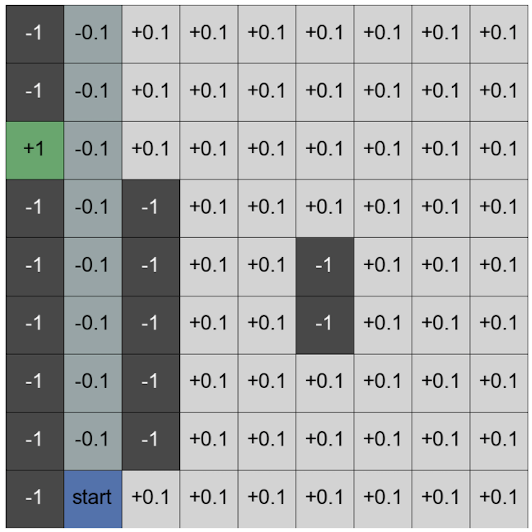
(a)

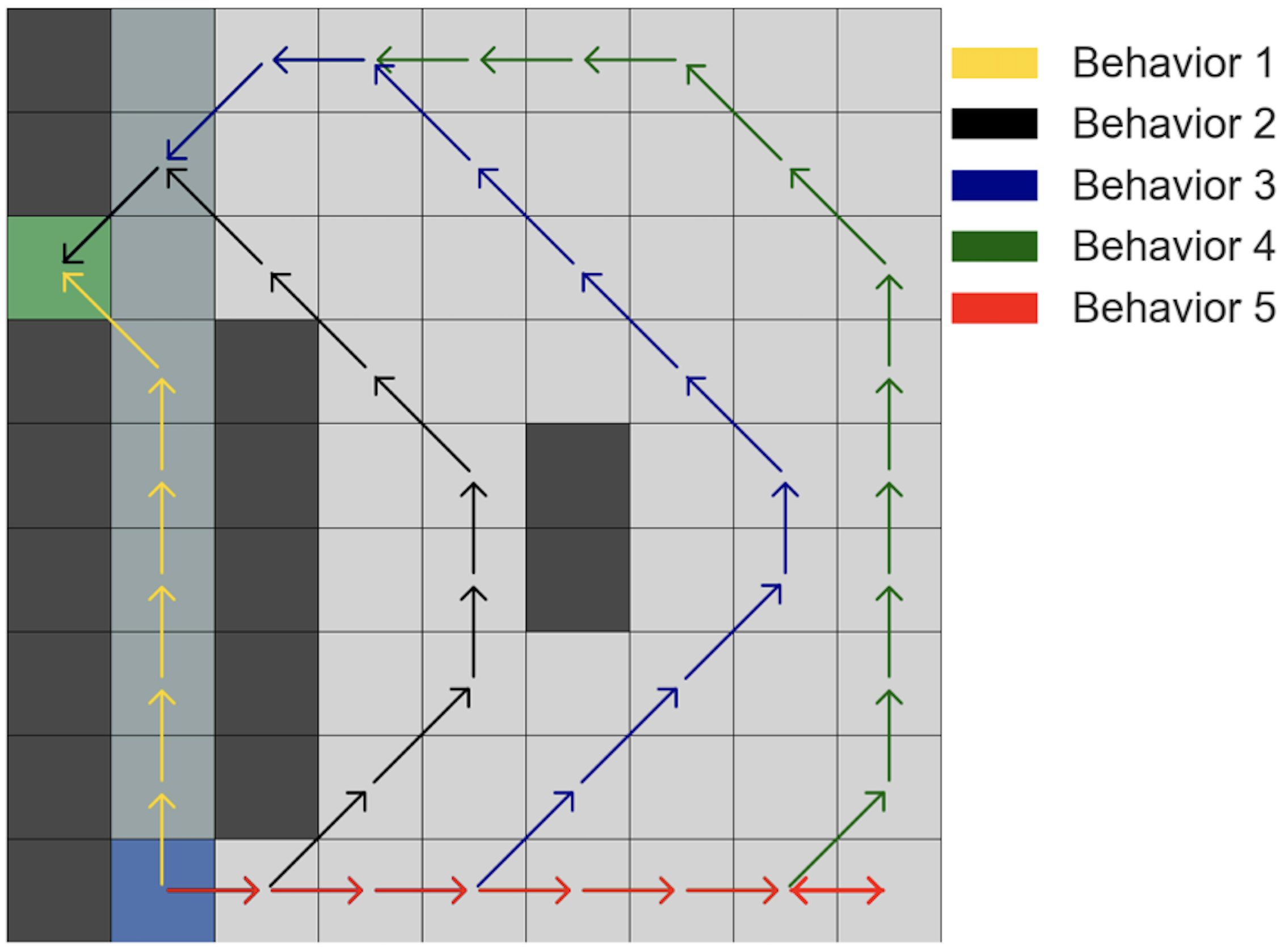
(b)

Figure 1: (a) Grid World layout showing the reward structure. (b) The five behavior profiles of risk-sensitive policies through the Grid World. These five paths correspond to the maximum likelihood paths of agents with various parameter combinations for their prospect, $\ell$-prospect and entropic map value functions. To generate each behavior with the prospect and $\ell$-prospect value functions, the following parameter combinations ($\{k_{-},k_{+},\zeta_{-},\zeta_{+}\}$) were used: Behavior 1: $\{0.1,1.0,0.5,1.5\}$; Behavior 2: $\{1.0,1.0,1.0,1.0\}$; Behavior 3: $\{1.0,1.0,1.1,0.9\}$; Behavior 4: $\{5.0,1.0,1.1,0.8\}$; Behavior 5: $\{5.0,1.0,1.5,0.7\}$. To generate the behaviors with the entropic map value function, we varied $\lambda$ from $1$ to $-1$.

IV-A1 Setup

Our instantiation of Grid World is shown in Fig. 1a. An agent operating in this MDP starts in the blue box and aims to maximize their value function over an infinite time horizon. Every square in the grid represents a state, and the action space is $A=\{N,NE,E,SE,$ $S,SW,W,NW\}$. Each action corresponds to a movement in the specified direction (where we have used the usual abbreviations for directions). The black and green states are absorbing, meaning that once an agent enters that state they can never leave no matter their action. In all the other states, the agent moves in their desired direction with probability $0.93$ and they move in any of the other seven directions with probability $0.01$. To make the grid finite, any action taking the agent out of the grid has probability zero, and the other actions are re-weighted accordingly. The reward structure of our instantiation of the Grid World is shown in Fig. 1a as well. The agent gets a reward of $-1$ and $+1$ for being in the black and green states respectively. In the darker gray states, the agent gets a reward of $-0.1$. In all other states the agent is given a reward of $+0.1$.

Value Function	Prospect		$\ell$-prospect		Entropic
Behavior	Mean	Variance	Mean	Variance	Mean	Variance
Behavior 1	$1.9$e-2	$6.3$e-$4$	$1.3$e-2	$2.3$e-$4$	$1.6$e-$3$	$5.1$e-$6$
Behavior 2	$1.5$e-2	$2.0$e-$4$	$1.0$e-2	$9.6$e-$5$	$2.6$e-$4$	$1.4$e-$7$
Behavior 3	$2.0$e-2	$3.6$e-$4$	$1.1$e-2	$1.3$e-$4$	$2.2$e-$3$	$1.5$e-$5$
Behavior 4	$1.6$e-2	$2.0$e-$4$	$1.2$e-2	$1.4$e-$4$	$4.6$e-$4$	$1.8$e-$7$
Behavior 5	$4.7$e-2	$3.0$e-$3$	$1.0$e-2	$3.4$e-$4$	$6.6$e-$4$	$2.2$e-$7$

(a)

Value Function	Mean	Variance
Prospect	$1.5$e-2	$1.6$e-$4$
$\ell$-prospect	$1.5$e-2	$1.6$e-$4$
Entropic Map	$5.4$e-2	$1.4$e-$2$

(b)

TABLE I: Mean and variance of the TV distance across all states in the grid of the between the true policy and the policy under the learned value function. We note that we present the best of five randomly sampled initial sets of parameters. (a) Results for learning with the same type of value function as that of the agent. (b) Results learning with different models than the true agent: 10,000 trajectories are sampled from the policy of an agent with the prospect value function with $\{k_{-},k_{+},\zeta_{-},\zeta_{+}\}=\{2.0,1.0,0.9,0.7\}$; prospect, $\ell$-prospect, and entropic map value functions are learned from this data.

IV-A2 Learning with the correct model of the value function

This experiment is intended to validate our approach on a simple example. We trained agents with various parameter combinations of the four value functions described in Section II. The resulting policies of these agents are classified into five behavior profiles via their maximum likelihood path through the MDP. These behaviors are outlined in Fig. 1b. Each behavior corresponds to the maximum likelihood path resulting from a different risk profile: Behavior 1 corresponds to a profile that is risk-seeking on gains, Behavior 2 corresponds to a profile that is risk neutral on gains and losses (this is also the behavior corresponding to the non-risk-sensitive reinforcement learning approach), and Behaviors 3-5 correspond to behaviors that are increasingly risk averse on losses and increasingly weigh losses more than gains.

We sampled 1,000 trajectories from the policies of these agents and used the data to learn the value function of the agent using our gradient-based approach. In this experiment, the learned value function is of the same type as that of the agent. For example, the data sampled from the policy of an agent having a prospect value function and exhibiting Behavior 1 is used to learn the parameters of a prospect value function. We note that due to the non-convexity of the problem, we use five randomly generated initial parameter choices.

The results we report are associated with the value function that achieves the minimum value of the objective. In Table Ia, we report the mean TV distance between the two policies across all states, as well as the variance in the TV distance across states. In all the cases considered in Table Ia, the learned value functions produce policies that correctly match the maximum likelihood path of the true agent.

We remark that the performance for learning a prospect value function was consistently worse than learning an $\ell$-prospect function. This is most likely due to the fact that the prospect value function is not Lipschitz around the reference point. Thus, we have no guarantees of differentiability of $Q^{\ast}$ with respect to $\theta$ for the prospect value function. This translates to numerical issues in calculating the gradient which, in turn, results in worse performance.

The entropic value function performs best of the four value functions, primarily due to the fact that there is only one parameter to learn, and the rewards and losses are all relatively small. In fact, in all the cases the learned entropic map value function coincided with the true value function of the agent, thereby indicating that the objective function was relatively convex around the parameter values we tried.

IV-A3 Learning with an incorrect model of the value function

The second experiment consists of learning different types of value functions from the same dataset. This is a more realistic experiment since the value function of human subjects will very likely be different than any model we could choose. The motivation for this experiment is to ensure that the results and risk-profiles learned were consistent across our choice of model.

The experiment uses 10,000 samples from an agent with a prospect value function and learned prospect, $\ell$-prospect, and entropic map value functions. The mean TV distance between the policy of the true agent and the policies under the learned value functions are shown in Table Ib. The true agent’s value function has parameters $\{k_{-},k_{+},\zeta_{-},\zeta_{+}\}=\{2.0,1.0,0.9,0.7\}$—that is, it is risk-seeking in losses, risk-averse in gains, and loss averse.

Again, the learned value functions all have policies that replicated the maximum likelihood behavior of the true agent. We note that the $\ell$-prospect and prospect functions perform as well as each other on this data, but the $\ell$-prospect function showed none of the numerical issues that we encountered with the prospect function (see Section IV-C for further detail on numerical considerations). Further, learning with the $\ell$-prospect function is markedly faster than with the prospect function. Again, this is most likely due to the fact that the prospect function is not locally Lipschitz continuous around the reference point. Thus, the values of $\alpha$ required to make the various contraction maps converge to their fixed points are vanishingly small. This results in slow convergence.

The fact that the entropic value function does not perform as well is most likely due to the fact that it cannot accurately match the shape of the prospect function at these values; e.g., the entropic map is always either convex or concave.

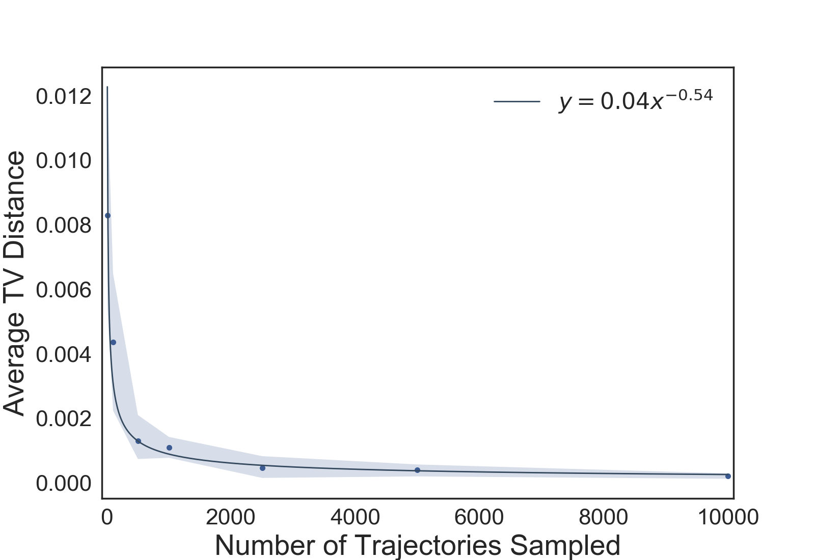
Figure 2: The mean TV distance across all states between the agent’s policy and the policy under the learned value function, as a function of the number of trajectories in the dataset. To construct each data point, we sample five different datasets of the same number of trajectories from the agent’s policy. We try five random initial parameter values per dataset and take the value function that achieves the minimum value of the objective. We calculate the mean TV distance between the policy of the agent and the policy under the learned value function for each dataset and then average these values. The bars show the 95% confidence interval around the mean of the five datasets of the given size. We note that the trendline $y=0.04x^{-0.54}$ is the best fit of the form $y=ax^{b}$ to the data points, for constant terms $a,b$.

IV-A4 Qualitative results on sample complexity

One of the challenges in modeling human decision-making is the lack of access to large datasets, particularly when it comes to sequential decisions that are made over longer periods of time. This is counter to the usual learning scenarios addressed in the much of the learning literature. For instance, if the focus is learning to control a robot, then it may be possible to generate a large number of demonstrations very quickly. This motivates our third experiment with the Grid World MDP—i.e. an experiment that allows us to better understand how the performance of our approach varies with the size of the dataset.

In this experiment, we first train an agent with an entropic map value function and then create sets of sample trajectories from the agent’s policy varying between zero and 10,000 in size. Next, using each of these sample sets, we learn the value function via our approach and plot the mean TV distance across all states between the true policy of the agent and the policy under the learned value function. This is shown in Fig. 2.

First, we note that more data does translate to consistently better results. This matches our intuition that the better our data matches the policy of the true agent, the better we can learn a value function that would be associated with that policy. Of particular interest, though, is the rate at which the average TV across all the states decreases with the number of trajectories sampled. The rate, which is on the order of $x^{-0.54}$, is very close to the asymptotic rate, derived in Section III-C, of $O(x^{-1/2})$. This suggests that the dominating factor in the performance of our algorithm is how well our data matches the underlying policy, and not the non-convexity of the objective function. In fact, this provides empirical evidence that the second term in (44)—i.e. $\delta(\hat{\pi}_{n}(\cdot|x),\pi_{\theta}(\cdot|x))$—must also be $O(x^{-1/2})$.

IV-B A Passenger’s View of Ride-Sharing

In addition to the Grid World example, we explore a ride-sharing example for which the MDP is created from real-world data and we simulate agents with different risk preference and loss aversion profiles.

Many ride-sharing companies set prices based on both supply of drivers and demand of passengers. From the passenger’s viewpoint, we model the ride-sharing MDP as follows. The action space is $A=\{0,1\}$ where $0$ corresponds to ‘wait’ and $1$ corresponds to ‘ride.’ The state space $X=\mathcal{X}\times\mathcal{T}\cup\{x_{\text{f}}\}$ where $\mathcal{X}$ is a finite set of surge price multipliers, $\mathcal{T}=\{0,\ldots,T_{\text{f}}\}$ is the part of the state corresponding to the time index, and $x_{\text{f}}$ is a terminal state representing the completed ride that occurs when a ride is taken. At time $t$, the state is notationally given by $(x_{t},t)$. The reward $r_{t}$ is modeled as a random variable that depends on the current price as well as a random variable $Z(t)$ for travel time. In particular, for any time $t<T_{\text{f}}$ the reward is given by

$$R(x_{t},a_{t})=\left\{\begin{array}[]{ll}\bar{r},&\ a_{t}=0\ (\text{'wait'})\\ \tilde{r}_{t},&\ a_{t}=1\ (\text{'ride'})\end{array}\right.$$ (45)

with $\bar{r}<0$ a constant and $\tilde{r}_{t}={S}_{t}-x_{t}(p_{\text{base}}+p_{\text{mile}}D+p_{\text{min}}Z(t))$ where $D$ is the distance in miles, ${S}_{t}$ is a time dependent satisfaction (we selected it to linearly decrease in time from some initial satisfaction level), and $p_{\text{base}}$, $p_{\text{mile}}$, and $p_{\text{min}}$ are the base, per mile, and per min prices, respectively.

At the final time $T_{\text{final}}$, the agent is forced to take the ride if they have not selected to take a ride at a prior time. This reflects the fact that the agent presumably needs to get from their origin to their destination and the reward structure reflects the dissatisfaction the agent feels as a result of having to ultimately take the ride despite the potential desire to wait.

Using the Uber Movement platform for travel time statistics, base pricing data and surge pricing data for Washington D.C., we examined several locations and hours which have different characteristics in terms of travel time and price statistics. We generate the distribution for $Z(t)$ from these data sets as well as the surge price intervals and transition probability matrix. Since the core risk-sensitive behaviors we observe are similar across the different locations, we report only on one.

Specifically, we report on a ride-sharing MDP generated with an origin and destination of GPS$=(-77.027046,$ $38.926749)$ and GPS$=(-76.935773,$ $38.885964)$, respectively, in Washington D.C. at 5AM.

Value Function	Prospect		Entropic		Prospect/$\ell$-prospect
Preferences	Mean	Variance	Mean	Variance	Mean	Variance
RA Gains/RS Losses (Entropic: RA)	1.3e-2	3.5e-4	0.9e-3	1.0e-6	1.0e-2	1.4e-4
Risk-Neutral	0.6e-2	4.9e-5	1.4e-3	2.0e-6	6.6e-3	1.0e-4
RS Gains/RA Losses (Entropic: RS)	1.1e-2	1.7e-4	1.1e-3	1.5e-6	1.1e-2	1.1e-4

TABLE II: Averaged TV error and variance over 10 different initializations of the algorithm for different risk-preference profiles. The last column shows the error when using an $\ell$-prospect agent with $\upepsilon=1$e-2 to learn a prospect agent. We use the following abbreviations: Risk-Averse (RA); Risk-Seeking (RS).

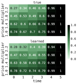
(a)

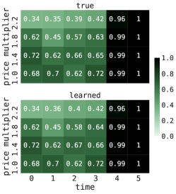
(b)

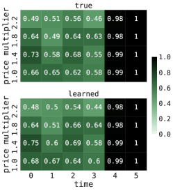
(c)

Figure 3: Plots showing the probabilities of taking a ride in each state under the true and learned optimal policies for true and learned agents with prospect value functions. The true agent has prospect gain parameters of $k_{+}=0.5$ and $k_{-}=1.0$ for all three plots. The value function used for the right most graphic (Fig. 4c) is most representative of human decision-making since humans tend to be risk-averse in gains, risk-seeking in losses, are loss averse. In these plots, the trend we see is that the more risk-averse, the less likely they policy suggests taking the ride.

The transition probability kernel $P:X\times A\times X\rightarrow[0,1]$ is estimated from the ride-sharing data. The travel-time data is available on an hourly basis and the price change data is available on a three minute basis. Hence, we use the three minute price change data for each hour to derive a static transition matrix by empirically estimating the transition probabilities where we bin prices in the following way. For prices in $[1.0,1.2)$, $x=1.0$; for prices in $[1.2,1.6)$, $x=1.4$; for prices in $[1.6,2.0)$, $x=1.8$; otherwise $x=2.2$. Hence, $\mathcal{X}=\{1.0,1.4,1.8,2.2\}$. In the time periods we examine, the max price multiplier was $2.2$. We set the reference point $y_{0}$ and acceptance level $v_{0}$ to be zero.

With this model, the transition matrix for the price multipliers is given by

$$P=\begin{bmatrix}0.876&0.099&0.017&0.008\\ 0.347&0.412&0.167&0.074\\ 0.106&0.353&0.259&0.282\\ 0.086&0.219&0.143&0.552\end{bmatrix}$$ (46)

for each time. The travel time distribution is a standard normal distribution truncated to the upper and lower bounds specified by the Uber Movement data. Measured in seconds, we use location parameter $2371$, scale parameter $100$, and $1554$ and $3619$ as the upper and lower bound, respectively.

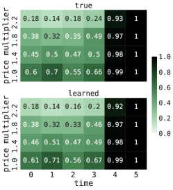
(a)

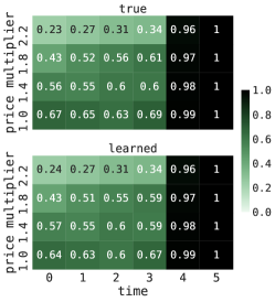
(b)

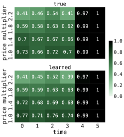
(c)

Figure 4: Plots showing the probabilities of taking a ride in each state under the true and learned optimal policies for true and learned agents with prospect value functions. The true agent has prospect parameters of $\zeta_{-}=\zeta_{+}=1.0$ for all three plots, while we vary $(k_{+},k_{-})$ to capture different degrees of loss-aversion. In these plots, the trend we see is that the more loss-averse the agent (under both the learned and true value functions), the more likely they are to take the ride.

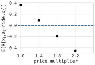
Figure 5: Expected rewards for each time step in the ride-sharing example. Notice that the rewards can either be gains (positive values) or losses (negative values) given that we take the reference point to be $y_{o}=0$.

The graphics in Fig. 3 and Fig. 4 show the state space as a grid with the probability of taking a ride under the true and learned optimal policies overlaid on each state. For the examples depicted in these figures, we consider the true and learned agents to have prospect value functions.

In Fig. 3, we fix the true agent’s parameters to show a range of behaviors from risk-seeking in losses/risk-averse in gains to risk-averse in losses/risk-seeking in gains. There is empirical evidence supporting the fact that humans are more like the former. Moreover, in these examples we use $(k_{+},k_{-})=(0.5,1)$ to capture that humans tend to be loss-averse—that is, for losses and gains of equal value, the loss is perceived as more significant.

On the other hand, in Fig. 4 we fix the true agent’s parameters to show a range of behaviors depending on the degree of loss-aversion. In particular, we fix $\zeta_{-}=\zeta_{+}=1$ and vary the ratio of $k_{-}$ to $k_{+}$, where a higher ratio corresponds to more loss averse preferences.

In each of the graphics in Fig. 3 and Fig. 4, we see that the learned policy is very close to the true policy. In addition, in Fig. 3, we observe that the more risk-averse the agent is (in gains or losses), the more likely they are to take the ride. This trend can be seen by noting the sign of the expected rewards—in Fig. 5, we see that the reward is positive for $x_{t}\in\{1.0,1.4\}$ and is negative for $x_{t}\in\{1.8,2.2\}$—and examining the corresponding rows in Fig. 3 for negative and positive rewards. In Fig. 4, observe that the more loss averse the agent, the more likely they are to take the ride uniformly. This is reasonable as the satisfaction level is linear decreasing in time.

In Table II, we show the mean and variance of the total variation error for the ride-sharing example where we varied the risk preference profiles, holding $(k_{-},k_{+})=(1,1)$, using agents with prospect and entropic value functions. In addition, we show the error for different risk profiles when we learn a true prospect agent with an $\ell$-prospect agent. Recall that the prospect value function does not meet the requirements of our theorem whereas the $\ell$-prospect value function does as it is Lipschitz.

IV-C Numerical Considerations

We end the experimental results section with some observations on the convergence speed and the implementation of Algorithm 1.

First, we note that the two contraction mappings (33) and (32) are sensitive to the learning rate $\alpha$. A very small choice of $\alpha$ results in convergence of the sequence of Q-functions to the fixed point being too slow to be practically useful. On the other hand, a large choice of $\alpha$ makes the sequence diverge. Thus, choosing $\alpha$ has a large effect on the runtime of the overall algorithm as the computation of $Q^{\ast}$ and $D_{\theta}Q^{\ast}$ both depend on the choice of $\alpha$.

We further remark that numerical observations suggest that the condition $\alpha\in(0,\min\{L^{-1},1\}]$ is fairly restrictive and that larger values of $\alpha$ give faster convergence. Hence, our implementation of Algorithm 1 includes an adaptive scheme to find the largest possible $\alpha$. In particular, if two consecutive iteration elements in the sequence are observed to diverge in the $L_{\infty}$ norm, we decrease $\alpha$ by a fixed constant. As long successive elements in the sequence converge, we periodically increase $\alpha$ by another constant. This allows us to noticeably speed up the implementation of our algorithm. Adaptively choosing the step-size $\alpha$ also allows us to train the prospect function agents more accurately, since these were particularly susceptible to changes in the value of $\alpha$ due to the fact that the value function is non-Lipschitz around the reference point.

To speed up the gradient-descent algorithm, we also implement a back-tracking line search. We do this to address the computationally intensive gradient calculation. Specifically, the line-search allows us to exploit each gradient calculation fully. The backtracking line search also leads to a noticeable speed up in the implementation of our algorithm, which allows us to tackle larger MDPs.

V Related Work

Before concluding, we draw some comparisons between our work and that of others on related topics.

The primary motivation for most other works in this domain is to learn a prescriptive model for humans amidst autonomy. For example, in [7], their approach to learning the decision-making model is to parameterize unknown quantities of interest, sample the parameter space, and use a model selection criteria (i.e. Bayesian information criteria) to select parameters that best fit the observed behavior. In contrast, we derive a well-formulated gradient-based procedure for finding the value function and policy best matching the observed behavior. Moreover, we introduce new value functions that satisfy our theorems for the forward and inverse problems while retain the salient features of the empirically observed behavioral models.

Another related work is [10]. The authors take a similar approach to ours in leveraging risk metrics to capture risk sensitivity. However, they focus their efforts on estimating the risk metric by leveraging the well-known representation theorem for coherent risk metrics [23]. They couple the resulting optimization problem with classical inverse reinforcement learning procedures for learning the reward (that is, they parameterize the reward function over a set of basis functions), yet their approach does not differentiate between the reward and the decision-making model. In contrast, we consider a broad class of risk metrics generated by value functions via acceptance sets, formulate the MDP model based on the risk metric, and learn the parameters of the value function that generates the risk metric and results in a policy that best matches the agent’s observed behavior. The parameters of the value function, which ultimately drive the decision-making model, are highly interpretable in terms of the degree of risk sensitivity and loss aversion. Thus, our technique supports prescriptive and descriptive analysis, both of which are important for the design of incentives and policies that takes into consideration the nuances of human decision-making behavior.

Finally, as noted in the introduction, the results in this paper significantly extend our previous work [15]. We (i) provide new convergence guarantees for the forward risk-sensitive reinforcement learning problem where behavioral-based value functions satisfy the assumptions and (ii) provide more extensive theoretical results on the gradient-based inverse risk-sensitive reinforcement learning problem including proofs for theorems appearing in the prior work.

VI Discussion

We present a new gradient based technique for learning risk-sensitive decision-making models of agents operating in uncertain environments. Specifically, we introduce a new forward risk-sensitive reinforcement learning procedure with convergence guarantees for which value functions retaining the fundamental shape of behavioral value functions satisfy the assumptions. Based on this learning algorithm, we introduce a well-formulated gradient-based inverse reinforcement learning algorithm to recover the parameters indicating the observed agent’s risk preferences. We demonstrate the algorithm’s performance for agents based on several types of behavioral models and do so on two examples: the canonical Grid World problem and a passenger’s view ride-sharing where the parameters of the ride-sharing MDP are learned from real-world data.

Looking forward, we are examining ways of designing mechanisms to adaptively produce the most informative demonstrations and to incentivize certain behaviors. This is challenging since some of the options in the state-action space may result in a very high risk to the agent and thus, the volatility introduced by inducing such state-action pairs may be viewed unfavorably by the agent causing them to completely opt-out.

-A Proof of Theorem 2

The proof of Theorem 2 relies on the following fixed point theorem.

Theorem 6 (Fixed Point Theorem [34, Theorem 2.2])

Let $(X,d)$ be a complete metric space and let $B_{r}(y)=\{x\in X|\ d(x,y)<r\}$ be a ball of radius $r$, where $r>0$, centered at $y\in X$. Let $f:B_{r}(y)\rightarrow X$ be a contraction map with contraction constant $h<1$. Further, assume that $d(y,f(y))<r(1-h)$. Then, $f$ has a unqiue fixed point in $B_{r}(y)$.

Proof:

We claim that $T$ is a contraction with constant $\bar{\alpha}=(1-\alpha(1-\gamma)\varepsilon_{K})$ where $\varepsilon_{K}=\min\{D\tilde{v}(y)|\ y\in I_{K}\}$. Indeed, let $y(Q(x,a))=r(x,a,w)+\gamma\max_{a^{\prime}}Q(x^{\prime},a^{\prime})-Q(x,a)$ be the temporal difference and define $g(x^{\prime},a^{\prime})=\max_{a^{\prime}}Q(x^{\prime},a^{\prime})$. For any $Q\in B_{K}(0)$ we note that the temporal differences are bounded—in fact, $y(Q(x,a))\in I_{K}=[-M-K,M+K]$. Due to the monotonicity assumption on $v$, we have that for any $y^{\prime},y\in I_{K}$, $\tilde{v}(y)-\tilde{v}(y^{\prime})=\xi(y-y^{\prime})$ for some $\xi\in[\varepsilon_{K},L]$. Recall the contraction map defined in (23):

$$(TQ)(x,a)= \alpha\mathbb{E}_{x^{\prime},w}\big{[}\tilde{v}\big{(}y(Q(x,a))\big{)}\big{]}+Q(x,a)$$ (47)

Then, for any $Q_{1}$ and $Q_{2}$, we have that

$$(TQ_{1}-TQ_{2})(x,a) =\alpha\mathbb{E}_{x^{\prime},w}[\tilde{v}(y(Q_{1}(x,a)))-\tilde{v}(y(Q_{2}(x,a)))]+Q_{1}(x,a)-Q_{2}(x,a)$$

$$\leq\alpha\mathbb{E}_{x^{\prime},w}[\xi_{x^{\prime},w}(\gamma(g_{1}(x^{\prime},a^{\prime})+g_{2}(x^{\prime},a^{\prime}))-Q_{1}(x,a)+Q_{2}(x,a))]$$

$$\quad+Q_{1}(x,a)-Q_{2}(x,a)$$

$$\leq\alpha\gamma\mathbb{E}_{x^{\prime},w}[\xi_{x^{\prime},w}(g_{1}(x^{\prime},a^{\prime})+g_{2}(x^{\prime},a^{\prime}))]$$

$$\ +(1-\alpha\mathbb{E}_{x^{\prime},w}[\xi_{x^{\prime},w}])(Q_{1}(x,a)-Q_{2}(x,a)).$$

Hence,

$$|(TQ_{1}-TQ_{2})(x,a)| \leq(1-\alpha(1-\gamma)\mathbb{E}_{x^{\prime},w}[\xi_{x^{\prime},w}])\|Q_{1}-Q_{2}\|_{\infty}$$

$$\leq(1-\alpha(1-\gamma)\varepsilon_{K})\|Q_{1}-Q_{2}\|_{\infty}.$$

We claim that the constant $\bar{\alpha}_{K}=1-\alpha(1-\gamma)\varepsilon_{K}<1$. Indeed, recall that $0<\alpha\leq\min\{1,L^{-1}\}$ so that if $\alpha=L^{-1}$, then $\bar{\alpha}_{K}<1$ since $L=\max_{y\in I_{K}}D\tilde{v}(y)$ and $\varepsilon_{K}=\min_{y\in I_{K}}D\tilde{v}(y)$. On the other hand, if $\alpha=1$, then $1\leq L^{-1}\leq(\varepsilon_{K})^{-1}$ so that $\varepsilon_{K}\leq 1$ which, in turn, implies that $\bar{\alpha}_{K}<1$. If $0<\alpha<\min\{1,L^{-1}\}$, then $\bar{\alpha}_{K}<1$ follows trivially from the implications in the above two cases. Thus, $T$ is a contraction on $B_{K}(0)$ with the constant $\bar{\alpha}_{K}=(1-\alpha(1-\gamma)\varepsilon_{K})<1$. ∎

Proof:

Suppose $K$ is chosen such that

$$\frac{\max\{|\tilde{v}(M)|,|\tilde{v}(-M)|\}}{1-\gamma}<K\min_{y\in I_{K}}D\tilde{v}(y).$$ (48)

Now, we argue that $T$ applied to the zero map, $0\in B_{K}(0)$, is strictly less than $K(1-\bar{\alpha}_{K})$. Indeed, for any $\alpha\in(0,\min\{1,L^{-1}\}]$,

$$\|T(0)\| \leq\alpha\max\{|v(M)|,|v(-M)|\}$$

$$<(1-\gamma)K\varepsilon_{K}\alpha=K(1-\bar{\alpha}_{K})$$

Combinging the above fact with the fact that $T$ is a contraction, the assumptions of Theorem 6 hold and, hence there is a unique fixed point $Q^{\ast}(x,a)\in B_{K}(0)$ for each $(x,a)\in X\times A$. ∎

-B Proof of Proposition 3

Recall that $\tilde{v}\equiv v-v_{0}$. For different value functions, Proposition 3 claims that the condition of Theorem 2.b,

$$\frac{\max\{|\tilde{v}(M)|,|\tilde{v}(-M)|\}}{(1-\gamma)}<K\min_{y\in I_{K}}D\tilde{v}(y),$$ (49)

holds.

Proof:

Suppose $v$ satisfies Assumption 1 and that for some ${\varepsilon}>0$, ${\varepsilon}<\frac{v(y)-v(y^{\prime})}{y-y^{\prime}}$ for all $y\neq y^{\prime}$. Then there exists a value of $K$, say $\bar{K}$, such that (49) holds for all $K>\bar{K}$. Indeed since $\min_{K>0}\varepsilon_{K}>{\varepsilon}$, for all $K$ satisfying

$$\frac{\max\{|\tilde{v}(M)|,|\tilde{v}(-M)|\}}{{\varepsilon}(1-\gamma)}<K,$$

(49) must hold. ∎

Proof:

We now show that for the $\ell$-prospect value function, (49) holds for any choice of parameters $(k_{-},k_{+},\zeta_{-},\zeta_{+})$. Indeed, for $\zeta_{+},\zeta_{-}\geq 1$ and any choice of $k_{-},k_{+}$,

$$\min_{K>0}\varepsilon_{K}>{\varepsilon}>0$$

where ${\varepsilon}=\min\{\lim_{y\uparrow 0}D\tilde{v}(y),\lim_{y\downarrow 0}D\tilde{v}(y)\}$. Therefore, with $\zeta_{+},\zeta_{-}\geq 1$, for any $K$ such that

$$\frac{\max\{|\tilde{v}(M)|,|\tilde{v}(-M)|\}}{{\varepsilon}(1-\gamma)}<K,$$

(49) must hold. For the case when either $\zeta_{+}<1$ or $\zeta_{-}<1$ or both, we note that

$$\min_{y\in I_{K}}D\tilde{v}(y)=\min\left\{\min_{y\in\{M+K,-M-K\}}D\tilde{v}(y),{\varepsilon}\right\}.$$

so that we need only show that for $\zeta_{+}<1$ and $\zeta_{-}<1$, there exists a $K$ such that

$$\frac{\max\{|\tilde{v}(M)|,|\tilde{v}(-M)|\}}{1-\gamma}<KD\tilde{v}(K+M)$$ (50)

and

$$\frac{\max\{|\tilde{v}(M)|,|\tilde{v}(-M)|\}}{1-\gamma}<KD\tilde{v}(-K-M),$$ (51)

respectively. Note that

$$D\tilde{v}(y)=\left\{\begin{array}[]{ll}k_{+}\zeta_{+}(y-y_{0}+\upepsilon)^{\zeta_{+}-1},&\ y\geq y_{0}\\ k_{-}\zeta_{-}(y_{0}-y+\upepsilon)^{\zeta_{-}-1},&\ y<y_{0}\end{array}\right.$$

Without loss of generality, we show (50) must hold for $\zeta_{+}<1$ and reference point $y_{0}=0$ (the proof for $\zeta_{-}<1$ follows an exactly analogous argument). Plugging $D\tilde{v}(K+M)$ in and rearranging, we get that we need to find a $K$ such that

$$\frac{\max\{|\tilde{v}(M)|,|\tilde{v}(-M)|\}}{(1-\gamma)\xi_{+}k_{+}}<K(K+M+\upepsilon)^{\xi_{+}-1}$$

Since the right-hand side above is a function of $K$ that is zero at $K=0$ and approaches infinity as $K\rightarrow\infty$, and the left-hand side is a finite constant, there is some $\bar{K}$ such that for all $K>\bar{K}$, the above holds. Thus, for the $\ell$-prospect value function, our assumptions are satisfied and there always exists a value of $K$ to choose in Theorem 2.b. ∎

Proof:

Suppose $v$ is an entropic map. We note that, for the entropic map, $\min_{y\in I_{K}}D\tilde{v}(y)$ must occur at either $K+M$ or $-K-M$ if $\lambda<0$ or $\lambda>0$, respectively. Without loss of generality, let $\lambda>0$. First, consider that the derivative of $\tilde{v}$,

$$D\tilde{v}(y)=(\lambda)^{-1}e^{\lambda y},$$

is minimized on $I_{K}$ at $-M-K$ for any $M$ and $K$. Moreover, $|\tilde{v}(M)|>|\tilde{v}(-M)|$. Hence, with $K=\lambda^{-1}$, we can derive conditions on $\lambda$ for which (49) holds. In other words, with the specified $K$, we use (49) to dertermine which values of $\lambda$ are admissible. Indeed, from (49), we have

$$(1-\gamma)^{-1}e^{\lambda M}<(\lambda)^{-1}e^{-\lambda M-1}$$

which reduces to $\lambda e^{2\lambda M}<(1-\gamma)e^{-1}.$ Let $x=2\lambda M$, so that

$$xe^{x}<2M(1-\gamma)e^{-1}.$$

Now, we can apply the Lambert $W$ function which satisfies $W(xe^{x})=x$ for $x\geq 0$, to get that

$$x<W(2M(1-\gamma)e^{-1}),$$

so that

$$\lambda<(2M)^{-1}{W(2M(1-\gamma)e^{-1})}.$$

Thus, if $|\lambda|<(2M)^{-1}{W(2M(1-\gamma)e^{-1})}$, then for the choice $K=\frac{1}{\lambda}$, (49) holds so that Theorem 2.b holds for the entropic map. ∎

-C Proof of Theorem 4

We remark that the gradient algorithm and Theorem 4 are consistent with the gradient descent framework which uses the contravariant gradient for learning as introduced in [35] for Riemannian parameter spaces $\Theta$. Of course, when $\Theta$ is Euclidean and the coordinate system is orthonormal, the gradient we normally use (covariant derivative) coincides with the contravariant gradient. However, using the covariant derivative does not generalize to admissible parameter spaces with more structure.

Moreover, as is pointed out in [30], the trajectories that result from the solution to the gradient algorithm are equivalent up to reparameterization through a smooth invertible mapping with a smooth inverse. Contravariant gradient methods have been shown to be asymptotically efficient in a probabilistic sense and thus, they tend to avoid plateaus [35, 36].

Before we dive into the proof of Theorem 4, let us introduce some definitions and useful propositions.

Definition 4 (Fréchet Subdifferentials)

Let $U$ be a Banach space and $U^{\ast}$ its dual. The Fréchet subdifferential of $f:U\rightarrow\mathbb{R}$ at $u\in U$, denoted by $\partial f(u)$ is the set of $u^{\ast}\in U^{\ast}$ such that

$$\lim_{h\rightarrow 0}\inf_{h\neq 0}\|h\|^{-1}\left(f(u+h)-f(u)-\langle u^{\ast},u\rangle\right)\geq 0.$$ (52)

Proposition 4 ([30, 37])

For a finite family $(f_{i})_{i\in I}$ of real-valued functions (where $I$ is a finite index set) defined on $U$, let $f(u)=\max_{i\in I}f_{i}(u)$. If $u^{\ast}\in\partial f_{i}(u)$ and $f_{i}(u)=f(u)$, then $u^{\ast}\in\partial f_{i}(u)$. If $f_{1},f_{2}:U\rightarrow\mathbb{R}$, $\alpha_{1},\alpha_{2}\geq 0$, then $\alpha_{1}\partial f_{1}+\alpha_{2}\partial f_{2}\subset\partial(\alpha_{1}f_{1}+\alpha_{1}f_{2})$.

Proposition 5 ([30, 38])

Suppose that $(f_{n})_{n\in\mathbb{N}}$ is a sequence of real-valued functions on $U$ which converge pointwise to $f$. Let $u\in U$, $u_{n}^{\ast}\in\partial f_{n}(u)\subset U^{\ast}$ and suppose that $(u_{n}^{\ast})$ is weak^∗–convergent to $u^{\ast}$ and is bounded. Moreover, suppose that at $u$, for any $\varepsilon>0$, there exists an $N>0$ and $\delta>0$ such that for any $n\geq N$, $h\in B_{U}(0,\delta)$, a $\delta$–ball around $0$, $f_{n}(u+h)\geq f_{n}(u)+\langle u_{n}^{\ast},h\rangle-\varepsilon\|h\|$. Then $u^{\ast}\in\partial f(u)$.

We now provide the proof for parts (a) and (b) of Theorem 4.

Proof:

Let $Q_{0}(x,a,\theta)\equiv 0$. Then it is trivial that $Q_{0}(x,a,\theta)$ is locally Lipschitz in $\theta$ on $\Theta$. Supposing that $Q_{t}(x,a,\theta)$ is $L_{t}$–locally Lipschitz in $\theta$, then we need to show that $TQ_{t}(x,a,\theta)$ is locally Lipschitz which we recall is defined by

$$(TQ)(x,a,\theta)=\alpha\mathbb{E}_{x^{\prime},w}\tilde{v}(y(\theta),\theta)+Q(x,a,\theta)$$ (53)

where $y(\theta)=r(x,a,w)+\gamma\max_{a^{\prime}\in A}Q(x^{\prime},a^{\prime},\theta)-Q(x,a,\theta)$.

Since $\tilde{v}\equiv v-v_{0}$, it also satisfies Assumption 2. Let $L_{y}=\max\{L_{y}(\theta)|\theta\in\Theta\}$ and define $g_{t}(x,\theta)=\max_{a^{\prime}}Q_{t}(x,a^{\prime},\theta)$. Note that since $Q_{t}$ is assumed Lipschitz with constant $L_{t}$, so is $g_{t}$. Surpressing the dependent of $TQ$ on $(x,a)$, we have that

$$TQ_{t}(\theta)-TQ_{t}(\theta^{\prime}) =\alpha\mathbb{E}_{x^{\prime},w}[\tilde{v}(y(\theta),\theta)-\tilde{v}(y(\theta^{\prime}),\theta^{\prime})]+Q_{t}(x,a,\theta)-Q_{t}(x,a,\theta^{\prime})$$

$$=\alpha\mathbb{E}_{x^{\prime},w}[\tilde{v}(y(\theta),\theta)-\tilde{v}(y(\theta^{\prime}),\theta)+\tilde{v}(y(\theta^{\prime}),\theta)-\tilde{v}(y(\theta^{\prime}),\theta^{\prime})]$$

$$\qquad+Q_{t}(\theta)-Q_{t}(\theta^{\prime}).$$

Due to the monotonicity of $\tilde{v}$ in $y$, we know that for all $y_{1},y_{2}$ there exists $\xi\in[\varepsilon,L_{y}]$ such that

$$\tilde{v}(y_{1},\theta)-\tilde{v}(y_{2},\theta)=\xi(y_{1}-y_{2}).$$

Hence,

$$\mathbb{E}_{x^{\prime},w}[\tilde{v}(y(\theta),\theta)-\tilde{v}(y(\theta^{\prime}),\theta)+\tilde{v}(y(\theta^{\prime}),\theta)-\tilde{v}(y(\theta^{\prime}),\theta^{\prime})]$$

$$\ \ =\mathbb{E}_{x^{\prime},w}[\xi_{x^{\prime},w}(y(\theta)-y(\theta^{\prime}))+\tilde{v}(y(\theta^{\prime}),\theta)-\tilde{v}(y(\theta^{\prime}),\theta^{\prime})]$$

where we simply denote the dependence of $\xi$ on $x^{\prime}$ and $w$, the components subject to randomness. Then,

$$TQ_{t}(\theta)-TQ_{t}(\theta^{\prime}) =\alpha\mathbb{E}_{x^{\prime},w}\big{[}\xi_{x^{\prime},w}(y(\theta)-y(\theta^{\prime}))+\tilde{v}(y(\theta^{\prime}),\theta)-\tilde{v}(y(\theta^{\prime}),\theta^{\prime})\big{]}$$

$$\ \ \ \ +Q_{t}(\theta)-Q_{t}(\theta^{\prime})$$

$$=\alpha\gamma\mathbb{E}_{x^{\prime},w}[\xi_{x^{\prime},w}(g_{t}(x^{\prime},\theta)-g_{t}(x^{\prime},\theta^{\prime}))]-\alpha\mathbb{E}_{x^{\prime},w}[\xi_{x^{\prime},w}(Q_{t}(\theta)-Q_{t}(\theta^{\prime}))]$$

$$\ \ \ \ +\alpha\mathbb{E}_{x^{\prime},w}[\tilde{v}(y(\theta^{\prime}),\theta)-\tilde{v}(y(\theta^{\prime}),\theta^{\prime})]+Q_{t}(\theta)-Q_{t}(\theta^{\prime})$$

$$\quad=\alpha\gamma\mathbb{E}_{x^{\prime},w}[\xi_{x^{\prime},w}(g_{t}(x^{\prime},\theta)-g_{t}(x^{\prime},\theta^{\prime}))]-\alpha\mathbb{E}_{x^{\prime},w}[\xi_{x^{\prime},w}](Q_{t}(\theta)-Q_{t}(\theta^{\prime}))$$

$$\ \ \ \ +\alpha\mathbb{E}_{x^{\prime},w}[\tilde{v}(y(\theta^{\prime}),\theta)-\tilde{v}(y(\theta^{\prime}),\theta^{\prime})]+Q_{t}(\theta)-Q_{t}(\theta^{\prime})$$

$$\quad=(1-\alpha\mathbb{E}_{x^{\prime},w}[\xi_{x^{\prime},w}])(Q_{t}(\theta)-Q_{t}(\theta^{\prime}))+\alpha\gamma\mathbb{E}_{x^{\prime},w}[\xi_{x^{\prime},w}(g_{t}(x^{\prime},\theta)-g_{t}(x^{\prime},\theta^{\prime}))]$$

$$\ \ \ \ +\alpha\mathbb{E}_{x^{\prime},w}[\tilde{v}(y(\theta^{\prime}),\theta)-\tilde{v}(y(\theta^{\prime}),\theta^{\prime})]$$

so that

$$\|TQ_{t}(\theta)-TQ_{t}(\theta^{\prime})\|\leq ((1-\alpha(1-\gamma)\varepsilon)+\alpha L_{\theta})L_{t}\|\theta-\theta^{\prime}\|.$$

Hence, letting $\bar{\alpha}=1-\alpha(1-\gamma)\varepsilon$, we have that $TQ_{t}(\cdot,\cdot,\theta)$ is $L_{t+1}$–locally Lipschitz with $L_{t+1}=\bar{\alpha}L_{t}+\alpha L_{\theta}$. With $L_{0}=0$, by iterating, we get that

$$L_{t+1} =(\bar{\alpha}^{t}+\cdots+\bar{\alpha}+1)\alpha L_{\theta}.$$

As stated in Section III-B, $T$ is a contraction so that $T^{n}Q_{0}\rightarrow Q^{\ast}_{\theta}=Q^{\ast}(\cdot,\cdot,\theta)$ as $n\rightarrow\infty$. Hence, by the above argument, $Q^{\ast}_{\theta}$ is $\alpha L_{\theta}/(1-\bar{\alpha})$–Lipschitz continuous. ∎

Proof:

Consider a fixed vector $\theta\in\mathbb{R}^{d}$. We now show that the operator $S$ acting on the space of functions $\phi_{\theta}:X\times A\rightarrow\mathbb{R}^{d}$ and defined by

$$(S\phi_{\theta})(x,a) =\alpha\mathbb{E}_{x^{\prime},w}\big{[}D_{2}\tilde{v}(y(\theta),\theta)+D_{1}\tilde{v}(y(\theta),\theta)(\gamma\phi_{\theta}(x^{\prime},a_{x^{\prime}}^{\ast})-\phi_{\theta}(x,a))\big{]}+\phi_{\theta}(x,a)$$ (54)

is a contraction where $a_{x^{\prime}}^{\ast}$ is the action that maximizes $\sum_{a^{\prime}\in A}\pi(a|x)Q(x,a,\theta)$ for any greedy policy $\pi$ with respect to $Q_{\theta}$. Indeed,

$$(S\phi_{\theta}-S\phi_{\theta}^{\prime})(x,a) =\alpha\mathbb{E}_{x^{\prime},w}[D_{1}\tilde{v}(y(\theta),\theta)\big{(}\gamma(\phi_{\theta}(x^{\prime},a^{\ast}_{x^{\prime}})-\phi_{\theta}^{\prime}(x^{\prime},a^{\ast}_{x^{\prime}}))$$

$$\qquad-(\phi_{\theta}(x,a)-\phi_{\theta}^{\prime}(x,a))\big{)}]+\phi_{\theta}(x,a)-\phi_{\theta}^{\prime}(x,a)$$

$$\leq(1-\alpha(1-\gamma)\mathbb{E}_{x^{\prime},w}[D_{1}\tilde{v}(y(\theta),\theta)])\|\phi_{\theta}-\phi^{\prime}_{\theta}\|_{\infty}$$

so that, by Assumption 2,

$$\|(S\phi_{\theta}-S\phi_{\theta}^{\prime})(x,a)\|\leq(1-\alpha(1-\gamma)\varepsilon)\|\phi_{\theta}-\phi_{\theta}^{\prime}\|_{\infty}.$$

Thus, $\bar{\alpha}$ is the required constant for ensuring $S$ is a contraction. We remark that $S$ operates on each of the $d$ components of $\theta$ separately and hence, it is a contraction when restricted to each individual component.

Let $\pi$ denote a greedy policy with respect to $Q^{\ast}_{\theta}$ and let $\pi_{n}$ be a sequence of policies that are greedy with respect to $Q_{n}=T^{n}Q_{0}$ where ties are broken so that $\sum_{(x,a)\in X\times A}|\pi(a|x)-\pi_{n}(a|x)|$ is minimized. Then for large enough $n$, $\pi_{n}=\pi$. Denote by $S_{\pi_{n}}$ the map $S$ defined in (54) where $\pi_{n}$ is the implemented policy. Consider the sequence $\phi_{\theta,n}$ such that $\phi_{\theta,0}=0$ and $\phi_{\theta,n+1}=S_{\pi_{n}}\phi_{\theta,n}$. For large enough $n$, $\phi_{\theta,n+1}=S_{\pi}\phi_{\theta,n}$. Applying the (local) contraction mapping theorem (see, e.g., [39, Theorem 3.18]) we get that $\lim_{n\rightarrow\infty}S^{n}\phi_{0}$ converges to a unique fixed point.

Moreover, by induction and Proposition 4, $\phi_{\theta,n}(x,a)\in\partial_{\theta}Q_{n}(x,a,\theta)$. Hence, by Proposition 5, the limit is a subdifferential of $Q_{\theta}^{\ast}$ since $\tilde{v}$ is Lipschitz on $Y$ and $\Theta$ and the derivatives of $\tilde{v}$ are uniformly bounded. Since by part (a), $Q^{\ast}_{\theta}$ is locally Lipschitz in $\theta$, Rademacher’s Theorem (see, e.g., [31, Thm. 3.1]) tells us it is differentiable almost everywhere (expcept a set of Lebesgue measure zero). Since $Q_{\theta}^{\ast}$ is differentiable, its subdifferential is its derivative. ∎

-D Proof of Theorem 5

Given that the proof of Theorem 5 follows the same techniques as in Theorem 2 and Theorem 4, we provide largely an outline, directing the reader to the particular analogous components of the two proceeding theorems that are mimicked in creating the proof.

Proof:

For each $\theta$, the proof that $TQ(x,a,\theta)$ is a contraction, and thus has a fixed point $Q^{\ast}_{\theta}\in B_{K}(0)$, follows directly that of Theorem 2 where instead of $Q_{1}$ and $Q_{2}$ we have $Q(\theta)$ and $Q(\theta^{\prime})$. Given that $T$ is a contraction, the proof that $Q^{\ast}_{\theta}\in B_{K}(0)$ is Lipschitz with constant $\alpha L_{\theta}/(1-\bar{\alpha}_{K})$ follows a similar argument to Theorem 4. ∎

Proof:

The proof that $S$ is a contraction on $B_{K}(0)$ follows a similar argument to that of Theorem 4, part (b). Indeed,

$$(S\phi_{\theta}-S\phi_{\theta}^{\prime})(x,a) =\alpha\mathbb{E}_{x^{\prime},w}[D_{1}\tilde{v}(y(\theta),\theta)\big{(}\gamma(\phi_{\theta}(x^{\prime},a^{\ast}_{x^{\prime}})-\phi_{\theta}^{\prime}(x^{\prime},a^{\ast}_{x^{\prime}}))$$

$$\qquad-(\phi_{\theta}(x,a)-\phi_{\theta}^{\prime}(x,a))\big{)}]+\phi_{\theta}(x,a)-\phi_{\theta}^{\prime}(x,a)$$

$$\leq(1-\alpha(1-\gamma)\mathbb{E}_{x^{\prime},w}[D_{1}\tilde{v}(y(\theta),\theta)])\|\phi_{\theta}-\phi^{\prime}_{\theta}\|_{\infty}$$

so that, by Assumption 1,

$$\|(S\phi_{\theta}-S\phi_{\theta}^{\prime})(x,a)\|\leq(1-\alpha(1-\gamma)\varepsilon_{K})\|\phi_{\theta}-\phi_{\theta}^{\prime}\|_{\infty}$$

where $\varepsilon_{K}=\min\{D_{1}v(y,\theta)|\ y\in I_{K}\}$. Note that $\bar{\alpha}_{K}=1-\alpha(1-\gamma)\varepsilon_{K}<1$ for the same reasons as given in the proof of Theorem 2 since $\alpha\in(0,\min\{1,L^{-1}\}]$.

For each $\theta\in\Theta$, let $B_{K}(0)$ be the ball with radius $K$ satisfying

$$\frac{\max\{|\tilde{v}(M,\theta)|,|\tilde{v}(-M,\theta)|\}}{1-\gamma}<K\min_{y\in I_{K}}D\tilde{v}(y,\theta).$$

Then, for each $\theta$, $S$ satisfies Theorem 6 so that it has a unique fixed point in $B_{K}(0)$.

Following the same argument as in the proof of Theorem 4, part (b), by induction and Proposition 4, $\phi_{\theta,n}(x,a)\in\partial_{\theta}Q_{n}(x,a,\theta)$. Hence, by Proposition 5, the limit is a subdifferential of $Q_{\theta}^{\ast}$. By part (a), $Q^{\ast}_{\theta}$ is locally Lipschitz in $\theta$ so that Rademacher’s Theorem (see, e.g., [31, Thm. 3.1]) implies it is differentiable almost everywhere (expcept a set of Lebesgue measure zero). Since $Q_{\theta}^{\ast}$ is differentiable, its subdifferential is its derivative.

∎

References

- [1] B. Köszegi and M. Rabin, “A model of reference-dependent preferences,” The Quarterly J. Economics, vol. 121, no. 4, pp. 1133–1165, 2006.
- [2] A. Tversky and D. Kahneman, “Loss aversion in riskless choice: A reference-dependent model,” The Quarterly J. Economics, vol. 106, no. 4, pp. 1039–1061, 1991.
- [3] ——, “Rational choice and the framing of decisions,” J. Business, vol. 59, no. 4, pp. pp. S251–S278, 1986.
- [4] P. Geibel and F. Wysotzki, “Risk-sensitive reinforcement learning applied to control under constraints,” J. Artificial Intelligence Research, vol. 24, pp. 81–108, 2005.
- [5] V. S. Borkar and S. P. Meyn, “Risk-sensitive optimal control for markov decision processes with monotone cost,” Mathematics of Operations Research, vol. 27, no. 1, pp. 192–209, 2002.
- [6] P. L.A., C. Jie, M. Fu, S. Marcus, and C. Szepesvári, “Cumulative prospect theory meets reinforcement learning: Prediction and control,” in Proc. 33rd Intern. Conf. on Machine Learning, vol. 48, 2016.
- [7] Y. Shen, M. J. Tobia, and K. Obermayer, “Risk-sensitive reinforcement learning,” Neural Computation, vol. 26, pp. 1298–1328, 2014.
- [8] O. Mihatsch and R. Neuneier, “Risk-sensitive reinforcement learning,” Machine Learning, vol. 49, no. 2, pp. 267–290, 2002.
- [9] A. J. Nagengast, D. A. Braun, and D. M. Wolpert, “Risk-sensitive optimal feedback control accounts for sensorimotor behavior under uncertainty,” PLOS Computational Biology, vol. 6, no. 7, pp. 1–15, 2010.
- [10] A. Majumdar, S. Singh, A. Mandlekar, and M. Provone, “Risk-sensitive inverse reinforcement learning via coherent risk models,” in Robotics: Science and Systems, 2017.
- [11] A. Y. Ng and S. Russell, “Algorithms for Inverse Reinforcement Learning,” in Proc. 17th Inter. Conf. Machine Learning, 2000, pp. 663–670.
- [12] P. Abbeel and A. Y. Ng, “Apprenticeship learning via inverse reinforcement learning,” in Proc. 21st Inter. Conf. Machine Learning, 2004.
- [13] N. D. Ratliff, J. A. Bagnell, and M. A. Zinkevich, “Maximum margin planning,” in Proc. 23rd Inter. Conf. Machine Learning, 2006, pp. 729–736.
- [14] Y. Shen, W. Stannat, and K. Obermayer, “Risk-Sensitive Markov Control Processes,” SIAM J. Control Optimization, vol. 51, no. 5, pp. 3652–3672, 2013.
- [15] E. Mazumdar, L. J. Ratliff, T. Fiez, and S. S. Sastry, “Gradient-based inverse risk-sensitive reinforcement learning,” in Proc. 56th IEEE Conf. Decision and Control, 2017.
- [16] M. Heger, “Consideration of risk in reinforcement learning,” in Proc. 11th Inter. Conf. Machine Learning, 1994, pp. 105–111.
- [17] D. Kahneman and A. Tversky, “Prospect theory: An analysis of decision under risk,” Econometrica, vol. 47, no. 2, pp. 263–291, 1979.
- [18] A. Tversky and D. Kahneman, “Advances in prospect theory: Cumulative representation of uncertainty,” J. Risk and Uncertainty, vol. 5, no. 4, pp. 297–323, Oct 1992.
- [19] R. Gonzalez and G. Wu, “On the shape of the probability weighting function,” Cognitive Psychology, vol. 38, no. 1, pp. 129–166, 1999.
- [20] H. Simon, “Bounded rationality in social science: Today and tomorrow,” Mind & Society, vol. 1, no. 1, pp. 25–39, Mar. 2000.
- [21] A. Tversky and D. Kahneman, “The framing of decisions and the psychology of choice,” Science, vol. 211, no. 4481, pp. 453–458, Jan. 1981.
- [22] C. F. Camerer, “An experimental test of several generalized utility theories,” J. Risk and Uncertainty, vol. 2, no. 1, pp. 61–104, 1989.
- [23] H. Föllmer and A. Schied, “Convex measures of risk and trading constraints,” Finance and Stochastics, vol. 6, no. 4, pp. 429–447, 2002.
- [24] S. P. Coraluppi and S. I. Marcus, “Mixed risk-neutral/minimax control of discrete-time, finite-state markov decision processes,” IEEE Trans. Autom. Control, vol. 45, no. 3, pp. 528–532, 2000.
- [25] P. Artzner, F. Delbaen, J.-M. Eber, and D. Heath, “Coherent measures of risk,” Mathematical Finance, vol. 9, no. 3, pp. 203–228, 1999.
- [26] H. Robbins and D. Siegmund, A Convergence Theorem for Non Negative Almost Supermartingales and Some Applications. Springer New York, 1985, pp. 111–135.
- [27] H. Robbins and S. Monro, “A stochastic approximation method,” The Annals of Mathematical Statistics, vol. 22, no. 3, pp. 400–407, 1951.
- [28] J. N. Tsitsiklis, “Asynchronous stochastic approximation and q-learning,” Machine Learning, vol. 16, no. 3, pp. 185–202, 1994.
- [29] H. J. Kushner and G. G. Yin, Stochastic Approximation and Recursive Algorithms and Applications. Springer, 2003.
- [30] G. Neu and C. Szepesvári, “Apprenticeship learning using inverse reinforcement learning and gradient methods,” in Proc. 23rd Conf. Uncertainty in Artificial Intelligence, 2007, pp. 295–302.
- [31] J. Heinonen, “Lectures on Lipschitz Analysis,” 14th Jyväskylä Summer School, 2004.
- [32] P. W. Millar, “Asymptotic minimax theorems for the sample distribution function,” Zeitschrift für Wahrscheinlichkeitstheorie und Verwandte Gebiete, vol. 48, no. 3, pp. 233–252, 1979.
- [33] P. Massart, “The tight constant in the dvoretzky-kiefer-wolfowitz inequality,” The Annals of Probability, vol. 18, pp. 1269–1283, 1990.
- [34] A. Latif, Banach Contraction Principle and Its Generalizations. Springer International Publishing, 2014, pp. 33–64.
- [35] S.-I. Amari, “Natural gradient works efficiently in learning,” Neural Computation, vol. 10, no. 2, pp. 251–276, 1998.
- [36] J. Peters, S. Vijayakumar, and S. Schaal, “Natural actor-critic,” in Proc. 16th European Conf. Machine Learning, 2005, pp. 280–291.
- [37] A. Y. Kruger, “On Fréchet Subdifferentials,” J. Mathematical Sciences, vol. 116, no. 3, 2003.
- [38] J. Penot, “On the interchange of subdifferentiation and epi-convergence,” J. Mathematical Analysis and Applications, vol. 196, no. 2, pp. 676–698, 1995.
- [39] S. S. Sastry, Nonlinear Systems. Springer, 1999.