An Epipolar Line from a Single Pixel
Abstract
Computing the epipolar geometry from feature points between cameras with very different viewpoints is often error prone, as an object’s appearance can vary greatly between images. For such cases, it has been shown that using motion extracted from video can achieve much better results than using a static image. This paper extends these earlier works based on the scene dynamics.
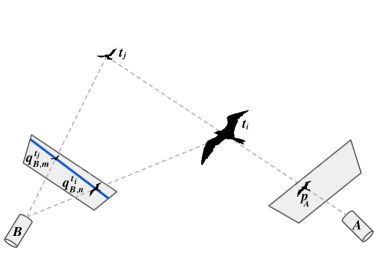
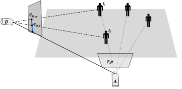
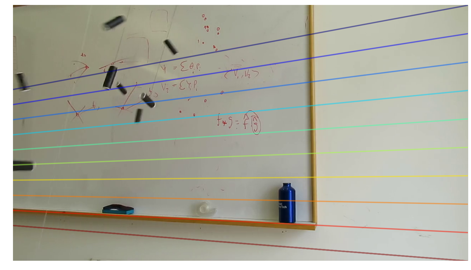
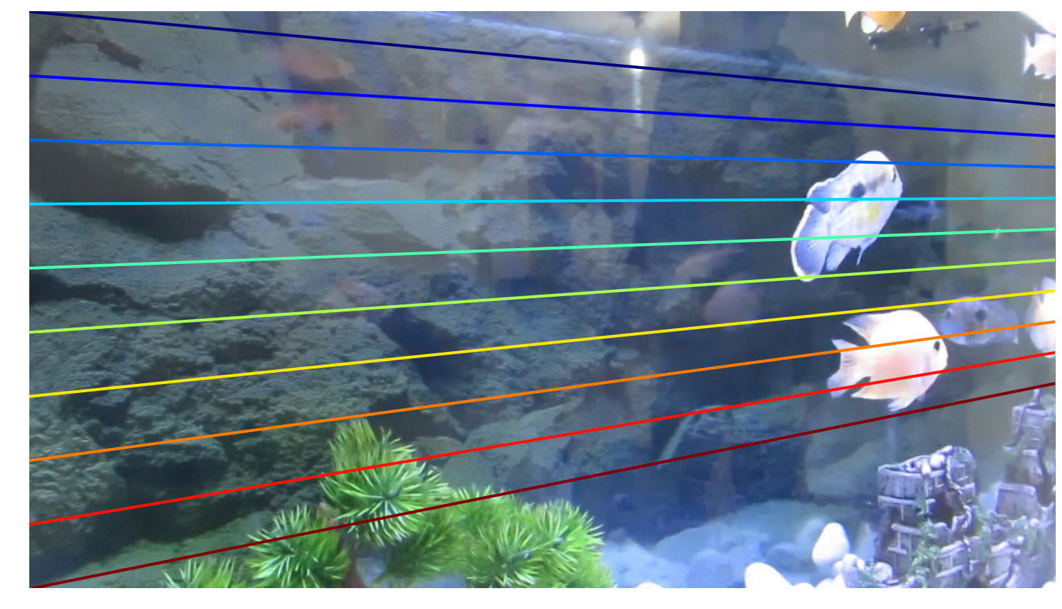
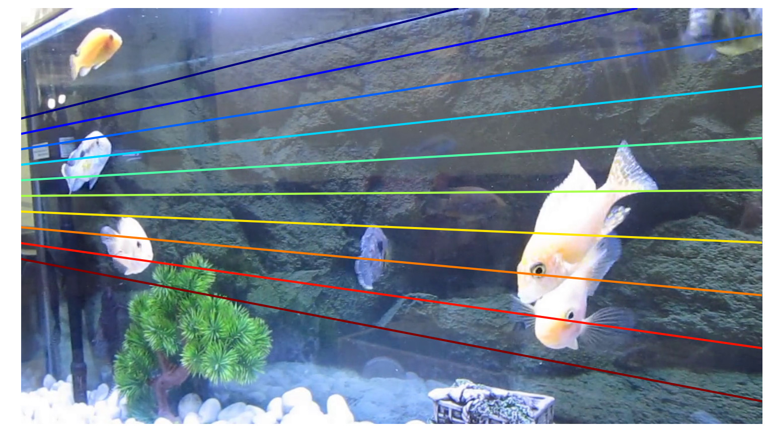
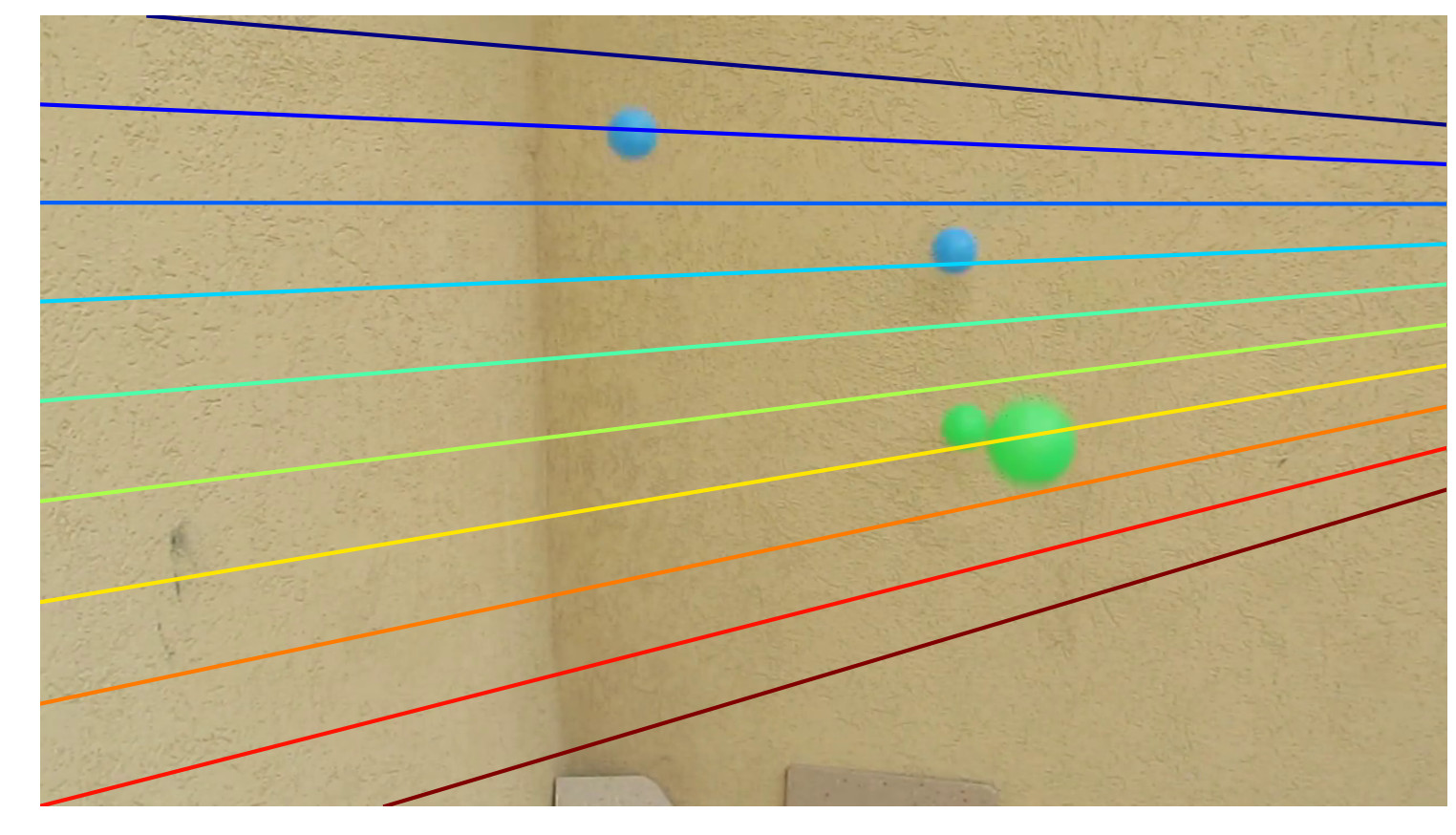
In this paper we propose a new method to compute the epipolar geometry from a video stream, by exploiting the following observation: For a pixel in Image , all pixels corresponding to in Image are on the same epipolar line. Equivalently, the image of the line going through camera ’s center and is an epipolar line in . Therefore, when cameras and are synchronized, the momentary images of two objects projecting to the same pixel, , in camera at times and , lie on an epipolar line in camera . Based on this observation we achieve fast and precise computation of epipolar lines.
Calibrating cameras based on our method of finding epipolar lines is much faster and more robust than previous methods.
1 Introduction
††footnotetext: This research was supported by the Israel Science Foundation and by the Israel Ministry of Science and Technology.The fundamental matrix is a basic building block of multiple view geometry and its computation is the first step in many vision tasks. This computation is usually based on pairs of corresponding points. Matching points across images is error prone, especially between cameras with very different viewpoints, and many subsets of points need to be sampled until a good solution is found. In this paper, we address the problem of robustly estimating the fundamental matrix from line correspondences in dynamic scenes.
The fundamental matrix is a homogeneous rank two matrix with seven degrees of freedom. The best-known algorithm for computing the fundamental matrix is the eight point algorithm by Longuet-Higgins [13] which was made practical by Hartley [7, 8], and is the heart of the Gold Standard algorithm [8]. The overall method is based on normalizing the data, solving a set of linear equations and enforcing the rank 2 constraint [15]. However, it suffers from decreased accuracy when the angle between the cameras becomes wide as corresponding points become dissimilar and hard to detect, making it unsuitable for very wide angles. In such cases, if videos of moving objects are available, the fundamental matrix can still be computed using motion cues.
Usually, the first step for calibrating cameras from moving objects is feature tracking, using e.g. deep features [1]. Khan and Shah[10] tracked features on a plane (people viewed from multiple surveillance cameras), and used their trajectories to compute a planar homography between the cameras. For this, they had to assume temporally synchronized cameras, long videos (minutes), and very particular movement patterns of the tracked objects. Our method shares only the first of these assumptions.
Following other papers based on motion [19, 3, 9] (and [2] for still images), we use epipolar lines instead of points to compute the fundamental matrix. The use of corresponding epipolar lines instead of corresponding points has a number of good attributes; a) The exponent in RANSAC execution time depends on the size of the minimal set needed to compute the model, which is no more than 3 for epipolar lines, as opposed to 7 for points, b) Line pairs can be filtered with motion barcodes even in very disparate views where points cannot. Indeed, three corresponding pairs of epipolar lines are enough to compute the fundamental matrix [8]. The epipolar lines in each image intersect at the epipole, and the one-dimensional homography between the lines can be recovered by the 3 line correspondences. The 3 degrees of freedom for the 1D homography, together with the 4 degrees of freedom of the epipoles, yield the 7 parameters needed to compute the matrix.
Sinha and Pollefeys [19] used the silhouette of a single moving object to find corresponding epipolar lines to calibrate a network of cameras. Ben-Artzi et al. [3] accelerated Sinha’s method using a similarity measure for epipolar lines based on motion barcodes defined in [4, 17]. This line motion barcode was also used in [9] to find corresponding epipolar lines and is the most relevant paper to ours. In that paper, they found corresponding epipolar lines by matching all pairs of lines between the images using the motion barcode. We propose to accelerate this process by drastically reducing the search space for matching epipolar lines, utilizing pixels which record multiple depths.
On top of that, we use centroids of detected foreground areas as a proxy for an object’s location, following Meingast et al. [16] who used it as features for correspondences of tracks from a multi-target tracking algorithm. Theoretically, estimating geometric properties based on fuzzy measurements such as areas resulting from foreground segmentation, or their centroids could be error prone. However, as shown by [16], and again by our experiments, this method is robust and accurate, and when followed by a global optimization step its accuracy can be further increased. We propose such a step to refine the epipole, by better approximating the intersection of the epipolar lines. To this end, we develop a general efficient algorithm that, given a set of lines, finds a point with the minimal sum of distances to all the lines ( metric), in addition to the usual sum of squared distances ( metric).
As in previous methods, we assume stationary cameras and that moving objects have been extracted by background subtraction.
The contributions of this paper are: i) A novel algorithm to calibrate a pair of synchronized video cameras, based on motion barcodes with much smaller complexity compared to the state-of-the-art, while maintaining robustness and accuracy; ii) An epipole refinement procedure, which leads to more accurate camera calibration.
2 Motion Barcodes
Motion barcodes of lines are used in the case of synchronized stationary cameras recording a scene with moving objects. Following background subtraction we have a binary video, where “0” represents static background and “1” moving objects.
Given such a video of binary frames, the motion barcode of a given image line is a binary vector in where iff a moving object intersects in the frame, [3]. An example of a motion barcode is shown in Figure 1.

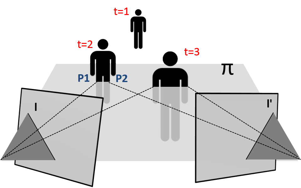
The case of a moving object seen by two cameras is illustrated in Figure 2. If the object intersects the epipolar plane at frame , and does not intersect the plane at frame , both motion barcodes of lines and will be at frames respectively. Corresponding epipolar lines therefore have highly correlated motion barcodes, and the similarity measure between motion barcodes and is their normalized cross correlation [4].
3 Epipolar Lines
Corresponding epipolar lines are projections of epipolar planes, 3d planes that go through both camera centers. Pixels are projections of 3d rays through a camera center.
The search for corresponding epipolar lines in this paper is based on finding two different corresponding pixels in camera to a given pixel in camera . These two correspondences are necessarily on an epipolar line in the other camera. The cue for matching, if there is no auxiliary information, such as tracking, color, or reliable shape features, is co-temporal movement.
The following notation is used throughout the paper:
pixels
pixel imaged in camera at time
line between pixels and in camera
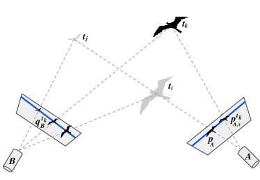
Given a pixel imaged at times and , the corresponding pixels in Image , and are on the epipolar line, . Likewise, is a point on the epipolar line in image corresponding to the epipolar line in image .
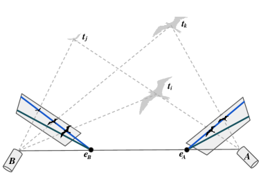
The algorithm for finding pairs of corresponding epipolar lines has two main steps, (i) finding two different pixels in corresponding to a single pixel in , which results in a single epipolar line in and (ii) finding the corresponding epipolar line in , chosen from the pencil of lines through , which gives a corresponding pair of epipolar lines.
4 Algorithm
Our algorithm assumes background subtraction, and the only pixels we are interested in are the centers of mass of the detected moving objects. Therefore, for the rest of this paper, whenever we refer to a pixel it is assumed to be the center of mass of some moving object.
4.1 Point to Line
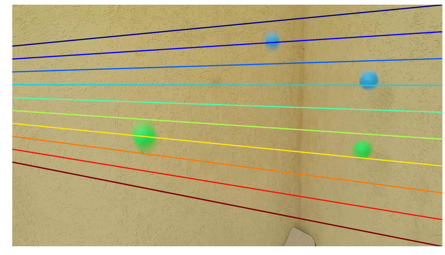
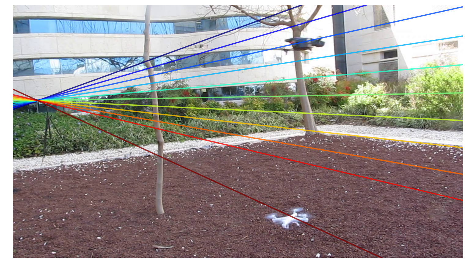
For two frames in camera taken at times , and both containing the same pixel , we will look at all the pixels from these frames in camera , that is: and . Each ordered pair of pixels from the two frames gives an epipolar line candidate, and let be the set of all such lines, see Figure 3(a).
We now turn to find a matching line in for each candidate line in . For each , we attempt to find a third frame at time containing an additional pixel on . Such points usually exist in real videos. Now for such a , let be all the pixels in camera at time , and let be the lines in camera between and every such pixel, that is: , Figure 3(b). Finally, the line whose motion barcode has the highest normalized cross-correlation to our ’s barcode is chosen as ’s partner, and partners with normalized cross-correlation above a certain threshold are considered a pair of possible corresponding epipolar lines. In order to proceed to the next stage we need at least two pairs of candidate lines.
It is worth noting that although the correspondence relation between each pair of line candidates is itself symmetric with respect to the roles of cameras and , the process producing these pairs is not; reversing the roles of cameras and and running the same algorithm as above, may result in a different set of pairs of line candidates.
When there is enough motion in the scene, using pixels in that have 3 or more corresponding pixels in produces much better matches, and with far fewer false positives, since we can easily check if all these correspondences in are indeed co-linear. In such cases our algorithm runs much faster and is more robust; first, because we have fewer line candidates to check, and second, the chances of coincidentally having 3 pixels on the same line in 3 given frames are very low, thereby reducing the probability of errors.
4.2 Third Line
We use RANSAC to estimate the location of the epipoles. We sample two pairs of putative corresponding epipolar lines from the previous step, and , with the probability to sample a pair proportional to its matching score (normalized cross-correlation). The intersection of the pairs and suggests two epipoles locations, and respectively (Figure 4). In order to compute the 1D line homography, a third pair of lines is required. If such a pair is available we skip the following step and move directly to the validation step. Otherwise, we pick a random frame and connect all foreground objects to the epipoles with lines , and . The third correspondence is found by matching the barcodes of lines from with those of and taking the best candidate to be the third pair.
These three pairs determine the 1D line homography, which together with the epipoles is sufficient to compute the fundamental matrix.
4.3 Validation
The validation step is carried out for each RANSAC iteration, to evaluate the quality of the estimated epipoles and homography. Similarly to [2], we compute the 1D line homography between the 3 pairs of lines, sample uniformly 10 lines from the pencil around , transform them to the pencil around , and compute the barcode cross-correlation between the 10 pairs of lines. The epipoles and homography with the highest score are used to compute the fundamental matrix between the cameras.
5 Extensions
5.1 Planar motion
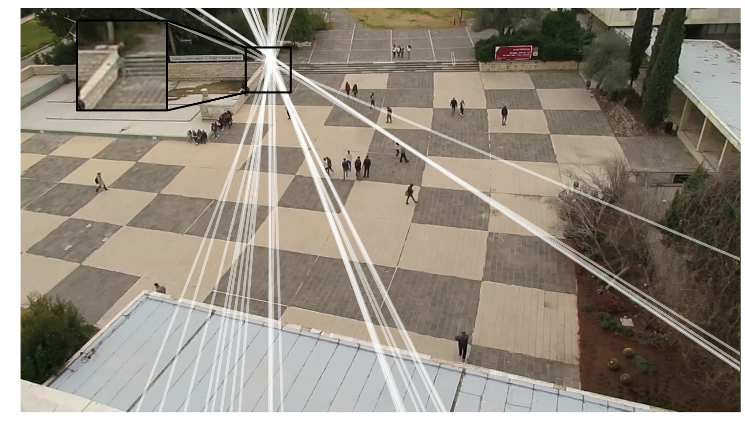
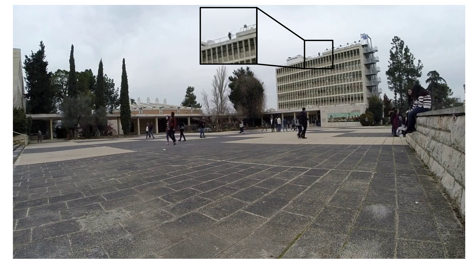
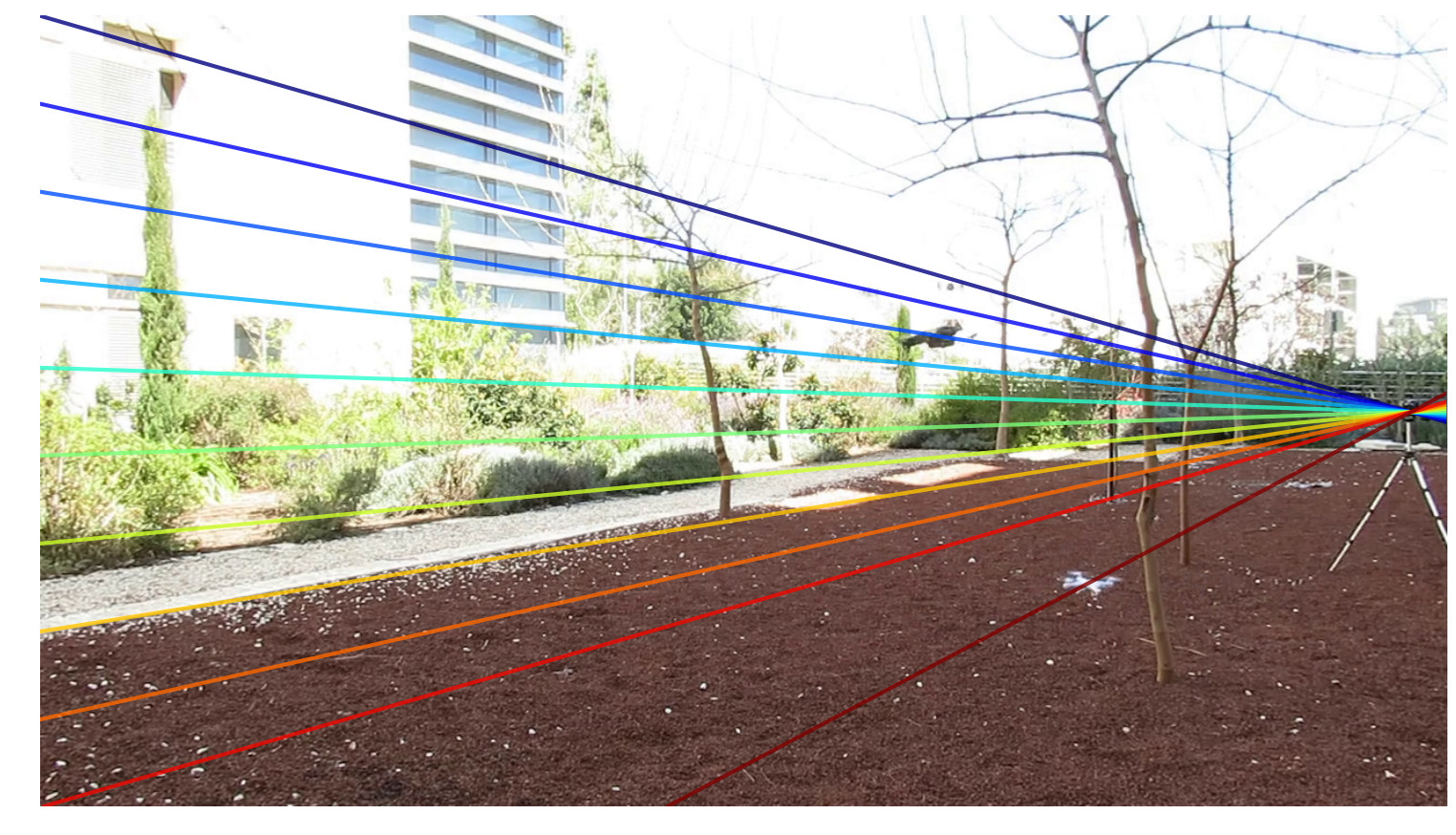
Our algorithm does not work on pure planar motion due to the major requirement of two distinctive objects having different depths on a single ray from the camera. However, in the special configuration of one camera on the plane and the other off it, the location of the epipole in the off-plane camera frame may be recovered. In this variant of the algorithm, We compute candidate lines in for a point , where the on-plane camera plays the role of camera . We exploit the following facts, (i) there is no motion outside the plane, and (ii) camera is off the plane. As a consequence, all the motion visible on the epipolar line through is concentrated around (see Figure 5). We then sample ’s barcode from a disc around it, instead of sampling from a line, and use NCC with the barcodes of . The one with highest score is kept. We only recover epipolar lines in , which is not enough to run the validation step, to choose the correct epipole among all intersections of lines. Instead, we ignore all lines whose matching score with their corresponding point falls under a certain threshold, and vote for the epipole by maximal consensus voting among the remaining lines. This step is carried out using RANSAC, where two lines are drawn in every iteration, their intersection yields the candidate epipole, and the number of lines which agree with the epipole is counted. The candidate with the maximal set of inliers is chosen as the epipole. A common definition for inliers in this scenario is the one introduced by [9], which we adopt for our controlled experiments. That being said, when the epipole is inside the image boundaries a simpler approach which works well is measuring whether the perpendicular distance between the epipole and a line is below a certain threshold. As a side effect, this process allows camera to be wide-angle with extreme lens distortion, a useful attribute for such a scenario (see the scene coverage of the planar camera in Figure 6). We do not measure image lines in , thus lens distortion does not affect the computations, because from the point of view of camera we are only interested in rays through pixels, and those are not altered by lens distortion. This side effect may even benefit accuracy, which is improved by incorporating the increased amount of epipolar lines in imaged in , and possibly larger angles between pairs of lines.
5.2 Static objects
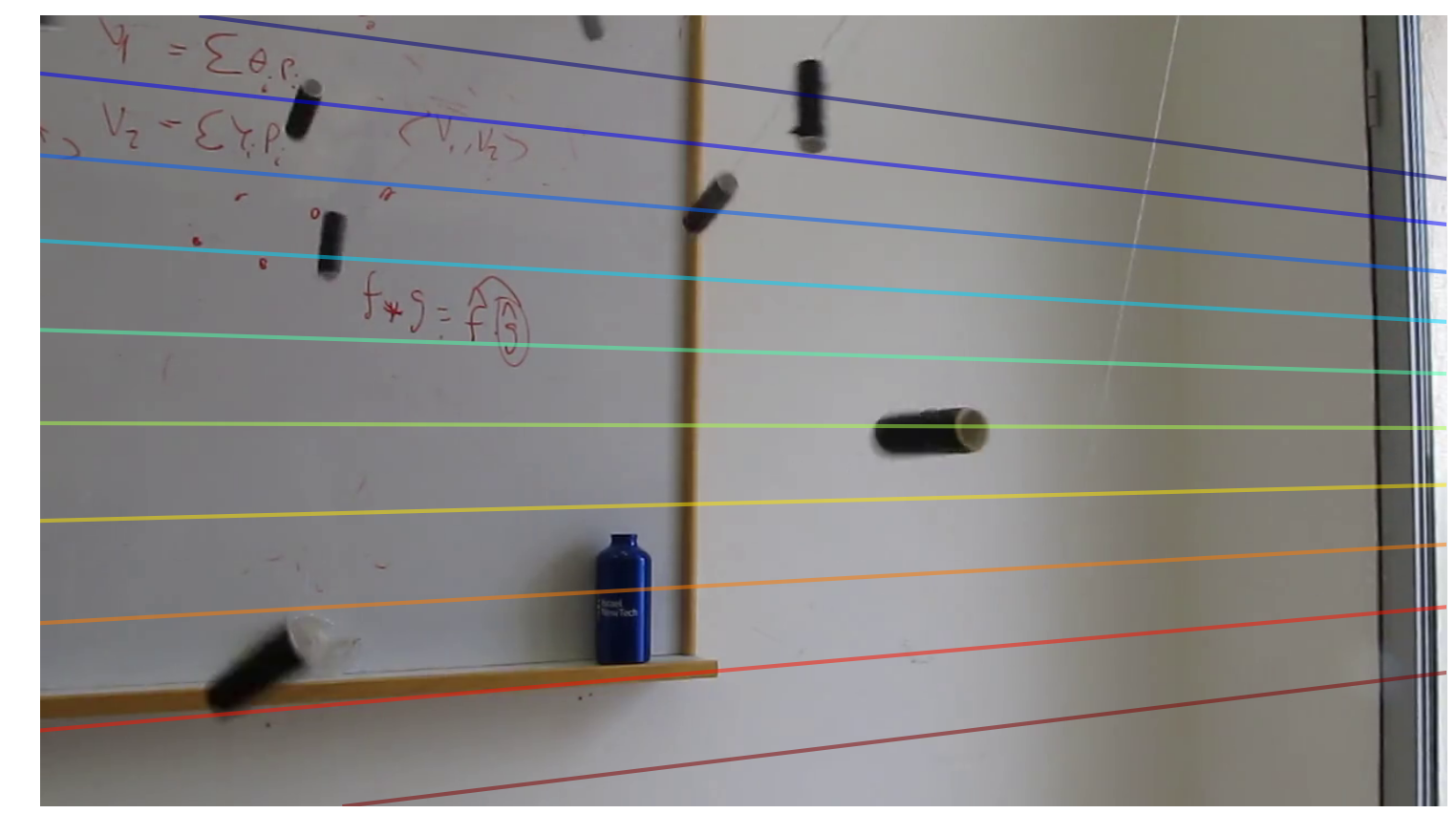
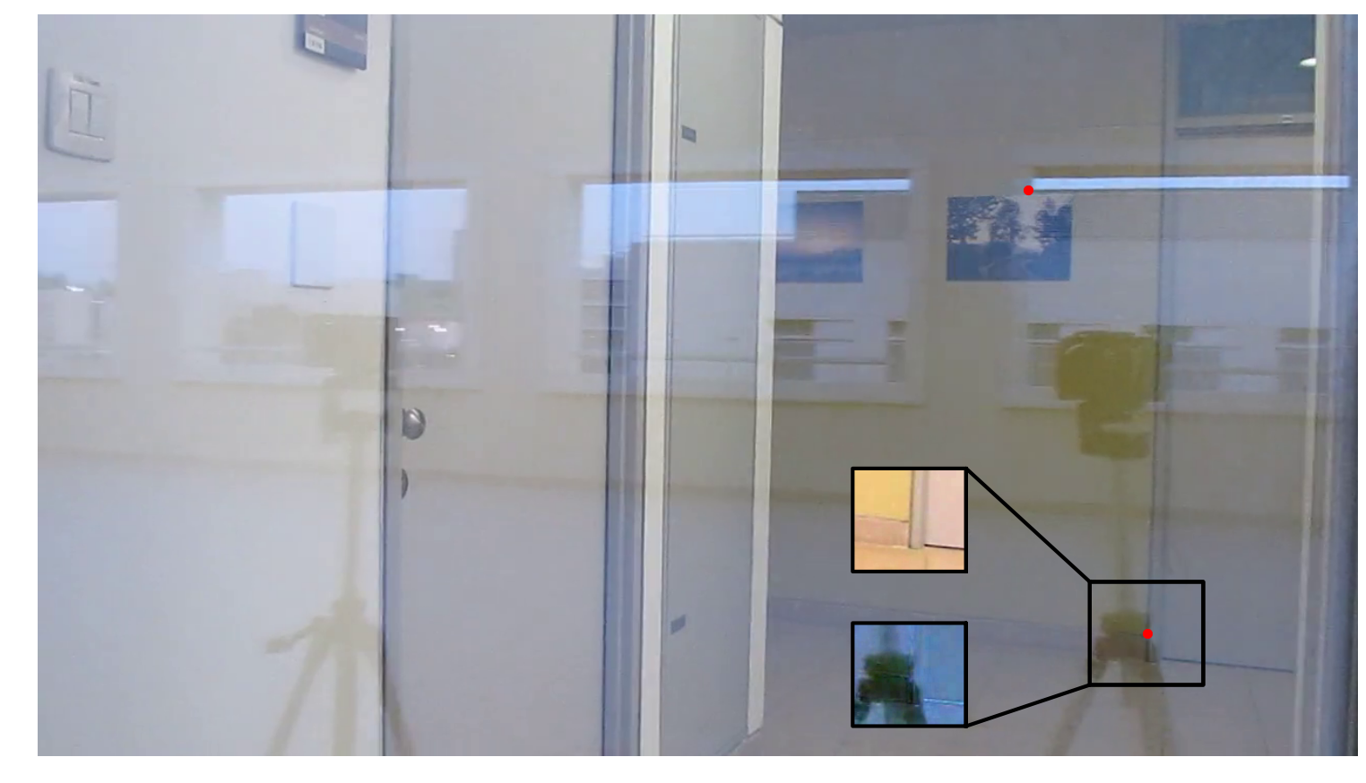
In certain cases, features of multiple objects projected to the same point may be extracted. A dynamic object can occlude a static one, for which a different kind of feature (e.g. SIFT[14]) can be detected, or the scene can even be fully static with multiple objects detected at the same image point, such as semi transparent surfaces. Various algorithms exist to separate reflections from transmitted light (for example [11, 12, 18]). Two features extracted from the separated layers at the same location, with their matched corresponding points on different locations in the other camera, will produce an epipolar line. See example in Figure 11.
5.3 Coupling with other features
In addition to motion barcodes other types of features can guide the matching process. For example, two objects imaged on having certain colors (identifiable from other viewing points) will constrain the search in for objects with matching colors. More complex features such as deep features could be used, for example in a natural scene with a large number of moving objects, we can isolate one kind of moving object, e.g. butterflies, and process only their locations.
6 Epipole Refinement
We refine the estimated epipoles and epipolar geometry using inlier lines. Line pairs are defined as inliers if they agree with the epipoles via the measure Kasten et. al introduced in [9]. They measure the area between a given line and a true epipolar line intersecting it at the central vertical line of the image. We use the same threshold of 3 times the width of the frame, as the threshold below which the line is an inlier. For the refinement process we do not have the true epipoles, but use instead our estimated ones from the validation process. Note that the inlier percentage in the controlled experiments in Tables 1 and 2 is computed using the ground truth epipoles, in order to get the true number of inliers.
Point-line distance
The perpendicular (signed) distance between a line and a point can be expressed as a dot product , where is normalized such that , and is normalized such that [6].
refinement
This is simply least-squares, used to compute a refined epipole minimizing
| (1) |
given the inlier lines . The complexity is linear in the number of lines.
refinement
The loss
| (2) |
is a convex function, and is linear inside each of the cells of the line arrangement, hence its global minimum is obtained on an intersection of two of the lines, which is a vertex of a cell. In general, in the presence of outliers, refinement is more robust than .
Iterative minimization
The complexity of using Brute Force to find is where is the number of lines, since there are intersections, requiring calculations each. We propose an efficient iterative algorithm to find in . First, we compute the arrangement of the lines, a process that can be done by topological sweeping in [5]. Next, we pick an intersection at random, and split the lines to two sets and , composed of the lines with and , respectively. We get
| (3) |
Moving to a neighbor of might cause a line to switch between and , as the line is incident to but not to , i.e. and . As a consequence, after moving from to (or vice versa) if necessary, and updating the sums, we can efficiently compute . At each step, updating the sum requires changing the sums by adding/subtracting at most one line, thus taking . We examine the neighbors of , and move to the one with lowest loss. We traverse the arrangement until the minimal point is found, visiting at most intersections, where at each we spend computations.
Fundamental matrix refinement
Our refinement algorithm works as follows; (i) Compute refined epipole locations based on inlier pairs of lines. Recall that since we do not know the true epipoles we rely on our estimated epipoles to identify inlier lines. (ii) Perform RANSAC iterations similar to the ’third line’ step (section 4.2), but in which we sample all three frames at every iteration. In each of the frames we connect lines from the pixels to the refined epipoles, and take the best matching pair of lines. (iii) The three best pairs (one pair of lines for each frame) are sufficient to compute the epipolar geometry, which gets a score using the validation process described in section 4.3. To overcome errors introduced by outlier lines, we compare the validation score of the initial fundamental matrix with those computed using refinement and refinement. The final epipoles and homography are those with the highest validation score.
|
|
|
|
|
|
|||||||
|---|---|---|---|---|---|---|---|---|---|---|---|---|
|
|
|
|
|
|
|||||||
| Kasten et. al [9] |
|
|
|
|
|
|
||||||
| Ours |
|
|
|
|
|
|
|
|
|
|
|
|
|||||||
|---|---|---|---|---|---|---|---|---|---|---|---|---|
|
|
|
|
|
|
|||||||
| Kasten et. al [9] |
|
|
|
|
|
|
||||||
| Ours |
|
|
|
|
|
|
7 Experiments
We evaluated our algorithm on real and simulated video streams. Since this approach is novel, there are no existing suitable real datasets with ground truth calibration.
The authors of [9] provided us with their synthetic datasets cubes and thin cubes, comprised of 5 and 7 cameras, respectively. We adopted their area measure and used the same threshold for defining inliers.
Our algorithm shares with theirs the RANSAC procedure, whereas the acceleration in our algorithm stems mostly from the first step in which we find putative corresponding epipolar line pairs. We reimplemented their method with our barcode sampling and matching, to allow a fair comparison. We tested our method on all camera pairs from both datasets (see Tables 1 and 2 for quantitative comparison with state of the art). Kasten et al. [9] sampled a constant number of line barcodes, spaced equally on the image boundaries. On average, their number of barcodes is 20x-75x the amount of barcodes we sample. The tables also show the percent of inliers among the line candidates, which are all candidates in our method, and the 1000 line pairs with top matching score in [9]. Our average Symmetric Epipolar Distance (SED) is comparable to [9], and even outperforms their method when applying global refinement, while reducing the time complexity by two orders of magnitude. The run time increase caused by refinement is negligible, and the increase due to refinement depends on the actual number of lines taken into calculation, but it never took more than a second to optimize.
The code was written in Python, and all experiments were conducted on a standard desktop computer with no GPU acceleration.
7.1 Real videos
To validate our method on real video examples, we captured several scenes with various types of motion.
Figure 6 shows an example from a real video with planar motion. A wide angle camera (GoPro Hero 3+) is mounted at a height of about a meter above ground and facing towards a busy square (right image). Another camera, , captured the same scene from a typical surveillance angle from a nearby roof (left image).
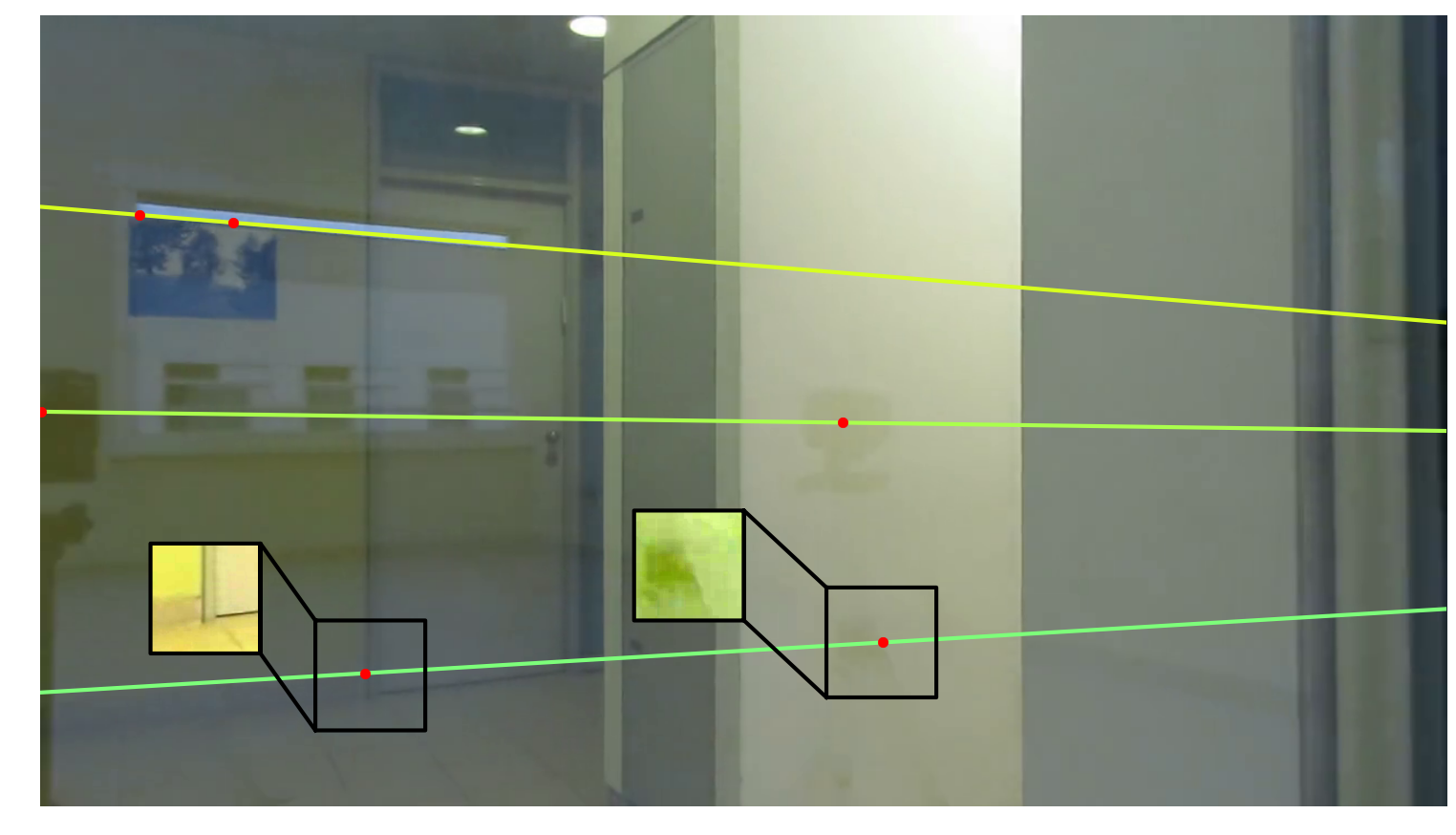
An example of images of a static scene with a semi transparent surface is shown in Figure 11. Behind the flat window, part of a corridor with two doors and a painting on the wall is visible. The reflection on the glass consists of the two cameras with tripods, and the buildings behind. The difference in colors between the cameras is due to different white balance. The two red dots marked on the left image () are points where two corner points were detected on different surfaces (one behind the glass and one reflected on it), and the two layers have been separated and shown individually. The two black boxes show a detected corner point on a door and a point on the tripod of camera . The same points are marked with red dots on the right image (). Since the reflecting surface is flat, the virtual location of the reflected tripod is the same for and . Thus, its projection on must lie on the same epipolar line as the corner of the door. A second line is obtained by applying the same to the second marked point in , and their intersection yields the epipole. For visualization, the reflections of the two camera centers, which of course share an epipolar line, have also been marked and connected by a line.
8 Conclusion
We introduced a method for finding corresponding epipolar lines from multiple pixel correspondences in one camera to a single pixel in the other. We conducted experiments with real and synthetic videos, where our method was shown to calibrate cameras with state of the art accuracy while consuming far less computation time, compared to existing methods on a standard dataset.
Acknowledgements
The authors would like to thank Or Sharir and Uri Karniel for their help in conducting the experiments.
 |
 |
| (a) | (b) |
 |
 |
| (a) | (b) |
References
- [1] G. Amato, F. Falchi, C. Gennaro, and F. Rabitti. Similarity Search and Applications: 9th International Conference, SISAP, chapter YFCC100M-HNfc6: A Large-Scale Deep Features Benchmark for Similarity Search, pages 196–209. Springer International Publishing, Cham, 2016.
- [2] G. Ben-Artzi, T. Halperin, M. Werman, and S. Peleg. Epipolar geometry based on line similarity. In ICPR, 2016.
- [3] G. Ben-Artzi, Y. Kasten, S. Peleg, and M. Werman. Camera calibration from dynamic silhouettes using motion barcodes. In CVPR’16, 2016.
- [4] G. Ben-Artzi, M. Werman, and S. Peleg. Event retrieval using motion barcodes. In ICIP’15, pages 2621–2625, 2015.
- [5] H. Edelsbrunner and L. J. Guibas. Topologically sweeping an arrangement. In Proceedings of the eighteenth annual ACM symposium on Theory of computing, pages 389–403. ACM, 1986.
- [6] I. D. Faux and M. J. Pratt. Computational geometry for design and manufacture. Ellis Horwood Ltd, 1979.
- [7] R. Hartley. In defense of the eight-point algorithm. IEEE Trans. PAMI, 19(6):580–593, 1997.
- [8] R. Hartley and A. Zisserman. Multiple view geometry in computer vision. Cambridge university press, 2003.
- [9] Y. Kasten, G. Ben-Artzi, S. Peleg, and M. Werman. Fundamental matrices from moving objects using line motion barcodes. In European Conference on Computer Vision, pages 220–228. Springer International Publishing, 2016.
- [10] S. Khan and M. Shah. Consistent labeling of tracked objects in multiple cameras with overlapping fields of view. IEEE Transactions on Pattern Analysis and Machine Intelligence, 25(10):1355–1360, 2003.
- [11] A. Levin and Y. Weiss. User assisted separation of reflections from a single image using a sparsity prior. IEEE Transactions on Pattern Analysis and Machine Intelligence, 29(9), 2007.
- [12] Y. Li and M. S. Brown. Single image layer separation using relative smoothness. In Proceedings of the IEEE Conference on Computer Vision and Pattern Recognition, pages 2752–2759, 2014.
- [13] H. Longuet-Higgins. A computer algorithm for reconstructing a scene from two projections. Nature, 293:133–135, 1981.
- [14] D. G. Lowe. Distinctive image features from scale-invariant keypoints. International journal of computer vision, 60(2):91–110, 2004.
- [15] Q.-T. Luong and O. Faugeras. The fundamental matrix: Theory, algorithms, and stability analysis. IJCV, 17(1):43–75, 1996.
- [16] M. Meingast, S. Oh, and S. Sastry. Automatic camera network localization using object image tracks. In Computer Vision, 2007. ICCV 2007. IEEE 11th International Conference on, pages 1–8. IEEE, 2007.
- [17] D. Pundik and Y. Moses. Video synchronization using temporal signals from epipolar lines. In ECCV’10, pages 15–28. Springer, 2010.
- [18] Y. Shih, D. Krishnan, F. Durand, and W. T. Freeman. Reflection removal using ghosting cues. In Proceedings of the IEEE Conference on Computer Vision and Pattern Recognition, pages 3193–3201, 2015.
- [19] S. Sinha and M. Pollefeys. Camera network calibration and synchronization from silhouettes in archived video. IJCV, 87(3):266–283, 2010.