The world of long-range interactions: A bird’s eye view

Abstract

In recent years, studies of long-range interacting (LRI) systems have taken centre stage in the arena of statistical mechanics and dynamical system studies, due to new theoretical developments involving tools from as diverse a field as kinetic theory, non-equilibrium statistical mechanics, and large deviation theory, but also due to new and exciting experimental realizations of LRI systems. In the first, introductory, Section 1, we discuss the general features of long-range interactions, emphasizing in particular the main physical phenomenon of non-additivity, which leads to a plethora of distinct effects, both thermodynamic and dynamic, that are not observed with short-range interactions: Ensemble inequivalence, slow relaxation, broken ergodicity. In Section 2, we discuss several physical systems with long-range interactions: mean-field spin systems, self-gravitating systems, Euler equations in two dimensions, Coulomb systems, one-component electron plasma, dipolar systems, free-electron lasers. In Section 3, we discuss the general scenario of dynamical evolution of generic LRI systems. In Section 4, we discuss an illustrative example of LRI systems, the Kardar-Nagel spin system, which involves discrete degrees of freedom, while in Section 5, we discuss a paradigmatic example involving continuous degrees of freedom, the so-called Hamiltonian mean-field (HMF) model. For the former, we demonstrate the effects of ensemble inequivalence and slow relaxation, while for the HMF model, we emphasize in particular the occurrence of the so-called quasistationary states (QSSs) during relaxation towards the Boltzmann-Gibbs equilibrium state. The QSSs are non-equilibrium states with lifetimes that diverge with the system size, so that in the thermodynamic limit, the systems remain trapped in the QSSs, thereby making the latter the effective stationary states. In Section 5, we also discuss an experimental system involving atoms trapped in optical cavities, which may be modelled by the HMF system. In Section 6, we address the issue of ubiquity of the quasistationary behavior by considering a variety of models and dynamics, discussing in each case the conditions to observe QSSs. In Section 7, we investigate the issue of what happens when a long-range system is driven out of thermal equilibrium. Conclusions are drawn in Section 8.

1 Introduction: General considerations

In this Section, we discuss the generalities of long-range interacting systems. A detailed discussion, with extensive lists of references, may be found in several recent articles and books, see Refs. [1, 2, 3, 4, 5, 7, 6, 8]. More recent works discussed in the later parts of this article are covered in Refs. [26, 27, 28, 30, 31, 23, 24, 25, 32, 33, 34, 35].

Long-range interacting (LRI) systems are those in which the two-body interparticle potential decays at large separation $r$ as

$$V(r)\sim\frac{J}{r^{\alpha}};~{}0\leq\alpha\leq d,$$ (1)

where $d$ is the dimension of the embedding space, and $J$ is the coupling strength . The range of allowed values of the decay exponent $\alpha$ implies that the energy per particle, $\varepsilon$, scales super-linearly with the system size. This feature is easily demonstrated by considering the example of a particle placed at the center of a hypersphere of radius $R$ in $d$ dimensions, with the other particles homogeneously distributed with a mass density $\rho$. For such a system, considering the interaction potential (1), the energy per particle is given as

$$\varepsilon=\int_{\delta}^{R}{\rm d}^{d}r~{}\rho\frac{J}{r^{\alpha}}=\frac{\rho J\Omega_{d}}{d-\alpha}\left[R^{d-\alpha}-\delta^{d-\alpha}\right],$$ (2)

where $\delta\to 0$ is a short distance cut-off introduced to exclude the contribution to the energy due to particles located in a small neighborhood of radius $\delta$, and is motivated by the need to regularize the divergence of the potential (1) at short distances. In Eq. (2), $\Omega_{d}$ denotes the angular volume in $d$ dimensions. From the equation, it follows that as $R$ is increased, the energy $\varepsilon$ remains finite for $\alpha>d$, implying thereby the linear scaling of the total energy $E$ with the volume $V\sim R^{d}$, thus making the system extensive. These systems are called short-range interacting systems. On the other hand, for our allowed values of $\alpha$, the energy $\varepsilon$ scales with the volume as $\varepsilon\sim V^{1-\alpha/d}$ (the energy scales logarithmically with $V$ in the marginal case $\alpha=d$), thereby implying a super-linear scaling of the total energy of LRI systems with $V$, as $E\propto V^{2-\alpha/d}$. The LRI systems are thus generically non-extensive. For such systems, on computing the free energy $F\equiv E-TS$, with $T$ being the intensive temperature and $S$ being the entropy that typically scales linearly with the volume, $S\sim V$, we find due to the super-linear scaling of $E$ with $V$ that the thermodynamic properties are dominated by the energy. In particular, the equilibrium state of a mechanically isolated LRI system at constant temperature, obtained by minimizing $F$, corresponds to the one with the minimum energy, that is, the ground state, allowing for no thermal fluctuations. Of course, in reality, there ought to be a competition between the energy and the entropy contributions to the free energy in order to have such phenomena as phase transitions that are known to occur in LRI systems. A way out from this energy dominance consists in scaling the coupling constant as

$$J\to\frac{J}{V^{1-\alpha/d}},$$ (3)

thereby making the energy extensive in the volume. Note that this is just a “mathematical trick” (Kac’s trick) to properly study LRI systems within the framework of equilibrium statistical mechanics that exists for short-range ones, and does not correspond to any physical effect. Indeed, no interaction whose strength changes on varying the volume is known to occur. Applying this trick, one can obtain the free energy per particle, and then revert to the actual physical description by scaling back the coupling constant. An equivalent alternative to Kac’s trick, which still allows for an effective competition between the energy and the entropy contribution to the free energy, consists in rescaling the temperature as

$$T\to\frac{T}{V^{\alpha/d-1}}.$$ (4)

Beyond the rescaling procedures discussed above, which were implemented to obtain a meaningful large-volume limit for LRI systems and competing energy and entropy contributions to the free energy, let us illustrate how such a competition may actually occur in nature, by considering a relevant LRI system in the arena of astrophysics, namely, that of globular clusters, see Fig. 1. These clusters are gravitationally bound concentrations of $N\sim 10^{4}-10^{6}$ stars that are spread over a volume that has a diameter ranging from several tens to about $200$ light years (1 light year = $9.4\times 10^{15}$ m). For a typical globular cluster (M2), one has $N=1.5\times 10^{5}$, $R=175$ light years, and total mass $M=2\times 10^{30}$ Kg. An order-of-magnitude estimate of energy and entropy may be done as follows:

$$E=\frac{GN^{2}M^{2}}{R},~{}S=k_{B}N\implies\frac{E}{S}\sim\frac{GNM^{2}}{k_{B}R}\sim 1.7\times 10^{60}~{}{\rm K},$$ (5)

where $G$ is the gravitational constant, and $k_{B}$ is the Boltzmann constant. To such an extremely high temperature as $\sim 10^{60}$ K, one can associate a velocity by invoking energy equipartition (neglecting interactions), as $v=\sqrt{\frac{3k_{B}T}{M}}\simeq 5.9$ Km/s. Typical star velocities indeed range between a few Km/s to about $100$ Km/s. Thus, for systems such as these for which the temperature is high enough, the energy, although super-linear in volume ($E\sim V^{5/3}$), can effectively compete with the entropy contribution to the free energy.

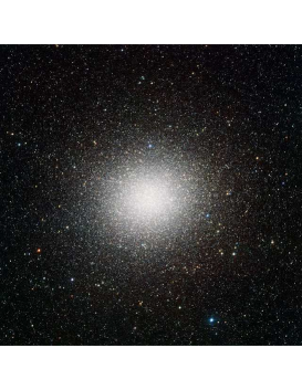
Figure 1: Spherically symmetric mass distribution of stars in a globular cluster.

Let us now make an important remark: Although Kac’s trick allows to obtain an energy that is extensive in the volume, it is not necessarily additive (additivity implies extensivity, but not the converse). A simple example will illustrate the point. Consider the well-studied Curie-Weiss model of magnetism, with the Hamiltonian given by

$$H_{\rm CW}=-\frac{J}{2N}\sum_{1\leq i<j\leq N}\sigma_{i}\sigma_{j},$$ (6)

where $\sigma_{i}=\pm 1$ are spin variables occupying the sites $i$ of a lattice. The model mimics a mean-field system (every spin interacting with every other with the same strength), which may be considered as the $\alpha\to 0$ limit of the potential (1). Being a mean-field system, one does not need to specify the structure of the underlying lattice, excepting to mention that every site is connected to every other. In the Hamiltonian (6), the coupling strength has been rescaled by using Kac’s trick, so that the energy is extensive in the number of spins given by $N$. Let us consider a macrostate with zero total magnetization: $M\equiv\sum_{i=1}^{N}\sigma_{i}=0$, which is composed of $N/2$ spin-$(+1)$ sites and $N/2$ spin-$(-1)$ sites, see Fig. 2. Since the energy is proportional to the square of magnetization (see Eq. (6)), the total energy of the system is $E_{1+2}=0$. However, the energy of the two parts, namely, $E_{1}=E_{2}=-J/8N$, does not vanish, and, therefore, $E_{1+2}\neq E_{1}+E_{2}$.

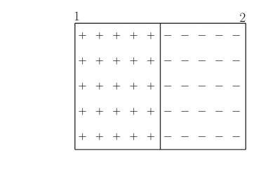
Figure 2: Non-additivity in the extensive Curie-Weiss model: A zero magnetization macrostate of the Curie-Weiss system, Eq. (6), constituted by $N/2$ up-spins in domain 1 and $N/2$ down-spins in domain 2. Here, an up-spin is denoted by a $+$ sign and a down-spin by a $-$ spin.

As it will emerge in the rest of this article, the violation of additivity will be crucial in determining both thermodynamic and dynamic properties of LRI systems, making them quite distinct from short-range ones. This point will be demonstrated by considering several illustrative examples in the later parts of the paper. As a warm-up, we may mention that a violation of additivity implies a violation of convexity of the domain of accessible macrostates of an LRI system, for example, a magnetic one in the magnetization ($M$) - energy ($E$) plane. An example of such a violation is shown in Fig. 3, where the boundary of the region of accessible macrostates is shown to have the shape of a bean. For short-range systems for which additivity is satisfied, standard thermodynamics implies that all states satisfying

$$E=\lambda E_{1}+(1-\lambda)E_{2},~{}M=\lambda M_{1}+(1-\lambda)M_{2},~{}0\leq\lambda\leq 1$$ (7)

must occur at the macroscopic level; this is in general not the case for LRI systems, and may imply a violation of ergodicity in the microcanonical ensemble. For example, the states $(M_{1},E_{1})$ and $(M_{2},E_{2})$ in Fig. 3 are not connected by any continuous energy-conserving dynamics.

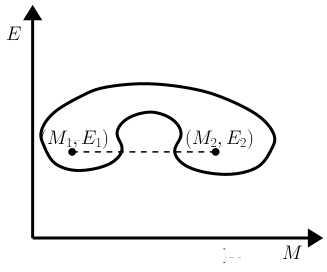
Figure 3: Non-convex shape of the region of accessible macrostates in the magnetization-energy plane for a magnetic LRI system. The states $(M_{1},E_{1})$ and $(M_{2},E_{2})$ are not connected by any continuous energy-conserving dynamics.

On account of the violation of additivity, one should exercise caution in discussing equilibrium properties of LRI systems using the canonical ensemble whose derivation from the microcanonical ensemble relies on holding of additivity. Let us briefly recall the derivation. The microcanonical partition function for a system of $N$ particles contained in a volume $V$ in $d=3$ dimensions is given by

$$\Omega(E,V,N)\propto\int{\rm d}^{3N}q{\rm d}^{3N}p~{}\delta(E-H(p,q)),$$ (8)

where $(q,p)$ are the canonically conjugate variables, and $H$ is the Hamiltonian. The entropy is defined via

$$S(E,V,N)=k_{B}\ln\Omega(E,V,N),$$ (9)

where an energy scale should be included in the logarithm to make its argument dimensionless. In deriving the canonical ensemble for a short-range system, one considers an isolated macroscopic system with energy $E$ that is composed of a “small” part (the subsystem of interest) with energy equal to $E_{1}$, volume equal to $V_{1}$ and number of particles equal to $N_{1}$, and a “large” part that plays the role of a ”bath”, with energy equal to $E_{2}\gg E_{1}$, volume equal to $V-V_{1}\gg V_{1}$ and number of particles equal to $N-N_{1}\gg N_{1}$. The additivity of energy implies that one has $E_{2}=E-E_{1}$, so that the probability distribution $p(E_{1})$ that the “small” system has energy $E_{1}$ is given by

$$p(E_{1})\propto\Omega_{2}(E-E_{1},V-V_{1},N-N_{1}).$$ (10)

Using the definition of entropy and a Taylor expansion, one gets

$$p(E_{1}) = \exp\left[S_{2}(E-E_{1})\right]$$ (11)

$$\approx \exp\left[S_{2}(E)-E_{1}\left.\frac{\partial S_{2}}{\partial E}\right|_{E}+\cdots\right]$$

$$\propto \Omega_{2}(E,V-V_{1},N-N_{1})\;e^{-\beta E_{1}},$$

where $S_{2}(E)\equiv S_{2}(E,V-V_{1},N-N_{1})$, and $\beta\equiv\left.\frac{\partial S_{2}}{\partial E}\right|_{E}$ is the inverse temperature: $\beta=1/(k_{B}T)$. Equation (11) is the usual canonical ensemble description for the energy distribution of the system of interest. In describing LRI systems, which we have shown to be generically non-additive so that the derivation leading to (11) does not hold, we will consider both the microcanonical description, Eq. (8), and the canonical one, Eq. (11). For the latter, however, we will adopt an alternative physical interpretation, namely, that of the system of interest in interaction with an external heat bath at temperature $T$ that induces stochastic fluctuations into the dynamics of the system.

Thermodynamic ensembles could be inequivalent for LRI systems [9, 10, 11, 12]: a macroscopic physical state that is realizable in one ensemble is not realized in the other. We now discuss this point. Ensemble equivalence in the thermodynamic limit is mathematically based on certain properties of the partition functions. The thermodynamic limit corresponds to considering simultaneously the limits $N\rightarrow\infty$, $E\rightarrow\infty$ and $V\rightarrow\infty$, such that one has $N/V\rightarrow n$ and $E/N\rightarrow\varepsilon$, where the particle density $n\geq 0$ and the energy per particle $\varepsilon$ are finite quantities. In this limit, the entropy per particle is given by

$$s(\varepsilon,n)\equiv\lim_{N\rightarrow\infty}\frac{1}{N}S(E,V,N).$$ (12)

The function $s(\varepsilon,n)$ is continuous, increasing with $\varepsilon$ at a fixed $n$, so that the temperature $T=\left(\partial s/\partial\varepsilon\right)^{-1}$ is a positive quantity. For short-range systems, $s(\varepsilon,n)$ turns out to be a concave function of $\varepsilon$ at a fixed $n$:

$$s\left(\lambda\varepsilon_{1}+(1-\lambda)\varepsilon_{2},n\right)\geq\lambda s(\varepsilon_{1},n)+(1-\lambda)s(\varepsilon_{2},n),$$ (13)

for any choice of $\varepsilon_{1}$ and $\varepsilon_{2}$, with $0\leq\lambda\leq 1$. The partition function in the canonical ensemble is given by

$$Z(\beta,V,N)\equiv\int{\rm d}q^{3N}{\rm d}p^{3N}~{}\exp\left[-\beta H(p,q)\right].$$ (14)

In the thermodynamic limit, the free energy per particle is obtained as

$$f(\beta,n)\equiv-\frac{1}{\beta}\lim_{N\rightarrow\infty}\frac{1}{N}\ln Z(\beta,V,N).$$ (15)

Moreover, at a fixed $n$, the function $\phi(\beta,n)\equiv\beta f(\beta,n)$ (the rescaled free energy) is concave in $\beta$. The equivalence between the microcanonical and the canonical ensemble is a consequence of the concavity of $\phi$ and $s$ and of the relation between these two functions given by the Legendre-Fenchel Transform (LFT). Indeed, one can easily prove that $\phi(\beta,n)$ is the LFT of $s(\varepsilon,n)$:

$$\phi(\beta,n)=\inf_{\varepsilon}\left[\beta\varepsilon-s(\varepsilon,n)\right],$$ (16)

and also the inverse LFT holds, since $s(\varepsilon,n)$ is concave in $\varepsilon$:

$$s(\varepsilon,n)=\inf_{\beta}\left[\beta\varepsilon-\phi(\beta,n)\right].$$ (17)

These relations prove ensemble equivalence, because for each value of $\beta$, there is a value of $\varepsilon$ that satisfies Eq. (16), and, conversely, for each value of $\varepsilon$, there is a value of $\beta$ satisfying Eq. (17). Figure 4 provides a visual explanation of the relation between $s$ and $\phi$ and of the correspondence between $\varepsilon$ and $\beta$. Note that at a first-order phase transition, the entropy has a constant slope in the energy range $[\varepsilon_{1},\varepsilon_{2}]$ (the phase coexistence region), resulting in a free energy with a cusp at the transition inverse temperature $\beta_{t}$, see Fig. 5.

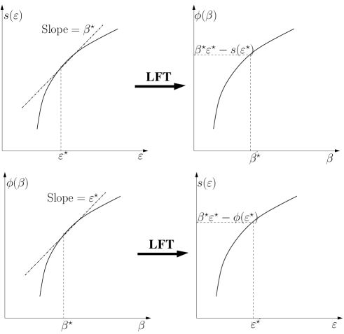
Figure 4: (Upper panel) Free energy from entropy by performing a Legendre-Fenchel transform. (Lower panel) Entropy from free energy by the same transform.

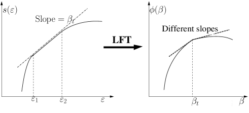
Figure 5: Relation between the entropy and the free energy at a first-order phase transition.

Now, for LRI systems, the entropy may be a non-concave function of the energy. In this case, the Legendre-Fenchel transform is no more involutive: if applied to the entropy, it returns the correct free energy. However, the Legendre-Fenchel transform of the free energy does not coincide with the entropy, but rather with its concave envelope; this is the basic feature causing ensemble inequivalence.

2 Examples of LRI systems

A wide class of LRI systems comprises $N$ interacting particles having the total potential energy

$$U(\vec{r}_{1},\dots,\vec{r}_{N})=\sum_{1\leq i<j\leq N}V(|\vec{r}_{i}-\vec{r}_{j}|)+\sum_{i=1}^{N}V_{e}(\vec{r}_{i}),$$ (18)

where $\vec{r}_{i}$ is the position of the $i$-th particle, $V$ is the interparticle potential and $V_{e}$ represents the potential energy due to an external field. In contrast to the continuum description of Eq. (18), long-range interactions may also be defined on a lattice (the Curie-Weiss model considered above was one such system), with the potential energy having the form

$$U({\bf q}_{1},\dots,{\bf q}_{N})=\sum_{1\leq i<j\leq N}C_{ij}V({\bf q}_{i},{\bf q}_{j})+\sum_{i=1}^{N}V_{e}({\bf q}_{i}),$$ (19)

where ${\bf q}_{i}$ represents the “internal” degrees of freedom occupying the lattice site $\mathbf{r}_{i}$, and the coupling given by

$$C_{ij}=\frac{1}{|\vec{r}_{i}-\vec{r}_{j}|^{\alpha}};~{}0\leq\alpha\leq d$$ (20)

bears the long-range nature of the interaction between the particles.

A model with the Hamiltonian of the type (19) is the so-called Dyson model, comprising Ising spins $\sigma_{i}=\pm 1$ occupying the sites of a one-dimensional lattice with $N$ sites. The Hamiltonian is given by

$$H_{\rm Dyson}=-\frac{J}{2}\sum_{1\leq i<j\leq N}\frac{\sigma_{i}\sigma_{j}}{|i-j|^{1+\sigma}}.$$ (21)

The scaling properties of the energy are $E\sim N$ for $\sigma>0$, and $E\sim N^{1-\sigma}$ for $-1\leq\sigma\leq 0$. The model exhibits a ferromagnetic phase transition for $0<\sigma\leq 1$, and no phase transition for $\sigma>1$. At $\sigma=1$, a jump in the magnetization at the transition point together with a diverging correlation length (which are signatures of the so-called mixed-order phase transitions) occur. For $-1\leq\sigma\leq 0$, in accordance with our discussions in the preceding Section, one can apply Kac’s trick, $J\to JN^{\sigma}$, to obtain a free energy that is extensive in $N$.

An example of the type (18) is afforded by the most notable and fundamental system of long-range interaction, namely, that of a self-gravitating system, for which the potential energy is given by

$$U(\vec{r}_{1},\dots,\vec{r}_{N})=-Gm^{2}\sum_{1\leq i<j\leq N}\frac{1}{|\vec{r}_{i}-\vec{r}_{j}|}.$$ (22)

In order to get a microcanonical partition sum that is finite, one needs to confine the system to a box of finite volume $V$, as is also the case for doing statistical mechanical calculations of the ideal gas. We thus have

$$\Omega(E,N,V)=\int_{V}\prod_{i=1}^{N}{\rm d}\vec{r}_{i}{\rm d}\vec{p}_{i}~{}\delta(E-K-U)\propto\int_{V}\prod_{i=1}^{N}{\rm d}\vec{r}_{i}~{}(E-U)^{(3N-2)/2},$$ (23)

where $K$ is kinetic energy, and an integration over the momenta has been performed in the second step. The integral in (23) behaves as $r_{ij}^{4-3N/2}$ in the limit $r_{ij}\equiv|\vec{r}_{i}-\vec{r}_{j}|\to 0$, hence, it diverges for $N\geq 3$, implying a diverging microcanonical entropy (the canonical partition function also diverges). There is no way to get rid of such a divergence other than regularizing the Newtonian potential at short distances, by introducing, e.g., hard-core exclusion, Pauli exclusion, etc; nevertheless, the violation of additivity due to the long-range nature of the interaction persists in all cases, as is represented by the occurrence of a negative specific heat. The latter phenomenon may be heuristically justified by using the virial theorem, which for the gravitational potential reads

$$\langle K\rangle=-\frac{1}{2}\langle U\rangle,~{}\langle K\rangle=-E,$$ (24)

where $\langle\cdot\rangle$ denotes a temporal (i.e., dynamical) average. Since the kinetic energy $K$ is always positive, it is clear that the virial theorem can only be valid for bound states for which $E$ is negative. Using the equipartition theorem, we obtain the average kinetic energy as proportional to the temperature, and, hence, Eq. (24) implies that the specific heat $c_{V}$, which is proportional to ${\rm d}E/{\rm d}T$, is negative. More rigorously, it may be shown that regularized self-gravitating systems confined to a box have an entropy that is a non-concave function of the energy, see Fig. 6. Since the specific heat is related to the second derivative of the entropy with respect to energy, i.e.,

$$\partial^{2}s/\partial\varepsilon^{2}=-(c_{V}T^{2})^{-1},$$ (25)

it follows that in the energy range $[\varepsilon_{a},\varepsilon_{b}]$, where the entropy is convex, the specific heat becomes negative. For short-range additive interactions, all states within the wider range $[\varepsilon_{1},\varepsilon_{2}]$ would have an entropy that is represented by the thick dashed line in Fig. 6. In the figure, the inverse temperature $\beta$ is also plotted as a function of $\varepsilon$, where note that in the region of negative specific heat, the temperature decreases as the energy increases.

Figure 6: (Left panel) Schematic shape of the microcanonical entropy per particle as a function of the energy per particle is denoted by the solid line, which shows a “globally” convex region in the range $[\varepsilon_{1},\varepsilon_{2}]$; the thick dashed line realizes the “concave envelope”. (Right panel) Inverse temperature $\beta$ as a function of $\varepsilon$. According to the Maxwell’s construction, the areas $A_{1}$ and $A_{2}$ must be equal: $A_{1}=A_{2}$. The curve $\beta(\varepsilon)$ represents states that are stable (solid line), unstable (dotted line) and metastable (dashed lines).

Another important example of LRI systems is that of the Euler equations in two dimensions, governing incompressible, inviscid fluid flow:

$$\frac{\partial\vec{v}}{\partial t}+(\vec{v}\cdot\vec{\nabla})\vec{v}=0,~{}\vec{\nabla}\cdot\vec{v}=0,~{}\vec{v}=(v_{x},v_{y}).$$ (26)

Using the vorticity

$$\omega(x,y)\equiv\frac{\partial v_{y}}{\partial x}-\frac{\partial v_{x}}{\partial y},$$ (27)

the Euler equations may be rewritten as

$$\frac{\partial\omega}{\partial t}+\vec{v}\cdot\vec{\nabla}\omega=0.$$ (28)

The long-range features of this equation may be made explicit by introducing the stream function $\psi(x,y)$, as

$$v_{x}=+\frac{\partial\psi}{\partial y},~{}v_{y}=-\frac{\partial\psi}{\partial x},$$ (29)

which is related to the vorticity by the Poisson equation:

$$\omega=-\Delta\psi.$$ (30)

Using the Green’s function $G\left(\vec{r},\vec{r^{\prime}}\right)$, one may find the solution of the Poisson equation in a given domain $D$ as

$$\psi(\vec{r})=\int_{D}{\rm d}\vec{r^{\prime}}~{}\omega(\vec{r^{\prime}})\;G\left(\vec{r},\vec{r^{\prime}}\right),$$ (31)

plus surface terms. In an infinite domain, one has

$$G\left(\vec{r},\vec{r^{\prime}}\right)\equiv-\frac{1}{2\pi}\ln|\vec{r}-\vec{r^{\prime}}|.$$ (32)

The energy is conserved for the Euler equation, and is given by

$$E = \int_{D}{\rm d}\vec{r}~{}\frac{1}{2}(v_{x}^{2}+v_{y}^{2})=\int_{D}{\rm d}\vec{r}~{}\frac{1}{2}\left(\nabla\psi\right)^{2}=\frac{1}{2}\int_{D}{\rm d}\vec{r}~{}\omega(\vec{r})\psi(\vec{r})$$ (33)

$$= -\frac{1}{4\pi}\int_{D}\int_{D}{\rm d}\vec{r}{\rm d}\vec{r^{\prime}}~{}\omega(\vec{r^{\prime}})\omega(\vec{r})\ln|\vec{r}-\vec{r^{\prime}}|,$$ (34)

which implies a logarithmic interaction between vortices at distant locations, thus corresponding to a decay with an effective exponent $\alpha=0$. For a finite domain $D$, the Green’s function contains additional surface terms that however gives no contribution to the energy (34) if the velocity field is tangent to the boundary of the domain (no outflow or inflow). One may demonstrate the non-additive features of the energy by considering the shear flow, Fig. 7, for which one has

$$v_{x}=-y,~{}v_{y}=0,~{}\omega=1,~{}\psi=-y^{2}/2.$$ (35)

The energy per unit length, given by $E/L$, is along the $x$-direction of the flow and within $-1\leq y\leq 1$ larger than the energy of the separate flows: $-1\leq y\leq 0$, $0\leq y\leq 1$:

$$\frac{E}{L}=\frac{1}{3},~{}\frac{E_{1,2}}{L}=\frac{1}{24},$$ (36)

thereby demonstrating the violation of non-additivity of the energy.

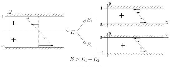
Figure 7: An example showing the non-additivity of energy within the Euler equations for a shear flow.

Coulomb systems constitute another relevant example of long-range interactions, which are of type (18):

$$U(\vec{r}_{1},\ldots,\vec{r}_{N})=\frac{1}{4\pi\varepsilon_{0}}\sum_{1\leq i<j\leq N}e_{i}e_{j}V(|\vec{r_{i}}-\vec{r_{j}}|),$$ (37)

where $\varepsilon_{0}$ is the vacuum permittivity, and $e_{i}$ is the charge located at position $\vec{r_{i}}$. For such systems, it may be shown that the excess charge is expelled to the boundary of a domain, and that the bulk is neutral. A typical configuration has a distribution of charges of equal sign surrounded by a “cloud” of particles of opposite charge, which “screens” the interactions at long range. The effective two-body potential is therefore given by

$$V_{\rm eff}\propto\frac{\exp(-r/\lambda_{D})}{r},$$ (38)

where $\lambda_{D}\equiv(\varepsilon_{0}/(2ne^{2}\beta))^{1/2}$ is the so-called Debye length, and $n$ is the particle density. On account of the screening, Coulomb systems are effectively short-range.

A plasma of electrons can be confined by a crossed electric field $\mathbf{E}$ and a magnetic field $\mathbf{B}$ [13]. As shown in Fig. 8, the electrons are contained axially by negative voltages and radially by a uniform axial magnetic field $B_{z}$. Under typical experimental conditions of density and temperature, electrons are collisionless; They bounce axially very rapidly and drift across the magnetic field with velocity

$$\mathbf{v}=\frac{-\nabla\phi\times\hat{z}}{B_{z}}.$$ (39)

As is the case of an effectively incompressible fluid, the electron density $n(x,y)$ obeys the evolution equations

$$\frac{\partial n}{\partial t}+\mathbf{v}\cdot\nabla n=0,$$ (40)

$$\Delta\phi=\frac{en}{\varepsilon_{0}},$$ (41)

where $-e$ is electron charge. These equations are isomorphic to the two-dimensional Euler equations with vorticity $\omega=en/\varepsilon_{0}$ and stream function $\psi=\phi/B_{z}$. The electron plasma may be regarded as the best experimental realization of two-dimensional incompressible, inviscid fluid.

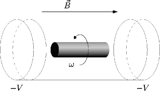
Figure 8: Plasma of electrons confined by crossed electric and magnetic fields.

Dipolar interaction is marginally long-range [14]: $\alpha=3$ in $d=3$. The interaction energy of two dipoles is

$$E_{ij}=\frac{\mu_{0}}{4\pi}\left[\frac{\vec{\mu}_{i}\cdot\vec{\mu}_{j}}{|\vec{r}_{ij}|^{3}}-\frac{3(\vec{\mu}_{i}\cdot\vec{r}_{ij})(\vec{\mu}_{j}\cdot\vec{r}_{ij})}{|\vec{r}_{ij}|^{5}}\right],$$ (42)

where $\mu_{0}$ is vacuum permeability, and $\vec{\mu}_{i}$ is the dipolar moment at position site $\vec{r}_{i}$. Because of the anisotropy of the interaction, dipolar systems are strongly frustrated: several configurations have the same energy. For ferromagnetic samples of ellipsoidal shape, one has the total energy

$$E_{\rm Dipolar}=\frac{1}{2}\sum_{i,j}E_{ij}=E_{0}V+\frac{1}{2}\mu_{0}\frac{(\sum_{i}\vec{\mu}_{i})^{2}}{V}D,$$ (43)

where $E_{0}$ is a local-energy term that depends on the crystal structure, and $D$ is the so-called shape-dependent demagnetizing factor: $D=1/3$ for spherical samples, $D=0$ for needle shape samples, $D=1$ for disk shaped samples. The free energy of a dipolar magnetic system is shape-independent, which implies that the macroscopic state cannot be ferromagnetic. However, ferromagnetism can exist in mesoscopic samples, paving the way to the possible experimental detection of long-range effects.

An experimental apparatus where long-range forces are at play is the free-electron laser [15]. In the linear free-electron laser, a relativistic electron beam propagates through a spatially periodic magnetic field, interacting with the co-propagating electromagnetic wave, see Fig. 9. Lasing occurs when the electrons bunch in a subluminar beat wave. After scaling away the time dependence of the phenomenon, and on introducing appropriate variables, e.g., the length $z$ along the lasing direction, it is possible to capture the essence of the asymptotic state by studying the following equations of motion first introduced by Colson and Bonifacio:

$$\frac{{\rm d}\theta_{j}}{{\rm d}z} = p_{j},$$ (44)

$$\frac{{\rm d}p_{j}}{{\rm d}z} = -\mathbf{A}e^{i\theta_{j}}-\mathbf{A}^{\ast}e^{-i\theta_{j}},$$ (45)

$$\frac{{\rm d}\mathbf{A}}{{\rm d}z} = i\delta\mathbf{A}+\frac{1}{N}\sum_{j}e^{-i\theta_{j}}.$$ (46)

The above equations derive from the Hamiltonian

$$H_{\rm FEL}=\sum_{j=1}^{N}\frac{p_{j}^{2}}{2}-N\delta A^{2}+2A\sum_{j=1}^{N}\sin(\theta_{j}-\varphi).$$ (47)

The $p_{i}$’s are related to the energies relative to the center of mass of the $N$-electron system, and the conjugated variables $\theta_{i}$ characterize their positions with respect to the co-propagating wave. The complex electromagnetic field variable, $\mathbf{A}=A\,e^{i\varphi}$, defines the amplitude and the phase of the dominating mode ($\mathbf{A}$ and $\mathbf{A}^{\star}$ are canonically conjugate variables). The parameter $\delta$ measures the average deviation from the resonance condition.

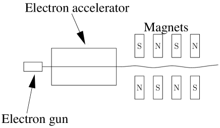
Figure 9: Sketch of a linear free-electron laser.

3 Dynamical evolution of LRI systems: The general scenario

In this Section, we discuss the general scenario of dynamical evolution of isolated LRI systems. To this end, let us consider an interacting system of $N$ identical particles of mass $m$, which we take for simplicity of discussion to be embedded in one-dimensional ($1d$) space (the discussions straightforwardly generalize to higher dimensions). The Hamiltonian of the system is given by

$$H=\sum_{i=1}^{N}\frac{p_{i}^{2}}{2m}+\sum\limits_{1\leq i<j\leq N}^{N}V(|q_{i}-q_{j}|),$$ (48)

where $q_{i}\in{\cal D}$ are the canonical coordinates of the particles, and $p_{i}\in\mathbb{R}$ are the corresponding conjugated momenta. Here, $V(|q_{i}-q_{j}|)$ is the two-body interaction potential between particles $i$ and $j$. We consider ${\cal D}$ to be finite and with periodic boundary conditions, and set $m=1$ in the following without loss of generality.

A microstate of the system is specified by giving the coordinates and the momenta of all the particles, and defines a representative point ${\bf z}$, with $z_{i}\equiv(p_{i},q_{i});~{}i=1,2,\ldots,N$, in the $2N$-dimensional phase space $\Gamma$ of the system. A distribution of representative points in the phase space, corresponding to different microstates of the system consistent with a given macrostate, is characterized by the $N$-particle phase space density $\rho(z_{1},z_{2},\ldots,z_{N},t)$, defined such that $\rho(z_{1},z_{2},\ldots,z_{N},t){\rm d}z_{1}{\rm d}z_{2}\ldots{\rm d}z_{N}$, with ${\rm d}z_{i}\equiv{\rm d}p_{i}{\rm d}q_{i}$, gives the number of representative points contained at time $t$ in an infinitesimal volume element $\prod_{i=1}^{N}{\rm d}z_{i}$ around the point ${\bf z}$. In view of the particles constituting the system being identical, we consider the $N$-particle density to be symmetric in $z_{1},z_{2},\ldots,z_{N}$. As the microstates evolve in time following the Hamilton equations

$$\dot{p}_{i}=-\frac{\partial H}{\partial q_{i}},~{}~{}\dot{q}_{i}=\frac{\partial H}{\partial p_{i}},$$ (49)

with a dot denoting derivative with respect to time, the phase space density evolves in time following the Liouville’s theorem ${\rm d}\rho/{\rm d}t=0$; Combined with the Hamilton equations, this implies

$$\frac{\partial\rho}{\partial t}+\sum\limits_{i=1}^{N}\Big{[}p_{i}\frac{\partial\rho}{\partial q_{i}}-\frac{\partial\rho}{\partial p_{i}}\frac{\partial}{\partial q_{i}}\sum\limits_{j=1,j\neq i}^{N}V(|q_{i}-q_{j}|)\Big{]}=0.$$ (50)

Since Liouville’s theorem implies that $\int\prod_{i=1}^{N}{\rm d}z_{i}~{}\rho(z_{1},z_{2},\ldots,z_{N},t)$ is a constant in time, we may choose this constant to be unity, implying the normalization $\int\prod_{i=1}^{N}{\rm d}z_{i}~{}\rho(z_{1},z_{2},\ldots,z_{N},t)=1$.

Using the $N$-particle density $\rho(z_{1},z_{2},\ldots,z_{N},t)$, one may define a single-particle density as

$$f_{1}(z_{1},t)\equiv\int\prod_{i=2}^{N}{\rm d}z_{i}~{}\rho(z_{1},z_{2},\ldots,z_{N},t).$$ (51)

The physical interpretation of $f_{1}$ is as follows: In contrast to the $2N$-dimensional $\Gamma$ space, one may construct a $2$-dimensional single-particle phase space $\mu$, with axes $(p,q)$, in which a microstate of the system is represented by $N$ representative points $(z_{1},z_{2},\ldots,z_{N})$. A distribution of points in the $\Gamma$ space may be mapped to a distribution in the $\mu$ space. The latter is characterized by the single-particle phase space density $f_{1}(p,q,t)$, defined such that $f_{1}(p,q,t){\rm d}p{\rm d}q$ gives the number of representative points contained at time $t$ in an infinitesimal volume element ${\rm d}p{\rm d}q$ centered at $(p,q)$. As it will turn out, it will often be convenient and meaningful to discuss the evolution of an LRI system in the $\mu$ space rather than in the higher dimensional $\Gamma$ space. Using $\rho(z_{1},z_{2},\ldots,z_{N},t)$, one may in general define the $s$-particle density

$$f_{s}(z_{1},z_{2},\ldots,z_{s},t)=\frac{N!}{(N-s)!}\int\prod_{i=s+1}^{N}{\rm d}z_{i}~{}\rho(z_{1},z_{2},\ldots,z_{N},t);~{}~{}s=1,2,\ldots,N.$$ (52)

In view of the normalization of $\rho(z_{1},z_{2},\ldots,z_{N},t)$, one has $\int{\rm d}z~{}f_{1}(z,t)=N$, and in general, $\int\prod_{i=1}^{s}{\rm d}z_{i}~{}f_{s}(z_{1},z_{2},\ldots,z_{s},t)=N!/(N-s)!$.

Using Eq. (50), one may derive the time evolution of $f_{s}$ to find that a determination of its evolution requires knowing the higher density $f_{s+1}$. It then follows that the time evolution of the full set $(f_{1},f_{2},f_{3},\ldots,f_{N})$ forms a coupled chain of equations, which goes by the name of the Bogoliubov-Born-Green-Kirkwood-Yvon (BBGKY) hierarchy. The first equation of the hierarchy reads

$$\Big{[}\frac{\partial}{\partial t}+p_{1}\frac{\partial}{\partial q_{1}}\Big{]}f_{1}(z_{1},t)=\int{\rm d}z_{2}~{}\frac{\partial}{\partial q_{1}}V(|q_{1}-q_{2}|)\frac{\partial}{\partial p_{1}}f_{2}(z_{1},z_{2},t).$$ (53)

Now, we may express the two-particle density quite generally as

$$f_{2}(z_{1},z_{2},t)=f_{1}(z_{1},t)f_{1}(z_{2},t)+g_{2}(z_{1},z_{2},t),$$ (54)

where $g_{2}$ describes the two-particle correlation. Integrating both sides with respect to $(z_{1},z_{2})$, it then follows that $g_{2}\sim N$. For an LRI system, let us now invoke Kac’s trick, $J\to J/N$, implying $V\to V/N$. Then, using Eq. (53), and noting that $f_{1}\sim N$, one obtains to leading order in $1/N$ the evolution equation [16]

$$\Big{[}\frac{\partial}{\partial t}+p_{1}\frac{\partial}{\partial q_{1}}\Big{]}f_{1}(z_{1},t)=\frac{\partial\Phi}{\partial q_{1}}\frac{\partial}{\partial p_{1}}f_{1}(z_{1},t),$$ (55)

where $\Phi[f_{1}](q_{1},t)=\int{\rm d}z_{2}~{}V(|q_{1}-q_{2}|)f_{1}(z_{2},t)$ is the mean-field potential. Equation (55) that describes the time evolution of the single-particle phase space density is called the Vlasov equation.

In passing, we note that for a short-range system for which no Kac scaling needs to be invoked, Eq. (53) yields to leading order in $1/N$ the evolution equation

$$\Big{[}\frac{\partial}{\partial t}+p_{1}\frac{\partial}{\partial q_{1}}\Big{]}f_{1}(z_{1},t)=\int{\rm d}z_{2}~{}\frac{\partial}{\partial q_{1}}V(|q_{1}-q_{2}|)\frac{\partial}{\partial p_{1}}g_{2}(z_{1},z_{2},t).$$ (56)

The difference of the above equation from the Vlasov equation (55) is evident. To leading order in $1/N$, the time evolution for an LRI system is governed by the mean-field potential (besides the trivial “streaming term” on the left hand side of both Eqs. (55) and (56) that is present even when the particles are noninteracting), with the two-particle correlation $g_{2}$ providing the next higher-order correction. Instead, for a short-range system, it is the two-particle correlation that dictates the leading time-evolution of the phase space density.

Let us remark on some relevant features of the Vlasov equation (55). The equation is evidently time-reversal invariant. One may associate with the equation a Hamilton dynamics due to a single-particle (mean-field) Hamiltonian ${\cal H}[f_{1}](p,q,t)=p^{2}/2+\Phi[f_{1}](q,t)$. Note that the presence of the mean-field potential makes this Hamiltonian a functional of the single-particle density $f_{1}$. One may then rewrite the Vlasov equation in terms of a Poisson bracket:

$$\frac{\partial f_{1}}{\partial t}+\{f_{1},{\cal H}\}=0,$$ (57)

which implies that Vlasov-stationary solutions ($\partial f_{1}/\partial t=0$) are given by arbitrary normalizable functions of the single-particle Hamiltonian, as $f_{1}(p,q)=F({\cal H})$. Another class of stationary solutions involves those that are homogeneous in the position coordinate ($\partial f_{1}/\partial q=0$), that is, $f_{1}(p,q)\propto h(p)$, where $h(p)$ is a normalizable function of the momentum. Given the extent of arbitrariness allowed in choosing the functions $F$ and $h$, one may conclude that the Vlasov equation admits an infinite number of stationary solutions. These stationary solutions define the so-called “Vlasov equilibrium” state of the system. Furthermore, the equation admits an infinite number of conserved quantities, the so-called Casimirs $C[f_{1}]=\int{\rm d}p{\rm d}q~{}c(f_{1}(q,p))$, with $c$ an arbitrary function of its argument. In particular, the single-particle entropy $S[f_{1}]\equiv-\int{\rm d}p{\rm d}q~{}f_{1}\ln f_{1}$ is a conserved quantity, and is thus constant in time.

The leading correction to the Vlasov equation is given by

$$\Big{[}\frac{\partial}{\partial t}+p_{1}\frac{\partial}{\partial q_{1}}\Big{]}f_{1}(z_{1},t)-\frac{\partial\Phi}{\partial q_{1}}\frac{\partial}{\partial p_{1}}f_{1}(z_{1},t)=\int{\rm d}z_{2}~{}\frac{\partial}{\partial q_{1}}V(|q_{1}-q_{2}|)\frac{\partial}{\partial p_{1}}g_{2}(z_{1},z_{2},t).$$ (58)

Noting that $f_{1}\sim N$ and $g_{2}\sim N$, the above equation implies time evolution of Vlasov-stationary solutions on timescales of $O(N)$.

The second equation of the BBGKY hierarchy is

$$\Big{[}\frac{\partial}{\partial t}+p_{1}\frac{\partial}{\partial q_{1}}+p_{2}\frac{\partial}{\partial q_{2}}-\frac{\partial}{\partial q_{1}}V(|q_{1}-q_{2}|)\frac{\partial}{\partial p_{1}}-\frac{\partial}{\partial q_{2}}V(|q_{1}-q_{2}|)\frac{\partial}{\partial p_{2}}\Big{]}f_{2}(z_{1},z_{2},t)$$

$$=\int{\rm d}z_{3}~{}\Big{[}\frac{\partial}{\partial q_{1}}V(|q_{1}-q_{3}|)\frac{\partial}{\partial p_{1}}+\frac{\partial}{\partial q_{2}}V(|q_{2}-q_{3}|)\frac{\partial}{\partial p_{2}}\Big{]}f_{3}(z_{1},z_{2},z_{3},t).$$ (59)

Similar to the decomposition (54), one has for the three-point correlation

$$f_{3}(z_{1},z_{2},z_{3},t) = f_{1}(z_{1},t)f_{1}(z_{2},t)f_{1}(z_{3},t)+f_{1}(z_{1},t)g_{2}(z_{2},z_{3},t)$$ (60)

$$+f_{1}(z_{2},t)g_{2}(z_{1},z_{3},t)+f_{1}(z_{3},t)g_{2}(z_{1},z_{2},t)+h(z_{1},z_{2},z_{3},t),$$

where, arguing as for Eq. (54), one concludes that $h\sim N$. Using Eqs. (54) and (60) in Eq. (59), and using the Kac’s scaling $V\to V/N$, one obtains to leading order in $1/N$ the result

$$\frac{\partial g_{2}(z_{1},z_{2},t)}{\partial t} = \Big{(}\frac{\partial}{\partial q_{1}}V(|q_{1}-q_{2}|)\frac{\partial}{\partial p_{1}}g_{2}(z_{1},z_{2},t)-p_{1}\frac{\partial}{\partial q_{1}}g_{2}(z_{1},z_{2},t)$$ (61)

$$+f_{1}(z_{1},t)\frac{\partial}{\partial q_{2}}\Big{[}\int{\rm d}z_{3}~{}V(|q_{2}-q_{3}|)f_{1}(z_{3},t)\Big{]}\frac{\partial}{\partial p_{2}}f_{1}(z_{2},t)$$

$$+\frac{\partial}{\partial q_{1}}\Big{[}\int{\rm d}z_{3}~{}V(|q_{1}-q_{3}|)f_{1}(z_{3},t)\Big{]}\frac{\partial}{\partial p_{1}}g_{2}(z_{1},z_{2},t)$$

$$+\frac{\partial}{\partial p_{1}}f_{1}(z_{1},t)\frac{\partial}{\partial q_{1}}\int{\rm d}z_{3}~{}V(|q_{1}-q_{3}|)g_{2}(z_{2},z_{3},t)\Big{)}+\{1\leftrightarrow 2\}$$

$$\equiv A[f_{1},g_{2}],$$

where $\{1\leftrightarrow 2\}$ implies including terms obtained from the bracketed ones by exchanging the subscripts $1$ and $2$, and $A$ is a functional of $f_{1}$ and $g_{2}$.

On the basis of the above discussion, let us summarize the general scenario of relaxation in LRI systems, see Fig. 10. In a first stage of violent relaxation, the system goes from a generic initial condition towards a Vlasov-stable stationary state on a fast timescale independent of the number of particles. In a second stage of collisional relaxation, finite-$N$ effects drive the system through a sequence of Vlasov-stable states towards the Boltzmann-Gibbs equilibrium state on a timescale that is strongly dependent on $N$. Often, the latter scale is a power law $\sim N^{\gamma};~{}~{}\gamma>0$; A typical example is the Chandrasekhar relaxation timescale for stellar systems, which is proportional to $N/\ln N$. The Vlasov-stable stationary states have been named the quasistationary states (QSSs), since such states emerge as the true stationary states on taking the $N\to\infty$ limit first, followed by the limit $t\to\infty$. An example of a spiral galaxy “stuck” in a QSS is shown in Fig. 10.

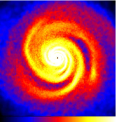
Figure 10: (Left panel) Schematic description of the typical dynamical evolution of LRI systems. Here, $\tau_{v}$ and $\tau_{c}$ are the violent relaxation and the collisional relaxation timescale, respectively. (Right panel) A spiral galaxy.

4 A model with discrete degrees of freedom: The Kardar-Nagel model

A solvable model of LRI systems involving discrete degrees of freedom, which shows such features stemming from long-range interactions as ensemble inequivalence and slow relaxation, is the so-called Kardar-Nagel model [17]. The Hamiltonian reads

$$H_{\rm KN}=-\frac{K}{2}{\sum_{i=1}^{N}}\left(S_{i}S_{i+1}-1\right)-\frac{J}{2N}\left({\sum_{i=1}^{N}}S_{i}\right)^{2},$$ (62)

and involves spins $S_{i}=\pm 1$ occupying the sites of a one-dimensional lattice. The spins are coupled with nearest-neighbors with strength $K$, and with an additional Curie-Weiss ferromagnetic ($J>0$) interaction. In the following, we set $J$ to unity without loss of generality.

The solution in the canonical ensemble: The canonical partition function is

$$Z(\beta,N)=\sum_{\{S_{1},\ldots,S_{N}\}}e^{-\beta H}=\sum_{\{S_{1},\ldots,S_{N}\}}\exp\left[{\displaystyle\frac{\beta}{2N}\left(\sum_{i=1}^{N}S_{i}\right)^{2}+\frac{\beta K}{2}\sum_{i=1}^{N}\left(S_{i}S_{i+1}-1\right)}\right].$$

(63)

Using the Hubbard-Stratonovich transformation, the partition function may be rewritten as

$$Z(\beta,N)=\sqrt{\frac{\beta N}{2\pi}}\int_{-\infty}^{\infty}{\rm d}x~{}e^{\displaystyle-\frac{\beta N}{2}x^{2}}\,\sum_{\{S_{1},\ldots,S_{N}\}}\Biggl{[}e^{\displaystyle\beta x\sum_{i=1}^{N}S_{i}+\frac{\beta K}{2}\sum_{i=1}^{N}\left(S_{i}S_{i+1}-1\right)}\Biggr{]}$$

$$=\sqrt{\frac{\beta N}{2\pi}}\int_{-\infty}^{\infty}{\rm d}x~{}e^{\displaystyle-N\beta\widetilde{f}\left(\beta,x\right)}.$$ (64)

The free energy may be written as

$$\widetilde{f}(\beta,x)=\frac{1}{2}x^{2}+f_{0}(\beta,x),$$ (65)

where $f_{0}(\beta,x)$ is the free energy of the nearest-neighbor Ising model in an external field of strength $x$, which may be easily derived using the transfer matrix: $f_{0}(\beta,x)=-\ln(\lambda_{+}^{N}+\lambda_{-}^{N})/(\beta N)$, where the two eigenvalues of the transfer matrix are

$$\lambda_{\pm}=e^{\beta K/2}\cosh(\beta x)\pm\sqrt{e^{\beta K}\sinh^{2}(\beta x)+e^{-\beta K}}.$$ (66)

As $\lambda_{+}>\lambda_{-}$ for all values of $x$, only the larger eigenvalue $\lambda_{+}$ is relevant in the limit $N\rightarrow\infty$. One thus finally gets

$$\widetilde{\phi}(\beta,x)\equiv\beta\widetilde{f}(\beta,x)=\frac{\beta}{2}x^{2}-\ln\left[e^{\beta K/2}\cosh(\beta x)+\sqrt{e^{\beta K}\sinh^{2}(\beta x)+e^{-\beta K}}\right].$$ (67)

In the large $N$-limit, the application of the saddle point method to Eq. (64) implies taking the value of $x$ that minimizes $\widetilde{\phi}(\beta,x)$ in formula (67), thereby yielding the free energy. From the knowledge of the free energy, one gets either a continuous or a first-order phase transition depending on the value of the coupling constant $K$. An expansion of $\widetilde{f}(\beta,x)$ in powers of $x$ yields

$$\widetilde{f}(\beta,x)=-\ln 2\cosh\frac{\beta K}{2}+\frac{\beta}{2}x^{2}\left(1-\beta e^{\beta K}\right)+\frac{\beta^{4}}{24}e^{\beta K}\left(3e^{2\beta K}-1\right)x^{4}+{\cal O}(x^{6}).$$ (68)

The critical point of the continuous transition is obtained for each $K$ by computing the value $\beta_{c}$ at which the quadratic term of the expansion (68) vanishes, provided the coefficient of the fourth-order term is positive, thus obtaining $\beta_{c}=\exp{(-\beta_{c}K)}$. When also the fourth order coefficient vanishes, i.e., for $3\exp(2\beta K)=1$, one gets the canonical tricritical point (CTP) $K_{\rm CTP}=-\ln 3/(2\sqrt{3})\simeq-0.317$. The first-order line is obtained numerically by requiring that $f(\beta,0)=f(\beta,x^{*})$, where $x^{*}$ is the further local minimum of $f$.

The solution in the microcanonical ensemble: The magnetization $M\equiv\sum_{i=1}^{N}S_{i}$ may be expressed as $M=N_{+}-N_{-}$, by introducing the number of up-spins, $N_{+}$, and the number of down-spins, $N_{-}$. The first term of the Hamiltonian (62) may be expressed as $-M^{2}/(2N)$. As two identical neighboring spins would not contribute to the second term of the Hamiltonian, while two different ones would give a contribution equal to $K$, the total contribution of the second term is $KU$, where $U$ is the number of “kinks” in the chain, i.e., the number of links between two neighboring spins of opposite signs.

For a chain of $N$ spins, the number of microstates corresponding to an energy $E$ may be written as $\left(\begin{array}[]{ll}N_{+}\\ {\displaystyle U}/{\displaystyle 2}\end{array}\right)\left(\begin{array}[]{ll}N_{-}\\ {\displaystyle U}/{\displaystyle 2}\end{array}\right)$. The formula is derived by taking into account that one has to distribute $N_{+}$ spins among $U/2$ groups and $N_{-}$ among the remaining $U/2$; Each of these distributions gives a binomial term, and, since they are independent, the total number of states is the product of the two binomials. The expression is only approximate, because the model (62) is defined on a ring, but nevertheless, the corrections are of order $N$, and hence, do not contribute to the entropy. Introducing $m=M/N$, $u=U/N$ and $\varepsilon=E/N=-m^{2}/2+Ku$, one thus gets the entropy as

$$\widetilde{s}(\varepsilon,m)=\frac{1}{N}\,\ln\Omega=\frac{1}{2}(1+m)\ln(1+m)+\frac{1}{2}(1-m)\ln(1-m)-u\ln u$$

$$-\frac{1}{2}(1+m-u)\ln(1+m-u)-\frac{1}{2}(1-m-u)\ln(1-m-u).$$ (69)

In the large $N$-limit, maximizing the entropy $\widetilde{s}(\varepsilon,m)$ with respect to the magnetization $m$ leads to the final expression for the entropy: $s(\varepsilon)=\widetilde{s}(\varepsilon,m^{*})$, where $m^{*}$ is the equilibrium value. An expansion of $\widetilde{s}(\varepsilon,m)$ in powers of $m$ yields

$$\widetilde{s}(\varepsilon,m)=s_{0}(\varepsilon)+A_{\rm mc}m^{2}+B_{\rm mc}m^{4}+{\cal O}(m^{4}),$$ (70)

with the paramagnetic zero-magnetization entropy given by

$$s_{0}(\varepsilon)=-\frac{\varepsilon}{K}\ln\frac{\varepsilon}{K}-\left(1-\frac{\varepsilon}{K}\right)\ln\left(1-\frac{\varepsilon}{K}\right),$$ (71)

and the expansion coefficients

$$A_{\rm mc} = \frac{1}{2}\left[\frac{1}{K}\ln\frac{K-\varepsilon}{\varepsilon}-\frac{\varepsilon}{K-\varepsilon}\right],$$ (72)

$$B_{\rm mc} = \frac{\varepsilon^{3}}{12(\varepsilon-K)^{3}}-\frac{K^{2}+K}{4(\varepsilon-K)^{2}}+\frac{1}{8K\varepsilon}.$$ (73)

Using these expressions, it is straightforward to find the continuous transition line by requiring that $A_{\rm mc}=0$ ($B_{\rm mc}<0$), finding $\beta_{c}=\exp(-\beta_{c}K)$, which is the same equation as found in the canonical ensemble. Thus, as far as the continuous phase transitions are concerned, the two ensembles are equivalent. The tricritical point is obtained by the condition $A_{\rm mc}=B_{\rm mc}=0$, giving $K_{\rm MTP}\simeq-0.359$ and $\beta_{\rm MTP}\simeq 2.21$, which is different from $K_{\rm CTP}\simeq-0.317$ and $\beta_{\rm CTP}=\sqrt{3}$. The microcanonical first-order phase transition line is obtained numerically by equating the entropies of the ferromagnetic and paramagnetic phases. At a given transition energy, there are two temperatures, thus leading to a temperature jump. The model also exhibits a region of negative specific heat when the phase transition is first-order in the canonical ensemble. The phase diagram of the model in the $(K,T)$ plane is shown in Fig. 11. One may observe the region of inequivalence between the microcanonical and the canonical ensemble for $K<0$.

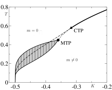
Figure 11: Phase diagram of the Kardar-Nagel model, Eq. (62). In the canonical ensemble, the large-$K$ transition is continuous (bold solid line) down to the tricritical point CTP, where it becomes first-order (dashed line). In the microcanonical ensemble, the continuous transition coincides with the canonical one at large $K$ (bold line); It persists at lower $K$ (dotted line) down to the tricritical point MTP, where it becomes first-order, with a branching of the transition line (solid lines). The region between these two lines (shaded area) is not accessible in the microcanonical ensemble.

The Kardar-Nagel model shows broken ergodicity, because presence of long-range interactions and the implied non-additivity make the region of macroscopic accessible states non-convex. Consider positive-magnetizations states, $N_{+}>N_{-}$, so that $0<U<2N_{-}=N-M$, which in turn implies in the limit $N\to\infty$ that

$$0\leq u=\frac{\varepsilon}{K}+\frac{J}{2K}m^{2}\leq 1-m.$$ (74)

As a consequence, the allowed magnetization-energy states are those within the shaded area in Fig. 12. From the figure, it is evident that there are energies (for instance, $\varepsilon=-0.35$) for which the magnetization has three allowed values within three different intervals: one around $m=0$, and two around opposite values of $m$. Any continuous energy-conserving dynamics initiated in one of these intervals would now allow for a transition to states belonging to another interval, so that ergodicity on the energy surface is broken. An example of breaking of ergodicity is shown in Fig. 13. In the upper panel, the dynamics is run at an energy, $\varepsilon=-0.318$, for which the energy surface is connected and the system is ergodic. Nevertheless, the magnetization jumps among the three maxima of the entropy (shown in the inset). In the lower panel, the energy is $\varepsilon=-0.325$, and the accessible values of the magnetization lie in three disjoint intervals. Therefore, if the initial magnetization lies around zero, its value remains around zero forever in time, as shown in one of the time series. In the other, the magnetization remains at a positive value. No transition among the zero and the non-zero magnetization state is possible. Entropy, shown in the insets, has gaps, corresponding to regions where the density of states is zero.

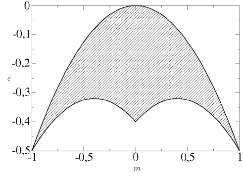
Figure 12: Allowed magnetization $m$ - energy $\varepsilon$ states for the Kardar-Nagel model, Eq. (62), with $K=-0.4$ and $J=1$.

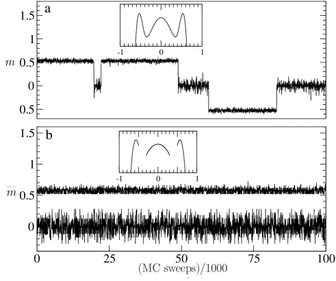
Figure 13: Microcanonical Monte Carlo simulation of the Kardar-Nagel model, Eq. 62, with $K=-0.4$ and $J=1$ and at different energies, showing ergodicity breaking (Lower panel).

We now briefly discuss how we may simulate the dynamics of the model (62) within the microcanonical ensemble with conserved energy $E$ by Monte Carlo simulations, using the so-called Creutz algorithm. In this algorithm, one probes the microstates of the system with energy $\leq E$, by adding an auxiliary variable called the “demon”, such that

$$E_{S}+E_{D}=E,$$ (75)

with $E_{S}$ being the energy of the system, and $E_{D}>0$ being that of the demon. The simulation begins with $E_{S}=E$, $E_{D}=0$, and attempt a spin flip. The move is accepted if the energy decreases, and the excess energy resulting from the flip is given to the demon:

$$E_{S}\to E_{S}-\Delta E,~{}E_{D}\to E_{D}+\Delta E,~{}\Delta E>0.$$ (76)

If instead the energy increases due to the spin flip, the energy needed to flip the spin is taken from the demon:

$$E_{S}\to E_{S}+\Delta E,~{}E_{D}\to E_{D}-\Delta E,~{}\Delta E>0,$$ (77)

provided the demon has the needed energy; otherwise, the move is rejected, but one keeps the configuration in the computation of averages. It can be proven that this dynamics respects detailed balance, and that the microcanonical measure (all configurations have equal weights on the energy surface) is stationary. One can also prove that the probability distribution of the demon energy is exponential:

$$p(E_{D})\propto\exp(-\beta E_{D}),$$ (78)

and uses this property to determine the microcanonical inverse temperature $\beta$.

5 A model with continuous degrees of freedom: The Hamiltonian mean-field (HMF) model

The Hamiltonian mean-field (HMF) model is a model involving continuous degrees of freedom and evolving under Hamilton dynamics. The model has emerged over the years as a prototypical model to study and elucidate the many peculiar features resulting from long-range interactions [18]. The HMF model also mimics physical systems like gravitational sheet models and free-electron lasers. In order to derive the model, we start with the Hamiltonian (48), take the mass to be unity without loss of generality, and consider the potential to be $V(q)\propto Jq^{-\alpha};~{}0\leq\alpha\leq 1$, for large $q$, so that in accordance with the Kac prescription, we scale the coupling constant $J$ by $N$ to make the total energy extensive in $N$. Next, we assume periodic coordinates so that boundary effects may be neglected. From now on, we denote the coordinates by periodic variables $\theta_{i}$’s, with $\theta_{i}\in[-\pi,\pi]$, so that $V(\theta)=V(\theta+2\pi)$. The interparticle potential $V(\theta)$, which by definition is an even function to satisfy Newton’s third law of motion, may be expanded in a cosine Fourier series: $V(\theta)=\widetilde{v}_{0}/2+\sum_{k=1}^{\infty}\widetilde{v}_{k}\cos(k\theta)$; retaining only the first Fourier term, one obtains the HMF model. The corresponding Hamiltonian is given by

$$H=\sum_{i=1}^{N}\frac{p_{i}^{2}}{2}+\frac{1}{N}\sum_{1\leq i<j\leq N}^{N}\left[1-\cos\left(\theta_{i}-\theta_{j}\right)\right],$$ (79)

which effectively describes a system of globally interacting point particles moving on a circle, with $\theta_{i}$ the angular coordinate of the $i$-th particle on the circle, and $p_{i}$ the corresponding conjugated momentum. In the Hamiltonian (79), we have without loss of generality further assumed the interparticle interaction to be attractive, by setting the coupling constant $J$ to unity. The HMF model may also be seen as a system of mean-field $XY$ spins, only that here, the Poisson bracket of the spin components is identically zero. The Hamiltonian (79) is invariant under the O$(2)$ symmetry group. As we show below, in thermal equilibrium and for energy densities smaller than $\varepsilon_{c}\equiv 3/4$, the symmetry is spontaneously broken to result in a clustered state, thereby leading to a continuous phase transition at $\varepsilon_{c}$. The order parameter of clustering is the magnetization $m\equiv\sqrt{m_{x}^{2}+m_{y}^{2}}$, with

$$(m_{x},m_{y})\equiv\frac{1}{N}\left(\sum_{i=1}^{N}\cos\theta_{i},\sum_{i=1}^{N}\sin\theta_{i}\right).$$ (80)

We now derive the equilibrium solution of the model. After the trivial Gaussian integration over the momenta, the canonical partition function is given by

$$Z(\beta,N)=\exp\left(-\frac{N\beta}{2}\right)\left(\frac{2\pi}{\beta}\right)^{N/2}$$

$$\times\int\mbox{d}\theta_{1}\dots\mbox{d}\theta_{N}~{}\exp\left\{\frac{\beta}{2N}\left[\left(\sum_{i=1}^{N}\cos\theta_{i}\right)^{2}+\left(\sum_{i=1}^{N}\sin\theta_{i}\right)^{2}\right]\right\}.$$ (81)

Using the Hubbard-Stratonovich transformation, we get

$$Z(\beta,N)=\exp\left(-\frac{N\beta}{2}\right)\left(\frac{2\pi}{\beta}\right)^{N/2}$$

$$\times\frac{N\beta}{2\pi}\int\mbox{d}x_{1}\mbox{d}x_{2}~{}\exp\left\{N\left[-\frac{\beta(x_{1}^{2}+x_{2}^{2})}{2}+\ln I_{0}(\beta(x_{1}^{2}+x_{2}^{2})^{\frac{1}{2}})\right]\right\},$$ (82)

where $I_{0}(z)$ is the modified Bessel function of order $0$: $I_{0}(z)\equiv\int_{0}^{2\pi}\mbox{d}\theta~{}\exp\left(z_{1}\cos\theta+z_{2}\sin\theta\right)=\int_{0}^{2\pi}\mbox{d}\theta~{}\exp\left(z\cos\theta\right)$, with $z\equiv\left(z_{1}^{2}+z_{2}^{2}\right)^{1/2}$. Going to polar coordinates in the $(x_{1},x_{2})$ plane yields

$$Z(\beta,N)=\exp\left(-\frac{N\beta}{2}\right)\left(\frac{2\pi}{\beta}\right)^{N/2}N\beta\int_{0}^{\infty}\mbox{d}x~{}x\exp\left\{N\left[-\frac{\beta x^{2}}{2}+\ln I_{0}(\beta x)\right]\right\}.$$ (83)

In the thermodynamic limit $N\rightarrow\infty$, the integral in (83) can be computed by using the saddle point method that involves the extremization problem of finding the particular value of $x$ that extremizes the function $\left[-\frac{\beta x^{2}}{2}+\ln I_{0}(\beta x)\right]$, and thus involves solving the equation

$$x=\frac{I_{1}(\beta x)}{I_{0}(\beta x)},$$ (84)

where $I_{1}(z)=I_{0}^{\prime}(z)$ is the modified Bessel function of order $1$. In terms of the solution of this extremization problem, one finally obtains the rescaled free energy per particle as

$$\phi(\beta)\equiv\beta f(\beta)=\frac{\beta}{2}-\frac{1}{2}\ln 2\pi+\frac{1}{2}\ln\beta+\inf_{x\geq 0}\left[\frac{\beta x^{2}}{2}-\ln I_{0}(\beta x)\right],$$ (85)

where note that one has to choose the particular solution of (84) that minimizes the free energy (85). For $\beta\leq 2$, the solution of Eq. (84) is given by $x=m^{*}=0$, while for $\beta\geq 2$, the solution monotonically increases with $\beta$, approaching $m^{*}=1$ for $\beta\rightarrow\infty$. The solution $m^{*}=0$ of (84), present for all values of $\beta$, may be discarded for $\beta>2$, since it does not minimize the free energy. One may show that the value $m^{*}$ realizing the extremum in Eq. (85) is equal to the spontaneous magnetization in equilibrium. Note from the foregoing discussions that the spontaneous magnetization is defined only up to its modulus, while there is a continuous degeneracy in its direction. We have thus shown that the HMF model displays a continuous phase transition at $\beta_{c}=2$ ($T_{c}=0.5$). The derivative of the rescaled free energy with respect to $\beta$ gives the energy per particle as

$$\varepsilon(\beta)=\frac{1}{2\beta}+\frac{1}{2}-\frac{1}{2}(m^{*}(\beta))^{2}.$$ (86)

As already evident from the Hamiltonian, the lower bound of $\varepsilon$ is $0$. At the critical temperature, the energy is $\varepsilon_{c}=3/4$. Since we have shown that the HMF model has a continuous phase transition in the canonical ensemble, we conclude that microcanonical and canonical ensembles are equivalent for this model.

For the system (79), one may easily write down the following Vlasov equation for the evolution of the single-particle phase space density $f(q,p,t)$ (cf. Eq. (55)):

$$\frac{\partial f}{\partial t}+p\frac{\partial f}{\partial\theta}-\frac{\partial\Phi}{\partial\theta}\frac{\partial f}{\partial p}=0,$$ (87)

where one has the mean-field potential

$$\Phi[f](\theta,t)=-\int_{0}^{2\pi}{\rm d}\theta^{\prime}\int_{-\infty}^{\infty}{\rm d}p~{}\cos(\theta-\theta^{\prime})f(\theta^{\prime},p,t).$$ (88)

For distributions that are homogeneous with respect to $\theta$, the mean-field potential evaluates to zero, implying that such distributions are stationary solutions of the Vlasov equation (87). Let us denote such homogeneous stationary solutions by $f_{0}(p)$. Since stationarity does not guarantee stability, one may study the stability of such homogeneous distributions with respect to small perturbations, by linearizing the Vlasov equation (87) about $f_{0}(p)$. One obtains the result that the homogeneous distribution $f_{0}(p)$ is stable if and only if the quantity

$$I\equiv 1+\frac{1}{2}\int_{-\infty}^{\infty}{\rm d}p~{}\frac{f_{0}^{\prime}(p)}{p}$$ (89)

is positive. Such a condition reveals that there can be an infinite number of Vlasov-stable stationary distributions. Let us briefly discuss some examples of $f_{0}(p)$.

• The first one is the Gaussian distribution: $f_{0}(p)\sim\exp({-\beta p^{2}/2})$, which is expected at equilibrium. With the threshold condition (89), one recovers the result due to statistical mechanics reviewed above that the critical inverse temperature is $\beta_{c}=2$, and its associated critical stability threshold is $\varepsilon^{\star}=\varepsilon_{c}=3/4$.

• The second example is the so-called water-bag distribution, which has often been used in the past to numerically demonstrate the out-of-equilibrium properties of the HMF model. Such a distribution comprises momentum uniformly distributed in a given interval $[-p_{0},p_{0}]$, where the parameter $p_{0}$ is related to the energy density as $p_{0}=\sqrt{6\varepsilon-3}$. In this case, one obtains the critical stability threshold as $\varepsilon^{\star}=7/12$: the state is linearly stable for energies larger than $\varepsilon^{\star}$, and is unstable below.

Let us emphasize that the above examples are Vlasov-stable stationary solutions that are possible among infinitely many others, and there is no reason to emphasize one over the other.

The existence of infinitely many Vlasov-stable stationary solutions of the HMF model implies that when starting initially from one such solution in the stable regime (e.g., the water-bag distribution at energy density $\varepsilon>\varepsilon^{\star}=7/12$), and evolving under the Hamilton equations derived from the Hamiltonian (79):

$$\frac{\mbox{d}\theta_{i}}{\mbox{d}t}=p_{i},~{}\frac{\mbox{d}p_{i}}{\mbox{d}t}=-m_{x}\sin\theta_{i}+m_{y}\cos\theta_{i},$$ (90)

the magnetization in an infinite system should remain zero at all times. For finite $N$, however, finite-$N$ effects drive the system away from the water-bag state, and through other stable stationary states. Such a slow quasi-stationary evolution across an infinite number of Vlasov-stable stationary states (note: stationary only in the limit $N\to\infty$) ends with the system in the Boltzmann-Gibbs (BG) equilibrium state, see Fig. 14. For the HMF model, it has been rigorously proven that Vlasov-stable homogeneous distributions do not evolve on timescales of order smaller or equal to $N$. Indeed, a scaling $\sim N^{\gamma};~{}\gamma>0$, for the timescale of relaxation towards the BG equilibrium state has been observed in simulations [19]. At long times, one has $m(t)\sim(1/\sqrt{N})e^{t/N^{\gamma}}$ for $t\gg N^{\gamma}$, where the prefactor accounts for finite-$N$ fluctuations. For $\varepsilon<\varepsilon^{*}$, linear instability results in a faster relaxation towards equilibrium as $m(t)\sim(1/\sqrt{N})e^{\gamma t}$ for $t\gg 1/\gamma$. Here, $\gamma^{2}=6\left(7/12-\varepsilon\right)$ is independent of $N$. Thus, there are no QSSs for energies below $\varepsilon^{*}$. Note that the slow relaxation to BG equilibrium depicted in Fig. 14 is consistent with the general scenario shown in Fig. 10. Recently, a theory using the so-called core-halo distributions has been proposed to quantitatively predict the properties of the QSSs [20]. A non-mean-field version of the HMF model, the so-called $\alpha$-HMF model, has been proposed and studied in Ref. [21] in the context of Lyapunov exponents, and in discussing the dominance of the mean-field mode in dictating the dynamics [22].

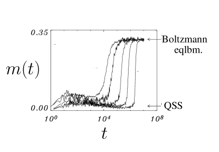
Figure 14: Time evolution of the modulus of the magnetization $m(t)$ for different particle numbers in the HMF model (79): $N=10^{3}$, $2\times 10^{3}$, $5\times 10^{3}$, $10^{4}$ and $2\times 10^{4}$ from left to right. The energy density is $\varepsilon=0.69$. The values of the magnetization indicated by the horizontal arrows refer respectively to the value expected in equilibrium (labelled BG) and the one corresponding to a homogeneous QSS.

5.1 An experimental realization of the HMF model: Atoms in optical cavities

Atoms interacting with a single-mode standing electromagnetic wave due to light trapped in a high-finesse optical cavity are subject to an inter-particle interaction that is long-ranged owing to multiple coherent scattering of photons by the atoms into the wave mode [23, 24, 25]. The set-up is shown in Fig. 15, which also shows optical pumping by a transverse laser of intensity $\Omega^{2}$ to counter the inevitable cavity losses quantified by the cavity linewidth $\kappa$. As regards the interaction with the electromagnetic field, each atom may be regarded as a two-level system, where the transition frequency between the two levels is $\omega_{0}$. Considering $N$ identical atoms of mass $m$ confined in one dimension along the cavity axis (taken to be the $x$-axis), and denoting the standing wave with wave number $k$ by $\cos(kx)$, the sum of the electric-field amplitudes coherently scattered by the atoms at time $t$ depends on their instantaneous positions $x_{1},\ldots,x_{N}$, and is proportional to the quantity $\Theta\equiv\sum_{j=1}^{N}\cos(kx_{j})/N$, so that the cavity electric field at time $t$ is $E(t)\propto\sqrt{N\overline{n}}\Theta$. Here, $\overline{n}$ is the maximum intra-cavity photon number per atom, given by $\overline{n}\equiv N\Omega^{2}\alpha^{2}/(\kappa^{2}+\Delta_{c}^{2})$, with $\alpha\equiv g/\Delta_{a}$ being the ratio between the cavity vacuum Rabi frequency and the detuning $\Delta_{a}\equiv\omega_{L}-\omega_{0}$ between the laser and the atomic transition frequency, and $\Delta_{c}\equiv\omega_{L}-\omega_{c}$ being the detuning between the laser and the cavity-mode frequency. The quantity $\Theta$ characterizes the amount of spatial ordering of atoms within the cavity mode, with $\Theta=0$ corresponding to atoms being uniformly distributed and the resulting vanishing of the cavity field, and $|\Theta|\neq 0$ implying spatial ordering. The wave number $k$ is related to the linear dimension $L$ of the cavity through $k=2\pi/\lambda$ and $L=q\lambda$, where $\lambda$ is the wavelength of the standing wave, and $q\in\mathbb{N}$.

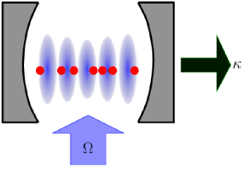
Figure 15: Atoms interacting with a single-mode standing electromagnetic wave in a cavity of linewidth $\kappa$, and being driven by a transverse laser with intensity $\Omega^{2}$.

The dynamics of the system is studied by analyzing the time evolution of the $N$-atom phase space distribution $f_{N}(x_{1},\ldots,x_{N},p_{1},\ldots,p_{N},t)$ at time $t$, with $p_{j}$’s denoting the momenta conjugate to the positions $x_{j}$. Treating the cavity field quantum mechanically, and regarding the atoms as classically polarizable particles with semi-classical center-of-mass dynamics, it may be shown that the distribution $f_{N}$ evolves in time according to the Fokker-Planck equation (FPE) [23, 24]

$$\partial_{t}f_{N}+\{f_{N},H\}=-\overline{n}\Gamma\sum_{i=1}^{N}\sin(kx_{i})\sum_{j=1}^{N}\partial_{p_{i}}\sin(kx_{j})\Big{(}p_{j}+\frac{m}{\beta}\partial_{p_{j}}\Big{)}f_{N}.$$ (91)

Here, $\Gamma\equiv 8\omega_{r}\kappa\Delta_{c}/(\Delta_{c}^{2}+\kappa^{2})$, $\hbar\beta\equiv-4\Delta_{c}/(\Delta_{c}^{2}+\kappa^{2})$, $\hbar$ is the reduced Planck constant, $\omega_{r}\equiv\hbar k^{2}/(2m)$ is the recoil frequency due to collision between an atom and a photon, while the Hamiltonian $H$ is given by

$$H\equiv\sum_{j=1}^{N}\frac{p_{j}^{2}}{2}-NJ\Theta^{2};~{}~{}J\equiv-\hbar\Delta_{c}\overline{n}.$$ (92)

The semi-classical limit is valid under the condition of $\kappa$ being larger than $\omega_{r}$, while Eq. (91) holds in a parameter regime in which processes describing a virtual scattering of cavity photons, which scale with the dynamical Stark shift of the cavity field $U=g\alpha$, are negligible. The Hamiltonian $H$ describes the conservative dynamical evolution of $f_{N}$ in the limit of vanishing cavity losses (or for times sufficiently small such that dissipative effects are negligible), and contains the photon-mediated long-ranged (mean-field) interaction between the atoms encoded in the second term on the right hand side (rhs) of Eq. (92). Note that the interaction is attractive (respectively, repulsive) when $\Delta_{c}$ is negative (respectively, positive). Cavity losses lead to damping and diffusion, which is described by the rhs of Eq. (91).

Let us now consider the case of effective attractive interactions between the atoms and the cavity field ($\Delta_{c}<0$), and study the dynamics of the system in the limit in which the effect of the dissipation may be neglected, that is, for sufficiently small times. In this limit, the dynamics of the $N$ atoms is conservative and governed by the Hamiltonian (92). The positions $x_{j}$ of the atoms enter the Hamiltonian only as $kx_{j}$, so that we may define the phase variables $\theta_{j}\equiv kx_{j}=2\pi x_{j}/\lambda$ for $j=1,\ldots,N$. Using $L=q\lambda$, and setting the origin of the $x$-axis in the center of the cavity, we have $x_{j}\in[-q\lambda/2,q\lambda/2]$, so that on using the periodicity of the cosine function, we can take the phase variables $\theta_{j}$ modulo $q$, yielding $\theta_{j}\in[-\pi,\pi]$. Then, by measuring lengths in units of the reciprocal wavenumber $k^{-1}=\lambda/(2\pi)$ of the cavity standing wave, masses in units of the mass of the atoms $m$, and energies in units of $\hbar\Delta_{c}$, the Hamiltonian may be rewritten in dimensionless form as

$$H=\sum_{j=1}^{N}\frac{(p_{\theta})_{j}^{2}}{2}-\overline{n}N\Theta^{2}\,,$$ (93)

where, in terms of the $\theta$ variables, $\Theta$ is now expressed as $\Theta=\sum_{j=1}^{N}\cos\theta_{j}/N$. The $(p_{\theta})_{j}$’s are the momenta canonically conjugated to the $\theta_{j}$ variables.

The similarity between the system with Hamiltonian (93) and the HMF model is now well apparent. Hence, the dynamics of a system of atoms interacting with light in a cavity in the dissipationless limit is equivalent to that of a model that differs from the HMF model in zero field just for the fact that particles in the former interact only with the $x$-component of the magnetization.

6 Ubiquity of the quasistationary behavior under different energy-conserving dynamics

6.1 HMF model in presence of three-body collisions

In this Section, we address the question of robustness of QSSs with respect to stochastic dynamics of an isolated system within a microcanonical ensemble. To this end, we generalize the HMF model to include stochastic dynamical moves in addition to the deterministic ones, Eq. (90). The generalized HMF model follows a piecewise deterministic dynamics, whereby the Hamiltonian evolution is randomly interrupted by stochastic interparticle collisions that conserve energy and momentum [26, 27]. We consider collisions in which only the momenta are updated stochastically. Since the momentum variable in the HMF model is one-dimensional, and there are two conservation laws for the momentum and the energy, one has to resort to three-particle collisions. Namely, three random particles, $(i,j,k)$, collide and their momenta are updated stochastically, $(p_{i},p_{j},p_{k})\rightarrow(q_{i},q_{j},q_{k})$, while conserving energy and momentum and keeping the phases unchanged. Thus, the model evolves under the following repetitive sequence of events: deterministic evolution, Eq. (90), for a time interval whose length is exponentially distributed, followed by a single instantaneous sweep of the system for three-particle collisions, which consists of $N^{3}$ collision attempts.

In presence of collisions, in order to discuss the evolution of the single-particle phase space density in the limit $N\rightarrow\infty$, we need to consider instead of the Vlasov equation the appropriate Boltzmann equation that takes into account the collisional dynamics. The equation is given by

$$\frac{\partial f}{\partial t}+p\frac{\partial f}{\partial\theta}-\frac{\partial\Phi}{\partial\theta}\frac{\partial f}{\partial p}=\left(\frac{\partial f}{\partial t}\right)_{c},$$ (94)

$$\left(\frac{\partial f}{\partial t}\right)_{c}=\int{\rm d}\eta R[f(\theta,q,t)f(\theta^{\prime},q^{\prime},t)f(\theta^{\prime\prime},q^{\prime\prime},t)-f(\theta,p,t)f(\theta^{\prime},p^{\prime},t)f(\theta^{\prime\prime},p^{\prime\prime},t)],$$

(95)

$$R=\alpha\delta(p+p^{\prime}+p^{\prime\prime}-q-q^{\prime}-q^{\prime\prime})\delta\left(\frac{1}{2}(p^{2}+p^{\prime 2}+p^{\prime\prime 2})-\frac{1}{2}(q^{2}+q^{\prime 2}+q^{\prime\prime 2})\right),$$ (96)

where we have ${\rm d}\eta\equiv{\rm d}p^{\prime}{\rm d}p^{\prime\prime}{\rm d}q{\rm d}q^{\prime}{\rm d}q^{\prime\prime}{\rm d}\theta^{\prime}{\rm d}\theta^{\prime\prime}$. Equation (95) represents the three-body collision term, and $R$ is the rate for collisions $(p,p^{\prime},p^{\prime\prime})\rightarrow(q,q^{\prime},q^{\prime\prime})$ that conserve energy and momentum. The constant $\alpha$ has the dimension of 1/(time) and sets the scale for collisions: On average, there is one collision after every time interval $\alpha^{-1}$. We refer to the Boltzmann equation with $\alpha=0$ as the Vlasov-equation limit. Note that both the Boltzmann and the Vlasov equation are valid for infinite $N$, and have size-dependent correction terms when $N$ is finite. In the Vlasov limit, any state that is homogeneous in angles but with an arbitrary momentum distribution is stationary; as discussed in Section 5, in this limit, the QSSs are related to the linear stability of the stationary solutions chosen as the initial state. Recall, for example, that the so-called water-bag state is linearly stable for energies in the range $\varepsilon^{*}\equiv 7/12<\varepsilon<\varepsilon_{c}$, when it manifests as a QSS. The water-bag state may be realized by sampling independently the angles uniformly in $[-\pi,\pi]$ and the momenta uniformly in $[-p_{0},p_{0}]$, with $p_{0}=\sqrt{6\varepsilon-3}$.

Let us now turn to a discussion of QSSs in the generalized HMF model, i.e., under noisy microcanonical evolution, in the light of the Boltzmann equation. First, we note that unlike the Vlasov equation, a homogeneous state with an arbitrary momentum distribution is not stationary under the Boltzmann equation; instead, only a Gaussian distribution is stationary. Suppose we start with an initial homogeneous state with uniformly distributed momenta. Then, under the dynamics, the momentum distribution will evolve towards the stationary Gaussian distribution. Interestingly, although the momentum distribution evolves, the initial $\theta$ distribution does not change in time, since for homogeneous $\theta$ distribution, the $p$ and $\theta$ distributions evolve independently. In a finite system, however, there are fluctuations in the initial state. These fluctuations make the homogeneous state with Gaussian-distributed momenta linearly unstable under the Boltzmann equation at all energies $\varepsilon<\varepsilon_{c}$, as we demonstrate below. This results in a fast relaxation towards equilibrium.

One may study the linear instability of a homogeneous state with Gaussian-distributed momenta at energies below $\varepsilon_{c}$ and under the evolution given by the Boltzmann equation. We now summarize the essential steps, for the simple case of energies just below the critical point. The stability analysis is carried out by linearizing Eq. (94) about the homogeneous state. We expand $f(\theta,p,t)$ as $f(\theta,p,t)=f^{(0)}(p)[1+\lambda f^{(1)}(\theta,p,t)]$ with $f^{(0)}(p)=e^{-p^{2}/2T}/(2\pi\sqrt{2\pi T})$. Here, since the initial angles and momenta are sampled independently according to $f^{(0)}(p)$, fluctuations for finite $N$ make the small parameter $\lambda$ of $O(1/\sqrt{N})$. At long times, the dynamics is dominated by the eigenmode with the largest eigenvalue of the linearized Boltzmann equation, so that $f^{(1)}(\theta,p,t)=f^{(1)}_{k}(p,\omega)e^{i(k\theta+\omega t)}$. Since the mean-field potential $\Phi$ in Eq. (94) involves $e^{\pm i\theta}$, one needs to consider only $k=\pm 1$. The coefficients $f^{(1)}_{\pm 1}$ then satisfy

$$\!\!\!\!\!\!\!\!\pm ipf^{(1)}_{\pm 1}(p,\omega)\mp\frac{2\pi}{2if^{(0)}}\frac{\partial f^{(0)}}{\partial p}\int{\rm d}p^{\prime}f^{(0)}(p^{\prime})f^{(1)}_{\pm 1}(p^{\prime},\omega)$$

$$\!\!\!\!\!\!\!\!+(4\pi)^{2}\int{\rm d}p^{\prime}{\rm d}p^{\prime\prime}{\rm d}q{\rm d}q^{\prime}{\rm d}q^{\prime\prime}Rf^{(0)}(p^{\prime})f^{(0)}(p^{\prime\prime})$$

$$\!\!\!\!\!\!\!\!\times[f^{(1)}_{\pm 1}(p,\omega)-f^{(1)}_{\pm 1}(q,\omega)]=-i\omega f^{(1)}_{\pm 1}(p,\omega).$$ (97)

Treating $\alpha$ as a small parameter, we solve the above equation perturbatively in $\alpha$. In the absence of collisions ($\alpha=0$), the above analysis reduces to that of the Vlasov equation and to the unperturbed solutions, namely, the frequencies $\omega^{(0)}$ and the coefficients $f^{(1)}_{\pm 1}(q,\omega^{(0)})$, which are obtained from the analysis. In particular, slightly below the critical point $\varepsilon_{c}$, the unperturbed real frequencies $\Omega^{(0)}=i\omega^{(0)}$ are given by $|\Omega^{(0)}|\approx(2/\sqrt{\pi})(T_{c}-T)$. Thus, in the Vlasov limit, the homogeneous state with Gaussian-distributed momenta is unstable below the critical energy, as already noted in Section 5. To obtain the perturbed frequencies $\Omega$ to lowest order in $\alpha$, we now substitute the unperturbed solutions into Eq. (97). After a straightforward but lengthy algebra, one obtains at an energy slightly below the critical point the perturbed frequencies to be given by

$$\Omega\approx|\Omega^{(0)}|[1+\alpha A],\mathrm{~{}with~{}}A=\frac{2\pi^{3/2}}{\sqrt{3}}\left(1-\frac{1}{\sqrt{5}}\right).$$ (98)

This equation suggests that to leading order in $\alpha$, the frequencies $\Omega$ are real for energies just below the critical value and vanish at the critical point. Thus, a homogeneous state with Gaussian-distributed momenta is linearly unstable under the Boltzmann equation at energies just below the critical point and neutrally stable at the critical point.

In the light of the above calculation, we may now analyze the evolution of magnetization in the generalized HMF model while starting from a water-bag initial condition. The two timescales that govern the time evolution of the magnetization are (i) the scale over which collisions occur, given by $\alpha^{-1}$, and (ii) the scale $\sim N^{\gamma}$, over which finite-size effects add corrections to the Boltzmann equation. The interplay between the two timescales may be naturally analyzed by invoking a scaling approach, as we demonstrate below.

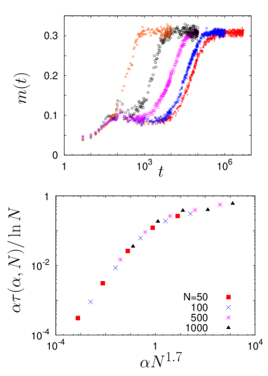
Figure 16: (Upper panel) Magnetization versus time for $N=500$ at $\varepsilon=0.69$ and for $\alpha$ values (right to left) $10^{-6},10^{-5},10^{-4},10^{-3}$, and $10^{-2}$. With increasing $\alpha$, one can observe a faster relaxation towards equilibrium. (Lower panel) $\alpha\tau(\alpha,N)/\ln N$ versus $\alpha N^{\gamma}$, showing scaling collapse in accordance with Eq. (101). Here, we have $\varepsilon=0.69$.

For $\alpha^{-1}\ll N^{\gamma}$, and times $\alpha^{-1}\ll t\ll N^{\gamma}$, the system size is effectively infinite and the evolution follows the Boltzmann equation. Here, frequent collisions at short times drive the momentum distribution towards a Gaussian. As noted above, until this happens, the initial magnetization does not change in time. Over the time the momentum distribution becomes Gaussian, the instability of such a state under the Boltzmann equation leads to a fast relaxation towards equilibrium, similar to the result for the Vlasov-unstable regime. The asymptotic behavior of the magnetization is thus

$$m(t)\sim\frac{1}{\sqrt{N}}e^{\alpha t};~{}N^{\gamma}\gg t\gg\alpha^{-1}.$$ (99)

By requiring that $m(t)$ acquires a value of $O(1)$, the above equation gives the relaxation time $\tau_{\mathrm{S}}$, determined by the stochastic process, as $\tau_{\mathrm{S}}\sim\ln N/\alpha$. In the opposite limit, $\alpha^{-1}\gg N^{\gamma}$, collisions are infrequent, and therefore, the process that drives the momentum distribution to a Gaussian is delayed. The magnetization stays close to its initial value, and relaxes only over the time $\sim N^{\gamma}$, over which finite-size effects come into play. Here, similar to the result for the Vlasov-stable regime, the magnetization at late times behaves as

$$m(t)\sim\frac{1}{\sqrt{N}}e^{t/N^{\gamma}};~{}\alpha^{-1}\gg t\gg N^{\gamma}.$$ (100)

This equation gives the relaxation time $\tau_{\mathrm{D}}$, determined by the deterministic process, as $\tau_{\mathrm{D}}\sim N^{\gamma}\ln N$. Interpolating between the above two limits of the timescales, one expects the relaxation time $\tau(\alpha,N)$ to obey $\tau^{-1}=\tau_{\mathrm{S}}^{-1}+\tau_{\mathrm{D}}^{-1}$, yielding $\tau(\alpha,N)\sim\ln N/(\alpha+1/N^{\gamma})$. More generally, this suggests a scaling form

$$\tau(\alpha,N)\sim\frac{\ln N}{\alpha}g(\alpha N^{\gamma}),$$ (101)

where, consistent with Eqs. (99) and (100), the scaling function $g(x)$ behaves as follows: $g(x)\sim x$ for $x\ll 1$, while $g(x)\rightarrow$ constant for $x\gg 1$. Equation (101) implies that for fixed $N$, the relaxation time of the water-bag initial state exhibits a crossover, from being of order $N^{\gamma}\ln N$ (corresponding to QSSs) for $\alpha\ll 1/N^{\gamma}$ to being of order $\ln N$ for $\alpha\gg 1/N^{\gamma}$. This brings us to the main conclusion of this Subsection: In the presence of collisions, the relaxation at long times does not occur over an algebraically growing timescale, which implies that under noisy microcanonical evolution, QSSs occur only as a crossover phenomenon and are lost in the limit of long times.

The above predictions, in particular, the scaling form in Eq. (101), may be verified by performing extensive numerical simulations of the generalized HMF model. The Hamilton equations, Eq. (90), may be integrated by using a symplectic fourth-order integrator. In realizing the stochastic process $(p,p^{\prime},p^{\prime\prime})\rightarrow(q,q^{\prime},q^{\prime\prime})$ while conserving the three-particle energy $E$ and momentum $P$, we note that the updated momenta lie on a circle formed by the intersection of the plane $p+p^{\prime}+p^{\prime\prime}=P$ and the spherical surface $p^{2}+p^{\prime 2}+p^{\prime\prime 2}=2E$. The radius of this circle is given by $r=\sqrt{2E-P^{2}/3}$. The new momenta may thus be parametrized in terms of an angle $\phi$ measured along this circle, as $q=(P/\sqrt{3})+r\sqrt{2/3}\cos\phi,q^{\prime}=(P/\sqrt{3})-(r/\sqrt{6})\cos\phi-(r/\sqrt{2})\sin\phi,q^{\prime\prime}=(P/\sqrt{3})-(r/\sqrt{6})\cos\phi+(r/\sqrt{2})\sin\phi$. Stochasticity in updates is achieved through choosing the angle $\phi$ uniformly in $[0,2\pi)$. Following the foregoing scheme, typical time evolution of the magnetization in the generalized HMF model for $N=500$ and several values of $\alpha$ at an energy density $\varepsilon=0.69$ are shown in Fig. 16(Upper panel). The relaxation time $\tau(\alpha,N)$ is taken as the time for the magnetization to reach the fraction $0.8$ of the final equilibrium value (the result, however, is not sensitive to this choice). At $\varepsilon=0.69$, where the equilibrium value of the magnetization is $\simeq 0.3$ and $\gamma\simeq 1.7$, we plot $\alpha\tau(\alpha,N)/\ln N$ versus $\alpha N^{\gamma}$ to check the scaling form in Eq. (101). Figure 16(Lower panel) shows an excellent scaling collapse over several decades; this is consistent with our prediction for QSSs as a crossover phenomenon under noisy microcanonical dynamics.

6.2 HMF model generalized to particles moving on a sphere

In order to probe the ubiquity of the quasistationary behavior observed in the HMF model, various extensions of the model have been introduced and analyzed over the years. For example, the HMF model was considered with an additional term in the energy that is due to either (i) a global anisotropy in the magnetization along the $x$-axis, or, (ii) an onsite potential. In either case, QSSs were shown to exist in specific energy ranges, with a relaxation time scaling algebraically with the system size. A particularly interesting generalization of the HMF model is to that of particles moving on the surface of a sphere rather than on a circle [28]: Consider a system of $N$ interacting particles moving on the surface of a unit sphere. The generalized coordinates of the $i$-th particle are the spherical polar angles $\theta_{i}\in[0,\pi]$ and $\phi_{i}\in[0,2\pi]$, while the corresponding generalized momenta are $p_{\theta_{i}}$ and $p_{\phi_{i}}$. The Hamiltonian of the system is given by

$$H=\frac{1}{2}\sum_{i=1}^{N}\Big{(}p_{\theta_{i}}^{2}+\frac{p_{\phi_{i}}^{2}}{\sin^{2}\theta_{i}}\Big{)}+\frac{1}{2N}\sum_{i,j=1}^{N}\Big{[}1-{\bf S}_{i}\cdot{\bf S}_{j}\Big{]}.$$ (102)

Here, ${\bf S}_{i}$ is the vector pointing from the center to the position of the $i$-th particle on the sphere, and has the Cartesian components $(S_{ix},S_{iy},S_{iz})=(\sin\theta_{i}\cos\phi_{i},\sin\theta_{i}\sin\phi_{i},\cos\theta_{i})$. Regarding the vector ${\bf S}_{i}$ as the classical Heisenberg spin vector of unit length, the interaction term in Eq. (102) has a form similar to that in a mean-field Heisenberg model of magnetism. However, unlike the latter case, the Poisson bracket between the components of ${\bf S}_{i}$’s is identically zero. Relative to the HMF model, the model (102) is defined on a larger phase space with each particle characterized by two positional degrees of freedom rather than one.

The interaction term in Eq. (102) tries to cluster the particles, and is in competition with the kinetic energy term (the term involving $p_{\theta_{i}}$ and $p_{\phi_{i}}$) that has the opposite effect. The degree of clustering is conveniently measured by the “magnetization” vector ${\bf m}=(m_{x},m_{y},m_{z})\equiv\sum_{i=1}^{N}{\bf S}_{i}/N$. In the BG equilibrium state, the system exhibits a continuous phase transition at the critical energy density $\varepsilon_{c}\equiv 5/6$, between a low-energy clustered (“magnetized”) phase in which the particles are close together on the sphere, and a high-energy homogeneous (“non-magnetized”) phase in which the particles are uniformly distributed on the sphere. As a function of the energy, the magnitude of ${\bf m}$, i.e., $m=\sqrt{m_{x}^{2}+m_{y}^{2}+m_{z}^{2}}$, decreases continuously from unity at zero energy density to zero at $\varepsilon_{c}$, and remains zero at higher energies. The mentioned phase transition properties may be derived by following a procedure similar to the one invoked in Section 5.

The time evolution of the system (102) follows the usual Hamilton equations of motion derived from the Hamiltonian (102). The issue of how the system while starting far from equilibrium and evolving under the Hamilton equations relaxes to the equilibrium state may be investigated by studying the Vlasov equation for the evolution of the single-particle phase space density. Let $f(\theta,\phi,p_{\theta},p_{\phi},t)$ be the probability density in this phase space, such that $f(\theta,\phi,p_{\theta},p_{\phi},t){\rm d}\theta{\rm d}\phi{\rm d}p_{\theta}{\rm d}p_{\phi}$ gives the probability at time $t$ to find the particle with its generalized coordinates in $(\theta,\theta+{\rm d}\theta)$ and $(\phi,\phi+{\rm d}\phi)$, and the corresponding momenta in $(p_{\theta},p_{\theta}+{\rm d}p_{\theta})$ and $(p_{\phi},p_{\phi}+{\rm d}p_{\phi})$. The Vlasov equation reads [28]

$$\frac{\partial f}{\partial t}+p_{\theta}\frac{\partial f}{\partial\theta}+\frac{p_{\phi}}{\sin^{2}\theta}\frac{\partial f}{\partial\phi}+\Big{(}\frac{p^{2}_{\phi}\cos\theta}{\sin^{3}\theta}+m_{x}\cos\theta\cos\phi+m_{y}\cos\theta\sin\phi-m_{z}\sin\theta\Big{)}\frac{\partial f}{\partial p_{\theta}}$$

$$+(-m_{x}\sin\theta\sin\phi+m_{y}\sin\theta\cos\phi)\frac{\partial f}{\partial p_{\phi}}=0;$$ (103)

$$(m_{x},m_{y},m_{z})=\int{\rm d}\theta{\rm d}\phi{\rm d}p_{\theta}{\rm d}p_{\phi}~{}(\sin\theta\cos\phi,\sin\theta\sin\phi,\cos\theta)f.$$ (104)

It is easily verified that any distribution $f^{(0)}(\theta,\phi,p_{\theta},p_{\phi})=\Phi(e(\theta,\phi,p_{\theta},p_{\phi}))$, with arbitrary function $\Phi$, and $e$ being the single-particle energy,

$$e(\theta,\phi,p_{\theta},p_{\phi})=\frac{1}{2}\Big{(}p_{\theta}^{2}+\frac{p_{\phi}^{2}}{\sin^{2}\theta}\Big{)}-m_{x}\sin\theta\cos\phi-m_{y}\sin\theta\sin\phi-m_{z}\cos\theta,$$ (105)

is stationary under the Vlasov dynamics (103). The magnetization components $m_{x},m_{y},m_{z}$ are determined self-consistently. As a specific example, consider a stationary state that is non-magnetized, that is, $m_{x}=m_{y}=m_{z}=0$, and $f^{(0)}(\theta,\phi,p_{\theta},p_{\phi})$ is given by

$$f^{(0)}(\theta,\phi,p_{\theta},p_{\phi})=\left\{\begin{array}[]{ll}&\frac{1}{2\pi}\frac{1}{\pi}A\mbox{~{}~{}if~{}}\frac{1}{2}\Big{(}p_{\theta}^{2}+\frac{p_{\phi}^{2}}{\sin^{2}\theta}\Big{)}<E;\\ &\theta\in[0,\pi],\phi\in[0,2\pi],A,E\geq 0,\\ &0,\mbox{~{}~{}~{}~{}~{}~{}~{}~{}otherwise}.\end{array}\right.\\$$ (106)

The state (106) is a straightforward generalization of the water-bag initial condition for the HMF model. The parameters $A$ and $E$ are related through the normalization condition, $\int_{0}^{\pi}{\rm d}\theta\int_{0}^{2\pi}{\rm d}\phi\int_{\Omega}{\rm d}p_{\theta}{\rm d}p_{\phi}f^{(0)}=1$, where the integration over $p_{\theta}$ and $p_{\phi}$ is over the domain $\Omega\equiv\Theta\Big{(}2E-p_{\theta}^{2}-p_{\phi}^{2}/\sin^{2}\theta\Big{)}$, with $\Theta(x)$ denoting the unit step function. One gets $E=1/(4A)$, while the conserved energy density $\varepsilon=1/2+\int_{0}^{\pi}{\rm d}\theta\int_{0}^{2\pi}{\rm d}\phi\int_{\Omega}{\rm d}p_{\theta}{\rm d}p_{\phi}(1/2)\Big{(}p_{\theta}^{2}+p_{\phi}^{2}/\sin^{2}\theta\Big{)}f^{(0)}$ is related to $E$ as $\varepsilon=(E+1)/2$.

Analyzing the linear stability of the stationary state (106) under the Vlasov dynamics (103), it may be shown that for energies $\varepsilon>\varepsilon^{*}=2/3$, the non-magnetized state (106) is linearly stable, and is hence a QSS. In a finite system, the QSS eventually relaxes to BG equilibrium over a very long timescale, which, considering the magnetization as an indicator for the relaxation process for energies $\varepsilon<\varepsilon_{c}$, grows algebraically with the system size as $N^{\gamma};~{}\gamma>0$; this is demonstrated by numerical simulation results in Fig. 17. For energies $\varepsilon<\varepsilon^{*}$, the state (106) is linearly unstable, and is thus not a QSS; in this case, numerical simulations show that the system exhibits a fast relaxation towards BG equilibrium over a timescale that grows with the system size as $\ln N$. These features of a linearly unstable and a linear stable regime of a non-magnetized Vlasov-stationary state, with a QSS emerging in the latter case, remain unaltered on adding a term to the Hamiltonian (102) that accounts for a global anisotropy in the magnetization. We note that a non-mean-field version of the model was studied in Ref. [29] in the context of the existence of QSSs.

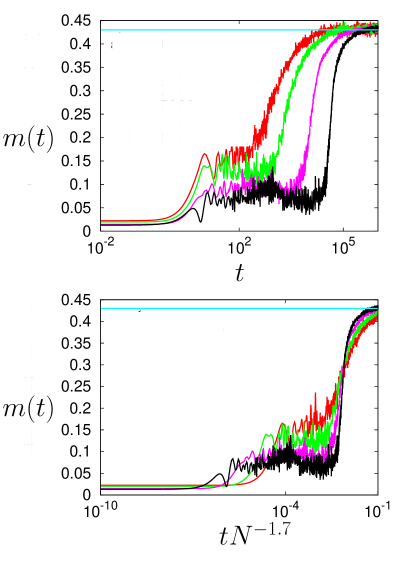
Figure 17: For the model (102), the figures show numerical simulation results for the magnetization $m(t)$ as a function of time (Upper panel), and as a function of time scaled by $N^{1.7}$ (Lower panel) in the Vlasov-stable phase ($\varepsilon>\varepsilon^{*}$). The energy density is $\varepsilon=0.7$. The blue line indicates the BG equilibrium value. The figures suggest the existence of a QSS with a lifetime scaling with the system size as $N^{1.7}$.

6.3 A long-range model of spins

The ubiquity of QSSs may be tested in a dynamics very different from the particle dynamics of either the HMF model or any of its generalizations, including the model (102), namely, within classical spin dynamics of an anisotropic Heisenberg model with mean-field interactions [30, 31]. The model comprises $N$ globally coupled three-component Heisenberg spins of unit length, ${\mathbf{S}}_{i}=(S_{ix},S_{iy},S_{iz})$, $i=1,2,\ldots,N$. In terms of spherical polar angles $\theta_{i}\in[0,\pi]$ and $\phi_{i}\in[0,2\pi]$ for the orientation of the $i$-th spin, one has $S_{ix}=\sin\theta_{i}\cos\phi_{i},S_{iy}=\sin\theta_{i}\sin\phi_{i},S_{iz}=\cos\theta_{i}$. The Hamiltonian of the model is given by

$$H=-\frac{J}{2N}\sum_{i,j=1}^{N}{\bf S}_{i}\cdot{\bf S}_{j}+D\sum_{i=1}^{N}S^{2}_{iz},$$ (107)

where the first term with $J>0$ describes a ferromagnetic mean-field like coupling, while the last term gives the energy due to a local anisotropy. We take $D>0$ such that at equilibrium, the energy is lowered by having the magnetization ${\bf m}\equiv(1/N)\sum_{i=1}^{N}{\bf S}_{i}$ pointing in the $xy$ plane. The model (107) has an equilibrium phase diagram with a continuous transition from a low-energy magnetic phase ($m\neq 0$) to a high-energy non-magnetic phase ($m=0$) across the critical energy density $\varepsilon_{c}=D\left(1-2/\beta_{c}\right)$, where $\beta_{c}$ satisfies $2/\beta_{c}=1-1/(2\beta_{c}D)+\exp(-\beta_{c}D)/(\sqrt{\pi\beta_{c}D}\mathrm{Erf}[\sqrt{\beta_{c}D}])$, with ${\rm Erf}(x)$ being the error function. The derivation of these properties is detailed in Ref. [30].

The time evolution of the model (107) is governed by the set of equations

$$\frac{{\rm d}{\bf S}_{i}}{{\rm d}t}=\{{\bf S}_{i},H\};~{}~{}~{}~{}i=1,2,\ldots,N.$$ (108)

Here the Poisson bracket $\{A,B\}$ for two functions of the spins is obtained by noting that suitable canonical variables for a classical spin are $\phi$ and $S_{z}$, so that in our model, $\{A,B\}\equiv\sum_{i=1}^{N}(\partial A/\partial\phi_{i}\partial B/\partial S_{iz}-\partial A/\partial S_{iz}\partial B/\partial\phi_{i})=\sum_{i=1}^{N}{\bf S}_{i}\cdot\partial A/\partial{\bf S}_{i}\times\partial B/\partial{\bf S}_{i}$, using which one obtains straightforwardly

$$\frac{{\rm d}S_{ix}}{{\rm d}t}=S_{iy}m_{z}-S_{iz}m_{y}-2DS_{iy}S_{iz},$$ (109)

$$\frac{{\rm d}S_{iy}}{{\rm d}t}=S_{iz}m_{x}-S_{ix}m_{z}+2DS_{ix}S_{iz},$$ (110)

$$\frac{{\rm d}S_{iz}}{{\rm d}t}=S_{ix}m_{y}-S_{iy}m_{x}.$$ (111)

From Eq. (111), one finds by summing over $i$ that $m_{z}$ is a constant of motion. The motion also conserves the total energy and the length of each spin.

To study the relaxation to equilibrium while starting far from it, one analyzes as usual the Vlasov equation for the evolution of the single-spin phase space density. Denoting the latter by $f(\theta,\phi,t)$, with $f(\theta,\phi,t)\sin\theta{\rm d}\theta{\rm d}\phi$ giving the probability to find a spin with its angles between $\theta$ and $\theta+{\rm d}\theta$ and between $\phi$ and $\phi+{\rm d}\phi$ at time $t$, the Vlasov equation may be shown to be of the form [30]

$$\frac{\partial f}{\partial t}=\Big{[}m_{y}\cos\phi-m_{x}\sin\phi\Big{]}\frac{\partial f}{\partial\theta}-\Big{[}m_{x}\cot\theta\cos\phi+m_{y}\cot\theta\sin\phi-m_{z}+2D\cos\theta\Big{]}\frac{\partial f}{\partial\phi}.$$ (112)

In the above equation, the magnetization components are given by $(m_{x},m_{y},m_{z})=\int\sin\theta^{\prime}{\rm d}\theta^{\prime}{\rm d}\phi^{\prime}(\sin\theta^{\prime}\cos\phi^{\prime},\sin\theta^{\prime}\sin\phi^{\prime},\cos\theta^{\prime})f(\theta^{\prime},\phi^{\prime},t)$.

Consider an initial state prepared by sampling independently for each of the $N$ spins the angle $\phi$ uniformly over $[0,2\pi]$ and the angle $\theta$ uniformly over an arbitrary interval symmetric about $\pi/2$. Such a state will have the distribution

$$f(\theta,\phi,0)=\frac{1}{2\pi}p(\theta),$$ (113)

with $p(\theta)$, the distribution for $\theta$, given by

$$p(\theta)=\left\{\begin{array}[]{ll}\frac{1}{2\sin a}&\mbox{if $\theta\in\left[\frac{\pi}{2}-a,\frac{\pi}{2}+a\right]$},\\ &\\ 0&\mbox{otherwise}.\end{array}\right.\\$$ (114)

Here, $a>0$ is a given parameter. The state (113) is analogous to the water-bag state studied in the context of the HMF model. It is easily verified that this non-magnetic state has the energy $\varepsilon=(D/3)\sin^{2}a$, and that the state is stationary under the Vlasov dynamics (112).

A linear stability analysis of the state (113) under the Vlasov dynamics (112) shows that the state is linearly stable for energies $\varepsilon>\varepsilon^{*}\equiv D/(3+12D)$, and is thus a QSS. In this case, in a finite system, such a state eventually relaxes to BG equilibrium; studying the time evolution of the magnetization to monitor this relaxation for energies $\varepsilon<\varepsilon_{c}$, it may be seen that the relaxation occurs on a timescale $\sim N^{\gamma}$, with $\gamma>0$, see Fig. 18. A detailed analytical study of the Lenard-Balescu operator that accounts at leading order for the finite-size effects driving the relaxation of the QSSs was taken up in Ref. [31], and it was demonstrated that indeed corrections at leading order are identically zero, so that relaxation has to occur over a time longer than of order $N$, in agreement with the numerical results. For $\varepsilon<\varepsilon^{*}$, when the water-bag state is linearly unstable, the magnetization shows a relaxation from the initial value over a timescale $\tau(N)\sim\ln N$, see Ref. [30].

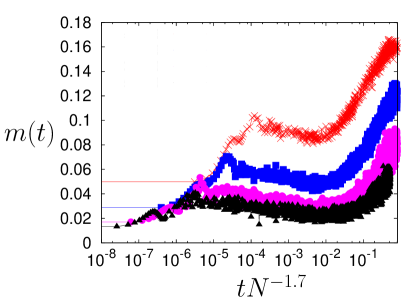
Figure 18: For the model (107), the figure shows numerical simulation results for the magnetization $m(t)$ as a function of $tN^{-1.7}$ with energy density $\varepsilon=0.24>\varepsilon^{*}$, the parameter $D=15$, and for systems of size $N=300,1000,3000,5000$ (top to bottom). The figure suggests a QSS life-time $\tau(N)\sim N^{1.7}$.

7 Driving a long-range system out of thermal equilibrium: Temperature inversion and cooling

What happens when an isolated macroscopic long-range system in thermal equilibrium is momentarily disturbed, e.g., by an impulsive force or a “kick”? How different from an equilibrium state is the stationary state the system relaxes to after the kick? Are there ways to characterize it, e.g., by unveiling some of its general features? These questions were addressed in detail in a recent series of papers [32, 33, 34, 35], demonstrating that when the equilibrium state is spatially inhomogeneous, the system after the kick relaxes to a QSS that is characterized by a non-uniform temperature profile in space. In short-range systems, by contrast, a non-uniform temperature profile may only occur when the system is actively maintained out of equilibrium, e.g., by a boundary-imposed temperature gradient, to counteract collisional effects. In addition to a non-uniform temperature profile, in a long-range system, the QSS attained following the kick generically exhibits a remarkable phenomenon of temperature inversion. Namely, the temperature and density profiles as a function of space are anticorrelated, that is, denser parts of the system are colder than dilute ones. Temperature inversion is observed in nature, e.g., in interstellar molecular clouds and especially in the solar corona, where temperatures around $10^{6}$ K that are three orders of magnitude larger than the temperature of the photosphere are attained.

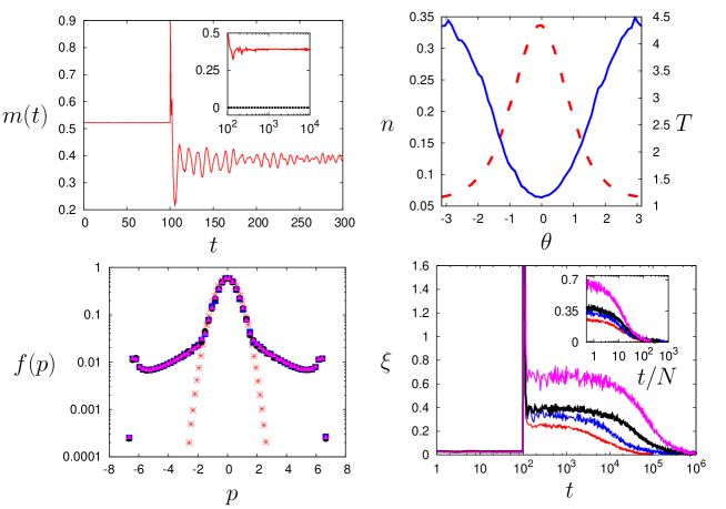
Figure 19: In the HMF model, while starting with thermal equilibrium at temperature $T=0.4244$ with corresponding equilibrium magnetization $m_{x}=0.521$ and $m_{y}=0$, the system is let evolve until $t=t_{0}=100$, and then kicked out of equilibrium by applying an external magnetic field $h=10.0$ along the $x$ direction for times $t_{0}<t<t_{0}+1$. The first three panels show molecular dynamics simulation results for $N=10^{7}$ for (First panel) Time evolution of the magnetization $m$ (solid red line); here the inset shows for longer times $m(t)$ compared to the equilibrium value $m_{\text{eq}}=0$ (dotted black line) at the same energy; (Second panel) Temperature profile $T(\theta)$ (blue solid line) and density profile $n(\theta)$ (red dashed line) measured in the QSS obtained at $t=10^{4}$; (Third panel) Momentum distribution $f(p)$ at $t=0$ (red crosses), $t=5\times 10^{2}$ (blue squares), $t=10^{3}$ (black circles), $t=10^{4}$ (purple triangles); that the distributions for the last three cases are indistinguishable implies that the system is in a stationary state (and is in fact in a QSS, see discussions in the main text). The fourth panel shows time evolution of the space-integrated distance $\xi$ of the instantaneous temperature from the equilibrium temperature at the same energy, for different values of $N$ increasing from bottom to top as $N=5\times 10^{2}$ (red), $N=10^{3}$ (blue), $N=2.5\times 10^{3}$ (black), $N=5\times 10^{3}$ (purple). The inset of the fourth panel shows $\xi$ as a function of $t/N$.

To demonstrate the claim of temperature inversion, the dynamical evolution of the HMF system kicked out of thermal equilibrium may be studied via molecular dynamics (MD) simulations involving numerical integration of its equations of motion. As an illustrative example, the system is initially prepared in thermal equilibrium at temperature $T=0.4244$ with corresponding equilibrium magnetization $m_{x}=m_{0}=0.521$ and $m_{y}=0$, let evolve until $t=t_{0}>0$, and then kicked out of equilibrium by applying during a short time $\tau$ an external magnetic field $h$ along the $x$ direction; thus, for $t_{0}<t<t_{0}+\tau$, the Hamiltonian (79) is augmented by the term $H_{h}=-h\sum_{i=1}^{N}\cos\theta_{i}$. Here, we present results for $t_{0}=100$, $\tau=1$, $h=10$, and $N=10^{7}$. After the kick, the magnetization starts oscillating, but eventually damps down to a stationary value smaller than $m_{0}$. A typical time evolution of the magnetization is shown in Fig. 19, First panel. The stationary state reached after the damping of the oscillations is a QSS. The nonequilibrium character of this state is shown by the fact that the temperature profile

$$T(\theta)\equiv\frac{\int_{-\infty}^{\infty}dp\,p^{2}f(\theta,p)}{\int_{-\infty}^{\infty}dp\,f(\theta,p)}$$ (115)

is non-uniform, and there is temperature inversion, as shown in Fig. 19, Second panel, where $T(\theta)$ is plotted together with the density profile

$$n(\theta)\equiv\int_{-\infty}^{\infty}dp\,f(\theta,p).$$ (116)

Here, $f(\theta,p)$ is the usual single-particle phase space density. The temperature profile indeed remains essentially the same for the whole lifetime of the QSS, as may be checked by measuring an integrated distance $\xi$ between the actual temperature profile and the constant equilibrium one, $T_{\text{eq}}$, at the same energy, as follows:

$$\xi(t)\equiv\int_{-\pi}^{\pi}\left|T(\theta,t)-T_{\text{eq}}\right|d\theta.$$ (117)

In Fig. 19, Third panel, we show that the momentum distribution in the QSS reached after the kick develops supra-thermal tails, while in the fourth panel, $\xi(t)$ is plotted for systems with different values of $N$ kicked with the same $h=10$ at $t_{0}=100$ for a duration $\tau=1$. After the kick, $\xi(t)$ oscillates and then reaches a plateau whose duration grows with $N$, as expected for a QSS. The inset of Fig. 19, Fourth panel, shows that if times are scaled by $N$, the curves reach zero at the same time, consistently with the lifetime of an inhomogeneous QSS being proportional to $N$.

8 Conclusions

In this brief contribution, we offered an overview of properties of long-range interacting (LRI) systems. We exclusively focussed on systems for which the long-time stationary state is in equilibrium. Because of lack of space, we could not cover the even richer static and dynamics properties exhibited by systems that have a non-equilibrium stationary state [36, 37, 38, 39, 40, 41, 42, 43, 44, 45]. LRI systems present a particularly exciting area of research due to the possibility to develop theoretical tools that effectively combine and adapt methods and techniques from diverse fields, but also in the wake of new experimental realizations of LRI systems that offer the possibility to directly test the predictions obtained in theory. We hope that this contribution will serve as an invitation to young (and old) minds to delve into the exciting world of long-range interactions.

References

- [1] Dynamics and Thermodynamics of Systems with Long-Range Interactions, Lecture Notes in Physics, vol. 602, edited by T. Dauxois, S. Ruffo, E. Arimondo, and M. Wilkens (Springer, Berlin, 2002).
- [2] Dynamics and Thermodynamics of Systems with Long-range Interactions: Theory and Experiment, edited by A. Campa, A. Giansanti, G. Morigi, and F. Sylos Labini, AIP Conference Proceedings 970 (2008).
- [3] S. Ruffo, Eur. Phys. J. B 64, 355 (2008).
- [4] A. Campa, T. Dauxois, and S. Ruffo, Phys. Rep. 480, 57 (2009).
- [5] Long-range interacting systems, edited by T. Dauxois, S. Ruffo, and L. Cugliandolo (Oxford University Press, Oxford, 2009).
- [6] F. Bouchet, S. Gupta, and D. Mukamel, Physica A 389, 4389 (2010).
- [7] Journal of Statistical Mechanics: Theory and Experiment Topical issue: Long-Range Interacting Systems, edited by T. Dauxois and S. Ruffo (2010).
- [8] A. Campa, T. Dauxois, D. Fanelli, and S. Ruffo, Physics of Long-Range Interacting Systems, (Oxford University Press, Oxford, 2014)
- [9] M. Kiessling and J. L. Lebowitz, Letters in Mathematical Physics 42, 43 (1997).
- [10] J. Barré, D. Mukamel, and S. Ruffo, Phys. Rev. Lett. 87, 030601 (2001).
- [11] R. S. Ellis, K. Haven, and B. Turkington, Nonlinearity 15, 239 (2002).
- [12] A. Pikovsky, S. Gupta, T. N. Teles, F. P. C. Benetti, R. Pakter, Y. Levin, and S. Ruffo, Phys. Rev. E 90, 062141 (2014).
- [13] D. H. E. Dubin, in Long-Range Interacting Systems, edited by T. Dauxois, S. Ruffo, and L. F. Cugliandolo (Oxford University Press, Oxford, 2010).
- [14] S. T. Bramwell, in Long-Range Interacting Systems, edited by T. Dauxois, S. Ruffo, and L. F. Cugliandolo (Oxford University Press, Oxford, 2010).
- [15] J. Barré, T. Dauxois, G. De Ninno, D. Fanelli, and S. Ruffo, Phys. Rev. E 69, 045501 (R) (2004).
- [16] P.-H. Chavanis, in Dynamics and Thermodynamics of Systems with Long-range Interactions: Theory and Experiment, edited by A. Campa, A. Giansanti, G. Morigi, and F. Sylos Labini, AIP Conference Proceedings 970 (2008).
- [17] D. Mukamel, S. Ruffo, and N. Schreiber, Phys. Rev. Lett. 95, 240604 (2005).
- [18] M. Antoni and S. Ruffo, Phys. Rev. E 52, 2361 (1995).
- [19] Y. Y. Yamaguchi, J. Barré, F. Bouchet, T. Dauxois, and S. Ruffo, Physica A 337, 36 (2004).
- [20] Y. Levin, R. Pakter, F. B. Rizzato, T. N. Teles, and F. P. da C. Benetti, Phys. Rep. 535 1 (2014).
- [21] C. Anteneodo and C. Tsallis, Phys. Rev. Lett. 80, 5313 (1998).
- [22] S. Gupta, A. Campa, and Stefano Ruffo, Phys. Rev. E 86, 061130 (2012).
- [23] S. Schütz and G. Morigi, Phys. Rev. Lett. 113, 203002 (2014).
- [24] S. Schütz, S. B. Jäger, and G. Morigi, Phys. Rev. Lett. 117, 083001 (2016).
- [25] S. B. Jäger, S. Schütz, and G. Morigi, Phys. Rev. A 94, 023807 (2016).
- [26] S. Gupta and D. Mukamel, Phys. Rev. Lett. 105, 040602 (2010).
- [27] S. Gupta and D. Mukamel, J. Stat. Mech.: Theory Exp. P08026 (2010).
- [28] S. Gupta and D. Mukamel, Phys. Rev. E 88, 052137 (2013).
- [29] L. J. L. Cirto, L. S. Lima, and F. D Nobre, J. Stat. Mech.: Theory Exp. P04012 (2015).
- [30] S. Gupta and D. Mukamel, J. Stat. Mech.: Theory Exp. P03015 (2011).
- [31] J. Barré and S. Gupta, J. Stat. Mech.: Theory Exp. P02017 (2014).
- [32] L. Casetti and S. Gupta, Eur. Phys. J. B 87, 91 (2014).
- [33] T. N. Teles, S. Gupta, P. D. Cintio, and L. Casetti, Phys. Rev. E 92, 020101(R) (2015).
- [34] T. N. Teles, S. Gupta, P. D. Cintio, and L. Casetti, Phys. Rev. E 93, 066102 (2016).
- [35] S. Gupta and L. Casetti, New J. Phys. 18, 103051 (2016).
- [36] C. Nardini, S. Gupta, S. Ruffo, T. Dauxois, and F. Bouchet, J. Stat. Mech.: Theory Exp. L01002 (2012).
- [37] S. Gupta, M. Potters, and S. Ruffo, Phys. Rev. E 85, 066201 (2012).
- [38] C. Nardini, S. Gupta, S. Ruffo, T. Dauxois, and F. Bouchet, J. Stat. Mech.: Theory Exp. P12010 (2012).
- [39] S. Gupta, A. Campa, and S. Ruffo, Phys. Rev. E 89, 022123 (2014).
- [40] S. Gupta, T. Dauxois, and S. Ruffo, J. Stat. Mech.: Theory Exp. P11003 (2013).
- [41] M. Komarov, S. Gupta, and A. Pikovsky, EPL 106, 40003 (2014).
- [42] S. Gupta, A. Campa, and S. Ruffo, J. Stat. Mech.: Theory Exp. R08001 (2014).
- [43] A. Campa, S. Gupta, and S. Ruffo, J. Stat. Mech.: Theory Exp. P05011 (2015).
- [44] S. Gupta, T. Dauxois, and S. Ruffo, EPL 113, 60008 (2016).
- [45] A. Campa and S. Gupta, EPL 116, 30003 (2016).