Renormalization of scalar field theories in rational spacetime dimensions

Abstract. We renormalize various scalar field theories with a $\phi^{n}$ self interaction such as $n$ $=$ $5$, $7$ and $9$ in their respective critical dimensions which are non-integer. The renormalization group functions for the $O(N)$ symmetric extensions are also computed.

LTH 1130

1 Introduction.

Scalar quantum field theories have provided an excellent laboratory for many years to explore and test ideas in physical problems. For instance, the development of Wilson’s renormalization group and its application to theories defined close to an integer spacetime dimension led to the concept of the Wilson-Fisher fixed point, [1, 2, 3, 4, 5]. Being defined as a non-trivial zero of the $\beta$-functions in spacetime dimensions $d$ $=$ $D_{n}$ $-$ $2\epsilon$, where $D_{n}$ is the critical dimension which will be defined later for a scalar theory and is not necessarily an integer, meant that the renormalization group functions in the neighbourhood of a fixed point provided information on phase transitions in nature, [1, 2, 5]. A widely studied example is that of the Ising model which can be described by scalar $\phi^{4}$ theory. In this case $D_{n}$ $=$ $4$, while other theories such as scalar $\phi^{3}$ have $D_{n}$ $=$ $6$ and this potential underpins the properties of phase transitions for other phenomena. For example, the Lee-Yang singularity problem can be accessed via $\phi^{3}$ theory. Recently there has been renewed interest in examining scalar $\phi^{n}$ theories for $n$ $\geq$ $4$. Early work on such higher order potentials included articles on $\phi^{6}$ theory, [6, 7, 8, 9, 10, 11, 12], and $\phi^{2r}$ potentials for integer $r$, [13, 14]. However, more recently scalar $\phi^{5}$ theory was studied in [15] using the functional renormalization group method as well as via critical exponents in [16, 17, 18]. The motivation was to develop and investigate the continuum quantum field theory for the Blume-Capel universality class which is the next after the Ising and Lee-Yang classes. Equally as phase transitions have scale and conformal symmetry, the formalism of conformal field theory has been used to calculate exponents and central charges associated with the correlation functions of various operators or currents, [17, 18, 19, 20]. These were then used to inform the structure of the perturbative renormalization group functions. One aim is partly to continue building up the formalism associated with $d$-dimensional conformal field theory as well as to have a powerful tool to make predictions for new universality classes such as the Blume-Capel one.

Given this resurgence of interest in scalar field theories with higher order potentials there is a clear need to complement the conformal field theory approach with explicit perturbative computations. This is the purpose of this article. Aside from $\phi^{4}$ and $\phi^{3}$ theories whose renormalization group functions are known to high order, [21, 22, 23, 24, 25, 26, 27, 28, 29, 30, 31, 32, 33, 34], only $\phi^{6}$ theory has been renormalized to any depth, [8, 9, 12]. Some leading order results are available for $\phi^{2r}$ theories for integer $r$ $\geq$ $4$ but those for potentials with odd powers except $3$ are virtually unknown. Therefore we will consider the $\phi^{5}$, $\phi^{7}$ and $\phi^{9}$ scalar field theories and determine the anomalous dimensions and $\beta$-functions as well as those for $\phi^{8}$ for a reason which will become apparent later. While this is simple to state it is worth observing that these scalar theories are not renormalizable in integer dimensions. By contrast their critical dimension is rational. Although this is clearly not a value for a physical spacetime such models should in principle provide more accurate predictions for physical phase transitions. As has been noted for example in [15] if the critical dimension is close to an integer then the use of $d$ $=$ $D_{n}$ $-$ $2\epsilon$ means that choosing a small value of $\epsilon$ in the $\epsilon$-expansion of the first few terms of a critical exponent should yield accurate exponent estimates in that integer dimension. This is in contrast with the use of the $\epsilon$-expansion in $\phi^{4}$ theory where $d$ $=$ $4$ $-$ $2\epsilon$ and $d$ has to be $3$ for Ising model predictions which requires the relatively high value of $\epsilon$ $=$ $\frac{1}{2}$. In this context $\phi^{4}$ theory can also be used to access other physical phenomena if it is endowed with an $O(N)$ symmetry. Then, for instance, $N$ $=$ $2$ describes superfluidity while $N$ $=$ $3$ corresponds to the Heisenberg magnet. Therefore in this spirit we will extend the odd higher potentials to include an $O(N)$ symmetry and compute the corresponding renormalization group functions. This leads to an interesting prospect which may connect the $O(N)$ $\phi^{5}$ and $O(N)$ $\phi^{8}$ theories with potentially a generalization for higher order potentials. Such connections should be established by explicit computations. For the widely known ultraviolet completion of $O(N)$ $\phi^{4}$ theory in four dimensions to $O(N)$ $\phi^{3}$ theory in six dimensions, [33, 35], this has been put on a concrete foundation via higher order perturbative computations and the large $N$ expansion. Equally the $d$-dimensional conformal field theory formalism is in a position to address the same connection in principle. Hence it ought to be a crucial tool for the new connections that we suggest are apparent here in the higher order potentials. Therefore providing renormalization group functions in this article will inform that debate.

The article is organized as follows. The following section reviews the background to scalar theories with $\phi^{n}$ potentials. Results for the scalar theories with odd potentials are given in section $3$ while the corresponding results when an $O(N)$ symmetry is present are given in the subsequent section together with the potential connections between theories with odd and even potential terms. Concluding remarks are provided in section $5$.

2 Background.

Our starting point is the general scalar field theory given by the Lagrangian

$$L^{(n)}~{}=~{}\frac{1}{2}\partial_{\mu}\phi_{\mbox{\footnotesize{o}}}\partial^{\mu}\phi_{\mbox{\footnotesize{o}}}~{}+~{}\frac{g_{\mbox{\footnotesize{o}}}}{n!}\phi_{\mbox{\footnotesize{o}}}^{n}$$ (2.1)

where $n$ $\geq$ $3$ is an integer and for the moment we do not endow the theory with a symmetry group. Bare fields and variables will be denoted by the subscript ${}_{\mbox{\footnotesize{o}}}$ throughout and these are related to the corresponding renormalized quantities via the renormalization constants such as

$$\phi_{\mbox{\footnotesize{o}}}~{}=~{}\sqrt{Z_{\phi}}\phi~{}.$$ (2.2)

We will give the coupling constant renormalization constant later. The critical dimension $D_{n}$ of the theory where it is renormalizable is found by examining the canonical dimensions of the field $\phi_{\mbox{\footnotesize{o}}}$ and the coupling constant $g_{\mbox{\footnotesize{o}}}$ in $d$-dimensions. Ensuring that the action is dimensionless implies that the canonical dimension of $\phi_{\mbox{\footnotesize{o}}}$ is

$$[\phi_{\mbox{\footnotesize{o}}}]~{}=~{}\frac{1}{2}d~{}-~{}1~{}.$$ (2.3)

From the interaction the canonical dimension of the bare coupling constant is therefore

$$[g_{\mbox{\footnotesize{o}}}]~{}=~{}d~{}+~{}n~{}-~{}\frac{1}{2}dn~{}.$$ (2.4)

The critical dimension where the field theory is purely renormalizable is then the spacetime dimension $D_{n}$ which is the solution of $[g_{\mbox{\footnotesize{o}}}]$ $=$ $0$. In other words

$$D_{n}~{}=~{}\frac{2n}{(n-2)}$$ (2.5)

For $n$ $=$ $3$ and $4$ we retrieve the usual integer critical dimensions of $6$ and $4$ respectively for a scalar cubic and quartic interaction. For the next two values of $n$ we have $D_{5}$ $=$ $\frac{10}{3}$ and $D_{6}$ $=$ $3$. As noted in [15] $D_{n}$ is a monotonically decreasing function with $D_{n}$ $\to$ $2$ in the limit as $n$ $\to$ $\infty$. So there are no more integer critical dimensions for $n$ $\geq$ $7$. For instance, $D_{7}$ $=$ $\frac{14}{5}$ and $D_{8}$ $=$ $\frac{8}{3}$. As the renormalization group functions for the theories with integer critical dimensions have been extensively studied, [8, 9, 12, 21, 22, 23, 24, 25, 26, 27, 28, 29, 30, 31, 32, 33, 34], the next step in studying scalar theories of the form (2.1) are those with non-integer critical dimensions which is our main aim.

In order to be able to carry this out we need to make certain reasonable assumptions. For instance, we take the point of view that there is nothing special about the critical dimension being non-integer and have defined bare and renormalized fields and parameters in the usual manner. As we will be deriving the renormalization group functions for renormalizable theories then for the set of Lagrangians given in (2.1) we do not need more renormalization constants than are available from the pure rescaling of the quantities present in (2.1). The main obstacle to be overcome is the extraction of the divergences from the $2$- and $n$-point functions of each Lagrangian. In integer critical dimensional theories one has regularizations such as cutoff and dimensional regularization available, for example. In these regularizations the ultraviolet divergence arises in the integration over the radial components of the interal loop momenta and not the angular variables. The situation for non-integer critical dimensions is clearly the same. However, what is difficult to handle immediately in cutoff regularization is the definition of angular integrals. This effectively results in using dimensional regularization as the method to extract the ultraviolet divergences. The regularization is introduced by analytically extending the spacetime dimension $d$ to

$$d~{}=~{}D_{n}~{}-~{}2\epsilon~{}.$$ (2.6)

This has the advantage that we can simply apply the well-established techniques to evaluate dimensionally regularized Feynman integrals. With (2.6) the dimension of the bare coupling in the dimensionally regularized theory is

$$[g_{\mbox{\footnotesize{o}}}]~{}=~{}(n-2)\epsilon$$ (2.7)

which means that to retain a dimensionless renormalized coupling constant with this regularization we take

$$g_{\mbox{\footnotesize{o}}}~{}=~{}\mu^{(n-2)\epsilon}Z_{g}g$$ (2.8)

which defines $Z_{g}$ as the coupling constant renormalization constant. The arbitrary mass scale $\mu$ is introduced to balance the dimensions. Once the regularization and renormalization constants have been introduced we can define our renormalization group functions. The $\beta$-function and field anomalous dimension are given by

$$\beta(g)~{}=~{}\mu\frac{dg}{d\mu}~{}~{}~{},~{}~{}~{}\gamma_{\phi}(g)~{}=~{}\mu\frac{\partial~{}}{\partial\mu}\ln Z_{\phi}~{}.$$ (2.9)

Since the bare coupling has no $\mu$ dependence then in practical terms one finds the terms in the perturbative expansion of the $\beta$-function by iteratively solving

$$(n-2)\epsilon gZ_{g}~{}+~{}\mu\frac{d~{}}{d\mu}\left(gZ_{g}\right)~{}=~{}0~{}.$$ (2.10)

We have not applied the product and chain rules to the second term of (2.10) as later we will be considering theories with more than one coupling constant. In that case the differentiaton involves the $\beta$-functions of all the coupling constants. However, it is instructive to note that for all $n$ $\geq$ $3$ the leading solution of (2.10) gives

$$\beta(g)~{}=~{}-~{}(n-2)\epsilon g~{}+~{}O(g^{2})$$ (2.11)

or

$$\beta(g)~{}=~{}\mbox{\small{$\frac{1}{2}$}}(n-2)(d-D_{n})g~{}+~{}O(g^{2})~{}.$$ (2.12)

We have not included the higher order terms from the loop calculations as the dependence of $g$ differs depending on whether $n$ is even or odd as will be apparent from the explicit expressions given later.

$n$	$2$-point LO	$2$-point NLO	vertex LO	vertex NLO	$L_{v}$
$3$	$1$	$2$	$1$	$7$	$1$
$4$	$0$	$1$	$3$	$9$	$1$
$5$	$1$	—	$35$	—	$3$
$6$	$0$	$1$	$10$	$115$	$4$
$7$	$1$	—	$357$	—	$5$
$8$	$0$	$1$	$35$	$1085$	$6$
$9$	$1$	—	$3271$	—	$7$

Table 1. Number of graphs computed at various orders for $n$ given in (2.1).

Figure 1: Leading order topologies for $2$-point functions in $\phi^{5}$ and $\phi^{7}$ scalar theories.

It is straightforward to evaluate the core Feynman integrals contributing to the renormalization of the wave function, coupling constant and mass operator and note that we have set up an automatic computation to handle the large number of graphs that arise with high order potentials. The Feynman graphs to be computed for the wave function and coupling constant renormalizations are generated using the Qgraf package, [36]. The numbers of graphs which were evaluated for each Green’s function for $n$ $\geq$ $5$ are given in Table $1$ where LO and NLO mean leading order and next to leading order respectively. The final column gives $L_{v}$ which is the number of loops in the leading order vertex Green’s functions. The actual independent topologies, rather than all the diagrams, for various theories are illustrated in various Figures throughout. The structure of the $2$-point graphs computed for $\phi^{5}$ and $\phi^{7}$ is shown in Figure 1. That for $\phi^{9}$ theory is obtained by adding additional internal propagators joining the vertices with external legs. The remaining Figures 2 to 8 show the topologies of the various vertex functions for the odd potentials as well as $2$-point and vertex functions for low order even potentials for comparison. In Table $1$ the data given for $n$ $=$ $3$ and $4$ are for reference and comparison purposes only as the renormalization group functions for these theories are already well established to very high loop order. Once the Qgraf output is generated for the Green’s functions of a theory, it can be adapted for the application of our integration algorithm to each individual graph. Once these have all been evaluated then they are summed. Essential in this process is the symbolic manipulation language Form, [37, 38]. The final step is the summation of the individual divergences and the renormalization. The latter is effected by the method of [39] whereby we compute all the integrals in terms of the bare parameters. Then the counterterms are introduced automatically by rescaling to the corresponding renormalized variables. The constant of proportionality is the respective renormalization constant. All our final renormalization group functions will be in the $\overline{\mbox{MS}}$ scheme.

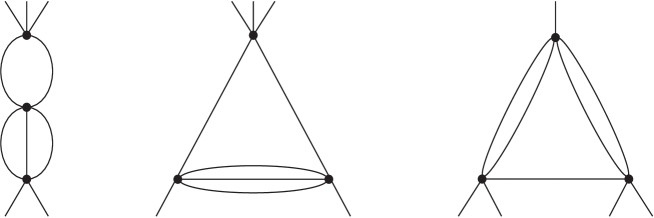
Figure 2: Leading order topologies for $5$-point function in scalar $\phi^{5}$ theory.

Figure 3: Leading order topologies for $7$-point functions in scalar $\phi^{7}$ theory.

3 Results.

Having outlined the computation methodology we now present the results for the various theories. First, for the case of $n$ $=$ $5$ we have

$$\beta^{\phi^{5}}(g) = -~{}3\epsilon g~{}+~{}\frac{1377}{16}\Gamma^{3}\left(\frac{2}{3}\right)g^{3}~{}+~{}O(g^{5})$$

$$\gamma^{\phi^{5}}_{\phi}(g) = -~{}\frac{3}{80}\Gamma^{3}\left(\frac{2}{3}\right)g^{2}~{}+~{}O(g^{4})$$

$$\gamma^{\phi^{5}}_{\cal O}(g) = \frac{63}{80}\Gamma^{3}\left(\frac{2}{3}\right)g^{2}~{}+~{}O(g^{4})~{}.$$ (3.1)

For this and some other cases we will include the anomalous dimension of the mass operator

$${\cal O}~{}=~{}\frac{1}{2}\phi^{2}~{}.$$ (3.2)

Its renormalization is carried out by inserting the operator in a $2$-point function. Also the graphs which contribute are generated by Qgraf but we have not illustrated these graphically. Instead they can be deduced from the vertex topologies as they can be derived from graphs where there are only two internal propagators connecting with an external vertex. Replacing that vertex by the operator ${\cal O}$ gives a contributing topology to the $2$-point function for the operator renormalization. As an application of these renormalization group functions we have evaluated the critical exponent $\sigma$ which was estimated in [15] using functional renormalization group methods. The exponent is defined by the hyperscaling relation

$$\sigma~{}=~{}\frac{(d-2+2\eta)}{(d+2-2\eta)}$$ (3.3)

where $d$ $=$ $\frac{10}{3}$ $-$ $2\epsilon$, $\eta$ $=$ $\gamma^{\phi^{5}}_{\phi}(g_{c})$ and $g_{c}$ is the non-zero critical coupling constant given by the solution of $\beta^{\phi^{5}}(g_{c})$ $=$ $0$. It corresponds to a Wilson-Fisher fixed point. We find

$$\sigma~{}=~{}\frac{1}{4}~{}-~{}\frac{115}{408}\epsilon~{}+~{}O(\epsilon^{2})$$ (3.4)

or

$$\sigma~{}=~{}0.250000~{}-~{}0.281863\epsilon~{}+~{}O(\epsilon^{2})$$ (3.5)

numerically. As has been widely noted since the critical dimension of this theory is close to an integer dimension then the convergence of the $\epsilon$ expansion ought to be faster than say using the $\epsilon$ expansion of $\phi^{4}$ theory to extract exponent estimates in three dimensions. For $n$ $=$ $5$ we find

$$\left.\sigma\right|_{d=3}~{}=~{}0.203023$$ (3.6)

which is in agreement with [17]. The value is not unreasonable for a leading order computation when compared to the value of $0.198$ for $\sigma$ using functional renormalization group methods of [15]. Also we have computed the exponent $1/\nu$ from $\gamma^{\phi^{5}}_{\cal O}(g)$ and note that it agrees with [17].

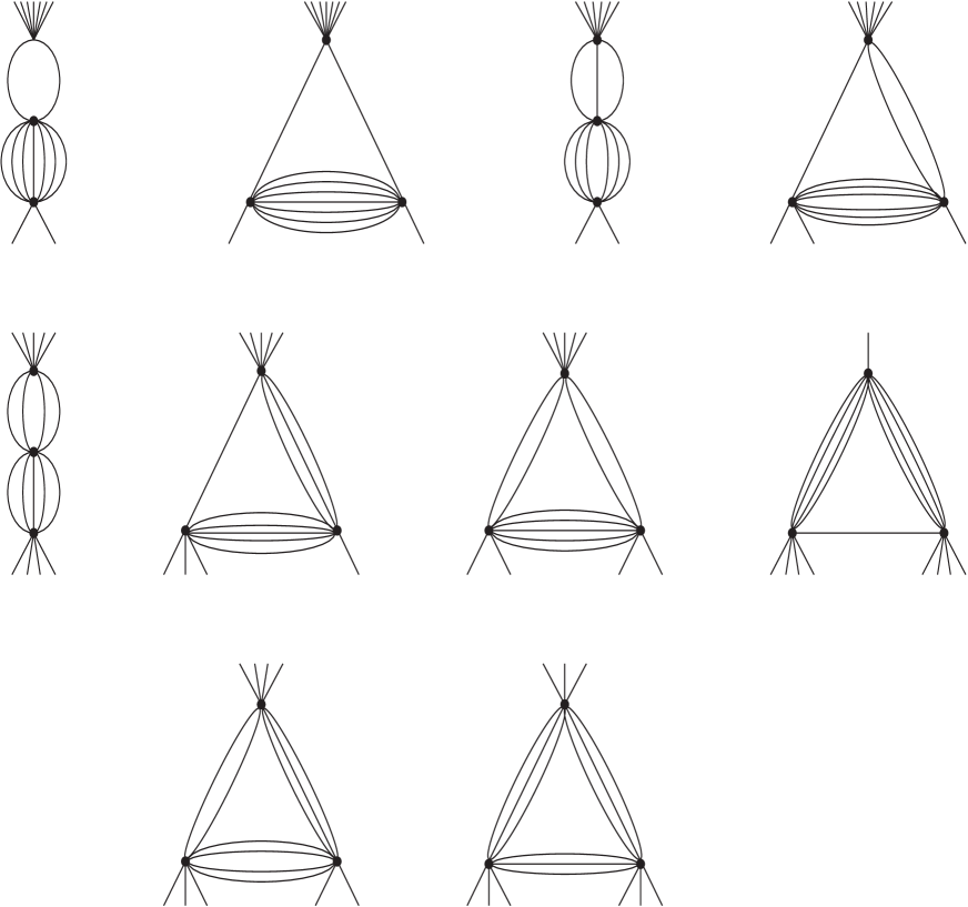
Figure 4: Next to leading order topologies for $9$-point function in $\phi^{9}$ theory.

For the next two odd power potentials we find the following sets of renormalization group functions

$$\beta^{\phi^{7}}(g) = -~{}5\epsilon g~{}+~{}\frac{25}{288}\Gamma^{5}\left(\frac{2}{5}\right)\left[1733+1260\frac{\Gamma^{2}\left(\frac{3}{5}\right)\Gamma\left(\frac{2}{5}\right)}{\Gamma^{2}\left(\frac{4}{5}\right)}\right]g^{3}~{}+~{}O(g^{5})$$

$$\gamma_{\phi}^{\phi^{7}}(g) = -~{}\frac{5}{2016}\Gamma^{5}\left(\frac{2}{5}\right)g^{2}~{}+~{}O(g^{4})$$

$$\gamma_{\cal O}^{\phi^{7}}(g) = \frac{25}{672}\Gamma^{5}\left(\frac{2}{5}\right)g^{2}~{}+~{}O(g^{4})$$ (3.7)

and

$$\beta^{\phi^{9}}(g) = -~{}7\epsilon g$$

$$+~{}\left[-~{}317520\Gamma^{4}\left(\frac{6}{7}\right)\Gamma^{2}\left(\frac{5}{7}\right)\Gamma\left(\frac{2}{7}\right)+364899\Gamma^{3}\left(\frac{6}{7}\right)\Gamma^{2}\left(\frac{4}{7}\right)\Gamma\left(\frac{3}{7}\right)\right.$$

$$\left.~{}~{}~{}~{}+756000\Gamma^{2}\left(\frac{6}{7}\right)\Gamma\left(\frac{5}{7}\right)\Gamma\left(\frac{4}{7}\right)\Gamma^{2}\left(\frac{3}{7}\right)\Gamma\left(\frac{2}{7}\right)+32000\Gamma^{2}\left(\frac{4}{7}\right)\Gamma^{4}\left(\frac{3}{7}\right)\Gamma\left(\frac{2}{7}\right)\right]$$

$$~{}~{}~{}~{}\times\frac{49\Gamma^{7}\left(\frac{2}{7}\right)g^{3}}{172800\Gamma^{3}\left(\frac{6}{7}\right)\Gamma^{2}\left(\frac{4}{7}\right)\Gamma\left(\frac{3}{7}\right)}~{}+~{}O(g^{5})$$

$$\gamma^{\phi^{9}}_{\phi}(g) = -~{}\frac{7}{103680}\Gamma^{7}\left(\frac{2}{7}\right)g^{2}~{}+~{}O(g^{4})$$ (3.8)

where $D_{9}$ $=$ $\frac{18}{7}$. In comparison with $\beta^{\phi^{5}}(g)$ both $\beta$-functions have a new feature in that there are two distinct terms in contrast to the one of the $n$ $=$ $5$ theory. By this we mean two independent combinations of $\Gamma$-functions.

It transpires, however, that this first occurs in the $n$ $=$ $6$ theory since

$$\beta^{\phi^{6}}(g) = -~{}4\epsilon g~{}+~{}\frac{20\pi}{3}g^{2}~{}-~{}\left[225\pi^{2}+2248\right]\frac{\pi^{2}g^{3}}{30}~{}+~{}O(g^{5})$$

$$\gamma^{\phi^{6}}_{\phi}(g) = \frac{\pi^{2}}{45}g^{2}~{}-~{}\frac{4\pi^{3}}{81}g^{3}~{}+~{}O(g^{4})~{}.$$ (3.9)

These were computed in [8, 9] and extended to the next order in [12]. We evaluated them here as a check on our computation method before applying it to the odd power potentials. While there was a mismatch in the one loop terms of the $n$ $=$ $7$ theory it occurs first at two loops for $n$ $=$ $6$. Therefore we expect that the first occurrence of the mismatch for $n$ $=$ $5$ will be at two loops. For $n$ $=$ $8$ the $\beta$-function has a similar structure to $n$ $=$ $6$ since

$$\beta^{\phi^{8}}(g) = -~{}6\epsilon g~{}+~{}\frac{70\pi^{3}\sqrt{3}}{9\Gamma^{3}\left(\frac{2}{3}\right)}g^{2}$$

$$+~{}\left[297675\pi\sqrt{3}\Gamma^{3}\left(\frac{2}{3}\right)-313600\pi^{3}\sqrt{3}-893025\ln 3\,\Gamma^{3}\left(\frac{2}{3}\right)\right.$$

$$~{}~{}~{}~{}~{}\left.-~{}3082536\Gamma^{3}\left(\frac{2}{3}\right)\right]\frac{4\pi^{6}g^{3}}{25515\Gamma^{9}\left(\frac{2}{3}\right)}~{}+~{}O(g^{4})$$

$$\gamma^{\phi^{8}}(g) = \frac{2\pi^{6}}{945\Gamma^{6}\left(\frac{2}{3}\right)}g^{2}~{}-~{}\frac{\pi^{9}\sqrt{3}}{162\Gamma^{9}\left(\frac{2}{3}\right)}g^{3}~{}+~{}O(g^{4})~{}.$$ (3.10)

One of the reasons for highlighting this aspect of the renormalization group function numerology is that the differences reflect the underlying topologies of each vertex function as well as certain properties. For instance one can define a weighted sum for any of the products of $\Gamma$-functions appearing in the $\beta$-functions by summing the products of the $\Gamma$-function arguments with the power. Examining $\beta^{\phi^{9}}(g)$ the respective index of each of the four terms are $3$, $2$, $2$ and $1$ where we count the contribution from a denominator $\Gamma$-function in the sum as negative. For $n$ $=$ $5$ we have $2$ for both terms in the $\beta$-function. For the even dimensional cases the various powers of $\pi$, $\ln 3$ and $\sqrt{3}$ would first have to be re-expressed in terms of $\Gamma$-functions. For the well-studied cases of $n$ $=$ $3$ and $4$ the same aspect of weighting is present. The difference is that the $\Gamma$-functions are already hidden in the corresponding expression as they will have arisen with integer arguments. Although drawing attention to this particular weighting or property of the renormalization group functions in rational dimensions may appear to be a quirk, it is in fact a guide to the expectations of the series of various sums which can appear at higher loop order. For instance the corrections to the $n$ $=$ $6$ theory are known to the next order to that given above, [12]. The various numbers which appear there are new nested sums which are not present even at four loops in $n$ $=$ $3$ and $4$. Instead in the latter the nested sums which arise are the usual Riemann $\zeta$-function at integer argument which lead to more complicated sums at much higher loops. For a variety of articles on this topic see, for instance, [40, 41, 42, 43, 44]. Indeed we now know the coefficients of such new irrationals in the $O(N)$ $\phi^{4}$ $\beta$-function at six and seven loops, [28, 29, 30]. As the appearance of the Riemann $\zeta$-function is as a consequence of the seeding by the hidden $\Gamma$-functions of integer argument, then by the same token we would expect the appearance of new sums in the rational critical dimension theories seeded by combinations of $\Gamma$-functions with rational arguments.

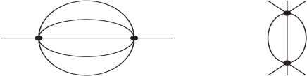
Figure 5: Leading order topologies for $\phi^{6}$.

4 $O(N)$ symmetric theories.

Having concentrated on the basic scalar theories with one field we now turn to the case where the field has an $O(N)$ symmetry. Studies of $O(N)$ symmetric theories in fractional dimensions have been carried out previously in [16] for example. Here our motivation is to extend the renormalization group functions of theories considered in the previous section. One aim is to provide this information ahead of the application of conformal field theory ideas such as those developed in [21] to $O(N)$ symmetric potentials. In [21] conformal methods were used to compute critical exponents from which the renormalization group functions were constructed. A second reason is to highlight a possible connection between various theories with an $O(N)$ symmetry. To appreciate this it is perhaps best to recall a connection which has been widely studied. For instance, $O(N)$ symmetric $\phi^{4}$ theory can be described by the Lagrangian of bare quantities

$$L_{N}^{\phi^{4}}~{}=~{}\frac{1}{2}\partial_{\mu}\phi^{i}_{\mbox{\footnotesize{o}}}\partial^{\mu}\phi^{i}_{\mbox{\footnotesize{o}}}~{}+~{}\frac{g_{\mbox{\footnotesize{o}}}}{2}\sigma_{\mbox{\footnotesize{o}}}\phi^{i}_{\mbox{\footnotesize{o}}}\phi^{i}_{\mbox{\footnotesize{o}}}~{}-~{}\frac{1}{2}\sigma_{\mbox{\footnotesize{o}}}^{2}$$ (4.1)

where $\sigma_{\mbox{\footnotesize{o}}}$ is an auxiliary field here and is not to be confused with the exponent which was introduced briefly earlier and its associated renormalization constant here and elsewhere is

$$\sigma_{\mbox{\footnotesize{o}}}~{}=~{}\sqrt{Z_{\sigma}}\sigma~{}.$$ (4.2)

The elimination of $\sigma_{\mbox{\footnotesize{o}}}$ produces the canonical Lagrangian which is renormalizable in four dimensions. Recently it has been shown, [33, 34], that the ultraviolet completion of $L_{N}^{\phi^{4}}$ is to the Lagrangian $L_{N}^{\phi^{3}}$ where

$$L_{N}^{\phi^{3}}~{}=~{}\frac{1}{2}\partial_{\mu}\phi^{i}_{\mbox{\footnotesize{o}}}\partial^{\mu}\phi^{i}_{\mbox{\footnotesize{o}}}~{}+~{}\frac{1}{2}\partial^{\mu}\sigma_{\mbox{\footnotesize{o}}}\partial_{\mu}\sigma_{\mbox{\footnotesize{o}}}~{}+~{}\frac{g_{1\,\mbox{\footnotesize{o}}}}{2}\sigma_{\mbox{\footnotesize{o}}}\phi^{i}_{\mbox{\footnotesize{o}}}\phi^{i}_{\mbox{\footnotesize{o}}}~{}+~{}\frac{g_{2\,\mbox{\footnotesize{o}}}}{2}\sigma_{\mbox{\footnotesize{o}}}^{3}~{}.$$ (4.3)

In $L_{N}^{\phi^{3}}$ $\sigma$ is not regarded now as an auxiliary field due to the usual kinetic term. Also its cubic self-interaction is required to ensure the Lagrangian is renormalizable in six dimensions. The ultraviolet completion relates to the fact that at the Wilson-Fisher fixed point in dimensions $d$ where $4$ $<$ $d$ $<$ $6$ both theories lie in the same universality class. This is not unrelated to the common interaction between the $\phi^{i}$ and $\sigma$ fields. Indeed one way to establish the universal connection is via the $1/N$ expansion especially in the original formulation given in [45, 46, 47]. In those articles the critical exponents of the universal theory were computed as functions of the spacetime to three terms in the $1/N$ expansion. Expanding the exponents in the neighbourhood of a critical dimension of a theory such as $L_{N}^{\phi^{3}}$ and $L_{N}^{\phi^{4}}$ they are in full agreement with the critical exponents derived from the explicit renormalization group functions of those theories.

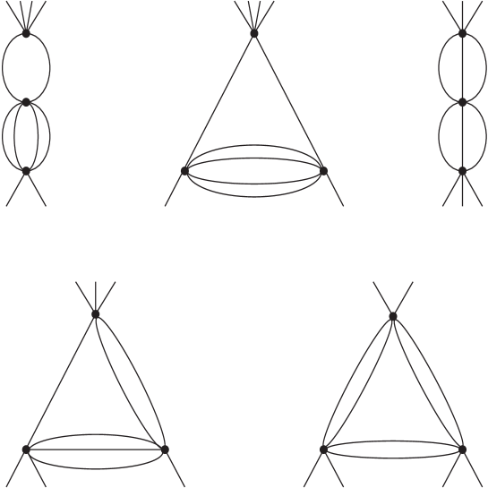
Figure 6: Next to leading order topologies for $6$-point function in $\phi^{6}$ theory.

Having reviewed this well-established connection between $L_{N}^{\phi^{3}}$ and $L_{N}^{\phi^{4}}$ it is worth noting that the latter is in effect a theory with $n$ $=$ $4$ in contrast with the former which has $n$ $=$ $3$. Each is part of the Ising or Lee-Yang class of theories. It turns out that this connectivity extends to some of the theories we consider here. For instance, the next candidate theory to apply this concept to is that recently termed the Blume-Capel class. For instance, the parallel starting point to $L_{N}^{\phi^{4}}$ is $L_{N}^{\phi^{8}}$ where

$$L_{N}^{\phi^{8}}~{}=~{}\frac{1}{2}\partial_{\mu}\phi^{i}_{\mbox{\footnotesize{o}}}\partial^{\mu}\phi^{i}_{\mbox{\footnotesize{o}}}~{}+~{}\frac{g^{2}_{\mbox{\footnotesize{o}}}}{40320}(\phi^{i}_{\mbox{\footnotesize{o}}}\phi^{i}_{\mbox{\footnotesize{o}}})^{4}~{}.$$ (4.4)

The interaction which is clearly in the $n$ $=$ $8$ class can be reformulated with an auxiliary field $\sigma$ via

$$L_{N}^{\phi^{8}}~{}=~{}\frac{1}{2}\partial_{\mu}\phi^{i}_{\mbox{\footnotesize{o}}}\partial^{\mu}\phi^{i}_{\mbox{\footnotesize{o}}}~{}+~{}\frac{g_{\mbox{\footnotesize{o}}}}{24}\sigma_{\mbox{\footnotesize{o}}}(\phi^{i}_{\mbox{\footnotesize{o}}}\phi^{i}_{\mbox{\footnotesize{o}}})^{2}~{}-~{}\frac{35}{2}\sigma_{\mbox{\footnotesize{o}}}^{2}~{}.$$ (4.5)

While the critical dimension is still $\frac{8}{3}$ the core interaction has an $n$ $=$ $5$ structure. Therefore to investigate whether there is a common universality class underlying $L_{N}^{\phi^{8}}$ and an $O(N)$ symmetric $n$ $=$ $5$ theory parallel to the $L_{N}^{\phi^{3}}$ and $L_{N}^{\phi^{4}}$ one the first stage is to construct the corresponding renormalization group functions for $L_{N}^{\phi^{8}}$ and the potentially related one which we will term $L_{N}^{\phi^{5}}$. Based on the commonality of the core interaction in the $\sigma$ field formulation of $L_{N}^{\phi^{3}}$ and $L_{N}^{\phi^{4}}$ we follow the same prescription of building a renormalizable Lagrangian in $D_{5}$ based on the $n$ $=$ $5$ $O(N)$ symmetric interaction of $L_{N}^{\phi^{8}}$. This produces

$$L_{N}^{\phi^{5}} = \frac{1}{2}\partial_{\mu}\phi^{i}_{\mbox{\footnotesize{o}}}\partial^{\mu}\phi^{i}_{\mbox{\footnotesize{o}}}~{}+~{}\frac{1}{2}\partial_{\mu}\sigma_{\mbox{\footnotesize{o}}}\partial^{\mu}\sigma_{\mbox{\footnotesize{o}}}~{}+~{}\frac{g_{1\,\mbox{\footnotesize{o}}}}{24}\sigma_{\mbox{\footnotesize{o}}}(\phi^{i}_{\mbox{\footnotesize{o}}}\phi^{i}_{\mbox{\footnotesize{o}}})^{2}~{}+~{}\frac{g_{2\,\mbox{\footnotesize{o}}}}{12}\sigma^{3}_{\mbox{\footnotesize{o}}}\phi^{i}_{\mbox{\footnotesize{o}}}\phi^{i}_{\mbox{\footnotesize{o}}}~{}+~{}\frac{g_{3\,\mbox{\footnotesize{o}}}}{120}\sigma_{\mbox{\footnotesize{o}}}^{5}$$ (4.6)

which has quintic interactions and a propagating $\sigma$ field. Unlike $L_{N}^{\phi^{3}}$ there is an additional interaction between $\phi^{i}$ and $\sigma$ from renormalizability. While this potential connection will serve as a motivation for constructing the renormalization group functions we will also renormalize the following remaining $O(N)$ symmetric Lagrangians

$$L_{N}^{\phi^{6}} = \frac{1}{2}\partial_{\mu}\phi^{i}_{\mbox{\footnotesize{o}}}\partial^{\mu}\phi^{i}_{\mbox{\footnotesize{o}}}~{}+~{}\frac{g_{\mbox{\footnotesize{o}}}}{720}(\phi^{i}_{\mbox{\footnotesize{o}}}\phi^{i}_{\mbox{\footnotesize{o}}})^{3}$$

$$L_{N}^{\phi^{7}} = \frac{1}{2}\partial_{\mu}\phi^{i}_{\mbox{\footnotesize{o}}}\partial^{\mu}\phi^{i}_{\mbox{\footnotesize{o}}}~{}+~{}\frac{1}{2}\partial_{\mu}\sigma_{\mbox{\footnotesize{o}}}\partial^{\mu}\sigma_{\mbox{\footnotesize{o}}}~{}+~{}\frac{g_{1\,\mbox{\footnotesize{o}}}}{720}\sigma_{\mbox{\footnotesize{o}}}(\phi^{i}_{\mbox{\footnotesize{o}}}\phi^{i}_{\mbox{\footnotesize{o}}})^{3}~{}+~{}\frac{g_{2\,\mbox{\footnotesize{o}}}}{144}\sigma_{\mbox{\footnotesize{o}}}^{3}(\phi^{i}_{\mbox{\footnotesize{o}}}\phi^{i}_{\mbox{\footnotesize{o}}})^{2}$$

$$+~{}\frac{g_{3\,\mbox{\footnotesize{o}}}}{240}\sigma_{\mbox{\footnotesize{o}}}^{5}\phi^{i}_{\mbox{\footnotesize{o}}}\phi^{i}_{\mbox{\footnotesize{o}}}~{}+~{}\frac{g_{4\,\mbox{\footnotesize{o}}}}{5040}\sigma_{\mbox{\footnotesize{o}}}^{7}$$

$$L_{N}^{\phi^{9}} = \frac{1}{2}\partial_{\mu}\phi^{i}_{\mbox{\footnotesize{o}}}\partial^{\mu}\phi^{i}_{\mbox{\footnotesize{o}}}~{}+~{}\frac{1}{2}\partial_{\mu}\sigma_{\mbox{\footnotesize{o}}}\partial^{\mu}\sigma_{\mbox{\footnotesize{o}}}~{}+~{}\frac{g_{1\,\mbox{\footnotesize{o}}}}{40320}\sigma_{\mbox{\footnotesize{o}}}(\phi^{i}_{\mbox{\footnotesize{o}}}\phi^{i}_{\mbox{\footnotesize{o}}})^{4}~{}+~{}\frac{g_{2\,\mbox{\footnotesize{o}}}}{4320}\sigma_{\mbox{\footnotesize{o}}}^{3}(\phi^{i}_{\mbox{\footnotesize{o}}}\phi^{i}_{\mbox{\footnotesize{o}}})^{3}$$ (4.7)

$$+~{}\frac{g_{3\,\mbox{\footnotesize{o}}}}{2880}\sigma_{\mbox{\footnotesize{o}}}^{5}(\phi^{i}_{\mbox{\footnotesize{o}}}\phi^{i}_{\mbox{\footnotesize{o}}})^{2}~{}+~{}\frac{g_{4\,\mbox{\footnotesize{o}}}}{10080}\sigma_{\mbox{\footnotesize{o}}}^{7}\phi^{i}_{\mbox{\footnotesize{o}}}\phi^{i}_{\mbox{\footnotesize{o}}}~{}+~{}\frac{g_{5\,\mbox{\footnotesize{o}}}}{362880}\sigma_{\mbox{\footnotesize{o}}}^{9}~{}.$$

The Lagrangian $L_{N}^{\phi^{6}}$ was studied previously in [12] and is similar in structure to $L_{N}^{\phi^{8}}$. By contrast for odd $n$ there are an increasing number of interactions to ensure renormalizability. Consequently there is a significantly larger number of Feynman graphs to be evaluated. We have given an indication of this for the renormalization of the fields and coupling constants for Lagrangians with an odd value of $n$ in Table $2$.

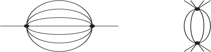
Figure 7: Leading order topologies for $\phi^{8}$.

$n$	$\phi^{i}$	$\sigma$	$g_{1}$	$g_{2}$	$g_{3}$	$g_{4}$	$g_{5}$
$5$	$2$	$3$	$135$	$137$	$155$	—	—
$7$	$3$	$4$	$2644$	$2688$	$2692$	$2912$	—
$9$	$4$	$5$	$42607$	$43149$	$43147$	$43241$	$42607$

Table 2. Number of graphs computed for the renormalization of the field and each coupling constant for $O(N)$ symmetric theories for odd $n$.

In light of this we note that the Lagrangian for higher order interaction equivalences is straightforward to write down. The Lagrangian $L_{N}^{\phi^{4r}}$ should have connection with $L_{N}^{\phi^{2r+1}}$ for integer $r$ where

$$L_{N}^{\phi^{4r}}~{}=~{}\frac{1}{2}\partial_{\mu}\phi^{i}_{\mbox{\footnotesize{o}}}\partial^{\mu}\phi^{i}_{\mbox{\footnotesize{o}}}~{}+~{}\frac{g_{\mbox{\footnotesize{o}}}}{(4r)!}(\phi^{i}_{\mbox{\footnotesize{o}}}\phi^{i}_{\mbox{\footnotesize{o}}})^{2r}$$ (4.8)

and $L_{N}^{\phi^{2r+1}}$ has the core interaction $\sigma(\phi^{i}\phi^{i})^{r}$ leading to

$$L_{N}^{\phi^{2r+1}}~{}=~{}\frac{1}{2}\partial_{\mu}\phi^{i}_{\mbox{\footnotesize{o}}}\partial^{\mu}\phi^{i}_{\mbox{\footnotesize{o}}}~{}+~{}\frac{1}{2}\partial_{\mu}\sigma_{\mbox{\footnotesize{o}}}\partial^{\mu}\sigma_{\mbox{\footnotesize{o}}}~{}+~{}\sum_{p=0}^{r}g_{p+1\,\mbox{\footnotesize{o}}}\sigma_{\mbox{\footnotesize{o}}}^{2p+1}(\phi^{i}_{\mbox{\footnotesize{o}}}\phi^{i}_{\mbox{\footnotesize{o}}})^{r-p}~{}.$$ (4.9)

In making this connection with various odd and even potentials it is straightforward to write down the Lagrangian of the limiting critical dimension. To see the connection between $L_{N}^{\phi^{2r+1}}$ and $L_{N}^{\phi^{4r}}$ via the same $n$-point vertex we introduce the auxiliary field $\sigma$ as in (4.1) and (4.5). In the former there is a theory with a lower critical dimension which is in the same universality class as $L_{N}^{\phi^{4}}$ and is the nonlinear $\sigma$ model (nlsm) which has a Lagrangian and can be written as

$$L_{N}^{\mbox{\footnotesize{nlsm}}}~{}=~{}\frac{1}{2}\partial_{\mu}\phi^{i}_{\mbox{\footnotesize{o}}}\partial^{\mu}\phi^{i}_{\mbox{\footnotesize{o}}}~{}+~{}\frac{g_{\mbox{\footnotesize{o}}}}{2}\sigma_{\mbox{\footnotesize{o}}}\phi^{i}_{\mbox{\footnotesize{o}}}\phi^{i}_{\mbox{\footnotesize{o}}}~{}-~{}\frac{1}{2}\sigma_{\mbox{\footnotesize{o}}}~{}.$$ (4.10)

Here $\sigma$ is regarded as a Lagrange multiplier field and its role is to constrain the fields $\phi^{i}$ to lie on a sphere. Also the critical dimension of (4.10) is $2$ and in this dimension $\sigma$ has canonical dimension $2$ whereas the $\phi^{i}$ field is dimensionless. However with parallel Lagrangians based on higher order potentials also available one can write down similar Lagrangians which are linear in $\sigma$ and which have critical dimension $2$. This can be generalized to the Lagrangian

$$L_{N}^{\phi^{\infty}}~{}=~{}\frac{1}{2}\partial_{\mu}\phi^{i}_{\mbox{\footnotesize{o}}}\partial^{\mu}\phi^{i}_{\mbox{\footnotesize{o}}}~{}+~{}\frac{1}{2}\sum_{n=0}^{\infty}g_{n\,\mbox{\footnotesize{o}}}\sigma_{\mbox{\footnotesize{o}}}(\phi^{i}_{\mbox{\footnotesize{o}}}\phi^{i}_{\mbox{\footnotesize{o}}})^{n}$$ (4.11)

where all possible interactions are available and has $D_{\infty}$ $=$ $2$. One can regard (4.11) as the theory corresponding to (2.5) in the $n$ $\to$ $\infty$ limit. Equally it could be viewed as the base two dimensional Lagrangian from which each of the $D_{n}$ $>$ $2$ theories we have considered here, as well as others, are related to through their corresponding Wilson-Fisher fixed point. In some sense it is the two dimensional universal Lagrangian of all the univerality classes of scalar $O(N)$ theories. The connection of each interaction relative to its critical dimension and two dimensions is apparent if one considers the structure of the leading order graph contributing to the $2$-point function renormalization such as those illustrated in Figures 1, 5 and 7 for example. If we denote such a graph with $L$ loops by $\Gamma_{(2),L}$ then its evaluation is

$$\Gamma_{(2),L}~{}=~{}\frac{\Gamma^{L+1}\left(\frac{d}{2}-1\right)\Gamma\left(L+1-\frac{d}{2}L\right)}{\Gamma\left(\frac{d}{2}(L+1)-(L+1)\right)}$$ (4.12)

which corresponds to a $\phi^{L+2}$ potential. This function diverges when the argument of either numerator $\Gamma$-functions is zero or negative. Clearly this will occur for all $L$ $\geq$ $1$ when $d$ $=$ $2$ due to $\Gamma\left(\frac{d}{2}-1\right)$. For lower values of $d$ this is not meaningful. By contrast the other numerator $\Gamma$-function diverges for certain dimensions but this depends on $L$ and hence the specific potential. More crucially for (4.11) the critical dimensions $D_{n}$ emerge for each potential when this $\Gamma$-function has argument $(-1)$. Therefore at the initial renormalization stage the Lagrangian (4.11) reflects the dimensional connection. Of course there are other singularities in this specific $\Gamma$-function when the argument is any other negative integer or zero but these do not correspond to the critical dimensions of any of the Lagrangians we consider here. Instead several may correspond to their higher dimensional ultraviolet completions.

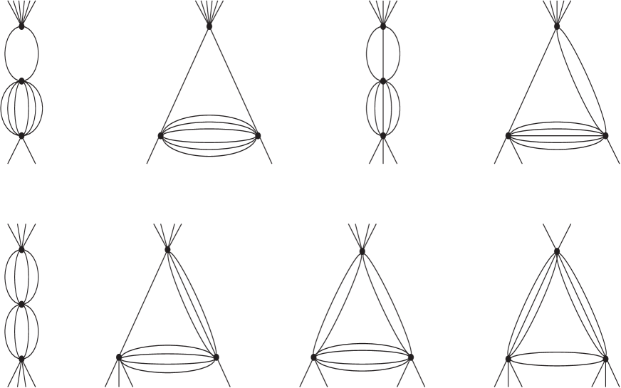
Figure 8: Next to leading order topologies for $8$-point function in $\phi^{8}$ theory.

We now proceed to the task of recording the results. First, for the potential connection between $L_{N}^{\phi^{5}}$ and $L_{N}^{\phi^{8}}$ we have

$$\gamma_{\phi}^{\phi^{5}}(g_{i}) = -~{}\left[Ng_{1}^{2}+2g_{1}^{2}+3g_{2}^{2}\right]\frac{\Gamma^{3}\left(\frac{2}{3}\right)}{20}~{}+~{}O(g_{i}^{3})$$

$$\gamma_{\sigma}^{\phi^{5}}(g_{i}) = -~{}\left[N^{2}g_{1}^{2}+2Ng_{1}^{2}+18Ng_{2}^{2}+3g_{3}^{2}\right]\frac{\Gamma^{3}\left(\frac{2}{3}\right)}{80}~{}+~{}O(g_{i}^{3})$$

$$\beta_{1}^{\phi^{5}}(g_{i}) = -~{}3\epsilon g_{1}$$

$$+~{}\left[59N^{2}g_{1}^{3}+2182Ng_{1}^{3}+9648g_{1}^{3}+1440Ng_{1}^{2}g_{2}+15840g_{1}^{2}g_{2}+1062Ng_{1}g_{2}^{2}\right.$$

$$\left.~{}~{}~{}~{}+12912g_{1}g_{2}^{2}-480g_{1}g_{2}g_{3}-3g_{1}g_{3}^{2}+10800g_{2}^{3}+1620g_{2}^{2}g_{3}\right]\frac{\Gamma^{3}\left(\frac{2}{3}\right)}{80}~{}+~{}O(g_{i}^{5})$$

$$\beta_{2}^{\phi^{5}}(g_{i}) = -~{}3\epsilon g_{2}$$

$$+~{}\left[80N^{2}g_{1}^{3}+1040Ng_{1}^{3}+1760g_{1}^{3}+177N^{2}g_{1}^{2}g_{2}+2506Ng_{1}^{2}g_{2}+4304g_{1}^{2}g_{2}\right.$$

$$\left.~{}~{}~{}~{}-40Ng_{1}^{2}g_{3}-80g_{1}^{2}g_{3}+5400Ng_{1}g_{2}^{2}+10800g_{1}g_{2}^{2}+540Ng_{1}g_{2}g_{3}\right.$$

$$\left.~{}~{}~{}~{}+1080g_{1}g_{2}g_{3}+486Ng_{2}^{3}+17136g_{2}^{3}+8640g_{2}^{2}g_{3}+1251g_{2}g_{3}^{2}\right]\frac{\Gamma^{3}\left(\frac{2}{3}\right)}{80}~{}+~{}O(g_{i}^{5})$$

$$\beta_{3}^{\phi^{5}}(g_{i}) = -~{}3\epsilon g_{3}$$ (4.13)

$$+~{}\left[-~{}80N^{2}g_{1}^{2}g_{2}-160Ng_{1}^{2}g_{2}-N^{2}g_{1}^{2}g_{3}-2Ng_{1}^{2}g_{3}+540N^{2}g_{1}g_{2}^{2}+1080Ng_{1}g_{2}^{2}\right.$$

$$\left.~{}~{}~{}~{}+5760Ng_{2}^{3}+2502Ng_{2}^{2}g_{3}+1377g_{3}^{3}\right]\frac{\Gamma^{3}\left(\frac{2}{3}\right)}{16}~{}+~{}O(g_{i}^{5})$$

and

$$\gamma_{\phi}^{\phi^{8}}(g) = \frac{2\pi^{6}}{99225\Gamma^{6}\left(\frac{2}{3}\right)}[N+2][N+4][N+6]g^{2}$$

$$-~{}\frac{\pi^{9}\sqrt{3}}{20837250\Gamma^{9}\left(\frac{2}{3}\right)}[N+2][N+4][N+6][3N^{2}+150N+1072]g^{3}~{}+~{}O(g^{4})$$

$$\gamma_{\cal O}^{\phi^{8}}(g) = \frac{26\pi^{6}}{99225\Gamma^{6}\left(\frac{2}{3}\right)}[N+2][N+4][N+6]g^{2}~{}+~{}O(g^{3})$$

$$\beta^{\phi^{8}}(g) = -~{}6\epsilon g~{}+~{}\frac{2\pi^{3}\sqrt{3}}{\Gamma^{3}\left(\frac{2}{3}\right)}\left[\frac{1072}{315}+\frac{10}{21}N+\frac{1}{105}N^{2}\right]g^{2}$$ (4.14)

$$+\left[-~{}\frac{\pi^{6}}{\Gamma^{6}\left(\frac{2}{3}\right)}\left[\frac{164480}{441}+\frac{74464}{735}N+\frac{4576}{525}N^{2}+\frac{184}{735}N^{3}+\frac{8}{3675}N^{4}\right]\right.$$

$$\left.~{}~{}~{}~{}-\frac{\pi^{6}\ln{3}}{\Gamma^{6}\left(\frac{2}{3}\right)}\left[\frac{26496}{245}+\frac{15392}{525}N+\frac{9056}{3675}N^{2}+\frac{256}{3675}N^{3}+\frac{4}{3675}N^{4}\right]\right.$$

$$\left.~{}~{}~{}~{}-\frac{\pi^{9}\sqrt{3}}{\Gamma^{9}\left(\frac{2}{3}\right)}\left[\frac{11558912}{297675}+\frac{1712128}{178605}N+\frac{217088}{297675}N^{2}+\frac{1024}{59535}N^{3}\right]\right.$$

$$\left.~{}~{}~{}~{}+\frac{\pi^{7}\sqrt{3}}{\Gamma^{6}\left(\frac{2}{3}\right)}\left[\frac{8832}{245}+\frac{15392}{1575}N+\frac{9056}{11025}N^{2}+\frac{256}{11025}N^{3}+\frac{4}{11025}N^{4}\right]\right]g^{3}$$

$$+~{}O(g^{4})$$

where the order symbol for the multi-coupling theories denotes all possible combinations of the couplings. We have also recorded the mass operator dimension in passing. While the $\beta$-function in (4.14) is not asymptotically free there is a Banks-Zaks fixed point, [48] for all $N$. Given the proximity of the critical dimension of $\phi^{8}$ theory to two dimensions it ought to be possible to use the $\epsilon$-expansion to estimate the wave function critical exponent in that lower spacetime. For instance, when $N$ $=$ $1$ it is known, [13], that $\phi^{8}$ theory corresponds to the unitary, conformal, minimal model with $c$ $=$ $\frac{4}{5}$. However, it was shown in [13] that a sizeable number of terms of the $\epsilon$-expansion would be required to have approximate agreement.

For the remaining two theories we are concentrating on we have

$$\gamma_{\phi}^{\phi^{7}}(g_{i}) = -~{}\left[\frac{5}{336}g_{3}^{2}+\frac{25}{756}g_{2}^{2}+\frac{1}{126}g_{1}^{2}+\frac{25}{1512}Ng_{2}^{2}+\frac{1}{168}Ng_{1}^{2}+\frac{1}{1008}N^{2}g_{1}^{2}\right]\Gamma^{5}\left(\frac{2}{5}\right)$$

$$+~{}O(g_{i}^{3})$$

$$\gamma_{\sigma}^{\phi^{7}}(g_{i}) = -~{}\left[\frac{5}{2016}g_{4}^{2}+\frac{25}{672}Ng_{3}^{2}+\frac{25}{1008}Ng_{2}^{2}+\frac{1}{756}Ng_{1}^{2}+\frac{25}{2016}N^{2}g_{2}^{2}+\frac{1}{1008}N^{2}g_{1}^{2}\right.$$

$$\left.~{}~{}~{}~{}+\frac{1}{6048}N^{3}g_{1}^{2}\right]\Gamma^{5}\left(\frac{2}{5}\right)~{}+~{}O(g_{i}^{3})$$

$$\beta_{1}^{\phi^{7}}(g_{i}) = -~{}5\epsilon g_{1}$$

$$+\left[-\frac{625}{48}g_{2}g_{3}g_{4}+\frac{9875}{24}g_{2}g_{3}^{2}+\frac{625}{18}g_{2}^{2}g_{4}+\frac{8125}{12}g_{2}^{2}g_{3}+\frac{18625}{18}g_{2}^{3}-\frac{5}{2016}g_{1}g_{4}^{2}\right.$$

$$\left.~{}~{}~{}~{}-\frac{5}{12}g_{1}g_{3}g_{4}-\frac{460}{7}g_{1}g_{3}^{2}+\frac{1225}{9}g_{1}g_{2}g_{3}+\frac{246275}{189}g_{1}g_{2}^{2}+515g_{1}^{2}g_{2}+\frac{18932}{63}g_{1}^{3}\right.$$

$$\left.~{}~{}~{}~{}-\frac{625}{24}Ng_{2}^{2}g_{3}+\frac{3625}{36}Ng_{2}^{3}-\frac{1775}{672}Ng_{1}g_{3}^{2}+\frac{1225}{18}Ng_{1}g_{2}g_{3}+\frac{471775}{3024}Ng_{1}g_{2}^{2}\right.$$

$$\left.~{}~{}~{}~{}+\frac{395}{4}Ng_{1}^{2}g_{2}+\frac{8165}{108}Ng_{1}^{3}-\frac{5275}{2016}N^{2}g_{1}g_{2}^{2}+\frac{65}{8}N^{2}g_{1}^{2}g_{2}+\frac{647}{144}N^{2}g_{1}^{3}\right.$$

$$\left.~{}~{}~{}~{}-\frac{211}{6048}N^{3}g_{1}^{3}\right]\Gamma^{5}\left(\frac{2}{5}\right)$$

$$+\left[\frac{375}{8}g_{3}^{3}+\frac{125}{g}_{2}g_{3}^{2}+\frac{1750}{3}g_{2}^{2}g_{3}+875g_{2}^{3}+\frac{350}{3}g_{1}g_{2}g_{3}+\frac{12875}{18}g_{1}g_{2}^{2}+470g_{1}^{2}g_{2}\right.$$

$$\left.~{}~{}~{}~{}+\frac{632}{3}g_{1}^{3}+\frac{625}{24}Ng_{2}^{2}g_{3}+\frac{125}{2}Ng_{2}^{3}+\frac{25}{3}Ng_{1}g_{2}g_{3}+\frac{1325}{12}Ng_{1}g_{2}^{2}+90Ng_{1}^{2}g_{2}\right.$$

$$\left.~{}~{}~{}~{}+\frac{311}{6}Ng_{1}^{3}+\frac{175}{72}N^{2}g_{1}g_{2}^{2}+\frac{5}{2}N^{2}g_{1}^{2}g_{2}+\frac{37}{12}N^{2}g_{1}^{3}+\frac{1}{24}N^{3}g_{1}^{3}\right]\frac{\Gamma^{6}\left(\frac{2}{5}\right)\Gamma^{2}\left(\frac{3}{5}\right)}{\Gamma^{2}\left(\frac{4}{5}\right)}$$

$$+~{}O(g_{i}^{5})$$

$$\beta_{2}^{\phi^{7}}(g_{i}) = -~{}5\epsilon g_{2}$$

$$+\left[\frac{375}{8}g_{3}^{2}g_{4}+\frac{2725}{12}g_{3}^{3}-\frac{1895}{672}g_{2}g_{4}^{2}+\frac{245}{6}g_{2}g_{3}g_{4}+\frac{18245}{28}g_{2}g_{3}^{2}+\frac{3475}{3}g_{2}^{2}g_{3}\right.$$

$$\left.~{}~{}~{}~{}+\frac{492725}{567}g_{2}^{3}-\frac{25}{12}g_{1}g_{3}g_{4}+\frac{395}{6}g_{1}g_{3}^{2}+\frac{100}{9}g_{1}g_{2}g_{4}+\frac{650}{3}g_{1}g_{2}g_{3}+\frac{1490}{3}g_{1}g_{2}^{2}\right.$$

$$\left.~{}~{}~{}~{}+\frac{98}{9}g_{1}^{2}g_{3}+\frac{39404}{189}g_{1}^{2}g_{2}+\frac{412}{15}g_{1}^{3}+\frac{47525}{672}Ng_{2}g_{3}^{2}+\frac{425}{3}Ng_{2}^{2}g_{3}+\frac{1869475}{9072}Ng_{2}^{3}\right.$$

$$\left.~{}~{}~{}~{}-\frac{25}{48}Ng_{1}g_{3}g_{4}+\frac{395}{24}Ng_{1}g_{3}^{2}+\frac{25}{9}Ng_{1}g_{2}g_{4}+\frac{275}{6}Ng_{1}g_{2}g_{3}+\frac{345}{2}Ng_{1}g_{2}^{2}\right.$$

$$\left.~{}~{}~{}~{}+\frac{49}{6}Ng_{1}^{2}g_{3}+\frac{925}{12}Ng_{1}^{2}g_{2}+\frac{182}{15}Ng_{1}^{3}+\frac{10825}{672}N^{2}g_{2}^{3}-\frac{25}{12}N^{2}g_{1}g_{2}g_{3}\right.$$

$$\left.~{}~{}~{}~{}+\frac{145}{12}N^{2}g_{1}g_{2}^{2}+\frac{49}{36}N^{2}g_{1}^{2}g_{3}+\frac{2515}{432}N^{2}g_{1}^{2}g_{2}+\frac{7}{4}N^{2}g_{1}^{3}-\frac{211}{2016}N^{3}g_{1}^{2}g_{2}\right.$$

$$\left.~{}~{}~{}~{}+\frac{13}{120}N^{3}g_{1}^{3}\right]\Gamma^{5}\left(\frac{2}{5}\right)$$

$$+\left[\frac{175}{8}g_{3}^{2}g_{4}+\frac{375}{2}g_{3}^{3}+25g_{2}g_{3}g_{4}+\frac{3025}{6}g_{2}g_{3}^{2}+25g_{2}^{2}g_{4}+775g_{2}^{2}g_{3}+\frac{32975}{54}g_{2}^{3}\right.$$

$$\left.~{}~{}~{}~{}+20g_{1}g_{3}^{2}+\frac{560}{3}g_{1}g_{2}g_{3}+420g_{1}g_{2}^{2}+\frac{28}{3}g_{1}^{2}g_{3}+\frac{1030}{9}g_{1}^{2}g_{2}+\frac{376}{15}g_{1}^{3}+\frac{325}{12}Ng_{2}g_{3}^{2}\right.$$

$$\left.~{}~{}~{}~{}+\frac{25}{8}Ng_{2}^{2}g_{4}+125Ng_{2}^{2}g_{3}+\frac{5275}{36}Ng_{2}^{3}+5Ng_{1}g_{3}^{2}+55Ng_{1}g_{2}g_{3}+135Ng_{1}g_{2}^{2}\right.$$

$$\left.~{}~{}~{}~{}+3Ng_{1}^{2}g_{3}+\frac{833}{18}Ng_{1}^{2}g_{2}+\frac{166}{15}Ng_{1}^{3}+\frac{475}{216}N^{2}g_{2}^{3}+\frac{25}{12}N^{2}g_{1}g_{2}g_{3}+\frac{15}{2}N^{2}g_{1}g_{2}^{2}\right.$$

$$\left.~{}~{}~{}~{}+\frac{1}{6}N^{2}g_{1}^{2}g_{3}+\frac{173}{36}N^{2}g_{1}^{2}g_{2}+\frac{4}{3}N^{2}g_{1}^{3}+\frac{7}{72}N^{3}g_{1}^{2}g_{2}+\frac{1}{30}N^{3}g_{1}^{3}\right]\frac{\Gamma^{6}\left(\frac{2}{5}\right)\Gamma^{2}\left(\frac{3}{5}\right)}{\Gamma^{2}\left(\frac{4}{5}\right)}$$

$$+~{}O(g_{i}^{5})$$

$$\beta_{3}^{\phi^{7}}(g_{i}) = -~{}5\epsilon g_{3}$$

$$+\left[\frac{25775}{672}g_{3}g_{4}^{2}+\frac{4975}{24}g_{3}^{2}g_{4}+\frac{21775}{28}g_{3}^{3}+\frac{625}{6}g_{2}g_{3}g_{4}+\frac{13625}{18}g_{2}g_{3}^{2}+\frac{1225}{54}g_{2}^{2}g_{4}\right.$$

$$\left.~{}~{}~{}~{}+\frac{91225}{126}g_{2}^{2}g_{3}+\frac{34750}{81}g_{2}^{3}-\frac{125}{54}g_{1}g_{2}g_{4}+\frac{3950}{27}g_{1}g_{2}g_{3}+\frac{3250}{27}g_{1}g_{2}^{2}-\frac{1}{27}g_{1}^{2}g_{4}\right.$$

$$\left.~{}~{}~{}~{}-\frac{736}{63}g_{1}^{2}g_{3}+\frac{980}{81}g_{1}^{2}g_{2}+\frac{81875}{2016}Ng_{3}^{3}+\frac{625}{12}Ng_{2}g_{3}g_{4}+\frac{13625}{36}Ng_{2}g_{3}^{2}\right.$$

$$\left.~{}~{}~{}~{}+\frac{1225}{108}Ng_{2}^{2}g_{4}+\frac{1332325}{3024}Ng_{2}^{2}g_{3}+\frac{21625}{81}Ng_{2}^{3}-\frac{125}{72}Ng_{1}g_{2}g_{4}+\frac{1975}{18}Ng_{1}g_{2}g_{3}\right.$$

$$\left.~{}~{}~{}~{}+\frac{4625}{54}Ng_{1}g_{2}^{2}-\frac{1}{36}Ng_{1}^{2}g_{4}-\frac{997}{108}Ng_{1}^{2}g_{3}+\frac{1225}{81}Ng_{1}^{2}g_{2}+\frac{237625}{6048}N^{2}g_{2}^{2}g_{3}\right.$$

$$\left.~{}~{}~{}~{}+\frac{2125}{81}N^{2}g_{2}^{3}-\frac{125}{432}N^{2}g_{1}g_{2}g_{4}+\frac{1975}{108}N^{2}g_{1}g_{2}g_{3}+\frac{625}{54}N^{2}g_{1}g_{2}^{2}-\frac{1}{216}N^{2}g_{1}^{2}g_{4}\right.$$

$$\left.~{}~{}~{}~{}-\frac{29}{16}N^{2}g_{1}^{2}g_{3}+\frac{490}{81}N^{2}g_{1}^{2}g_{2}-\frac{125}{216}N^{3}g_{1}g_{2}^{2}-\frac{355}{6048}N^{3}g_{1}^{2}g_{3}\right.$$

$$\left.~{}~{}~{}~{}+\frac{245}{324}N^{3}g_{1}^{2}g_{2}\right]\Gamma^{5}\left(\frac{2}{5}\right)$$

$$+\left[\frac{625}{24}g_{3}g_{4}^{2}+\frac{375}{2}g_{3}^{2}g_{4}+\frac{1375}{3}g_{3}^{3}+\frac{875}{18}g_{2}g_{3}g_{4}+625g_{2}g_{3}^{2}+\frac{125}{9}g_{2}^{2}g_{4}+\frac{15125}{27}g_{2}^{2}g_{3}\right.$$

$$\left.~{}~{}~{}~{}+\frac{7750}{27}g_{2}^{3}+25g_{1}g_{3}^{2}+\frac{400}{9}g_{1}g_{2}g_{3}+\frac{2800}{27}g_{1}g_{2}^{2}+\frac{280}{27}g_{1}^{2}g_{2}+\frac{1375}{24}Ng_{3}^{3}\right.$$

$$\left.~{}~{}~{}~{}+\frac{875}{36}Ng_{2}g_{3}g_{4}+\frac{625}{2}Ng_{2}g_{3}^{2}+\frac{125}{18}Ng_{2}^{2}g_{4}+\frac{8375}{27}Ng_{2}^{2}g_{3}+\frac{5125}{27}Ng_{2}^{3}\right.$$

$$\left.~{}~{}~{}~{}+\frac{75}{4}Ng_{1}g_{3}^{2}+\frac{100}{3}Ng_{1}g_{2}g_{3}+\frac{2225}{27}Ng_{1}g_{2}^{2}+\frac{230}{27}Ng_{1}^{2}g_{2}+\frac{1625}{108}N^{2}g_{2}^{2}g_{3}\right.$$

$$\left.~{}~{}~{}~{}+\frac{625}{27}N^{2}g_{2}^{3}+\frac{25}{8}N^{2}g_{1}g_{3}^{2}+\frac{50}{9}N^{2}g_{1}g_{2}g_{3}+\frac{1775}{108}N^{2}g_{1}g_{2}^{2}+\frac{50}{27}N^{2}g_{1}^{2}g_{2}\right.$$

$$\left.~{}~{}~{}~{}+\frac{125}{216}N^{3}g_{1}g_{2}^{2}+\frac{5}{54}N^{3}g_{1}^{2}g_{2}\right]\frac{\Gamma^{6}\left(\frac{2}{5}\right)\Gamma^{2}\left(\frac{3}{5}\right)}{\Gamma^{2}\left(\frac{4}{5}\right)}~{}+~{}O(g_{i}^{5})$$

$$\beta_{4}^{\phi^{7}}(g_{i}) = -~{}5\epsilon g_{4}$$ (4.15)

$$+\left[\frac{43325}{288}g_{4}^{3}+\frac{25775}{32}Ng_{3}^{2}g_{4}+\frac{34825}{24}Ng_{3}^{3}+\frac{4375}{4}Ng_{2}g_{3}^{2}-\frac{9475}{144}Ng_{2}^{2}g_{4}\right.$$

$$\left.~{}~{}~{}~{}+\frac{8575}{18}Ng_{2}^{2}g_{3}-\frac{875}{18}Ng_{1}g_{2}g_{3}+\frac{3500}{27}Ng_{1}g_{2}^{2}-\frac{1}{108}Ng_{1}^{2}g_{4}-\frac{7}{9}Ng_{1}^{2}g_{3}\right.$$

$$\left.~{}~{}~{}~{}+\frac{4375}{8}N^{2}g_{2}g_{3}^{2}-\frac{9475}{288}N^{2}g_{2}^{2}g_{4}+\frac{8575}{36}N^{2}g_{2}^{2}g_{3}-\frac{875}{24}N^{2}g_{1}g_{2}g_{3}+\frac{875}{9}N^{2}g_{1}g_{2}^{2}\right.$$

$$\left.~{}~{}~{}~{}-\frac{1}{144}N^{2}g_{1}^{2}g_{4}-\frac{7}{12}N^{2}g_{1}^{2}g_{3}-\frac{875}{144}N^{3}g_{1}g_{2}g_{3}+\frac{875}{54}N^{3}g_{1}g_{2}^{2}-\frac{1}{864}N^{3}g_{1}^{2}g_{4}\right.$$

$$\left.~{}~{}~{}~{}-\frac{7}{72}N^{3}g_{1}^{2}g_{3}\right]\Gamma^{5}\left(\frac{2}{5}\right)$$

$$+\left[\frac{875}{8}g_{4}^{3}+\frac{4375}{8}Ng_{3}^{2}g_{4}+\frac{2625}{2}Ng_{3}^{3}+\frac{6125}{12}Ng_{2}g_{3}^{2}+\frac{875}{3}Ng_{2}^{2}g_{3}+\frac{1750}{9}Ng_{2}^{3}\right.$$

$$\left.~{}~{}~{}~{}+\frac{6125}{24}N^{2}g_{2}g_{3}^{2}+\frac{875}{6}N^{2}g_{2}^{2}g_{3}+\frac{4375}{36}N^{2}g_{2}^{3}+\frac{875}{72}N^{3}g_{2}^{3}\right]\frac{\Gamma^{6}\left(\frac{2}{5}\right)\Gamma^{2}\left(\frac{3}{5}\right)}{\Gamma^{2}\left(\frac{4}{5}\right)}$$

$$+~{}O(g_{i}^{5})$$

for $L_{N}^{\phi^{7}}$. For $L_{N}^{\phi^{9}}$ the anomalous dimensions are

$$\gamma_{\phi}^{\phi^{9}}(g_{i}) = -~{}\left[N^{3}g_{1}^{2}+12N^{2}g_{1}^{2}+44Ng_{1}^{2}+48g_{1}^{2}+49N^{2}g_{2}^{2}+294Ng_{2}^{2}+392g_{2}^{2}\right.$$

$$\left.~{}~{}~{}~{}+245Ng_{3}^{2}+490g_{3}^{2}+105g_{4}^{2}\right]\frac{\Gamma^{7}\left(\frac{2}{7}\right)}{194400}~{}+~{}O(g_{i}^{3})$$

$$\gamma_{\sigma}^{\phi^{9}}(g_{i}) = -~{}\left[N^{4}g_{1}^{2}+12N^{3}g_{1}^{2}+44N^{2}g_{1}^{2}+48Ng_{1}^{2}+196N^{3}g_{2}^{2}+1176N^{2}g_{2}^{2}+1568Ng_{2}^{2}\right.$$ (4.16)

$$\left.~{}~{}~{}~{}+2450N^{2}g_{3}^{2}+4900Ng_{3}^{2}+2940Ng_{4}^{2}+105g_{5}^{2}\right]\frac{\Gamma^{7}\left(\frac{2}{7}\right)}{1555200}~{}+~{}O(g_{i}^{3})~{}.$$

As there are five couplings for $L_{N}^{\phi^{9}}$ we record only one $\beta$-function explicitly which will suffice for discussion purposes. The remaining $\beta$-functions together with the renormalization group functions for this and all the other Lagrangians are given in the attached data file. We have

$$\beta_{1}^{\phi^{9}}(g_{i}) = -~{}7\epsilon g_{1}$$ (4.17)

$$+~{}\left[\frac{12005}{576}g_{3}^{2}g_{5}+\frac{12005}{27}g_{3}^{2}g_{4}-\frac{2401}{5400}g_{2}g_{4}g_{5}-\frac{81977}{900}g_{2}g_{4}^{2}-\frac{2401}{270}g_{2}g_{3}g_{5}\right.$$

$$\left.~{}~{}~{}~{}+\frac{602651}{1350}g_{2}g_{3}g_{4}+\frac{2020613}{810}g_{2}g_{3}^{2}+\frac{33614}{135}g_{2}^{2}g_{4}+\frac{1745527}{675}g_{2}^{2}g_{3}+\frac{6269354}{3375}g_{2}^{3}\right.$$

$$\left.~{}~{}~{}~{}-\frac{7}{11520}g_{1}g_{5}^{2}-\frac{7}{450}g_{1}g_{4}g_{5}-\frac{1568}{675}g_{1}g_{4}^{2}-\frac{37877}{675}g_{1}g_{3}g_{4}+\frac{900473}{8100}g_{1}g_{3}^{2}\right.$$

$$\left.~{}~{}~{}~{}+\frac{1138172}{2025}g_{1}g_{2}g_{3}+\frac{7829612}{3375}g_{1}g_{2}^{2}+\frac{174412}{375}g_{1}^{2}g_{2}+\frac{933413}{3375}g_{1}^{3}\right.$$

$$\left.~{}~{}~{}~{}+\frac{103243}{2160}Ng_{2}g_{3}g_{4}+\frac{263081}{1620}Ng_{2}g_{3}^{2}-\frac{2401}{540}Ng_{2}^{2}g_{4}+\frac{247303}{1080}Ng_{2}^{2}g_{3}\right.$$

$$\left.~{}~{}~{}~{}+\frac{695261}{2250}Ng_{2}^{3}-\frac{3479}{43200}Ng_{1}g_{4}^{2}-\frac{11123}{1350}Ng_{1}g_{3}g_{4}+\frac{7284977}{129600}Ng_{1}g_{3}^{2}\right.$$

$$\left.~{}~{}~{}~{}+\frac{15337}{135}Ng_{1}g_{2}g_{3}+\frac{33848857}{81000}Ng_{1}g_{2}^{2}+\frac{2751}{25}Ng_{1}^{2}g_{2}+\frac{12077399}{162000}Ng_{1}^{3}\right.$$

$$\left.~{}~{}~{}~{}+\frac{103243}{10800}N^{2}g_{2}^{2}g_{3}+\frac{195853}{13500}N^{2}g_{2}^{3}+\frac{55517}{51840}N^{2}g_{1}g_{3}^{2}-\frac{1519}{4050}N^{2}g_{1}g_{2}g_{3}\right.$$

$$\left.~{}~{}~{}~{}+\frac{2276981}{108000}N^{2}g_{1}g_{2}^{2}+\frac{6601}{750}N^{2}g_{1}^{2}g_{2}+\frac{170927}{25920}N^{2}g_{1}^{3}+\frac{173509}{648000}N^{3}g_{1}g_{2}^{2}\right.$$

$$\left.~{}~{}~{}~{}+\frac{7}{50}N^{3}g_{1}^{2}g_{2}+\frac{132319}{648000}N^{3}g_{1}^{3}+\frac{3541}{2592000}N^{4}g_{1}^{3}\right]\Gamma^{7}\left(\frac{2}{7}\right)$$

$$+~{}\left[-~{}\frac{2401}{48}g_{3}g_{4}^{2}-\frac{12005}{27}g_{3}^{3}-\frac{2401}{30}g_{2}g_{4}^{2}-\frac{88837}{180}g_{2}g_{3}g_{4}-\frac{45619}{27}g_{2}g_{3}^{2}\right.$$

$$\left.~{}~{}~{}~{}-\frac{463393}{270}g_{2}^{2}g_{3}-\frac{451388}{225}g_{2}^{3}-\frac{686}{9}g_{1}g_{3}g_{4}-\frac{74431}{180}g_{1}g_{3}^{2}-\frac{93296}{135}g_{1}g_{2}g_{3}\right.$$

$$\left.~{}~{}~{}~{}-\frac{1026256}{675}g_{1}g_{2}^{2}-\frac{11368}{25}g_{1}^{2}g_{2}-\frac{18802}{75}g_{1}^{3}-\frac{12005}{216}Ng_{3}^{3}-\frac{2401}{360}Ng_{2}g_{3}g_{4}\right.$$

$$\left.~{}~{}~{}~{}-\frac{12005}{108}Ng_{2}g_{3}^{2}-\frac{117649}{360}Ng_{2}^{2}g_{3}-\frac{9604}{25}Ng_{2}^{3}-\frac{343}{90}Ng_{1}g_{3}g_{4}-\frac{7889}{216}Ng_{1}g_{3}^{2}\right.$$

$$\left.~{}~{}~{}~{}-\frac{4802}{45}Ng_{1}g_{2}g_{3}-\frac{45962}{135}Ng_{1}g_{2}^{2}-\frac{10094}{75}Ng_{1}^{2}g_{2}-\frac{32669}{450}Ng_{1}^{3}-\frac{16807}{2160}N^{2}g_{2}^{2}g_{3}\right.$$

$$\left.~{}~{}~{}~{}-\frac{2401}{225}N^{2}g_{2}^{3}-\frac{343}{2160}N^{2}g_{1}g_{3}^{2}-\frac{343}{135}N^{2}g_{1}g_{2}g_{3}-\frac{10633}{540}N^{2}g_{1}g_{2}^{2}-\frac{539}{50}N^{2}g_{1}^{2}g_{2}\right.$$

$$\left.~{}~{}~{}~{}-\frac{2989}{450}N^{2}g_{1}^{3}-\frac{343}{1350}N^{3}g_{1}g_{2}^{2}-\frac{49}{300}N^{3}g_{1}^{2}g_{2}-\frac{91}{450}N^{3}g_{1}^{3}\right.$$

$$\left.~{}~{}~{}~{}-\frac{7}{3600}N^{4}g_{1}^{3}\right]\frac{\Gamma^{8}\left(\frac{2}{7}\right)\Gamma^{2}\left(\frac{5}{7}\right)\Gamma\left(\frac{6}{7}\right)}{\Gamma\left(\frac{3}{7}\right)\Gamma^{2}\left(\frac{4}{7}\right)}$$

$$+~{}\left[\frac{1715}{24}g_{3}g_{4}^{2}+\frac{3430}{9}g_{3}^{2}g_{4}+\frac{13720}{9}g_{3}^{3}+\frac{9947}{18}g_{2}g_{3}g_{4}+\frac{35672}{9}g_{2}g_{3}^{2}+\frac{2744}{15}g_{2}^{2}g_{4}\right.$$

$$\left.~{}~{}~{}~{}+\frac{249361}{45}g_{2}^{2}g_{3}+\frac{373184}{75}g_{2}^{3}+\frac{4949}{18}g_{1}g_{3}^{2}+\frac{59584}{45}g_{1}g_{2}g_{3}+\frac{163072}{45}g_{1}g_{2}^{2}\right.$$

$$\left.~{}~{}~{}~{}+\frac{34496}{25}g_{1}^{2}g_{2}+\frac{4852}{9}g_{1}^{3}+\frac{1715}{36}Ng_{3}^{3}+\frac{343}{18}Ng_{2}g_{3}g_{4}+\frac{686}{3}Ng_{2}g_{3}^{2}+\frac{343}{45}Ng_{2}^{2}g_{4}\right.$$

$$\left.~{}~{}~{}~{}+\frac{22295}{36}Ng_{2}^{2}g_{3}+\frac{54194}{75}Ng_{2}^{3}+\frac{1225}{36}Ng_{1}g_{3}^{2}+196Ng_{1}g_{2}g_{3}+\frac{10192}{15}Ng_{1}g_{2}^{2}\right.$$

$$\left.~{}~{}~{}~{}+\frac{7868}{25}Ng_{1}^{2}g_{2}+\frac{6299}{45}Ng_{1}^{3}+\frac{343}{40}N^{2}g_{2}^{2}g_{3}+\frac{1372}{75}N^{2}g_{2}^{3}+\frac{49}{72}N^{2}g_{1}g_{3}^{2}\right.$$

$$\left.~{}~{}~{}~{}+\frac{196}{45}N^{2}g_{1}g_{2}g_{3}+\frac{1421}{45}N^{2}g_{1}g_{2}^{2}+\frac{504}{25}N^{2}g_{1}^{2}g_{2}+\frac{853}{75}N^{2}g_{1}^{3}+\frac{49}{180}N^{3}g_{1}g_{2}^{2}\right.$$

$$\left.~{}~{}~{}~{}+\frac{7}{25}N^{3}g_{1}^{2}g_{2}+\frac{3}{10}N^{3}g_{1}^{3}+\frac{1}{600}N^{4}g_{1}^{3}\right]\frac{\Gamma^{8}\left(\frac{2}{7}\right)\Gamma\left(\frac{3}{7}\right)\Gamma\left(\frac{5}{7}\right)}{\Gamma\left(\frac{6}{7}\right)\Gamma\left(\frac{4}{7}\right)}$$

$$+~{}\left[\frac{245}{9}g_{3}^{2}g_{4}+\frac{245}{3}g_{3}^{3}+\frac{1372}{9}g_{2}g_{3}^{2}+\frac{1078}{135}g_{2}^{2}g_{4}+\frac{12446}{45}g_{2}^{2}g_{3}+\frac{16268}{75}g_{2}^{3}\right.$$

$$\left.~{}~{}~{}~{}+\frac{6328}{135}g_{1}g_{2}g_{3}+\frac{98252}{675}g_{1}g_{2}^{2}+\frac{15128}{225}g_{1}^{2}g_{2}+\frac{11288}{525}g_{1}^{3}+\frac{98}{9}Ng_{2}g_{3}^{2}+\frac{49}{45}Ng_{2}^{2}g_{4}\right.$$

$$\left.~{}~{}~{}~{}+\frac{343}{15}Ng_{2}^{2}g_{3}+\frac{686}{25}Ng_{2}^{3}+\frac{196}{27}Ng_{1}g_{2}g_{3}+\frac{1162}{45}Ng_{1}g_{2}^{2}+\frac{1024}{75}Ng_{1}^{2}g_{2}\right.$$

$$\left.~{}~{}~{}~{}+\frac{1672}{315}Ng_{1}^{3}+\frac{49}{75}N^{2}g_{2}^{3}+\frac{14}{45}N^{2}g_{1}g_{2}g_{3}+\frac{77}{75}N^{2}g_{1}g_{2}^{2}+\frac{172}{225}N^{2}g_{1}^{2}g_{2}\right.$$

$$\left.~{}~{}~{}~{}+\frac{212}{525}N^{2}g_{1}^{3}+\frac{1}{75}N^{3}g_{1}^{2}g_{2}+\frac{1}{105}N^{3}g_{1}^{3}\right]\frac{\Gamma^{8}\left(\frac{2}{7}\right)\Gamma^{3}\left(\frac{3}{7}\right)}{\Gamma^{3}\left(\frac{6}{7}\right)}~{}+~{}O(g_{i}^{5})~{}.$$

For completeness and to compare with $L_{N}^{\phi^{8}}$ we record relevant results for $L_{N}^{\phi^{6}}$ in our conventions which are

$$\gamma^{\phi^{6}}_{\phi}(g) = [N+2][N+4]\frac{\pi^{2}}{675}g^{2}~{}-~{}[N+2][N+4][3N+22]\frac{4\pi^{3}}{30375}g^{3}~{}+~{}O(g^{4})$$

$$\beta^{\phi^{6}}(g) = -~{}4\epsilon g~{}+~{}[3N+22]\frac{4\pi}{15}g^{2}$$

$$-~{}\left[\left[N^{3}+34N^{2}+620N+2720\right]\pi^{2}+8\left[53N^{2}+858N+3304\right]\right]\frac{\pi^{2}}{450}g^{3}~{}+~{}O(g^{4})~{}.$$

These are consistent with [12]. One feature which is common in the renormalization group functions, which may be a coincidence in $L_{N}^{\phi^{5}}$ and $L_{N}^{\phi^{8}}$ given their potential connection through a fixed point, is the presence of $\Gamma\left(\frac{2}{3}\right)$. Although it occurs in the numerator in the $L_{N}^{\phi^{5}}$ renormalization group functions and the denominator of those in $L_{N}^{\phi^{8}}$ those in the latter can be replaced via the relation

$$\Gamma\left(\frac{2}{3}\right)~{}=~{}\frac{2\pi}{\sqrt{3}\Gamma\left(\frac{1}{3}\right)}~{}.$$ (4.19)

So the renormalization group functions involve $\Gamma\left(\frac{1}{3}\right)$ and $\Gamma\left(\frac{2}{3}\right)$. To explore this further we have renormalized the $O(N)$ $\phi^{12}$ theory at leading order which is the next candidate for a connection with an odd potential theory. This required computing $462$ graphs for the coupling constant renormalization which is an order of magnitude more than $\phi^{8}$ theory and effectively excludes determining the next term in the $\beta$-function. However, we find

$$\gamma_{\phi}^{\phi^{12}}(g) = [N+10][N+8][N+6][N+4][N+2]\Gamma^{10}\left(\frac{1}{5}\right)\frac{g^{2}}{49792216320}~{}+~{}O(g^{3})$$

$$\beta^{\phi^{12}}(g) = -~{}10\epsilon g~{}+~{}[5N^{3}+750N^{2}+19840N+139488]\Gamma^{5}\left(\frac{1}{5}\right)\frac{g^{2}}{24948}~{}+~{}O(g^{3})~{}.~{}~{}~{}~{}$$ (4.20)

The corresponding theory which it should have connection to is $L_{N}^{\phi^{7}}$. This is apparent in comparing the core $\Gamma$-functions present in each set of renormalization group functions which are $\Gamma\left(\frac{1}{5}\right)$ and $\Gamma\left(\frac{2}{5}\right)$. So at this level there appears to be a parallel connection to that of the $L_{N}^{\phi^{5}}$ and $L_{N}^{\phi^{8}}$ case.

While the appearance of similar $\Gamma$-functions in the renormalization group functions of $L_{N}^{\phi^{5}}$ and $L_{N}^{\phi^{8}}$ is suggestive of a connection to a universal theory it may not be accessible using a large $N$ approach in the way that the $L_{N}^{\phi^{4}}$ and $L_{N}^{\phi^{3}}$ theories were related. This is to do with the structure of the $\beta$-functions of each of those theories. In particular the $N$ dependence of both $\beta$-functions follow the same patterns. In both theories the polynomial coefficient in $N$ of the one and two loop terms in the $\beta$-functions are linear. This means that the critical coupling of the Wilson-Fisher fixed point in the $1/N$ expansion has the form

$$g_{c}~{}=~{}\frac{a_{11}\epsilon}{N}~{}+~{}\sum_{i=2}^{\infty}\left(\sum_{j=1}^{\infty}a_{ij}\epsilon^{j}\right)\frac{1}{N^{i}}$$ (4.21)

for each $\beta$-function where $a_{ij}$ are real numbers. In other words at leading order there is only one term in the $\epsilon$ expansion. By contrast if a $\beta$-function was linear in $N$ at one loop and quadratic at two loops then the leading $1/N$ term for $g_{c}$ would at least be quadratic in $\epsilon$. This is the situation for $SU(N_{\!c})$ non-abelian gauge theories when one examines $g_{c}$ in the large colour expansion. In fact in that case the degree of the polynomial in $N_{\!c}$ at each loop order is equal to the loop order. This means that to find $g_{c}$ in a large $N_{\!c}$ expansion in a non-abelian gauge theory would require the full $\beta$-function or equivalently the sum of an infinite number of Feynman graphs. By contrast an $SU(N_{\!c})$ non-abelian gauge theory with $N_{\!f}$ (massless) quarks has a $1/N_{\!f}$ expansion since the one and two loop terms of the $\beta$-function are linear in $N_{\!f}$, [49, 50, 51, 52]. Given this property of the $N_{\!c}$ dependence in the $\beta$-function of an $SU(N_{\!c})$ gauge theory it transpires that examining (4.14) the same feature is present for the $O(N)$ symmetry. Although there is a difference in that the $L_{N}^{\phi^{8}}$ $\beta$-function is quadratic in $N$ at one loop and quartic at two loop. However the key point is that the two loop term does not match the quadratic at one loop. The reason is simple to understand from the topologies in Figures 7 and 8 for example. Consequently there appears to be no critical point large $N$ expansion method in the spirit of [45, 46, 47] with which one could connect $L_{N}^{\phi^{5}}$ and $L_{N}^{\phi^{8}}$ across the dimensions and ascertain whether one is the ultraviolet completion of the other. Given this the $d$-dimensional conformal field theory formalism currently being developed in [20] may offer the only major viable strategy to investigate this extension of the $L_{N}^{\phi^{3}}$ and $L_{N}^{\phi^{4}}$ connection.

5 Discussion.

We have renormalized various scalar quantum field theories with odd potentials as well as extending these to include an $O(N)$ symmetry in this article. Our aim has partly been to provide independent perturbative information to complement other methods such as a $d$-dimensional conformal field theory approach where the $\epsilon$ expansion of the related critical exponents can be deduced. As with the renormalization group functions of scalar theories with even order potentials the structure of the renormalization group functions does not involve rationals at low orders. Instead combinations of $\Gamma$-functions with rational arguments emerge. As with the widely examined $\phi^{3}$ and $\phi^{4}$ theories the higher loop terms should introduce a new set of numbers which should be related to the $\Gamma\left(\frac{p}{q}\right)$ where $p$ and $q$ are coprime integers. For instance in $\phi^{4}$ theory it is known that the Riemann zeta series $\zeta(n)$ appears at four and higher loops. Such numbers derive for example from coefficients in $\Gamma(n+\epsilon)$ where $n$ is an integer. Equally it is now known that multiple zeta values emerge at six loops after the pioneering work of [40]. For the renormalization group functions of $\phi^{r}$ theories with $r$ $\geq$ $5$ a parallel numerology should emerge. A clue to this is in the results of [12] for $\phi^{6}$ theory where the numbers akin to $\zeta(n)$ were extracted using the Gegenbauer polynomial methods of [53]. This technique is ideal for representing the angular integration in terms of nested sums. In $\phi^{3}$ and $\phi^{4}$ theory these naturally led to $\zeta(n)$ but in [12] the corresponding quantity is Dirichlet’s $\beta$-function $\beta(z)$ and specifically $\beta(2)$ and $\beta(4)$. Given that the development of these Riemann zeta sums has led to the wide and systematic use of hyperlogarithms for the basis of renormalization group functions it would seem that to tackle the next loop orders in $\phi^{r}$ theories with $r$ $\geq$ $5$ would require the development of that machinery by, for example, extending the Hyperint package, [54]. This will need some care at higher loops since one will move beyond the effective triangle diagrams illustrated in Figures 2, 3, 4, 7 and 8. For example, at the next level effective boxes and pentagons with non-unit propagator exponents will arise.

While this discussion on numerology may appear disjoint the aim is to draw attention to it for several reasons. First, the insights deriving from conformal field theory methods such as [20] must retain the structure of the renormalization group functions in its underlying algebra. Equally it must be informed by the structure of the Feynman diagrams in the perturbative or equivalently the $\epsilon$ expansion. For these higher order scalar potentials the numbers analogous to the multiple zeta values of $\phi^{4}$ theory appear to emerge at lower loop orders. Therefore $\phi^{5}$ may provide the simplest testing ground for understanding the mathematical interconnectedness of the structure of non-trivial Feynman integrals further and the algebraic structure of the quantum field theory itself as a whole. One minor example of this was perhaps indicated by the extension to the $O(N)$ symmetric theories. Using an auxiliary field $\sigma$ a theory with an odd potential may not be unrelated to one with an even potential in the same way that $O(N)$ $\phi^{3}$ theory is the ultraviolet completion of $O(N)$ $\phi^{4}$ theory. Central to the establishment of this was the use of the large $N$ formalism of [45, 46, 47]. From the loop orders we have computed it would seem that the application of that particular large $N$ method may not be applicable. For it to be used one would have to be able to determine the location of the Wilson-Fisher fixed point at leading order in $1/N$. In $O(N)$ $\phi^{3}$ and $\phi^{4}$ theory this is possible because the respective $\beta$-functions are linear in $N$ at two loops. For $O(N)$ $\phi^{8}$ theory the next-to-leading correction to that $\beta$-function is the same order as the leading one in terms of $1/N$. From the decoration of lines by bubbles due to the high order potential it would be a surprise if this did not persist to all orders. Therefore it may be the case that the only realistic technique which could be used to establish any connection between $O(N)$ $\phi^{5}$ and $\phi^{8}$ theory as well as that between $O(N)$ $\phi^{7}$ and $\phi^{12}$ theory is that of $d$-dimensional conformal field theory. In some sense if these theories are connected along a thread of Wilson-Fisher fixed points they should have a base within the two dimensional universal theory of (4.11). Finally, while our focus throughout has been on scalar field theories the next suite of theories to examine in the present context of higher order potentials are fermionic models such as the $O(N)$ Gross-Neveu model, [55], $O(N)$ supersymmetric nonlinear $\sigma$ models such as those considered in [56], or the non-abelian Thirring models, [57]. For the latter one would have to use the parallel of the auxiliary field $\sigma$ to effect the extension, for example, which would require higher spin fields.

Acknowledgements. The author thanks A. Codello, D. Kreimer, P. Nogueira, M. Safari, R.M. Simms, G.P. Vacca and O. Zanusso for discussions as well as S. Rychkov and S.É. Derkachov for pointing out [6, 7]. The diagrams were prepared with the Axodraw package, [58]. This work was carried out with the support of the STFC through the Consolidated Grant ST/L000431/1.

- [1] K.G. Wilson, Phys. Rev. B4 (1971), 3174.
- [2] K.G. Wilson, Phys. Rev. B4 (1971), 3184.
- [3] K.G. Wilson, Phys. Rev. Lett. 28 (1972), 548.
- [4] K.G. Wilson & M.E. Fisher, Phys. Rev. Lett. 28 (1972), 240.
- [5] K.G. Wilson, Phys. Rept. 12 (1974), 75.
- [6] L.N. Lipatov, Sov. Phys. JETP 44 (1976), 1055.
- [7] A.B. Zamolodchikov, Sov. J. Nucl. Phys. 44 (1986), 529.
- [8] R.D. Pisarski, Phys. Rev. D28 (1983), 1554.
- [9] W.A. Bardeen, M. Moshe & M. Bander, Phys. Rev. Lett. 52 (1984), 1188.
- [10] R. Gudmundsdottir, G. Rydnell & P. Salomonson, Phys. Rev. Lett. 53 (1984), 2529.
- [11] R. Gudmundsdottir, G. Rydnell & P. Salomonson, Annals Phys. 162 (1985), 72.
- [12] J.S. Hager, J. Phys. A35 (2002), 2703.
- [13] J. Hofmann, Nucl. Phys. B350 (1991), 789.
- [14] J. O’Dwyer & H. Osborn, Annals Phys. 323 (2008), 1859.
- [15] L. Zambelli & O. Zanusso, Phys. Rev. D95 (2017), 085001.
- [16] A. Codello, N. Defenu & G. D’Odorico, Phys. Rev. D91 (2015), 105003.
- [17] A. Codello, M. Safari, G.P. Vacca & O. Zanusso, Phys. Rev. D96 (2017), 081701.
- [18] R. Ben Alì Zinati & A. Codello, J. Stat. Mech. 1801 (2018), 013206.
- [19] F. Gliozzi, A.L. Guerrieri, A.C. Petkou & C. Wen, JHEP 1704 (2017), 056.
- [20] A. Codello, M. Safari, G.P. Vacca & O. Zanusso, JHEP 1704 (2017), 127.
- [21] E. Brézin, J.C. Le Guillou, J. Zinn-Justin & B.G. Nickel, Phys. Lett. A44 (1973), 227.
- [22] A.A. Vladimirov, D.I. Kazakov & O.V. Tarasov, Sov. Phys. JETP 50 (1979), 521.
- [23] F.M. Dittes, Yu.A. Kubyshin & O.V. Tarasov, Theor. Math. Phys. 37 (1978), 879.
- [24] K.G. Chetyrkin, A.L. Kataev & F.V. Tkachov, Phys. Lett. B99 (1981), 147; B101 (1981), 457(E).
- [25] K.G. Chetyrkin, S.G. Gorishniy, S.A. Larin & F.V. Tkachov, Phys. Lett. B132 (1983), 351.
- [26] H. Kleinert, J. Neu, V. Schulte-Frohlinde, K.G. Chetyrkin & S.A. Larin, Phys. Lett. B272 (1991), 39; B319 (1993), 545(E).
- [27] D.V. Batkovich, K.G. Chetyrkin & M.V. Kompaniets, Nucl. Phys. B906 (2016), 147.
- [28] O. Schnetz, Phys. Rev. D97 (2018), 085018.
- [29] M.V. Kompaniets & E. Panzer, PoS LL2016 (2016), 038.
- [30] M.V. Kompaniets & E. Panzer, Phys. Rev. D96 (2017), 036016.
- [31] O.F. de Alcantara Bonfim, J.E. Kirkham & A.J. McKane, J. Phys. A13 (1980), L247; A13 (1980), 3785(E).
- [32] O.F. de Alcantara Bonfim, J.E. Kirkham & A.J. McKane, J. Phys. A14 (1981), 2391.
- [33] L. Fei, S. Giombi, I.R. Klebanov & G. Tarnopolsky, Phys. Rev. D91 (2015), 045011.
- [34] J.A. Gracey, Phys. Rev. D92 (2015), 025012.
- [35] L. Fei, S. Giombi & I.R. Klebanov, Phys. Rev. D90 (2014), 025018.
- [36] P. Nogueira, J. Comput. Phys. 105 (1993), 279.
- [37] J.A.M. Vermaseren, math-ph/0010025.
- [38] M. Tentyukov & J.A.M. Vermaseren, Comput. Phys. Commun. 181 (2010), 1419.
- [39] S.A. Larin & J.A.M. Vermaseren, Phys. Lett. B303 (1993), 334.
- [40] D.J. Broadhurst & D. Kreimer, Int. J. Mod. Phys. C6 (1995), 519.
- [41] D.J. Broadhurst & D. Kreimer, Phys. Lett. B393 (1997), 403.
- [42] F. Brown, Commun. Math. Phys. 287 (2009), 287.
- [43] O. Schnetz, Commun. Num. Theor. Phys. 4 (2010), 1.
- [44] F. Brown & D. Kreimer, Lett. Math. Phys. 103 (2013), 933.
- [45] A.N. Vasil’ev, Y.M. Pismak & J.R. Honkonen, Theor. Math. Phys. 46 (1981), 104.
- [46] A.N. Vasil’ev, Y.M. Pismak & J.R. Honkonen, Theor. Math. Phys. 47 (1981), 465.
- [47] A.N. Vasil’ev, Y.M. Pismak & J.R. Honkonen, Theor. Math. Phys. 50 (1982), 127.
- [48] T. Banks & A. Zaks, Nucl. Phys. B196 (1982), 189.
- [49] D.J. Gross & F.J. Wilczek, Phys. Rev. Lett. 30 (1973), 1343.
- [50] H.D. Politzer, Phys. Rev. Lett. 30 (1973), 1346.
- [51] D.R.T. Jones, Nucl. Phys. B75 (1974), 531.
- [52] W.E. Caswell, Phys. Rev. Lett. 33 (1974), 244.
- [53] K.G. Chetyrkin, A.L. Kataev & F.V. Tkachov, Nucl. Phys. B174 (1980), 345.
- [54] E. Panzer, Comput. Phys. Commun. 188 (2015), 148.
- [55] D. Gross & A. Neveu, Phys. Rev. D10 (1974), 3235.
- [56] M. Heilmann, D.F. Litim, F. Synatschke-Czerwonka & A. Wipf, Phys. Rev. D86 (2012), 105006.
- [57] R. Dashen & Y. Frishman, Phys. Rev. D11 (1975), 2781.
- [58] J.C. Collins & J.A.M. Vermaseren, arXiv:1606.01177 [cs.OH].