Isolating Majorana fermions with finite Kitaev nanowires and temperature: the universality of the zero-bias conductance

Abstract

The zero-bias peak (ZBP) is understood as the definite signature of a Majorana bound state (MBS) when attached to a semi-infinite Kitaev nanowire (KNW) nearby zero temperature. However, such characteristics concerning the realization of the KNW constitute a profound experimental challenge. We explore theoretically a QD connected to a topological KNW of finite size at non-zero temperatures and show that overlapped MBSs of the wire edges can become effectively decoupled from each other and the characteristic ZBP can be fully recovered if one tunes the system into the leaked Majorana fermion fixed point. At very low temperatures, the MBSs become strongly coupled similarly to what happens in the Kondo effect. We derive universal features of the conductance as a function of the temperature and the relevant crossover temperatures. Our findings offer additional guides to identify signatures of MBSs in solid state setups.

Introduction.—After the advent and understanding of topological phases of matter, the proposal of decoherence-free topological quantum computation Kitaev (2003); Sarma et al. (2015); Nayak et al. (2008), including operations with isolated Majorana quasiparticle excitations, has triggered a remarkable theoretical and experimental synergy in the condensed matter physics community  Alicea et al. (2011); Leijnse and Flensberg (2012); Alicea (2012); Beenakker (2013). Among the several theoretical proposals  Fu and Kane (2008); Sau et al. (2010); Alicea (2010); Lutchyn et al. (2010); Oreg et al. (2010); Linder et al. (2010); Cook and Franz (2011); Nadj-Perge et al. (2013), the one-dimensional topological Kitaev nanowire (KNW), exhibiting p-wave superconductivity Kitaev (2001) has been considered the paramount candidate to engineer isolated Majorana bound states (MBSs) at its ends.

The presence of the isolated MBSs at the edges of the KNW is inferred from tunneling spectroscopy, by analyzing the behavior of the zero-bias peak (ZBP) in the conductance profiles Mourik et al. (2012); Das et al. (2012); Deng et al. (2012); Churchill et al. (2013); Finck et al. (2013); Deng et al. (2014); Nadj-Perge et al. (2014); Higginbotham et al. (2015); Zhang et al. (2016); Deng et al. (2016), which should provide a hallmark of the MBS presence. This demands manufacturing long KNWs to prevent the MBSs overlapping and the consequent ZBP quenching at very low temperatures, what is considered a hard experimental challenge Mourik et al. (2012); Das et al. (2012); Deng et al. (2012); Churchill et al. (2013); Finck et al. (2013); Deng et al. (2014); Nadj-Perge et al. (2014); Higginbotham et al. (2015); Zhang et al. (2016); Deng et al. (2016).

In this work, we explore the quantum dot (QD)-Kitaev nanowire (KNW) hybrid setup Liu and Baranger (2011); Cao et al. (2012); Lee et al. (2013); Vernek et al. (2014); López et al. (2014); Leijnse (2014); Liu et al. (2015); Li et al. (2015); Ruiz-Tijerina et al. (2015) sketched in Fig. 1 based on the recent experimental advances achieved by Deng et al  Deng et al. (2016) in verifying the leakage of the MBS zero-mode into the QD, which was first predicted theoretically in Ref. [Vernek et al., 2014] by one of us. Such a scheme allows us to probe the presence of the MBS by means of the zero-bias conductance sensing. To shed light onto the large size problem stated above, we considered the interplay between thermal broadening and overlapped MBSs and found that effectively uncoupled edge-MBSs can pop-up at relatively large temperature ranges.

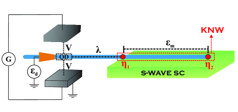
Figure 1: Sketch of the experimental setup, based on the recent experiment performed by M.T.Deng et al. Deng et al. (2016). A piece of semiconductor nanowire is placed on a s-wave superconductor (SC) material. In this semiconductor-superconductor segment, by considering suitable Zeeman field and spin-orbit coupling, a topological KNW emerges, giving rise to overlapped ($\varepsilon_{m}$) MBSs $\eta_{1}$ and $\eta_{2}$ at their edges. A QD (gate-tunable energy $\epsilon_{d}$) between two metallic leads (coupling $V$) is built in the semiconducting segment, where $\eta_{1}$ leaks into (coupling $\lambda$) and can be detected as a ZBP.

We identify the fixed points of the model and perform a renormalization group analysis  Yoshida et al. (2009); Seridonio et al. (2009) to study the crossovers between them and the temperature dependence of the conductance. The leaked Majorana fixed point (LM), accounting for the leakage process  Deng et al. (2016); Vernek et al. (2014), is seen to occur in the vicinity of a characteristic temperature that depends solely on the KNW properties, although the vicinity width depends on the whole set of model parameters. Further, we find rigorously the crossover temperatures and derive an analytic expression describing the universal behavior of the zero-bias conductance along the crossovers. As it happens in the Kondo effect  Yoshida et al. (2009); Seridonio et al. (2009), the universal behavior reveals a more complete signature of the physical system.

Model and fixed points.—Assuming that the Zeeman field is large enough in the system, so that we can neglect the transport of spin down electrons through it, we consider the effective model with spinless fermions Liu and Baranger (2011); Ruiz-Tijerina et al. (2015), whose Hamiltonian is given by

$$H = \sum_{k,\alpha=U,L}\epsilon_{k}c_{k,\alpha}^{\dagger}c_{k,\alpha}+V\sum_{k,\alpha=U,L}\left(c_{k,\alpha}^{\dagger}d+d^{\dagger}c_{k,\alpha}\right)$$ (1)

$$+ \epsilon_{d}d^{\dagger}d+i\epsilon_{m}\eta_{1}\eta_{2}+\sqrt{2}\lambda(d-d^{\dagger})\eta_{1},$$

where the first term describes the conduction electrons in the upper (U) and lower (L) leads. We assume half-filled conduction bands in the particle-hole symmetric regime, with a constant density of states equal to $\rho$, $-D\leq\epsilon_{k,\alpha}\leq D$ and Fermi energy equal to zero. The QD here has only one energy state $\epsilon_{d}$ that is hybridized with the conduction states in the leads through the second term in the Hamiltonian, resulting in a linewidth $\Gamma=\pi\rho V^{2}$. We assume here symmetric coupling to the leads. The KNW is assumed to be in the topological phase with two MBSs at its ends ($\eta_{i}=\eta_{i}^{\dagger}$, $\eta_{i}\eta_{i}=1/2$), with an overlap amplitude $\epsilon_{m}\sim e^{-L/\xi}$ between them, where $L$ is the length of the KNW and $\xi$ is the superconductor coherence length. The last term in the Hamiltonian represents the coupling between the MBS $\eta_{1}$ and the QD single state.

We consider now even and odd conduction states, $e_{k}=(c_{k,U}+c_{k,L})/\sqrt{2}$ and $o_{k}=(c_{k,U}-c_{k,L})/\sqrt{2}$ and also the nonlocal fermionic operators $b=(\eta_{1}+i\eta_{2})/\sqrt{2}$ and $b^{\dagger}=(\eta_{1}-i\eta_{2})/\sqrt{2}$ ($\left\{b,b^{\dagger}\right\}=1,\left\{b,b\right\}=0$), to rewrite the model Hamiltonian as

$$H = \sum_{k}\epsilon_{k}\left(e_{k}^{\dagger}e_{k}+o_{k}^{\dagger}o_{k}\right)+\sqrt{2}V\sum_{k}\left(e_{k}^{\dagger}d+d^{\dagger}e_{k}\right)+\epsilon_{d}d^{\dagger}d$$ (2)

$$+ \epsilon_{m}\left(b^{\dagger}b-\frac{1}{2}\right)-\lambda(d^{\dagger}b+b^{\dagger}d+d^{\dagger}b^{\dagger}+bd),$$

where the odd conduction states are decoupled from the QD and the number of fermions is not conserved.

The zero-bias conductance as a function of the temperature $T$ can be calculated fromYoshida et al. (2009)

$$G(T)=\frac{2e^{2}}{h}\pi\Gamma\left[\frac{1}{k_{B}T}\frac{1}{Z}\sum_{n,m}\frac{|\langle n|d|m\rangle|^{2}}{e^{\beta E_{n}}+e^{\beta E_{m}}}\right]$$ (3)

or, alternatively, we can also rewrite Eq. (3) as Haug and Jauho (2008)

$$G(T)=\frac{2e^{2}}{h}\Gamma\int_{-\infty}^{\infty}\>\text{{Im}}\{G_{d,d}(\omega)\}\left(\frac{\partial f}{\partial\omega}\right)\>d\omega,$$ (4)

where $f(\omega)$ is the Fermi-Dirac function. The QD Green’s function can be promptly obtained from the equation of motion Haug and Jauho (2008) procedure, leading to

$$G_{d,d}(\omega)=\frac{C(\omega)}{A(\omega)C(\omega)-B^{2}(\omega)},$$ (5)

where $A(\omega)=\omega-\epsilon_{d}+2i\Gamma-B,$ $C(\omega)=\omega+\epsilon_{d}+2i\Gamma-B$ and

$$B(\omega) = \frac{2\lambda^{2}\omega}{\omega^{2}-\epsilon_{m}^{2}},$$ (6)

that reproduces the well-known Green’s function for a QD side-coupled to a topological KNW found in Ref.[Liu and Baranger, 2011], here expressed differently for convenience once we target to show the system universality.

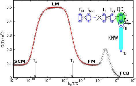
Figure 2: Zero-bias conductance as a function of the temperature in logarithmic scale for $\epsilon_{d}=0.1D$, $\Gamma=0.005\pi D$, $\lambda=0.0008D$, $\epsilon_{m}=5\times 10^{-8}D$. The model parameters were carefully chosen to make the several fixed points very clear. Continuous lines are given by Eqs. (13) and (17) with crossover temperatures $T_{1}$ (Eq. (10)) and $T_{2}$ (Eq. (11)). The inset pictorially shows the Majorana representation of the problem in the leaked Majorana (LM) fixed point, considering a tight-binding description of the conduction band, comprising two uncoupled zig-zag chains of Majorana fermions (blue circles). Majorana fermions $\eta_{1}$ and $\zeta_{2}$ are strongly coupled and removed from the system (see the horizontal arrow). One of the Majorana fermion chains gives rise to half of the single-particle excitations of the free conduction band, while the other chain, coupled to the Majorana fermion $\zeta_{1}$, gives rise to half of the single-particle excitations of the $\epsilon_{d}=0$ resonant level model. This implies a conductance equal to half of that in such resonant level model, explaining the characteristic value 0.5 $e^{2}/h$ in the LM fixed point.

For a vanishing coupling $\lambda$ between the QD and the KNW or for $\epsilon_{m}\to\infty$, so that the fermionic state $b$ becomes empty, we end up with a simple resonant level model. For non-vanishing coupling $\lambda$ and $\epsilon_{m}=0$ (infinite KNW), we can find from Eqs. (4) and (5) that the zero-bias conductance through the QD approaches 0.5 $e^{2}/h$ at $\omega=0$, when the temperature $T\to 0$, whatever the values of $\epsilon_{d}$ and $\Gamma$, being a signature of the leakage of the MBS $\eta_{1}$ into the QDVernek et al. (2014). The problem is that any nonzero $\epsilon_{m}$ makes the conductance change to its resonant level model value

$$G_{0}=\frac{e^{2}}{h}\frac{4\Gamma^{2}}{\epsilon_{d}^{2}+4\Gamma^{2}}=\frac{e^{2}}{h}\leavevmode\nobreak\ \sin^{2}(\delta)$$ (7)

in the limit of zero temperature, where $\delta$ is the phase-shift at the Fermi level. This fact prompt us to a more detailed investigation of the temperature dependence of the conductance.

Results and Discussion.— Fig. 2 is clarifying. At high temperatures, when we can effectively consider both $\lambda$ and $\epsilon_{m}$ equal to zero, the conductance approaches $G_{0}\approx 0.09$ $e^{2}/h$. Then, as the temperature is lowered, the coupling finally emerges, leading to a crossover from a conductance equal to $G_{0}$ towards 0.5 $e^{2}/h$. This value remains stable in a certain temperature range. At some point, however, the tiny energy $\epsilon_{m}$ dominates and the MBSs become strongly coupled, yielding a new crossover ending with $G_{0}$ recovered. This final crossover resembles the Kondo effect Yoshida et al. (2009); Seridonio et al. (2009), where a localized spin is screened by the conduction electrons in spite of how weak can be the coupling between them. If the coupling is very small, the crossover will occur at a extremely low Kondo temperature and eventually can become unobserved. Analogously, in our case, if the KNW is long enough $(\epsilon_{m}\to 0)$, the last crossover can be shifted to very low temperatures, allowing the observation of an essentially stable conductance value equal to 0.5 $e^{2}/h$. As it happens in the Kondo effect, more relevant than particular values of some physical properties in the $T\to 0$ limit is the universal behavior of these physical properties during the crossover as some parameter is changed, typically the temperature. Below, we recognize explicitly the accounted fixed points and then proceed to the analysis concerning the temperature dependence of the conductance.

Free conduction band (FCB) fixed point. This corresponds to do $V=\epsilon_{d}=\lambda=\epsilon_{m}=0$ in the model Hamiltonian. Both QD level and nonlocal fermionic level $b$ are detached from the conduction band and can be empty or occupied, so that any energy is fourfold degenerate. The excitations are those in a free conduction band. The system would be close to this fixed point at temperatures $k_{B}T\gg\Gamma,\epsilon_{d},\lambda,\epsilon_{m}$, where the conductance goes to zero. Since the temperature must necessarily be lower than the effective superconducting gap in the KNW, this fixed point will not be observed in general.

Free Majorana fermions (FM) fixed point. In this case, $\lambda=\epsilon_{m}=0$ and the resulting resonant level model must be considered in the limit $k_{B}T\ll\Gamma$. The energies are twofold degenerate, since the nonlocal fermionic level $b$ can be empty or occupied. The excitations in the conduction band have a phase-shift $\delta$, with $\cot\delta=\epsilon_{d}/2\Gamma$.

Strongly coupled Majorana fermions (SCM) fixed point. Here, we regard $\epsilon_{m}\to\infty$. The MBSs become strongly coupled and the nonlocal fermionic level $b$ remains empty. The system becomes the resonant level model, with the same conductance and same excitations as in the FM fixed point, but without degeneracy.

Leaked Majorana fermion (LM) fixed point: This corresponds to do $\lambda\to\infty$ in the model Hamiltonian. From Eq. (1), the MBSs $\eta_{1}$ and $\zeta_{2}=i(d^{\dagger}-d)/\sqrt{2}$ become infinitely coupled, leading to a nonlocal fermionic level with infinite energy, that remains empty. But, we still have the MBS $\zeta_{1}=(d^{\dagger}+d)/\sqrt{2}$ in the QD, so that the leaked Majorana fixed point is described by the following Hamiltonian:

$$H_{LM} = \sum_{k}\epsilon_{k}e_{k}^{\dagger}e_{k}+V\sum_{k}\left(e_{k}^{\dagger}\zeta_{1}+\zeta_{1}e_{k}\right).$$ (8)

Essentially, the MBS has leaked from the KNW edge into the QD Vernek et al. (2014); Deng et al. (2016). However, it is coupled to the even conduction states so that this leaking process will reach the conduction band.

With the MBS $\zeta_{1}$ at the QD level and $\eta_{2}$ at the other far edge of the KNW, we introduce a new fermionic operator, $a=(\zeta_{1}+i\eta_{2})/\sqrt{2}$, to rewrite $H_{LM}$ as

$$H_{LM}=\sum_{k}\epsilon_{k}e_{k}^{\dagger}e_{k}+\frac{V}{\sqrt{2}}\sum_{k}\left(e_{k}^{\dagger}a+e_{k}^{\dagger}a^{\dagger}+\mathrm{h.c.}\right).$$ (9)

As discussed in the caption of Fig. 2 and explained in detail in the supplemental material, one half of the single-particle excitations of $H_{LM}$ are of free-conduction band type and another half of them are of $\epsilon_{d}=0$ resonant level model type. Only the last set of excitations can contribute to the conductance, leading to the characteristic value of 0.5 $e^{2}/h$ as $T\to 0$.

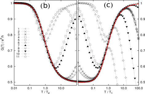
Figure 3: (a) Zero-bias conductance as a function of the temperature in logarithmic scale for 11 different model parameter pairs $(\lambda,\epsilon_{m})$. In all curves, $\epsilon_{d}=0$ and $\Gamma=\pi 0.005\leavevmode\nobreak\ D$. The inset shows the distribution of the corresponding crossover temperatures $T_{1}$ and $T_{2}$ (Eqs. (10) and (11)). Curves 1-5 have the same $\lambda$ and the same $T_{1}$. As $T_{2}$ increases (with $\epsilon_{m}^{2}$), approaching $T_{1}$, the crossovers will merge at some point, and the LM fixed point ceases to be achieved. Curves 6-11 have the same $\epsilon_{m}$ and their minima between the crossovers are approximately at the same point (Eq. (12)). As $\lambda$ increases, $T_{1}$ rises and $T_{2}$ lowers, broadening the LM fixed point plateau. (b) and (c) Conductance as a function of $T/T_{2}$ and $T/T_{1}$, respectively. The points collapse into the continuous lines in Eq. (13) with ${\mathcal{H}}(t)$ in Eq. (17). In (b), when $T_{1}$ is not much higher than $T_{2}$, deviations from the universal curve will start at low temperatures. In (c), deviations at $T<T_{1}$ occur when $T_{2}$ is not much lower than $T_{1}$ while deviations at $T>T_{1}$ occur when $T_{1}$ is not much smaller than $\Gamma/k_{B}$.

Now we turn to the problem of carefully identifying universal behavior in the zero-bias conductance. In Fig. 3a, we show the conductance for different sets of model parameters. We have used $\epsilon_{d}=0$ and $\Gamma=\pi 0.005\leavevmode\nobreak\ D$, changing $\epsilon_{m}$ and $\lambda$. Therefore, we have conductance $G_{0}=1.0\leavevmode\nobreak\ e^{2}/h$ in the FM and SCM fixed points. It is clear from Fig. 3a that the crossovers occur around parameter-dependent temperatures $T_{1}$ (between the FM fixed point and the LM fixed point) and $T_{2}$ (between the LM fixed point and the SCM fixed point). We have found from the numerical results that

$$k_{B}T_{1}=\frac{2}{\Gamma}\frac{\lambda^{2}}{\left[1+\left(\frac{\epsilon_{d}}{2\Gamma}\right)^{2}\right]},$$ (10)

and

$$k_{B}T_{2}=\frac{\Gamma}{2}\left[1+\left(\frac{\epsilon_{d}}{2\Gamma}\right)^{2}\right]\left(\frac{\epsilon_{m}}{\lambda}\right)^{2}.$$ (11)

Physically, it is clear that $T_{1}$ must increase with $\lambda$ and that $T_{2}$ must increase with $\epsilon_{m}$. Differently from a naive expectation, we have $T_{2}\propto\epsilon_{m}^{2}$, not $\epsilon_{m}$. Except for the resonant case, $\epsilon_{d}=0$, $T_{1}$ and $T_{2}$ are not monotonic functions of $\Gamma$. With the remaining parameters fixed, when $\Gamma=|\epsilon_{d}|/2$, $T_{1}$ is maximum and $T_{2}$ is minimum. For $\epsilon_{d}=0$, increasing the hybridization between the QD and the conduction band lowers $T_{1}$, since the QD level mixes with the continuum of states, making the coupling with the Majorana fermion $\eta_{1}$ less effective, and increases $T_{2}$, once the Majorana fermion that leaked to the conduction band around the LM fixed point will couple to the Majorana fermion $\eta_{2}$ more easily with a strong hybridization.

Scaling the temperature by $T_{2}$ or $T_{1}$, the crossover portions of the different curves in Fig. 3a collapse into the same curve as shown in Figs. 3b and 3c. In addition, we have

$$\sqrt{T_{1}T_{2}}=\epsilon_{m}/k_{B},$$ (12)

that means the plateau at 0.5$e^{2}/h$ in the conductance will be centered at $T\sim\epsilon_{m}/k_{B}$, being well defined only if $T_{2}\ll\epsilon_{m}/k_{B}\ll T_{1}$. From Figs. 3b and 3c, we see that the temperature must be changed by at least two orders of magnitude to complete the crossover, what demands $T_{1}>100T_{2}$ to clearly have the system in the LM fixed point. The ratio $T_{1}/T_{2}=(k_{B}T_{1}/\epsilon_{m})^{2}$ depends on all parameters, what helps to tune it large enough.

In general, we expect Yoshida et al. (2009); Seridonio et al. (2009) that the conductance between a low-temperature fixed-point ($G=G_{l}$) and a high-temperature fixed-point ($G=G_{h}$) be given by

$$G=\frac{G_{l}+G_{h}}{2}+\frac{G_{l}-G_{h}}{2}{\mathcal{H}}\left(\frac{T}{T^{\star}}\right),$$ (13)

where ${\mathcal{H}}(t)$ is a universal function characteristic of the crossover and $T^{\star}$ is the crossover temperature. In the present case, we have found that the same universal function describes the crossover between SCM and LM fixed points and that between LM and FM fixed points.

In order to determine ${\mathcal{H}}(t)$ analytically, we consider the SCM$\to$LM crossover, for instance, and assume $T_{2}\ll\epsilon_{m}\ll T_{1}$ to have the crossovers well separated. For temperatures $T\sim T_{2}\ll\epsilon_{m}/k_{B}$, an inspection in Eq. (4) shows that only energies $\omega\ll\epsilon_{m}$ are important, so we have $B(\omega)\approx-2\left(\frac{\lambda}{\epsilon_{m}}\right)^{2}\omega$ in Eq. (6). Introducing $r=\frac{\lambda^{2}}{\epsilon_{m}^{2}}$, $x=\frac{\epsilon_{d}}{2\Gamma}$ and $z=\frac{\omega}{k_{B}T_{2}}$, we have from Eq. (5) that

$$G_{d,d}\approx-\frac{1}{4\Gamma(1+x^{2})}\left[\frac{z(1+x^{2})+2x+i2}{1-iz}\right],$$ (14)

where we have exploited that $r\gg 1$ and that $2rk_{B}T_{2}=\Gamma(1+x^{2})$. Substituting Eq. (14) into Eq. (4), defining $t=T/T_{2}$ and changing to the variable $u=\omega/k_{B}T=z/t$, we get

$$\frac{G(T)}{e^{2}/h}=\int_{-\infty}^{\infty}\left[\frac{\frac{u^{2}t^{2}}{2}+\frac{G_{0}}{e^{2}/h}}{1+u^{2}t^{2}}\right]\frac{e^{u}}{\left(e^{u}+1\right)^{2}}\leavevmode\nobreak\ du.$$ (15)

If we add and subtract $\frac{1}{2}\left(\frac{G_{0}}{e^{2}/h}+\frac{1}{2}\right)$ to the term between brackets in (15) and use that $\int_{-\infty}^{\infty}\frac{e^{u}}{\left(e^{u}+1\right)^{2}}du=1$, we will finally obtain

$$\frac{G(T)}{e^{2}/h}=\frac{1}{2}\left(\frac{G_{0}}{e^{2}/h}+\frac{1}{2}\right)+\frac{1}{2}\left(\frac{G_{0}}{e^{2}/h}-\frac{1}{2}\right){\mathcal{H}}(t),$$ (16)

with the universal function given by

$${\mathcal{H}}(t)=\int_{-\infty}^{\infty}\left[\frac{1-u^{2}t^{2}}{1+u^{2}t^{2}}\right]\frac{e^{u}}{\left(e^{u}+1\right)^{2}}\leavevmode\nobreak\ du.$$ (17)

Conclusions.—In summary, we have determined the universal behavior of the zero-bias conductance for the simple spinless model in Eq. (1) along the crossovers connected to the LM fixed point. This enlarges the signature of the MBS in the end of the KNW and can help to reveal its presence when the LM fixed point is not fully achieved. Even with a finite KNW, it may be possible to set up the model parameters to have $T_{1}\gg T_{2}$ and a reasonably large temperature range with conductance close to 0.5$e^{2}/h$. We expect that the current findings offer additional guides to identify signatures of MBSs in solid state setups.

Acknowledgments.—We thank the funding Brazilian agencies CNPq (307573/2015-0), CAPES and São Paulo Research Foundation (FAPESP) - grant: 2015/23539-8.

References

- Kitaev (2003) A. Y. Kitaev, Annals of Physics 303, 2 (2003).
- Sarma et al. (2015) S. D. Sarma, M. Freedman, and C. Nayak, npj Quantum Information 1, 15001 (2015).
- Nayak et al. (2008) C. Nayak, S. H. Simon, A. Stern, M. Freedman, and S. D. Sarma, Rev. Mod. Phys. 80, 1083 (2008).
- Alicea et al. (2011) J. Alicea, Y. Oreg, G. Refael, F. Von Oppen, and M. P. Fisher, Nat. Phys. 7, 412 (2011).
- Leijnse and Flensberg (2012) M. Leijnse and K. Flensberg, Semicond. Sci. Technol. 27, 124003 (2012).
- Alicea (2012) J. Alicea, Rep. Prog. Phys. 75, 076501 (2012).
- Beenakker (2013) C. Beenakker, Annu. Rev. Condens. Matter Phys. 4, 113 (2013).
- Fu and Kane (2008) L. Fu and C. L. Kane, Phys. Rev. Lett. 100, 096407 (2008).
- Sau et al. (2010) J. D. Sau, R. M. Lutchyn, S. Tewari, and S. Das Sarma, Phys. Rev. Lett. 104, 040502 (2010).
- Alicea (2010) J. Alicea, Phys. Rev. B 81, 125318 (2010).
- Lutchyn et al. (2010) R. M. Lutchyn, J. D. Sau, and S. Das Sarma, Phys. Rev. Lett. 105, 077001 (2010).
- Oreg et al. (2010) Y. Oreg, G. Refael, and F. von Oppen, Phys. Rev. Lett. 105, 177002 (2010).
- Linder et al. (2010) J. Linder, Y. Tanaka, T. Yokoyama, A. Sudbø, and N. Nagaosa, Phys. Rev. Lett. 104, 067001 (2010).
- Cook and Franz (2011) A. Cook and M. Franz, Phys. Rev. B 84, 201105 (2011).
- Nadj-Perge et al. (2013) S. Nadj-Perge, I. K. Drozdov, B. A. Bernevig, and A. Yazdani, Phys. Rev. B 88, 020407 (2013).
- Kitaev (2001) A. Y. Kitaev, Physics-Uspekhi 44, 131 (2001).
- Mourik et al. (2012) V. Mourik, K. Zuo, S. M. Frolov, S. Plissard, E. Bakkers, and L. Kouwenhoven, Science 336, 1003 (2012).
- Das et al. (2012) A. Das, Y. Ronen, Y. Most, Y. Oreg, M. Heiblum, and H. Shtrikman, Nat. Phys. 8, 887 (2012).
- Deng et al. (2012) M. Deng, C. Yu, G. Huang, M. Larsson, P. Caroff, and H. Xu, Nano Lett. 12, 6414 (2012).
- Churchill et al. (2013) H. Churchill, V. Fatemi, K. Grove-Rasmussen, M. Deng, P. Caroff, H. Xu, and C. M. Marcus, Phys. Rev. B 87, 241401 (2013).
- Finck et al. (2013) A. Finck, D. Van Harlingen, P. Mohseni, K. Jung, and X. Li, Phys. Rev. Lett. 110, 126406 (2013).
- Deng et al. (2014) M. Deng, C. Yu, G. Huang, M. Larsson, P. Caroff, and H. Xu, Sci. Rep. 4, 7261 (2014).
- Nadj-Perge et al. (2014) S. Nadj-Perge, I. K. Drozdov, J. Li, H. Chen, S. Jeon, J. Seo, A. H. MacDonald, B. A. Bernevig, and A. Yazdani, Science 346, 602 (2014).
- Higginbotham et al. (2015) A. P. Higginbotham, S. M. Albrecht, G. Kiršanskas, W. Chang, F. Kuemmeth, P. Krogstrup, T. S. Jespersen, J. Nygård, K. Flensberg, and C. M. Marcus, Nat. Phys. 11, 1017 (2015).
- Zhang et al. (2016) H. Zhang, Ö. Gül, S. Conesa-Boj, K. Zuo, V. Mourik, F. K. de Vries, J. van Veen, D. J. van Woerkom, M. P. Nowak, M. Wimmer, et al., arXiv preprint arXiv:1603.04069 (2016).
- Deng et al. (2016) M. T. Deng, S. Vaitiekenas, E. B. Hansen, J. Danon, M. Leijnse, K. Flensberg, J. Nygård, P. Krogstrup, and C. M. Marcus, Science 354, 1557 (2016).
- Liu and Baranger (2011) D. E. Liu and H. U. Baranger, Phys. Rev. B 84, 201308 (2011).
- Cao et al. (2012) Y. Cao, P. Wang, G. Xiong, M. Gong, and X.-Q. Li, Phys. Rev. B 86, 115311 (2012).
- Lee et al. (2013) M. Lee, J. S. Lim, and R. López, Phys. Rev. B 87, 241402 (2013).
- Vernek et al. (2014) E. Vernek, P. H. Penteado, A. C. Seridonio, and J. C. Egues, Phys. Rev. B 89, 165314 (2014).
- López et al. (2014) R. López, M. Lee, L. Serra, and J. S. Lim, Phys. Rev. B 89, 205418 (2014).
- Leijnse (2014) M. Leijnse, New J. Phys. 16, 015029 (2014).
- Liu et al. (2015) D. E. Liu, M. Cheng, and R. M. Lutchyn, Phys. Rev. B 91, 081405 (2015).
- Li et al. (2015) Z.-Z. Li, C.-H. Lam, and J. You, Sci. Rep. 5 (2015).
- Ruiz-Tijerina et al. (2015) D. A. Ruiz-Tijerina, E. Vernek, L. G. D. da Silva, and J. Egues, Phys. Rev. B 91, 115435 (2015).
- Yoshida et al. (2009) M. Yoshida, A. C. Seridonio, and L. N. Oliveira, Phys. Rev. B 80, 235317 (2009).
- Seridonio et al. (2009) A. C. Seridonio, M. Yoshida, and L. N. Oliveira, Phys. Rev. B 80, 235318 (2009).
- Haug and Jauho (2008) H. Haug and A.-P. Jauho, Quantum Kinetics in Transport and Optics of Semiconductors, Vol. 123 (Springer-Verlag Berlin Heidelberg, 2008).