Leaked Lyman $\alpha$ emission: an indicator of the size of quasar absorption outflows

Abstract

The galactocentric distance of quasar absorption outflows are conventionally determined using absorption troughs from excited states, a method hindered by severely saturated or self-blended absorption troughs. We propose a novel method to estimate the size of a broad absorption line (BAL) region which partly obscures an emission line region by assuming virialized gas in the emission region surrounding a supermassive black hole with known mass. When a spiky Lyman $\alpha$ $\lambda 1216$ line emission is present at the flat bottom of the deep N v $\lambda 1240$ absorption trough, the size of BAL region can be estimated. We have found 3 BAL quasars in the SDSS database showing such Lyman $\alpha$ lines. The scale of their BAL outflows are found to be 3-26 pc, moderately larger than the theoretical scale (0.01-0.1pc) of trough forming regions for winds originating from accretion discs, but significantly smaller than most outflow sizes derived using the absorption troughs of the excited states of ions. For these three outflows, the lower limits of ratio of kinetic luminosity to Eddington luminosity are 0.02%-0.07%. These lower limits are substantially smaller than that is required to have significant feedback effect on their host galaxies.

1. Introduction

Quasar outflow, as an essential component of the quasar structure, has been routinely invoked as a primary feedback mechanism to explain the growth of super-massive black holes (SMBHs), evolution of the host galaxies, enrichment of the intergalactic medium (IGM), cluster cooling flows, and the luminosity function of quasars, e.g. (Silk & Rees, 1998; Loeb et al., 2004; Springel et al., 2005; Haiman et al., 2006; Novak et al., 2011; Soker & Meiron, 2011; Choi et al., 2014; Nims et al., 2015; Ciotti et al., 2016). These outflows often manifest themselves as blueshifted broad absorption lines (BALs) in 20-40% of quasars (Hewett & Foltz, 2003; Dai et al., 2008). To assess whether BAL outflows are an effective agent of quasar feedback, it is necessary to determine their average mass flow rate and associated kinetic luminosity. Theoretical studies and simulations suggested that kinetic power of order of only  1% of the Eddington luminosity is deemed sufficient for significant feedback effects on the host galaxy, e.g. (Scannapieco & Oh, 2004; Hopkins et al., 2006; Hopkins & Elvis, 2010), which now becomes the benchmark number for observational comparisons.

The spatial extents of BAL outflows are challenging to measure, which have been found to span several orders of magnitude (ranging from parsec to kilo-parsec scales), though pc vs. kpc controversial results are sometimes reported in the literature, e.g. see the comments by (Lucy et al., 2014). The controversy in the outflow radius directly leads to large uncertainty in the outflow enegetics, rendering it pointless to determine whether effective feedback is at work. The most direct method to pin down the outflow radius is using spatially resolved spectroscopy, especially integral field unit (IFU) spectroscopy, e.g. (Barbosa et al., 2009; Riffel & Storchi-Bergmann, 2011; Rupke & Veilleux, 2013; Liu et al., 2013a, b, 2014, 2015; Wylezalek et al., 2017; Bae et al., 2017), but for high-redshift ($z>2$) BAL quasars, the realistic approach is deriving the galactocentric distance of the outflow (R) from ionization parameter ($U=Q/[4\pi R^{2}n_{\rm H}c]$), where the hydrogen number density $n_{\rm H}$ can be determined from the absorption lines of the excited states of ions (e.g. Fe II*, Si II*, S IV*). During the last decade or so, the outflow radii have been measured for a number of individual quasars using density-sensitive absorption lines from excited levels, e.g. (Hamann et al., 2001; Arav et al., 2008, 2015; Chamberlain et al., 2015). It should be noted that when the utilized absorption lines are broad and blended, and/or when severe saturation (commonly) takes place, this approach, relying on photoionization modeling and geometric assumptions, introduces nontrivial uncertainty.

Complementary to the conventional approaches, here we propose a method to estimate the spatial location of the outflow for a special class of BAL quasars. As illustrated in Fig. 1, a number of quasars show a narrow (or even spiky) Lyman $\alpha$ emission line at the bottom of broad and close-to-black N v absorption trough, indicating that the Lyman $\alpha$  line emission is leaked from the emission line region, which is otherwise virtually compleletly obscured by the BAL region/outflow (the concept of a BAL region and that of a BAL outflow are used interchangeably throughout the paper, because the detailed physical difference between them is subtle; even if the difference is nontrivial, their spatial scales are expected to be of the same order of magnitude). With this physical picture constructed, the size of a BAL region can be derived by assuming virialized line-emitting gas surrounding a super-massive black hole with known mass (detailed in Section 4).

In this paper, we present three $z=3$ quasars charaterizing close-to-black N v  absorption troughs and spiky leaked Lyman $\alpha$ emission lines, and demonstrate how our method is applied on them. As a result of a comprehensive search in the SDSS-III DR12 database (see Section 2 for details), these objects are among the most representative examples of this special class of BAL quasars. This paper is structured as follows. In §2, we describe the selection of the quasars from the SDSS-III database, and the basic properties of their spectroscopy data. The analysis of their spectra is presented in §3, and the size and energetics of their BAL outflows are measured in §4 and §5. We further discuss the origin of these spiky Lya emission lines in §6, before a summary given in §7. Throughout this work, we adopt a standard $\Lambda$CDM cosmology with $\Omega_{\Lambda}=0.7$ ,$\Omega_{M}=0.3$ and $H_{0}=70$ km s^-1  Mpc^-1.

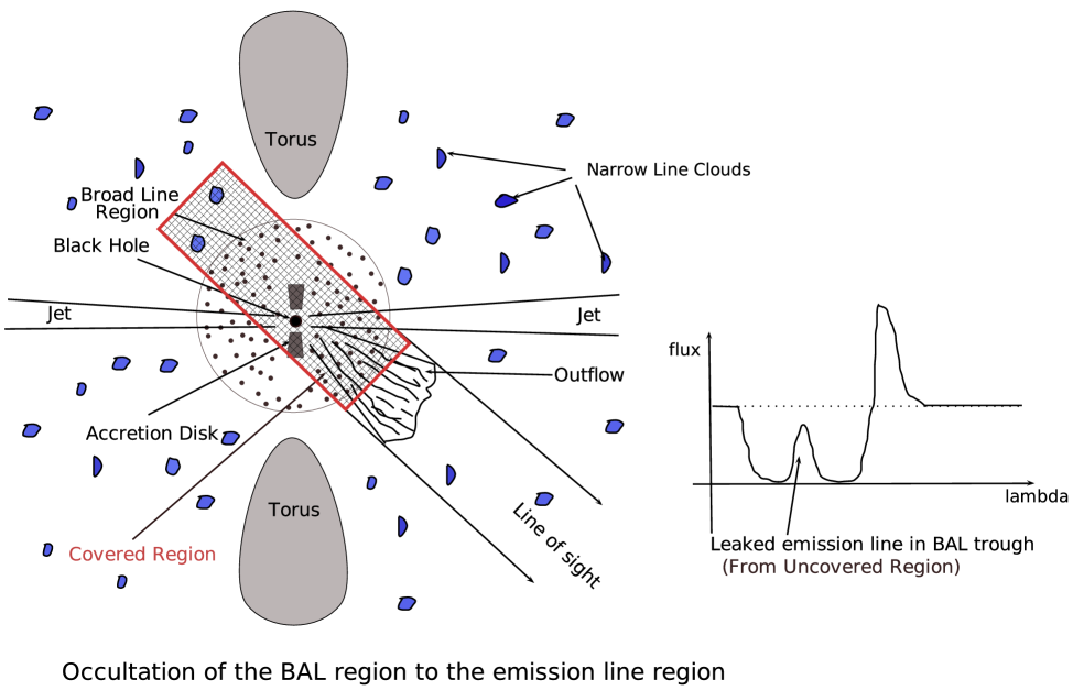
Figure 1.— Cartoon of the occultation of the BALR to the emission line region: The uncovered part of emission source will show leaked emission lines in the BAL troughs. The size of outflow can be estimated by measuring the width of leaked emission line by assuming virialized gas in the emission region surrounding a supermassive black hole with known mass.

2. Sample description

The Baryon Oscillation Spectroscopic Survey (BOSS), part of the third generation of the Sloan Digital Sky Survey (SDSS-III), uses the dedicated 2.5-m wide-field telescope at Apache Point Observatory near Sacramento Peak in Southern New Mexico to conduct an imaging and spectroscopic survey. This catalog is a product of the intensive visual inspection of SDSS optical spectra from the twelfth data release (DR12; (Alam et al., 2015)) undertaken by (Pâris et al., 2016) . About 10% (29580) of these quasars show BALs, whose trough-by-trough properties have been measured and catalogued in the DR12Q_BAL table by the same group. For our purposes, the visually inspected redshift ($Z_{\rm vi}$), the median signal-to-noise ratio over the rest-frame wavelength range 1650-1750Å, and the maximum and minimum velocity that encloses the C iv absorption trough (VMAX_C iv and VMIN_C iv, respectively) are the key parameters for our sample selection.

The Lyman $\alpha$ $\lambda 1216$ emission line is situated on the blue wing of N v $\lambda 1240$ emission line with a blueshift velocity of 5806 ${\rm km\,s}^{-1}$, and our sample quasars are expected to show the Lyman $\alpha$-N v region in their SDSS spectra, translating to a requirement of $Z_{\rm vi}>2.0$. Among the entire DR12Q_BAL parent sample, we find 1945 quasars with sufficiently high redshifts. Meanwhile, C iv and N v are expected to have comparable column densities, because their ionization potentials (64.5 eV vs. 97.9 eV) and abundances (carbon is only 4.8 times higher) are not significantly dissimilar. Adopting a criterion of VMAX_C iv $>6500~{}{\rm km\,s}^{-1}$ and VMIN_C iv $<5000~{}{\rm km\,s}^{-1}$ further reduces the sample size to 290.

Through visual inspection and spectrum fitting, we find 58 quasars whose C IV troughs show flat bottoms with approximately zero flux. In this paper, we analyze the 3 objects demonstrating the most prominent spiky feature in their Lya emission line on top of the N v absorption trough, and are thus consistent with our physical interpretion that these lines are leaked out from the BAL absorption region. The basic information of these sample quasars are reported in Table 1, with visually inspected redshifts $Z_{\rm vi}$=2.9-3.1, as reported by (Pâris et al., 2016).

3. SPECTRAL ANALYSIS

3.1. Redshift calibration

We observe a systematic blueshift in the Lyman $\alpha$, N v, Si iv and C iv, when the visually determined redshift $Z_{\rm vi}$, highlighting the necessity of a line redshift calibration, so that the kinematics of the line-emitting ionized gas can be reliably characterized. Although most of the emission lines (especially the high-ionization broad emission lines) are found to be systematically shifted in the quasar spectra (Grandi et al., 1982; Wilkes et al., 1986; Tytler & Fan, 1992; Laor et al., 1995; McIntosh et al., 1999; Vanden Berk et al., 2001), an apparent anti-correlation between the velocity shifts and the ionization potential is seen in both broad and narrow lines (Vanden Berk et al., 2001). From the above anti-correlation, we deduce that the low-ionization Fe II $\lambda 1785.4$ line has an average shift of at the most 385  km s^-1 , negligible in the composite quasar spectra created by (Vanden Berk et al., 2001). Here note that, using Fe II $\lambda 1785.4$ line as redshift reference is new. It can be useful for high-z BAL QSOs, where no other lines in the optical spectrum can be used as a reference.

Employing a single Gaussian profile, we fit the Fe II $\lambda 1785.4$ line (Fig. 2). The resultant calibrated redshifts are 2.909, 3.067, 3.046 for the three quasars (Table. 1). Applying these redshifts, the centroids of the Lyman $\alpha$, N v, and C iv lines all show minimal shifts ($<200~{}{\rm km\,s}^{-1}$).

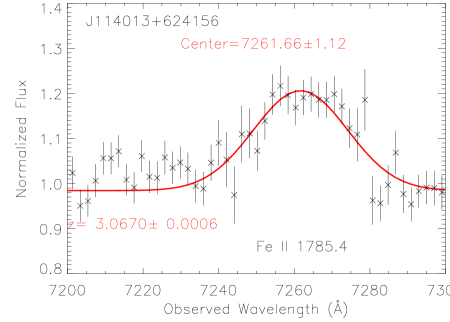
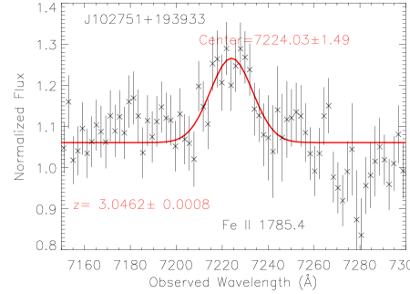
Figure 2.— Using a single Gauss function to fit the low-ionization Fe II $\lambda 1785.4$ line to give a calibration for the quasar redshift.

3.2. Fitting the spectra

The sample quasar spectra all have been corrected for Galactic extinction, adopting the extinction curve of (Cardelli et al., 1989) (IR band; UV band) and (O’Donnell et al., 1994)(optical band) with $R_{\rm V}$ = 3.1. The $A_{\rm V}$ values of these SDSS BAL quasars are derived from the SpecPhotoAll table in SDSS. To reliably characterize the continuum and delineate it from the C iv, N v BAL troughs, we fit the spectra using 165 unabsorbed quasar templates given by (Wang et al., 2015), which were drived from 38,377 non-BAL quasars with $1.5<z<4.0$ and $SNR_{\rm 1350}>10$ in SDSS Data Release 7 (DR7). Following (Wang et al., 2015), we scale their templates using a scale factor, which is a double power-law function of the rest-frame wavelength,

$$S_{\lambda}=A[1]\left(\frac{\lambda}{2000\AA}\right)^{A[2]}+A[3]\left(\frac{\lambda}{2000\AA}\right)^{A[4]}$$ (1)

where coefficients (A[1],A[3]) and exponents(A[2],A[4]) are pinned down by minimizing the $\chi^{2}$ value. This fitting spans a wavelength range of 1050 to 2850Å  and we add a additional Gaussian component at the Lyman $\alpha$, N v, Si iv and C iv locations to the unabsorbed templates to improve the fits therein. Also, we iteratively mask spectral pixels lower than the model with a significance of $\geq 3\sigma$ on the blue side of Lyman $\alpha$, N v, Si iv, C iv to exclude possible absorption contamination from the Lyman $\alpha$ forest. The fitting procedure is demonstrated in Fig. 3.

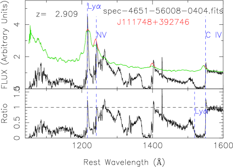
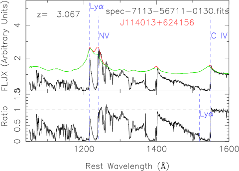
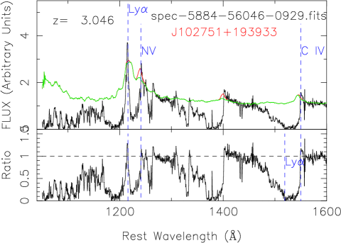
Figure 3.— Top panel: unabsorbed template fit to the spectra of the three SDSS quasars. The cyan line shows the scaled best matched template, while the red line has additional Gaussians to account for emission lines. Bottom panel: The ratio of observation to fitting spectrum. The blue dot line mark Lyman $\alpha$ $\lambda 1216$ position in the N v BAL trough and the corresponding position in the C iv trough.

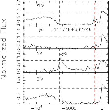
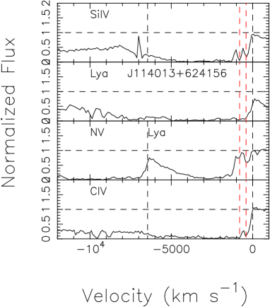
Figure 4.— Put C iv, N v, Lyman $\alpha$ and Si iv ions BAL troughs together in the velocity space. The black vertical dotted lines mark the position of red component of other ions or Lyman $\alpha$. The red ones mark the position of the two narrow absorbtions. The velocity of the first narrow troughs relative to the peak of Lyman $\alpha$ (or red component of other ion) is about 600 ${\rm km\,s}^{-1}$ and 400 ${\rm km\,s}^{-1}$ for J111748+392746 and J114013+624156 respectively. The velocity gap of the two narrow troughs is about 500 ${\rm km\,s}^{-1}$ for all the ions in both two quasars.

Fitting and normalizing the quasar spectra facilitate our characterization of the N v-Lyman $\alpha$ region. As shown in Fig. 3, the bottom of the N v trough (in correspondence to C iv) is appoximately flat and the spectral flux is nearly zero (lower than 5% of the continuum level). In our physical interpretion of the data (see Fig. 1), the Lyman $\alpha$ spike is leaked line emission from the unobscured emission region. When C iv,N v(Lyman $\alpha$ included) and Si iv BAL troughs are plotted in the velocity space (Fig. 4), we find two barely separated narrow absorption features at -1000 km s^-1  to -400 km s^-1   in at least two of the four ions in both J1117+3927 and J1140+6241.

3.3. Characterizing the Lyman $\alpha$ emission line

3.3.1 C iv absorption trough

The residual flux of the N v BAL trough likely caused by partical covering, (e.g. Arav et al., 1999) or small residuals can be scattered light as well because BAL troughs are more polarized, (e.g. Ogle et al., 1999). Although approximating zero, it needs to be fully removed to recover the line profile of the Lyman $\alpha$ emission. For this purpose, we use the spectrum of the C iv BAL resudial flux as a template to fit the that of the NV BAL trough. We note that the velocity separation of the N v1238.8, 1242.8Å doublet (966 km s^-1 ) is larger than that of the C iv 1548.2, 1550.8Å doublet (503 km s^-1 ), and the latter is strongly blended.

The complex velocity structure of C iv prevents us from structuring a simplestic model (e.g. a single Gaussian), but we have the freedom to introduce a sophisiticated mathematical formalism, since a phenominalogical (rather than physical) modeling is sufficient for our purposes. Here, this formalism is set to be the superposition of a Gaussian on a 5th-order polynomial. We increase the fitting weight by a factor of 2 for the bottom of the CIV trough, so that the detailed structure in this region receives more attention from the fits. As a result, the C iv velocity profiles are well represented and de-blended by the best-fit models resulting from this procedure (Fig. 5).

For the resonance doublet C iv 1548.2, 1550.8Å  the ratio of their oscillator strengths ($f_{\rm blue}$ = 0.19 and $f_{\rm red}$ = 0.095, respectively) , renders an optical depth ratio of $f_{\rm blue}/f_{\rm red}$ close to 2 (see Equation 9). Partial covering obscuration is generally assumed to interprete non-black absorption troughs, for which $I(v)=1-C(v)+C(v)e^{-\tau(v)}$, where $C(v)$ is the covering factor and $\tau(v)$ is the optical depth of the ion at velocity v (Arav et al., 1999; Hall et al., 2003). However, for our sample quasars with flat and nearly black troughs, we find it sufficient to derive the apparent optical depth, which is introduced only as a proxy for our procedure of analysis. Hence, for simplicity and with effectiveness, we take $C(v)$=1 throughout the absorption trough, and the above formalism retrogrades to the classical Beer-Lambert law,

$$I(v)=e^{-\tau(v)}.$$ (2)

3.3.2 N v absorption trough

As shown in Fig. 6, the blue wing of the Lyman $\alpha$ emission line (inside the N v BAL trough) is an interplay between N v absorption and the intrinsic Lyman $\alpha$ emission (bluer than -6458 km s^-1 , the velocity separation of the N v red line and Lya in our de-redshifted spectrum). To remove the residual flux in the N v  trough, we scale the apparent optical depths of the C iv trough by a factor of $k$, fit the data to $I_{\rm fit}(v)=e^{-k\tau_{\rm{\rm C}\,{\sc iv}\ }(v)}$, and perform the standard $\chi^{2}$ minimization procedure. The best-fit k values we obtain are $0.65\pm 0.01,0.88\pm 0.02$ and$~{}0.58\pm 0.02$ for SDSS J1117+3927, J1140+6241 and J1027+1939, respectively. In Fig. 6, the blue line depicts the ’intrinsic profile’ of the Lyman $\alpha$ emission as a result of subtracting the best-fit N v resudial flux profile from the observed spectrum.

3.3.3 Lyman $\alpha$ emission line

We use two methods to measure the width of the leaked Lyman $\alpha$ emission line.

(1) Using a single Gaussian to fit the Lyman $\alpha$ line (Fig. 7): we mask the blue wing of Lyman $\alpha$ where presents the narrow absorbtion components (SDSS J1117+3927 and J1140+6241) when doing the Gaussian fitting.

(2) Directly measuring FWHM of Lyman $\alpha$ without fitting (non-parametric).

The results of the two methods are listed in Table 1. Due to the narrow absorptions, the FWHMs of directly measurement are significantly smaller than that of Gaussian fitting for J1117+3927 and J1140+6241.

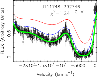
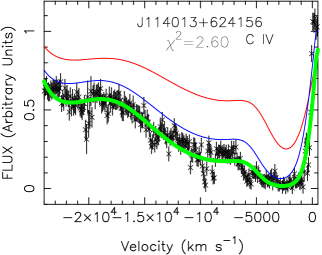
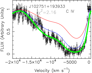
Figure 5.— Using a Gaussian plus a five order polynomial function for the optical depth to fit the C iv1548.2, 1550.8Å doublet blended BAL trough. Red and blue line repesent the red, blue component of the doublet while the cyan one is for the total trough. We use a covering factor c=1 throughout the trough. The minimizing $\chi^{2}$ of the fitting are 1.24, 2.60, 2.16 for J1117+3927, J1140+6241 and J1027+1939, respectively.

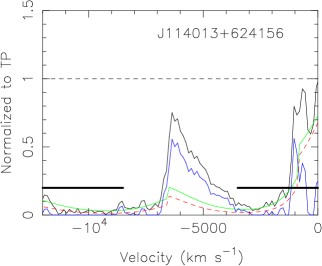
Figure 6.— The fitting of the resudial flux of N v trough (cyan solid line) using the extracted template of C iv  BAL trough (red dotted line). The black solid line is the original normalized resudial flux and the blue one is the intrinsic (subtracted) normalized resudial flux. The fitting window is selected to be away from the leaked Lyman $\alpha$ (black horizontal line).

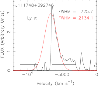
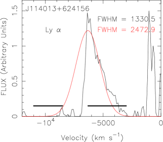
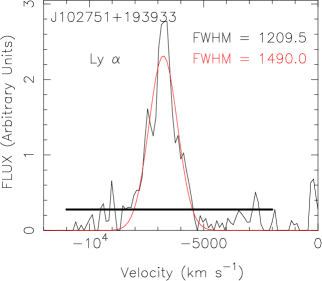
Figure 7.— Two methods to measure the width of the leaked Lyman $\alpha$ emission line: (1) Using a single Gaussian to fit the leaked Lyman $\alpha$ line (red). (2) Directly measuring FWHM of Lyman $\alpha$ without fitting (black). We mask the blue wing of Lyman $\alpha$ where presents the narrow absorbtion components (SDSS J111748+392746 and J114013+624156) when doing the Gaussian fitting. The black horizontal line shows fitting windows.

4. Results

4.1. Methodology

The radii of the BAL regions (BALRs) can be estimated from the width of the the leaked Lyman $\alpha$ emission. Assumption that the line-emitting gas in this region is fully varialized, the radius of the Lyman $\alpha$ emission line region (i.e. the BALR) is related to the line width through

$$R_{\rm BALR}=\frac{GM_{\rm BH}}{fv^{2}}$$ (3)

where the velocity dispersion of the virialized gas $v={\rm FWHM}/(2\sqrt{2\ln{2}})$, G is $6.67\times 10^{-8}cm^{3}g^{-2}s^{-2}$ (gravitational constant). $f$ is a virial factor that depends on the geometry and dynamics e.g., (Kashi et al., 2013; Waters et al., 2016), with the average values $\langle f\rangle\approx 1-6$ by observations (McLure & Dunlop, 2004; Onken et al., 2004; Woo et al., 2010; Grier et al., 2013). Here we adopt $f=4.31$ measured from a sample containing 30 AGNs e.g. see (Grier et al., 2013). Fiducial values for a typical black hole mass and a typical Lyman $\alpha$ line width are $10^{9}M_{\odot}$ and $3000~{}{\rm km\,s}^{-1}$, respectively, rendering a distance to the central black hole of $\sim$ 0.61 pc. The BALR sizes of the three sample quasars can then be estimated as follows:

$$R_{\rm BALR}=\frac{M_{\rm BH}}{10^{9}M_{\odot}}\times(\frac{3000~{}{\rm km\,s}^{-1}}{{\rm FWHM}})^{2}\times 0.61~{}pc.$$ (4)

4.2. $M_{\rm BH}$ and outflow sizes

For our quasars, the SDSS spectrum covers the rest-frame wavelength range of 1100-2500Å, and the conventional approach of estimating the bolometric luminosity using the 5100Å  luminosity is inapplicable. However, the optical-UV spectrum of a quasar can be represented by a power law, $L_{v}\sim v^{\alpha}$, where the power index alpha is roughly between 0 and -1 (e.g. Natali et al. 1998). Adopting $\alpha=-1$ results in a constant lambda $L_{\lambda}$ value across the UV-optical region, and our measured $\lambda L_{\lambda}$ at 2000Å directly translates to $\lambda L_{\lambda}$ (5000Å)=[3.4, 5.4, 2.4]$\times 10^{46}ergs~{}s^{-1}$, respectively. Applying a bolometric correction factor of 9 (Kaspi et al., 2000) on $\lambda L_{\lambda}$ (5000Å), we find their bolometric luminosity to be [3.1, 4.9, 2.2]$\times 10^{47}ergs~{}s^{-1}$, respectively (Table 1).

The well-established radius-luminisoity relation allows for deriving the radius of a broad emission line region $R_{\rm BLR}$ using the following formulism:

$$R_{\rm BLR}=\alpha\left(\frac{\lambda_{\rm 5100}L_{\rm 5100}}{10^{44}ergs~{}s^{-1}}\right)^{\beta}$$ (5)

where the parameters, $\alpha$ and $\beta$ are $30.2\pm 1.4$ and $0.64\pm 0.02$ given in (Greene & Ho, 2005). So, the $R_{\rm BLR}$ are $1.06\pm 0.08$ pc, $1.43\pm 0.09$ pc and $0.85\pm 0.09$ pc for the three quasars respectively. It should be pointed out that, UV luminosity is better than optical one for R-L relation if there is no extinction because it is the ionizing continuum causes emission lines. Since high-luminosity quasars have $L_{\rm Bol}/L_{\rm Edd}\sim$ 1, their MBH values are about [2.4, 3.9, 1.7]$\times 10^{9}M_{\odot}$, correspondingly. Note that, there are black hole formulaes for UV continuum/line, especially for Mg ii $\lambda 2798$ (Wang et al., 2009) which is not in the wavelength range of our quasar spectrums. Inserting these numbers into Equation (3), we find the following outflow radii (Table 1):

(1) J1117+3927: 2.96 pc (Gaussian fit) or 25.62 pc (non-parametric);

(2) J1140+6241: 3.50 pc (Gaussian fit) or 12.09 pc (non-parametric);

(3) J1027+1939: 4.26 pc (Gaussian fit) or 6.46 pc (non-parametric).

As mentioned in §3.3.3, due to the narrow absorptions, the FWHMs of directly measurement are significantly smaller than that of Gaussian fitting for J1117+3927 and J1140+6241. As a result, the $R_{\rm BLR}$ deduced from FWHM of directly measurement is larger than that from Gaussian fitting. We take the $R_{\rm BLR}$ deduced from FWHM of directly measurement as an upper limit. These results indicate that sizes of the BAL regions of the three sample quasars are roughly two orders of magnitude larger than the theoretically predicted sizes of the trough forming region (0.01-0.1 pc) for accretion disc line-driven winds (Murray et al., 1995; Proga, Stone & Kallman, 2000), but is comparable to those determined from BAL variability (Capellupo et al., 2011; Shi et al., 2016). Two outflow components are also found to be between 1 and 10 pc from the central source (de Kool et al., 2002a, b). They lie closer to the central source than most of the other outflow which deduced using troughs from excited states e.g. (Hamann et al., 2001; Arav et al., 2008, 2015; Chamberlain et al., 2015).

Table 1Main physical characteristic parameters of the three BAL quasars. Z is the redshift measured using Fe II $\lambda 1785.4$ line. The values in the brackets of ${\rm FWHM}$ (Lyman $\alpha$) and $R_{\rm BALR}$ are for the directly measuring FWHM of Lyman $\alpha$ without fitting (non-parametric).

NAME	$Z$	$L_{\rm Bol}$	$M_{\rm BH}$	FWHM (Lyman $\alpha$)	$R_{\rm BALR}$	$R_{\rm BLR}$
		$(10^{47}ergs~{}s^{-1})$	$(10^{9}M_{\odot})$	(km s-1 )	(pc)	(pc)
J111748+392746	2.909	$3.08\pm 0.22$	2.44	2134.1(725.7)	2.96(25.62)	1.06$\pm 0.08$
J114013+624156	3.067	$4.88\pm 0.20$	3.87	2472.9(1330.5)	3.50(12.09)	1.43$\pm 0.09$
J102751+193933	3.046	$2.16\pm 0.22$	1.71	1490.0(1209.5)	4.26(6.46)	0.85$\pm 0.09$

Table 2Main physical parameters of the BAL outflow in the three BAL quasars.

NAME	$V_{\rm centroid}$ (C iv)	$N_{\rm{\rm C}\,{\sc iv}\ }~{}$	$N_{\rm{\rm Si}{\textsc{iv}}}~{}$	$N_{\rm{\rm Al}{\textsc{iii}}}~{}$	$N_{\rm H}~{}$	$\dot{M}$	$\dot{E_{\rm k}}/L_{\rm Edd}$
	$({\rm km\,s}^{-1})$	$(\hbox{cm${}^{-2}$})$	$(\hbox{cm${}^{-2}$})$	$(\hbox{cm${}^{-2}$})$	$(\hbox{cm${}^{-2}$})$	$(M_{\odot}\,{\rm yr}^{-1})$	(%)
J111748+392746	11543	$\geq 7.62E+16$	$\geq 1.28E+16$	$1.09E+15$	$\geq 3.55E+21$	$\geq 3.45$	$\geq 0.05$
J114013+624156	11526	$\geq 3.87E+16$	$\geq 1.08E+16$	$6.65E+14$	$\geq 1.58E+21$	$\geq 1.75$	$\geq 0.02$
J102751+193933	7698	$\geq 2.10E+16$	$\geq 1.10E+16$	$1.76E+15$	$\geq 9.12E+21$	$\geq 8.68$	$\geq 0.07$

5. Outflow energetics

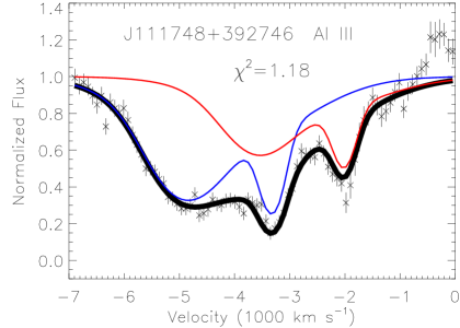
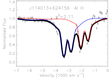
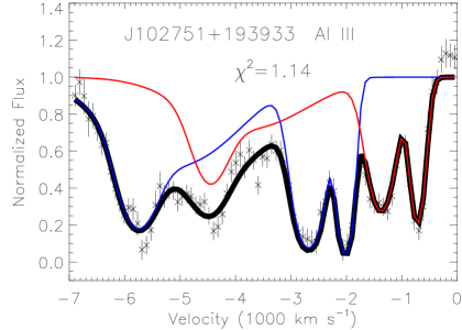
Figure 8.— Using two to four Gaussian functions as the form of optical depth of the Al iii1854.7, 1862.8Å doublet blended BAL trough. Considering the flat and deep absorbtion of C iv and Si iv trough, we take the covering factor c=1 throughout the trough when doing the fit. The red line repesents the red component while blue repesents the blue one. The minimizing $\chi^{2}$ of the fitting are 1.18, 2.11, 1.14 for J1117+3927, J1140+6241 and J1027+1939, respectively.

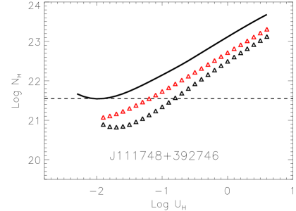
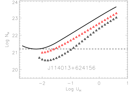
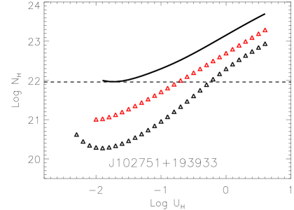
Figure 9.— $N_{\rm H}-U_{\rm H}$ plane plot showing the photoionization solution using the UV-soft SED for gas with one solar metallicity. The black triangle repesents the lower limit of $N_{\rm H}$ from $N_{\rm{\rm C}\,{\sc iv}\ }$ while red triangle from $N_{\rm{\rm Si}{\textsc{iv}}}$. The black line represents the $N_{\rm H}$ deduced from $N_{\rm{\rm Al}{\textsc{iii}}}$. The dotted line repesents the finally lower limit of $N_{\rm H}$ which used to calculate the lower limit of the mass-flow rate $\dot{M}$ and kinetic luminosity $\dot{E_{\rm k}}$ of the outflow.

Quantifying the effectiveness of AGN feedback requires an estimate of the mass flow rate $\dot{M}$ and kinetic luminosity $\dot{E}_{k}$ of the outflow. Adopting the conventional assumption of a partial thin shell geometry ($\Delta R/R\ll 1$), these quantities are given by (Borguet et al., 2012),

$$\dot{M}=4\pi\Omega R\mu m_{p}N_{\rm H}v$$ (6)

$$\dot{E_{k}}=2\pi\Omega R\mu m_{p}N_{\rm H}v^{3}$$ (7)

, where R is the distance from the outflow to the central source, $\Omega$ is the global covering fraction of the outflow, $\mu$= 1.4 is the mean atomic mass per proton, $m_{p}$ is the mass of the proton, $N_{\rm H}$ is the total hydrogen column density of the absorber, and $v$ is the radial velocity of the outflow. Here, we adopt the weighted centroid velocity of C iv BAL trough, i.e., the mean of the velocities where each data point is weighted with its distance from the normalized continuum level (Filiz Ak et al., 2013). From the Equation (3) and (7), getting the

$$\begin{split}\dot{E_{\rm k}}/L_{\rm Edd}&=\frac{\Omega}{0.2}\times(\frac{v}{10^{4}~{}{\rm km\,s}^{-1}})^{3}\times\frac{N_{\rm H}}{10^{21}\hbox{cm${}^{-2}$}}\\ &\times(\frac{3000~{}{\rm km\,s}^{-1}}{{\rm FWHM}})^{2}\times 0.004323\%.\end{split}$$ (8)

Although we derived the black hole mass in the last section, it should be noted that $M_{\rm BH}$ does not appear in Equation (8), so the accuracy of estimating $M_{\rm BH}$ does not affect the characterization of the outflow energetics. The fiducial number $\Omega$ $\sim$ 0.2 is derived from the convention that the fraction of BAL quasars among all quasars (defined from the C iv absorption trough) statistically represents the average fraction of $4\pi$ covered by the solid angle of the outflow (see Introduction). The total hydrogen column density $N_{\rm H}$ could be deduced from the observed column density of C iv, Si iv and Al iii  through photoionization modeling(e.g. CLOUDY; (Ferland et al., 1998)).

We use a combination of 2-4 Gaussians to fit the optical depth profile of the BAL trough as a result of the blended Al iii1854.7, 1862.8Å. As we did for the C iv trough, we adopt a covering factor of C=1 thoughout the entire Al iii  trough when it is fitted to the Gaussians. Integrating the optical depth over the trough yields the ionic column density (Savage & Sembach, 1991):

$$N_{ion}=\frac{3.7679\times 10^{14}\hbox{cm${}^{-2}$}}{\lambda f}\int{\tau(v)dv}$$ (9)

where $\lambda$ and $f$ are the wavelength and oscillator strength of the transition, and the velocity is the unit of km s^-1 . It should be noted that the above phenomelogical calculation likely gives a lower limit of the C iv and Si iv column densities, regarding the broad and close-to-black absorption that is likely saturated. The results are summarized in Table 2.

In order to further derive the hydrogen column density of the absorbers (again, actually a lower limit) from that of C iv, Si iv and Al iii, we perform a series of photoionization simulations using version c13.03 of CLOUDY (Ferland et al., 2013). We adopt a typical density $n_{e}$ = $10^{6}\hbox{cm${}^{-3}$}$, considering that gas ionization is not sensitive to electron density at a given ionization parameter U e.g. (Wang et al., 2015). We compute a set of models over the range of ionization parameter $-3\leq LogU\leq 1$ using a step of $\Delta LogU$ = 0.1. Due to the fact that the three sample quasars in this paper are all high-luminosity, radio-quiet quasars, we use the UV-soft SED for this quasar type following (Dunn et al., 2010) to characterize the continuum of ionizing photons. We assume the solar metalicity for these quasars, though previous discussion in the literature has shown insiginificant effects when the metalicity is varied in a reasonable range (Chamberlain et al., 2015).

The results are plotted on the $N_{\rm H}$-$U_{\rm H}$ plane in Fig. 9. The black triangles depict the lower limit of $N_{\rm H}$ derived from $N_{\rm{\rm C}\,{\sc iv}\ }$, while red triangles are those from $N_{\rm{\rm Si}{\textsc{iv}}}$. We adopt the lower limit of $N_{\rm H}$ derived from Al iii (the dotted line), which is used to calculate and constrain $\dot{M}$ and $\dot{E_{\rm k}}$ of the outflow. Correspondingly, the lower limit of $\dot{M}$ is 1.4, 1.0 and 6.1 $M_{\odot}\,{\rm yr}^{-1}$ for J1117+3927, J1140+6241 and J1027+1939, and the lower limit of $\dot{E_{\rm k}}/L_{\rm Edd}$ is 0.05%, 0.02%, 0.07%, respectively. It is worth mentioning that (Kurosawa, Proga & Nagamine, 2009) predicted the quasar outflow efficiencies are as low as found in our work.

6. Discussion: the origin of spiky Lyman $\alpha$ emission lines

In this paper, we interpret the spiky Lyman $\alpha$ emission lines on top of flat, nearly black N v BAL troughs to be leaked emission from the broad line region. The line width of the Lyman $\alpha$ lines is $\sim$ 2000 km s^-1  (comparable to that of broad emission lines), which, in our physical picture, orginates from the roughly virialized line-emitting gas. In this section, we discuss on other possible origins of these Lyman $\alpha$ spikes, and assess their pausibility.

(1) Galactic disks: the Lyman $\alpha$ line width of our sample quasars are all over $10^{3}$ km s^-1 , which safely rules out the possibility that the spiky Lyman $\alpha$ originates from galactic disks, for which the ionized gas produced by star formation activity generally has a velocity dispersion of the order $<\sim 100-200~{}{\rm km\,s}^{-1}$ e.g. (Liu et al., 2013b).

(2) Ambient gas/outflow: an outflow that extends on galactic (or even intergalactic) scales may produce a pair of superbubbles, as is seen in a number of quasars e.g. (Greene et al., 2012; Liu et al., 2013b). The wall of the superbubbles is generally thin, and its relatively low velocity dispersion may cause a spiky component in the Lyman $\alpha$ emission line. In fact, both recombination and resonant scattering may produce Lyman $\alpha$  photons, but the large column density of the BAL troughs in the three sample quasars indicates their outflows to be highly optically thick to the hydrogen-ionizing continuum. In that case, the chance that the ionizing continuum photons escape to (inter-)galactic scales in the directions of BAL outflows (i.e. our line of sight) and produces the recombined or scattered Lyman $\alpha$ emission is expected to be minimal. Admittedly, the possibility cannot be completely ruled out that the spectrum also collects Lyman $\alpha$ light from galaxy-wide superbubbles outside the (strictly defined) line of sight, but the rather low surface brightness feature generally found in superbubbles does not appear to be consistent with the strong Lyman $\alpha$ emission seen in our sample. In addition, the line can be resonantly scattered line by a rotating outflow (Wang et al., 2007), in this case, the line width is of order the rotation velocity, which can be either sub or super-Keplerian depends where there are strong magnetic fields.

(3) Intergalactic gas in cold accretion: numerical simulations predict that the rapid replenishment of gas for star formation may have proceeded in the ”cold accretion” mode (Keres et al., 2005; Dekel et al., 2009). The cold gas accreted into galaxies in the cosmic web can be photoionized by the quasar, or even the neutral hydrogen therein may scatter the quasar radiation to give rise to Lyman $\alpha$ emission. The origin of circumgalactic gas remains unconclusive, but evidence has been found indicating the combination of pristine gas accreted in this manner and gas reprocessed by AGN and/or star formation activity e.g. (Lehner et al., 2013; Chen, 2016). Although a challenging task, the extended Lyman $\alpha$ emission from cosmic-web nebulae has been detected in $z\sim~{}2$ to 3 quasars (Cantalupo et al., 2014; Martin et al., 2014; Hennawi et al., 2015). However, the velocity dispersion of the intergalactic gas in cold accretion is expected to be $<50~{}{\rm km\,s}^{-1}$, smaller than our targets by about 2 orders of magnitude. In addition, our searching in the SDSS archive leads to no spotted quasars within a distance of $\sim$ 2.4 Mpc from our targets, while clustered quasars hint for the existence of a giant nebula and a proto-cluster (Hennawi et al., 2015).

7. SUMMARY

In this paper, we present an estimate of the size of BAL outflows for a special type of quasars, whose N v absorption troughs are wide, flat and nearly black, enclosing a spiky Lyman $\alpha$ emissin line. Our interpretation is that the spiky Lyman $\alpha$  emission is leaked from the BAL material obscuring the broad emission line region.

Our systematic search in the SDSS DR12Q catalog renders 3 quasars prominently characterizing the above feature. Under the assumption that the line-emitting gas is virialized, we estimate that the FWHM of the Lyman $\alpha$ spikes ($\sim$ 2000 km s^-1 ) indicates a size of their outflows to be of the order 3-26 parsecs, similar or moderately larger than the theoretically investigated trough forming region (0.01-0.1 pc) for accretion disc line-driven winds (Murray et al., 1995; Proga, Stone & Kallman, 2000). The lower limits of $\dot{E_{\rm k}}/L_{\rm Edd}$ are 0.02%-0.07% which are substantially smaller than that is required to have significant feedback effect on their host galaxies.

3/58 of quasars with flat C iv absorption troughs show spiky Lyman $\alpha$ emission line, it may indicate that the small scale BALRs are rare. Although the outflow radii of a number of individual quasars measured using density-sensitive absorption lines from excited levels often find tens to 100-1000 pc scales, this contraversy has been long-standing in this field (Lucy et al., 2014), and no available data that facilitate a direct comparison for our quasar sample.

8. ACKNOWLEDGMENTS

Authors thank the anonymous referee for constructive comments and suggestions for improving the clarity of the manuscript. We acknowledge the financial support by the Strategic Priority Research Program ”The Emergence of Cosmological Structures” of the Chinese Academy of Sciences (XDB09000000), NSFC (NSFC-11233002, NSFC-11421303, U1431229) and National Basic Research Program of China (grant No. 2015CB857005).

Guilin Liu is supported by the National Thousand Young Talents Program of China, and acknowledges the grant from the National Natural Science Foundation of China (No. 11673020 and No. 11421303) and the Ministry of Science and Technology of China (National Key Program for Science and Technology Research and Development, No. 2016YFA0400700).

References

- Alam et al. (2015) Alam S. et al., 2015, ApJS, 219, 12A
- Arav et al. (1999) Arav N., de Kool M., Becker R. H., Laurent-Muehleisen S. A., White R. L., Price T., Gregg M. D., 1999, AAS, 195, 1805
- Arav et al. (2008) Arav N., Moe M., Costantini E., Korista K. T., Benn C., Ellison S., 2008, ApJ, 681, 954
- Arav et al. (2015) Arav N. et al., 2015, A&A, 577, 37
- Bae et al. (2017) Bae, H. J., Woo, J. H., Karouzos, M., et al., 2017, ApJ, 837, 91
- Barbosa et al. (2009) Barbosa, F. K. B., Storchi-Bergmann, T., Cid Fernandes, R., Winge, C., & Schmitt, H. 2009, MNRAS, 396, 2
- Borguet et al. (2012) Borguet B. C. J., Edmonds D., Arav N., Dunn J., Kriss G. A., 2012, ApJ, 751, 107
- Cantalupo et al. (2014) Cantalupo S., Arrigoni-Battaia F., Prochaska J. X., Hennawi J. F., Madau P., 2014, Natur, 506, 63
- Capellupo et al. (2011) Capellupo D. M., Hamann F., Shields J. C., Rodríguez Hidalgo P., & Barlow, T. A. 2011, MNRAS, 413, 908
- Cardelli et al. (1989) Cardelli J. A., Clayton G. C., & Mathis J. S., 1989, ApJ, 345, 245
- Chamberlain et al. (2015) Chamberlain C., Arav N., Benn C., 2015, MNRAS, 450, 1085C
- Chen (2016) Chen, Hsiao-Wen, 2016, arXiv:1612.00872
- Choi et al. (2014) Choi E. Naab T., Ostriker J. P., Johansson P. H., Moster B. P., 2014, MNRAS, 442, 440
- Ciotti et al. (2016) Ciotti L., Pellegrini S., Negri A., Ostriker J. P., 2016, arXiv:1608.03403
- Dai et al. (2008) Dai X., Shankar F., Sivakoff G. R., 2008, ApJ, 672, 108
- de Kool et al. (2001) de Kool M, Arav N, Becker R H., Gregg M D., White R L., Laurent-Muehleisen S A., Price T, Korista K T., 2001, ApJ, 548, 609
- Dekel et al. (2009) Dekel A., Birnboim Y., Engel G., Freundlich J., Goerdt T., Mumcuoglu M., Neistein E., Pichon C., Teyssier R., Zinger E., 2009, Natur, 457, 451
- de Kool et al. (2002a) de Kool M., Becker R. H., GreggM. D., White R. L., Arav N., 2002a, ApJ, 567, 58
- de Kool et al. (2002b) de Kool M., Becker R. H., Arav N., GreggM. D., White R. L., 2002b, ApJ, 570, 514
- Dunn et al. (2010) Dunn J. P. et al., 2010, ApJ, 709, 611
- Grandi et al. (1982) Grandi, S. A., 1982, ApJ, 255, 25
- Greene & Ho (2005) Greene, J. E., Ho, L. C., 2005, ApJ, 630, 122
- Greene et al. (2012) Greene, J. E., Zakamska, N. L., Smith, P. S., 2012, ApJ, 746, 86
- Grier et al. (2013) Grier, C. J., Martini, P., Watson, L. C., et al. 2013, ApJ, 773, 90
- Ferland et al. (1998) Ferland, G. J., Korista, K. T., Verner, D. A., Ferguson, J. W., Kingdon, J. B., Verner, E. M., 1998, PASP, 110, 761F
- Ferland et al. (2013) Ferland, G. J., Porter, R. L., van Hoof, P. A. M., Williams, R. J. R., Abel, N. P. , Lykins, M. L., Shaw, G., Henney, W. J., and Stancil, P. C.. The 2013 Release of Cloudy. Revista Mexicana de Astronomia y Astrofisica, 49:137163
- Filiz Ak et al. (2013) Filiz Ak, N., Brandt, W. N., Hall, P. B., et al. 2013, ApJ, 777, 168
- Haiman et al. (2006) Haiman, Z., 2006, MmSAI, 7, 629H
- Hamann et al. (2001) Hamann, F. W., Barlow, T. A., Chaffee, F. C., Foltz, C. B., Weymann, R. J., 2001, ApJ, 550, 142
- Hall et al. (2003) Hall, P. B., Hutsem’ekers, D., Anderson, S. F., et al. 2003, ApJ, 593, 189
- Hennawi et al. (2015) Hennawi, J. F.,Prochaska J. X., Cantalupo S, Arrigoni-Battaia F., 2015, Sci, 348, 779
- Hewett & Foltz (2003) Hewett, P. C., Foltz, C. B., 2003, AJ, 125, 1784
- Hopkins et al. (2006) Hopkins, P. F., Hernquist, L., Cox T. J., Di Matteo, T., Robertson, B., Springel, V., 2006, ApJS, 163, 1
- Hopkins & Elvis (2010) Hopkins P. F., Elvis M., 2010, MNRAS, 401, 7
- Kashi et al. (2013) Kashi, A., Proga, D., Nagamine, K., Greene, J., Barth, A. J., 2013, ApJ, 778, 50
- Kaspi et al. (2000) Kaspi, Shai, Smith, Paul S., Netzer, Hagai, Maoz, Dan, Jannuzi, Buell T., Giveon, Uriel, 2000, ApJ, 533, 631
- Keres et al. (2005) Keres, D., Katz, N., Weinberg D. H., Dave R., 2005, MNRAS, 363, 2
- Kurosawa, Proga & Nagamine (2009) Kurosawa, R., Proga, D. & Nagamine, K. 2009, ApJ, 707, 823
- Laor et al. (1995) Laor, A., Bahcall, J. N., Jannuzi, B. T., Schneider, D. P. & Green, R. F. 1995, ApJS, 99, 1
- Lehner et al. (2013) Lehner, N., Howk, J. C., Tripp, T. M., Tumlinson, J., Prochaska, J. X., O’Meara J. M., Thom, C., Werk, J. K., Fox, A. J., Ribaudo, J., 2013, ApJ, 770, 138
- Liu et al. (2013a) Liu, G., Zakamska N. L., Greene J. E., Nesvadba N. P. H., & Liu, X. 2013a, MNRAS, 430, 2327
- Liu et al. (2013b) Liu, G., Zakamska N. L., Greene J. E., Nesvadba N. P. H., & Liu, X. 2013b, MNRAS, 436, 2576
- Liu et al. (2014) Liu, G., Zakamska, N. L., & Greene, J. E. 2014, MNRAS, 442, 1303
- Liu et al. (2015) Liu, G., Arav, N., & Rupke, D. S. N. 2015, ApJS, 221, 9
- Loeb et al. (2004) Loeb A., 2004, MNRAS, 350, 725L
- Lucy et al. (2014) Lucy, A. B., Leighly, K. M., Terndrup, D. M., Dietrich, M., Gallagher, S. C., 2014, ApJ, 783, 58
- McIntosh et al. (1999) McIntosh, D. H., Rix, H.-W., Rieke, M. J. & Foltz, C. B. 1999, ApJ, 517, L73
- McLure & Dunlop (2004) McLure, R. J., & Dunlop, J. S. 2004, MNRAS, 352, 1390
- Martin et al. (2014) Martin, D. C., Chang, D., Matuszewski, M., Morrissey, P., Rahman, S., Moore, A., Steidel, C. C., 2014, ApJ, 786, 106
- Murray et al. (1995) Murray N., Chiang J., Grossman S. A., & Voit G. M., 1995, ApJ, 451, 498
- Nims et al. (2015) Nims J., Quataert E., Faucher-Giguere C., 2015, MNRAS, 447, 3612
- Novak et al. (2011) Novak G. S., Ostriker J. P., Ciotti L., 2011, ApJ, 737, 26
- O’Donnell et al. (1994) O’Donnell J. E. et al., 1994, ApJ, 422, 158
- Ogle et al. (1999) Ogle P. M., Cohen M. H., Miller J. S., Tran H. D., Goodrich R. W., Martel A. R., 1999, ApJS, 125, 1
- Onken et al. (2004) Onken, C. A., Ferrarese, L., Merritt, D., et al. 2004, ApJ, 615, 645
- Pâris et al. (2016) Pâris I. et al., 2016, arXiv:1608.06483
- Proga, Stone & Kallman (2000) Proga D., Stone J. M., Kallman T. R., 2000, ApJ, 543, 686
- Riffel & Storchi-Bergmann (2011) Riffel, R. A., & Storchi-Bergmann, T. 2011, MNRAS, 417, 2752
- Rupke & Veilleux (2013) Rupke D. S. N., Veilleux S., 2013, ApJ, 768, 75
- Savage & Sembach (1991) Savage B. D., & Sembach K. R., 1991, ApJ, 379, 245
- Scannapieco & Oh (2004) Scannapieco, E., & Oh, S. P. 2004, ApJ, 608, 62
- Shi et al. (2016) Shi Xiheng, Zhou Hongyan, Shu Xinwen, Zhang Shaohua, Ji Tuo, Pan Xiang, Sun Luming, Zhao Wen, Hao Lei, 2016, ApJ, 819, 99
- Silk & Rees (1998) Silk J., Rees M. J., 1998, A&A, 331, L1
- Soker & Meiron (2011) Soker N., Meiron Y., 2011, MNRAS, 411, 1803
- Springel et al. (2005) Springel V., Di M. T., Hernquist L., 2005, MNRAS, 361, 776
- Tytler & Fan (1992) Tytler, D. & Fan, X. 1992, ApJS, 79, 1
- Vanden Berk et al. (2001) Vanden Berk, Daniel E., et al., 2001, AJ, 12, 549
- Wang et al. (2007) Wang H. Y., Wang T. G., Wang J. X., 2007, ApJS, 168, 195
- Wang et al. (2009) Wang J. G.; Dong X. B, Wang T. G., Ho L. C., Yuan W. M., Wang H. Y, Zhang K., Zhang S. H., Zhou, H. Y., 2009, ApJ, 707, 1334
- Wang et al. (2015) Wang T. G., Yang C. W., Wang H. Y., 2015, ApJ, 814, 150
- Waters et al. (2016) Waters, T., Kashi, A., Proga, D., Eracleous, M., Barth, A. J., Greene, J., 2016, ApJ, 827, 53
- Wilkes et al. (1986) Wilkes B. J. 1986, MNRAS, 218, 331
- Woo et al. (2010) Woo, J. H., Treu, T., Barth, A. J., et al. 2010, ApJ, 716, 269
- Wylezalek et al. (2017) Wylezalek, D., Schnorr Műller, A., Zakamska, N. L., 2017, MNRAS, tmp, 248