Lucid Data Dreaming for Video Object Segmentation

Abstract

Convolutional networks reach top quality in pixel-level video object segmentation but require a large amount of training data ($1k\negmedspace\sim\negmedspace 100k$) to deliver such results. We propose a new training strategy which achieves state-of-the-art results across three evaluation datasets while using $20\times\negmedspace\sim\negmedspace 1000\times$ less annotated data than competing methods. Our approach is suitable for both single and multiple object segmentation.

Instead of using large training sets hoping to generalize across domains, we generate in-domain training data using the provided annotation on the first frame of each video to synthesize (“lucid dream”) plausible future video frames. In-domain per-video training data allows us to train high quality appearance- and motion-based models, as well as tune the post-processing stage. This approach allows to reach competitive results even when training from only a single annotated frame, without ImageNet pre-training. Our results indicate that using a larger training set is not automatically better, and that for the video object segmentation task a smaller training set that is closer to the target domain is more effective. This changes the mindset regarding how many training samples and general “objectness” knowledge are required for the video object segmentation task.

1 Introduction

Figure 1: Starting from scarce annotations we synthesize in-domain data to train a specialized pixel-level video object segmenter for each dataset or even each video sequence.

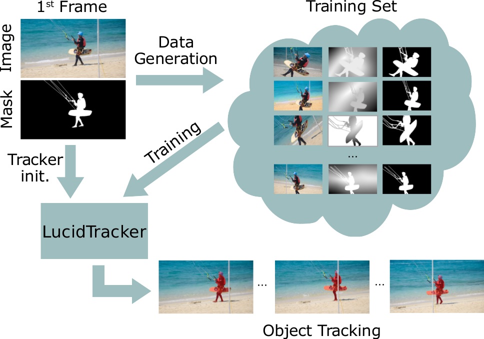
In the last years the field of localizing objects in videos has transitioned from bounding box tracking Kristan2015Iccvw ; Hadfield14d ; Hadfield16d to pixel-level segmentation Li2013Iccv ; Prest2012Cvpr ; Perazzi2016Cvpr ; Vojir2017TechreportVOT16Seg . Given a first frame labelled with the foreground object masks, one aims to find the corresponding object pixels in future frames. Segmenting objects at the pixel level enables a finer understanding of videos and is helpful for tasks such as video editing, rotoscoping, and summarisation.

Top performing results are currently obtained using convolutional networks (convnets) Jampani2016Arxiv ; Caelles2017Cvpr ; Khoreva2017CvprMaskTrack ; Bertinetto2016Arxiv ; Held2016Eccv ; Nam2016Cvpr . Like most deep learning techniques, convnets for video object segmentation benefit from large amounts of training data. Current state-of-the-art methods rely, for instance, on pixel accurate foreground/background annotations of $\sim\negmedspace 2k$ video frames Jampani2016Arxiv ; Caelles2017Cvpr , $\sim\negmedspace 10k$ images Khoreva2017CvprMaskTrack , or even more than $100k$ annotated samples for training Voigtlaender2017OnlineAO . Labelling images and videos at the pixel level is a laborious task (compared e.g. to drawing bounding boxes for detection), and creating a large training set requires significant annotation effort.

In this work we aim to reduce the necessity for such large volumes of training data. It is traditionally assumed that convnets require large training sets to perform best. We show that for video object segmentation having a larger training set is not automatically better and that improved results can be obtained by using $20\times\negmedspace\sim\negmedspace 1000\times$ less training data than previous approaches Caelles2017Cvpr ; Khoreva2017CvprMaskTrack ; Voigtlaender2017OnlineAO . The main insight of our work is that for video object segmentation using few training frames ($1\negmedspace\sim\negmedspace 100$) in the target domain is more useful than using large training volumes across domains ($1k\negmedspace\sim\negmedspace 100k$).

To ensure a sufficient amount of training data close to the target domain, we develop a new technique for synthesizing training data particularly tailored for the pixel-level video object segmentation scenario. We call this data generation strategy “lucid dreaming”, where the first frame and its annotation mask are used to generate plausible future frames of the videos. The goal is to produce a large training set of reasonably realistic images which capture the expected appearance variations in future video frames, and thus is, by design, close to the target domain.

Our approach is suitable for both single and multiple object segmentation in videos. Enabled by the proposed data generation strategy and the efficient use of optical flow, we are able to achieve high quality results while using only $\sim\negmedspace 100$ individual annotated training frames. Moreover, in the extreme case with only a single annotated frame and zero pre-training (i.e. without ImageNet pre-training), we still obtain competitive video object segmentation results.

In summary, our contributions are the following:
1. We propose “lucid data dreaming”, an automated approach to synthesize training data for the convnet-based pixel-level video object segmentation that leads to top results for both single and multiple object segmentation.
2. We conduct an extensive analysis to explore the factors contributing to our good results.
3. We show that training a convnet for video object segmentation can be done with only few annotated frames. We hope these results will affect the trend towards even larger training sets, and popularize the design of video segmentation convnets with lighter training needs.

With the results for multiple object segmentation we took the second place in the 2017 DAVIS Challenge on Video Object Segmentation Pont-Tuset_arXiv_2017 . A summary of the proposed approach was provided online DAVIS2017-2nd . This paper significantly extends DAVIS2017-2nd with in-depth discussions on the method, more details of the formulation, its implementation, and its variants for single and multiple object segmentation in videos. It also offers a detailed ablation study and an error analysis as well as explores the impact of varying number of annotated training samples on the video segmentation quality.

2 Related work

Box tracking

Classic work on video object tracking focused on bounding box tracking. Many of the insights from these works have been re-used for video object segmentation. Traditional box tracking smoothly updates across time a linear model over hand-crafted features Henriques2012Eccv ; breitenstein2009robust ; Hadfield14d . Since then, convnets have been used as improved features Danelljan2015Iccvw ; Ma-ICCV-2015 ; wang2015visual , and eventually to drive the tracking itself Held2016Eccv ; Bertinetto2016Arxiv ; tao2016siamese ; nam2016modeling ; Nam2016Cvpr . Contrary to traditional box trackers (e.g. Henriques2012Eccv ), convnet-based approaches need additional data for pre-training and learning the task.

Video object segmentation

In this paper we focus on generating a foreground versus background pixel-wise object labelling for each video frame starting from a first manually annotated frame. Multiple strategies have been proposed to solve this task.

Box-to-segment: First a box-level track is built, and a space-time grabcut-like approach is used to generate per frame segments Xiao2016Cvpr .

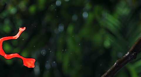
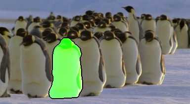
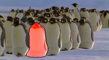
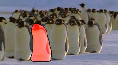
Video saliency: this group of methods extracts the main foreground object pixel-level space-time tube. Both hand-crafted models Faktor2014Bmvc ; Papazoglou2013Iccv or trained convnets TokmakovAS17 ; Jain2017ArxivFusionSeg ; Song_2018_ECCV have been considered. Because these methods ignore the first frame annotation, they fail in videos where multiple salient objects move (e.g. flock of penguins).

Space-time proposals: these methods partition the space-time volume, and then the tube overlapping most with the first frame mask annotation is selected as tracking output Grundmann2010Cvpr ; Perazzi2015Iccv ; Chang2013tsp .

Mask propagation: Appearance similarity and motion smoothness across time is used to propagate the first frame annotation across the video Maerki2016Cvpr ; Wang2017ArxivSTV ; Tsai2016Cvpr . These methods usually leverage optical flow and long term trajectories.

Convnets: following the trend in box tracking, recently convnets have been proposed for video object segmentation. Caelles2017Cvpr trains a generic object saliency network, and fine-tunes it per-video (using the first frame annotation) to make the output sensitive to the specific object of interest. Khoreva2017CvprMaskTrack uses a similar strategy, but also feeds the mask from the previous frame as guidance for the saliency network. Voigtlaender2017OnlineAO incorporates online adaptation of the network using the predictions from previous frames. Chandra2018DeepSR extends the Gaussian-CRF approach to videos by exploiting spatio-temporal connections for pairwise terms and relying on unary terms from Voigtlaender2017OnlineAO . Finally Jampani2016Arxiv mixes convnets with ideas of bilateral filtering. Our approach also builds upon convnets.
What makes convnets particularly suitable for the task, is that they can learn what are the common statistics of appearance and motion patterns of objects, as well as what makes them distinctive from the background, and exploit this knowledge when segmenting a particular object. This aspect gives convnets an edge over traditional techniques based on low-level hand-crafted features.

Our network architecture is similar to Caelles2017Cvpr ; Khoreva2017CvprMaskTrack . Other than implementation details, there are three differentiating factors. One, we use a different strategy for training: Caelles2017Cvpr ; Jampani2016Arxiv ; Chandra2018DeepSR ; Voigtlaender2017OnlineAO rely on consecutive video training frames and Khoreva2017CvprMaskTrack uses an external saliency dataset, while our approach focuses on using the first frame annotations provided with each targeted video benchmark without relying on external annotations. Two, our approach exploits optical flow better than these previous methods. Three, we describe an extension to seamlessly handle segmentation of multiple objects.

Interactive video segmentation

Interactive segmentation Nagaraja2015Iccv ; Jain2016Hcomp ; SpinaF16 ; Wang2014Cviu considers more diverse user inputs (e.g. strokes), and requires interactive processing speed rather than providing maximal quality. Albeit our technique can be adapted for varied inputs, we focus on maximizing quality for the non-interactive case with no-additional hints along the video.

Semantic labelling

Like other convnets in this space Jampani2016Arxiv ; Caelles2017Cvpr ; Khoreva2017CvprMaskTrack , our architecture builds upon the insights from the semantic labelling networks ZhaoSQWJ16 ; LinMS016 ; WuSH16e ; PixelNet . Because of this, the flurry of recent developments should directly translate into better video object segmentation results. For the sake of comparison with previous work, we build upon the well established VGG DeepLab architecture Chen2016ArxivDeeplabv2 .

Synthetic data

Like our approach, previous works have also explored synthesizing training data. Synthetic renderings Mayer2016Cvpr , video game environment Richter_2016_ECCV , mix-synthetic and real images Varol0MMBLS17 ; chen2016synthesizing ; Dosovitskiy15 have shown promise, but require task-appropriate 3d models. Compositing real world images pro-vides more realistic results, and has shown promise for object detection georgakis2017synthesizing ; tang2013learning , text localization gupta2016synthetic and pose estimation pishchulin2012articulated .

The closest work to ours is ParkR15 , which also generates video-specific training data using the first frame annotations. They use human skeleton annotations to improve pose estimation, while we employ pixel-level mask annotations to improve video object segmentation.

		$\mathcal{I}_{t}$
Inputs
		$M_{t-1}$ (shown over $\mathcal{I}_{t}$)
			$\left\|\mathcal{F}_{t}\right\|$
Output
			$M_{t}$

Figure 2: Data flow examples. $\mathcal{I}_{t},\,\left\|\mathcal{F}_{t}\right\|,\,M_{t-1}$ are the inputs, $M_{t}$ is the resulting output. Green boundaries outline the ground truth segments. Red overlay indicates $M_{t-1},\,M_{t}$.

3 LucidTracker

Section 3.1 describes the network architecture used, and how RGB and optical flow information are fused to predict the next frame segmentation mask. Section 3.2 discusses different training modalities employed with the proposed video object segmentation system. In Section 4 we discuss the training data generation, and sections 5/6 report results for single/multiple object segmentation in videos.

3.1 Architecture

Approach

We model video object segmentation as a mask refinement task (mask: binary foreground/ background labelling of the image) based on appearance and motion cues. From frame $t-1$ to frame $t$ the estimated mask $M_{t-1}$ is propagated to frame $t$, and the new mask $M_{t}$ is computed as a function of the previous mask, the new image $\mathcal{I}_{t}$, and the optical flow $\mathcal{F}_{t}$, i.e. $M_{t}=f\left(\mathcal{I}_{t},\,\mathcal{F}_{t},\,M_{t-1}\right)$. Since objects have a tendency to move smoothly through space in time, there are little changes from frame to frame and mask $M_{t-1}$ can be seen as a rough estimate of $M_{t}$. Thus we require our trained convnet to learn to refine rough masks into accurate masks. Fusing the complementary image $\mathcal{I}_{t}$ and motion flow $\mathcal{F}_{t}$ enables to exploits the information inherent to video and enables the model to segment well both static and moving objects.

Note that this approach is incremental, does a single forward pass over the video, and keeps no explicit model of the object appearance at frame $t$. In some experiments we adapt the model $f$ per video, using the annotated first frame $\mathcal{I}_{0},\,M_{0}$. However, in contrast to traditional techniques Henriques2012Eccv , this model is not updated while we process the video frames, thus the only state evolving along the video is the mask $M_{t-1}$ itself.

First frame

In the video object segmentation task of our interest the mask for the first frame $M_{0}$ is given. This is the standard protocol of the benchmarks considered in sections 5 & 6. If only a bounding box is available on the first frame, then the mask could be estimated using grabcut-like techniques Rother2004SiggraphGrabcut ; Tang2016Eccv .

RGB image $\mathcal{I}$

Typically a semantic labeller generates pixel-wise labels based on the input image (e.g. $M=g\left(\mathcal{I}\right)$). We use an augmented semantic labeller with an input layer modified to accept 4 channels (RGB + previous mask) so as to generate outputs based on the previous mask estimate, e.g. $M_{t}=f_{\mathcal{I}}\left(\mathcal{I}_{t},\,M_{t-1}\right)$. Our approach is general and can leverage any existing semantic labelling architecture. We select the DeepLabv2 architecture with VGG base network Chen2016ArxivDeeplabv2 , which is comparable to Jampani2016Arxiv ; Caelles2017Cvpr ; Khoreva2017CvprMaskTrack ; FusionSeg Jain2017ArxivFusionSeg uses ResNet.

(a) Two streams architecture, where image $\mathcal{I}_{t}$ and optical flow information $\left\|\mathcal{F}_{t}\right\|$ are used to update mask $M_{t-1}$ into $M_{t}$. See equation 1.

(b) One stream architecture, where 5 input channels: image $\mathcal{I}_{t}$, optical flow information $\left\|\mathcal{F}_{t}\right\|$ and mask $M_{t-1}$ are used to estimate mask $M_{t}$.

Figure 3: Overview of the proposed one and two streams architectures. See Section 3.1.

Optical flow $\mathcal{F}$

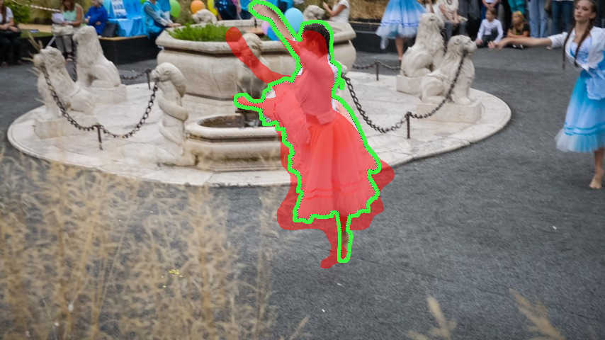
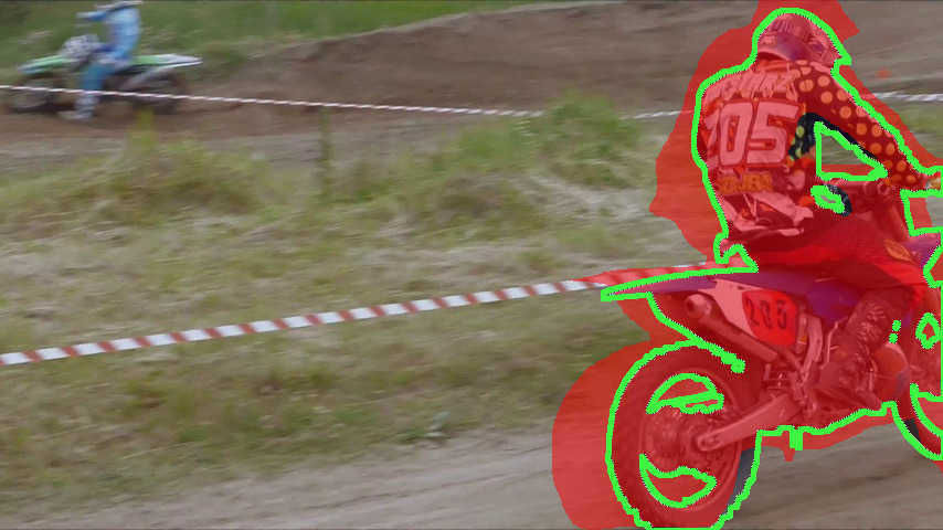
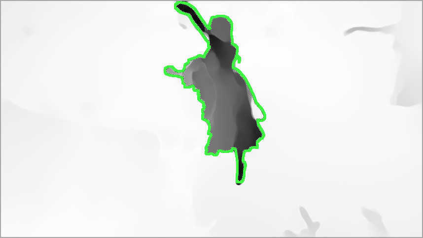
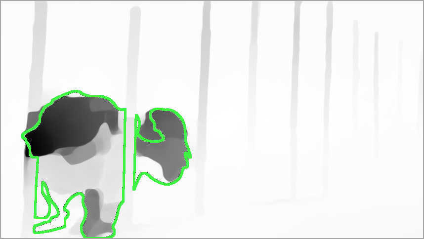
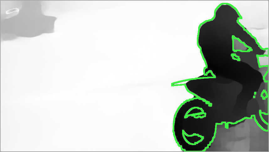
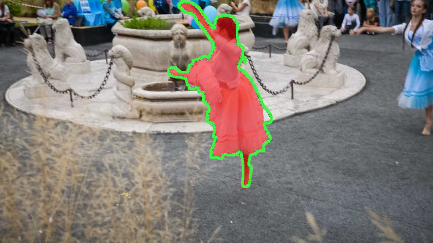
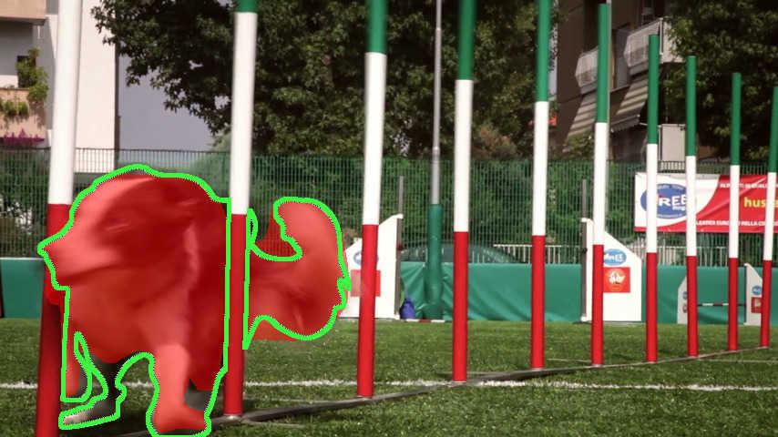
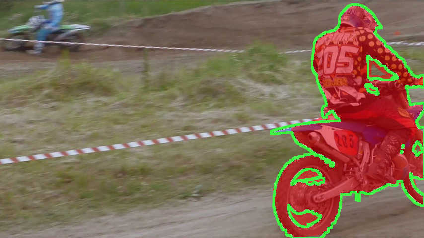
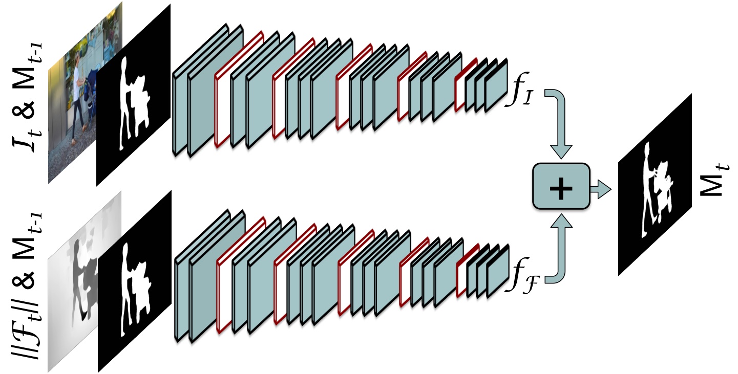
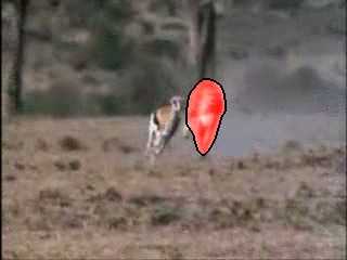
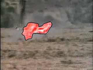
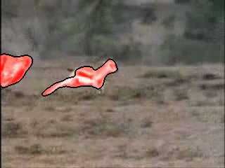
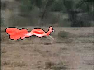
We use flow in two complementary ways. First, to obtain a better initial estimate of $M_{t}$ we warp $M_{t-1}$ using the flow $\mathcal{F}_{t}$: $M_{t}=f_{\mathcal{I}}\left(\mathcal{I}_{t},\,w(M_{t-1},\mathcal{\,F}_{t})\right)$; we call this "mask warping". Second, we use flow as a direct source of information about the mask $M_{t}$. As can be seen in Figure 2, when the object is moving relative to background, the flow magnitude $\left\|\mathcal{F}_{t}\right\|$ provides a very reasonable estimate of the mask $M_{t}$. We thus consider using a convnet specifically for mask estimation from flow: $M_{t}=f_{\mathcal{F}}\left(\left\|\mathcal{F}_{t}\right\|,\,w(M_{t-1},\mathcal{\,F}_{t})\right)$, and merge it with the image-only version by naive averaging

$$M_{t}=0.5\cdot f_{\mathcal{I}}\left(\mathcal{I}_{t},\,\ldots\right)+0.5\cdot f_{\mathcal{F}}\left(\left\|\mathcal{F}_{t}\right\|,\,\ldots\right).$$ (1)

We use the state-of-the-art optical flow estimation method FlowNet2.0 IlgCVPR17 , which itself is a convnet that computes $\mathcal{F}_{t}=h\left(\mathcal{I}_{t-1},\,\mathcal{I}_{t}\right)$ and is trained on synthetic renderings of flying objects Mayer2016Cvpr . For the optical flow magnitude computation we subtract the median motion for each frame, average the magnitude of the forward and backward flow and scale the values per-frame to $[0;255]$, bringing it to the same range as RGB channels.

The loss function is the sum of cross-entropy terms over each pixel in the output map (all pixels are equally weighted). In our experiments $f_{\mathcal{I}}$ and $f_{\mathcal{F}}$ are trained independently, via some of the modalities listed in Section 3.2. Our two streams architecture is illustrated in Figure 3a.

We also explored expanding our network to accept 5 input channels (RGB + previous mask + flow magnitude) in one stream: $M_{t}=f_{\mathcal{I+F}}\left(\mathcal{I}_{t},\,\left\|\mathcal{F}_{t}\right\|,\,w(M_{t-1},\mathcal{\,F}_{t})\right)$, but did not observe much difference in the performance compared to naive averaging, see experiments in Section 5.4.3. Our one stream architecture is illustrated in Figure 3b. One stream network is more affordable to train and allows to easily add extra input channels, e.g. providing additionally semantic information about objects.

Multiple objects

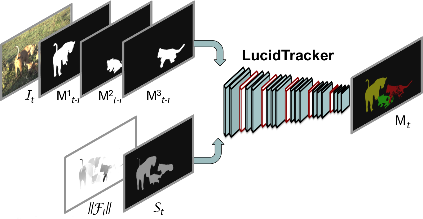
The proposed framework can easily be extended to segmenting multiple objects simultaneously. Instead of having one additional input channel for the previous frame mask we provide the mask for each object instance in a separate channel, expanding the network to accept $3+N$ input channels (RGB + $N$ object masks): $M_{t}=f_{\mathcal{I}}\left(\mathcal{I}_{t},\,w(M_{t-1}^{1},\mathcal{\,F}_{t}),{\scriptstyle\ldots},\,w(M_{t-1}^{N},\mathcal{\,F}_{t})\right)$, where $N$ is the number of objects annotated on the first frame.

For multiple object segmentation we employ a one-stream architecture for the experiments, using optical flow $\mathcal{F}$ and semantic segmentation $\mathtt{\mathcal{S}}$ as additional input channels: $M_{t}{\scriptstyle{\scriptstyle=}}f_{\mathcal{I{\scriptscriptstyle+}F{\scriptscriptstyle+}\mathcal{S}}}\left(\mathcal{I}_{t},\,\left\|\mathcal{F}_{t}\right\|,\,\mathcal{\mathcal{S}}_{t},\,w(M_{t-1}^{1},\mathcal{\,F}_{t}),{\scriptstyle\ldots},\,w(M_{t-1}^{N},\mathcal{\,F}_{t})\right)$. This allows to leverage the appearance model with semantic priors and motion information. See Figure 4 for an illustration.

The one-stream network is trained with multi-class cross entropy loss and is able to segment multiple objects simultaneously, sharing the feature computation for different instances. This allows to avoid a linear increase of the cost with the number of objects. In our preliminary results using a single architecture also pro-vides better results than segmenting multiple objects separately, one at a time; and avoids the need to design a merging strategy amongst overlapping tracks.

Semantic labels $\mathcal{S}$

To compute the pixel-level semantic labelling $\mathcal{\mathcal{S}}_{t}=h\left(\mathcal{I}_{t}\right)$ we use the state-of-the-art convnet PSPNet ZhaoSQWJ16 , trained on Pascal VOC12 Everingham15 . Pascal VOC12 annotates 20 categories, yet we want to track any type of objects. $\mathcal{\mathcal{S}}_{t}$ can also provide information about unknown category instances by describing them as a spatial mixture of known ones (e.g. a sea lion might looks like a dog torso, and the head of cat). As long as the predictions are consistent through time, $\mathcal{\mathcal{S}}_{t}$ will provide a useful cue for segmentation. Note that we only use $\mathcal{\mathcal{S}}_{t}$ for the multi-object segmentation challenge, discussed in Section 6. In the same way as for the optical flow we scale $\mathcal{\mathcal{S}}_{t}$ to bring all the channels to the same range.

We additionally experiment with ensembles of different variants, that allows to make the system more robust to the challenges inherent in videos. For our main results on the multiple object segmentation task we consider an ensemble of four models: $M_{t}{\scriptstyle{\scriptstyle=}}0.25\cdot\left(f_{\mathcal{I{\scriptscriptstyle+}F{\scriptscriptstyle+}\mathcal{S}}}+f_{\mathcal{I{\scriptscriptstyle+}F}}+f_{\mathcal{I{\scriptscriptstyle+}S}}+f_{\mathcal{I}}\right)$, where we merge the outputs of the models by naive averaging. See Section 6 for more details.

Temporal coherency

To improve the temporal coherency of the proposed video object segmentation framework we introduce an additional step into the system. Before providing as input the previous frame mask warped with the optical flow $w(M_{t-1},\mathcal{\,F}_{t})$, we look at frame $t-2$ to remove inconsistencies between the predicted masks $M_{t-1}$ and $M_{t-2}$. In particular, we split the mask $M_{t-1}$ into connected components and remove all components from $M_{t-1}$ which do not overlap with $M_{t-2}$. This way we remove possibly spurious blobs generated by our model in $M_{t-1}$. Afterwards we warp the “pruned” mask $\widetilde{{M}}_{t-1}$ with the optical flow and use $w(\widetilde{M}_{t-1},\mathcal{\,F}_{t})$ as an input to the network. This step is applied only during inference, it mitigates error propagation issues, as well as help generating more temporally coherent results.

Post-processing

As a final stage of our pipeline, we refine per-frame $t$ the generated mask $M_{t}$ using DenseCRF Kraehenbuehl2011Nips . This adjusts small image details that the network might not be able to handle. It is known by practitioners that DenseCRF is quite sensitive to its parameters and can easily worsen results. We will use our lucid dreams to handle per-dataset CRF-tuning too, see Section 3.2.

We refer to our full $f_{\mathcal{I{\scriptscriptstyle+}F}}$ system as $\mathtt{LucidTracker}$, and as $\mathtt{LucidTracker^{-}}$ when no temporal coherency or post-processing steps are used. The usage of $S_{t}$ or model ensemble will be explicitly stated.

Figure 4: Extension of LucidTracker to multiple objects. The previous frame mask for each object is provided in a separate channel. We additionally explore using optical flow $\mathcal{F}$ and semantic segmentation $\mathtt{\mathcal{S}}$ as additional inputs. See Section 3.1.

3.2 Training modalities

Multiple modalities are available to train a tracker. Training-free approaches (e.g. BVS Maerki2016Cvpr , SVT Wang2017ArxivSTV ) are fully hand-crafted systems with hand-tuned parameters, and thus do not require training data. They can be used as-is over different datasets. Supervised methods can also be trained to generate a dataset-agnostic model that can be applied over different datasets. Instead of using a fixed model for all cases, it is also possible to obtain specialized per-dataset models, either via self-supervision Wang2015IccvUnsupervised ; Pathak2016Arxiv ; Yu2016ArxivFlow ; Zhu2017ArxivFlow or by using the first frame annotation of each video in the dataset as training/tuning set. Finally, inspired by traditional box tracking techniques, we also consider adapting the model weights to the specific video at hand, thus obtaining per-video models. Section 5 reports new results over these four training modalities (training-free, dataset-agnostic, per-dataset, and per-video).

Our $\mathtt{LucidTracker}$ obtains best results when first pre-trained on ImageNet, then trained per-dataset using all data from first frame annotations together, and finally fine-tuned per-video for each evaluated sequence. The post-processing DenseCRF stage is automatically tuned per-dataset. The experimental section 5 details the effect of these training stages. Surprisingly, we can obtain reasonable performance even when training from only a single annotated frame (without ImageNet pre-training, i.e. zero pre-training); this results goes against the intuition that convnets require large training data to provide good results.

Unless otherwise stated, we fine-tune per-video models relying solely on the first frame $\mathcal{I}_{0}$ and its annotation $M_{0}$. This is in contrast to traditional techniques Henriques2012Eccv ; breitenstein2009robust ; Hadfield14d which would update the appearance model at each frame $\mathcal{I}_{t}$.

4 Lucid data dreaming

To train the function $f$ one would think of using ground truth data for $M_{t-1}$ and $M_{t}$ (like Bertinetto2016Arxiv ; Caelles2017Cvpr ; Held2016Eccv ), however such data is expensive to annotate and rare. Caelles2017Cvpr thus trains on a set of $30$ videos ($\sim\negmedspace 2k$ frames) and requires the model to transfer across multiple tests sets. Khoreva2017CvprMaskTrack side-steps the need for consecutive frames by generating synthetic masks $M_{t-1}$ from a saliency dataset of $\sim\negmedspace 10k$ images with their corresponding mask $M_{t}$ . We propose a new data generation strategy to reach better results using only $\sim\negmedspace 100$ individual training frames.

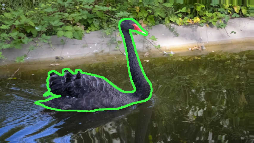
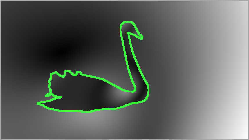
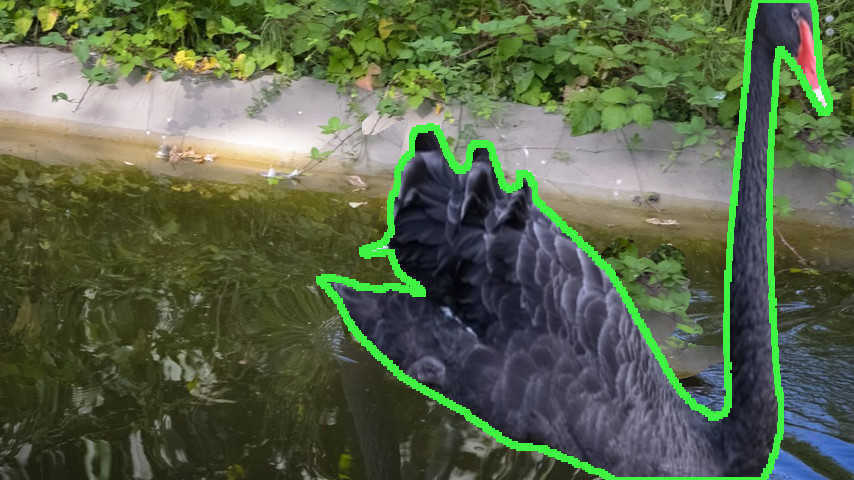
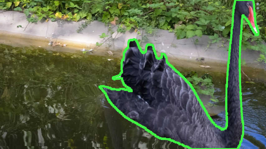
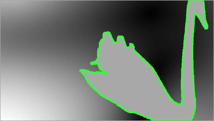
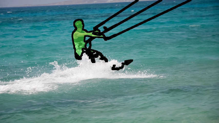
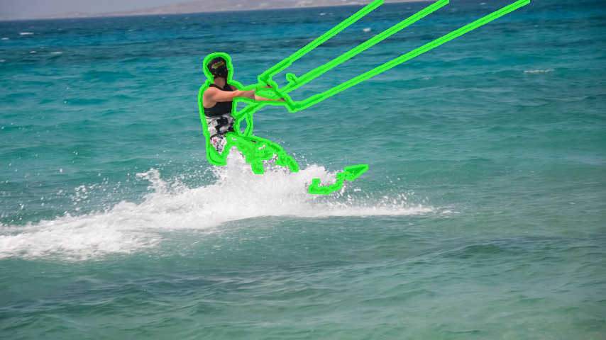
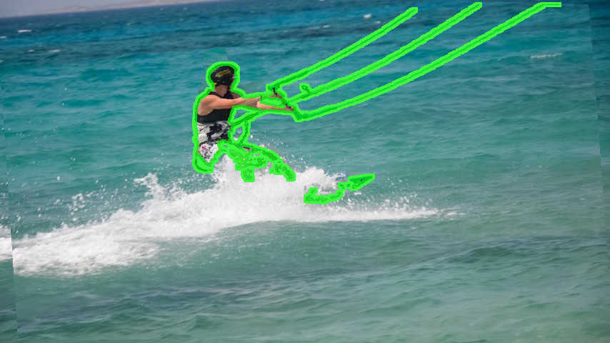
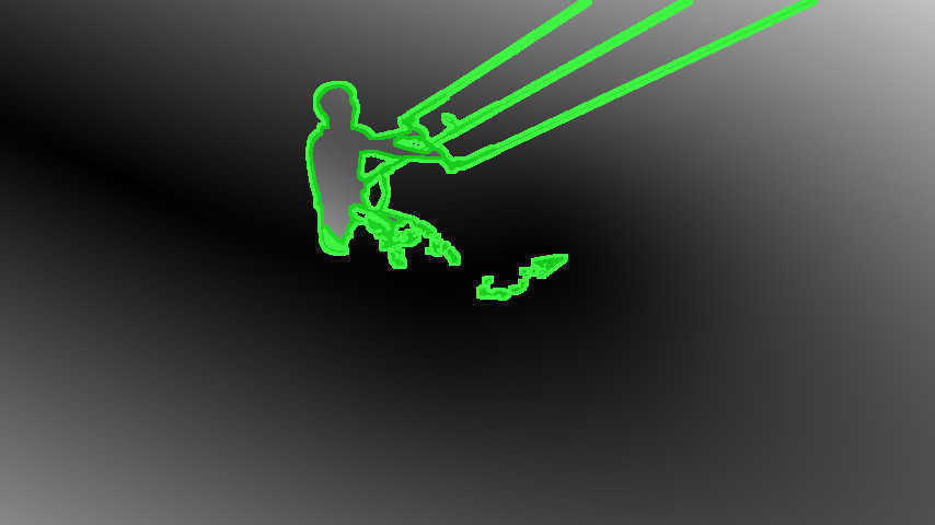
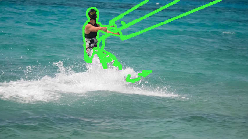
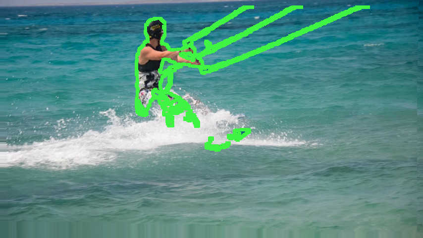
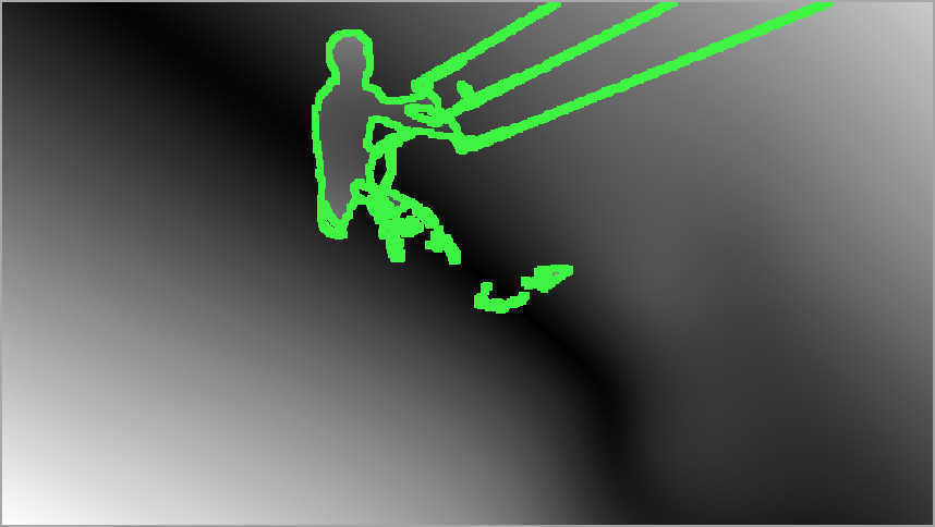
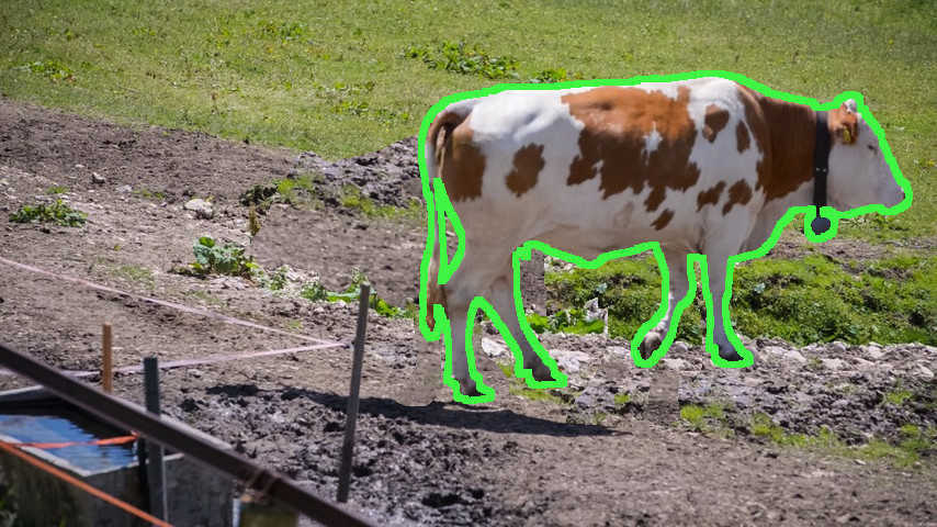
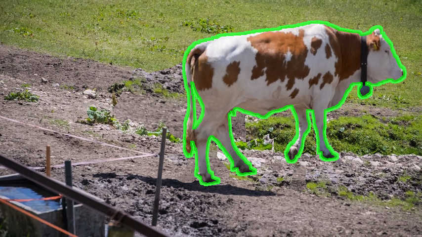
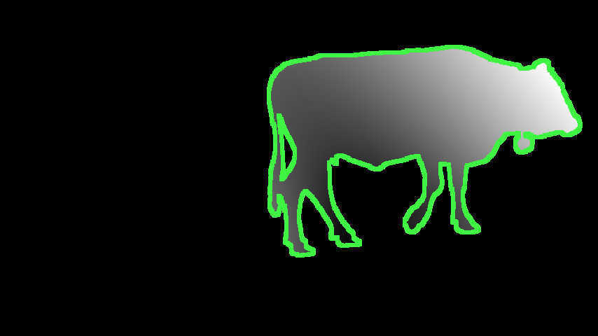
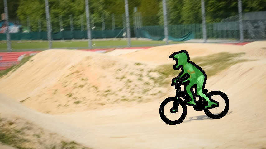
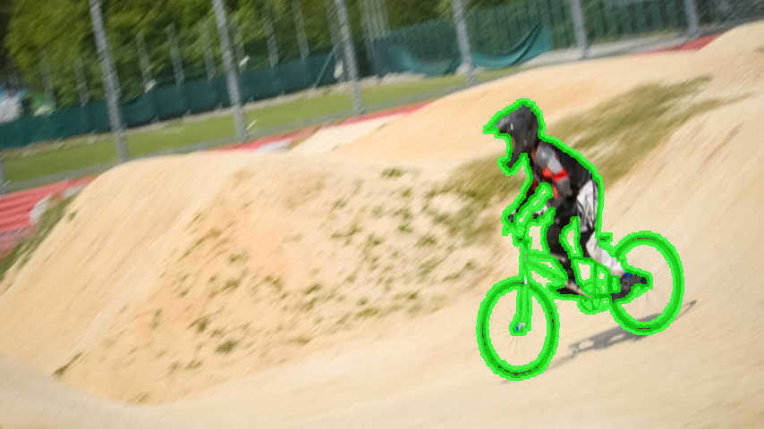
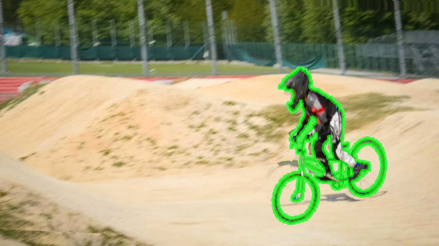
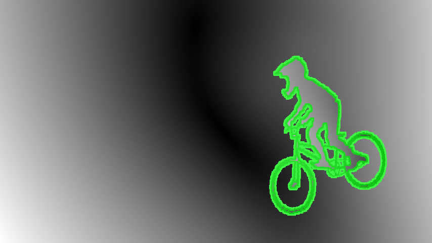
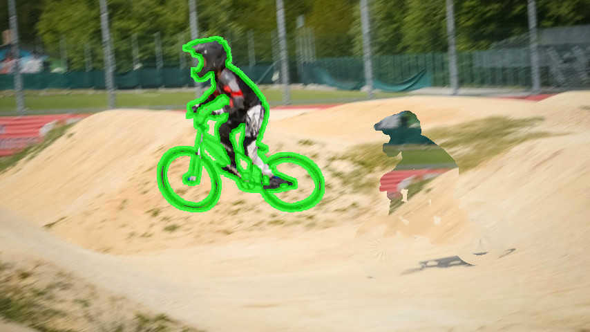
Ideally training data should be as similar as possible to the test data, even subtle differences may affect quality (e.g. training on static images for testing on videos under-performs Tang_NIPS2012 ). To ensure our training data is in-domain, we propose to generate it by synthesizing samples from the provided annotated frame (first frame) in each target video. This is akin to “lucid dreaming” as we intentionally “dream” the desired data by creating sample images that are plausible hypothetical future frames of the video. The outcome of this process is a large set of frame pairs in the target domain ($2.5k$ pairs per annotation) with known optical flow and mask annotations, see Figure 5.

Synthesis process

The target domain for a tracker is the set of future frames of the given video. Traditional data augmentation via small image perturbation is insufficient to cover the expect variations across time, thus a task specific strategy is needed. Across the video the tracked object might change in illumination, deform, translate, be occluded, show different point of views, and evolve on top of a dynamic background. All of these aspects should be captured when synthesizing future frames. We achieve this by cutting-out the foreground object, in-painting the background, perturbing both foreground and background, and finally recomposing the scene. This process is applied twice with randomly sampled transformation parameters, resulting in a pair of frames ($\mathcal{I}_{\tau-1},\,\mathcal{I}_{\tau}$) with known pixel-level ground-truth mask annotations ($M_{\tau-1},\,M_{\tau}$), optical flow $\mathcal{F}_{\tau}$, and occlusion regions. The object position in $\mathcal{I}_{\tau}$ is uniformly sampled, but the changes between $\mathcal{I}_{\tau-1},\,\mathcal{I}_{\tau}$ are kept small to mimic the usual evolution between consecutive frames.
In more details, starting from an annotated image:
1. Illumination changes: we globally modify the image by randomly altering saturation S and value V (from HSV colour space) via $x^{\prime}=a\cdot x^{b}+c$, where $a\in 1\pm 0.05$, $b\in 1\pm 0.3$, and $c\in\pm 0.07$.
2. Fg/Bg split: the foreground object is removed from the image $\mathcal{I}_{0}$ and a background image is created by inpainting the cut-out area Criminisi2004 .
3. Object motion: we simulate motion and shape deformations by applying global translation as well as affine and non-rigid deformations to the foreground object. For $\mathcal{I}_{\tau-1}$ the object is placed at any location within the image with a uniform distribution, and in $\mathcal{I}_{\tau}$ with a translation of $\pm 10\%$ of the object size relative to $\tau-1$. In both frames we apply random rotation $\pm 30^{\circ}$, scaling $\pm 15\%$ and thin-plate splines deformations Bookstein1989Pami of $\pm 10\%$ of the object size.
4. Camera motion: We additionally transform the background using affine deformations to simulate camera view changes. We apply here random translation, rotation, and scaling within the same ranges as for the foreground object.
5. Fg/Bg merge: finally ($\mathcal{I}_{\tau-1},\,\mathcal{I}_{\tau}$) are composed by blending the perturbed foreground with the perturbed background using Poisson matting Sun2004 . Using the known transformation parameters we also synthesize ground-truth pixel-level mask annotations ($M_{\tau-1},\,M_{\tau}$) and optical flow $\mathcal{F}_{\tau}$.
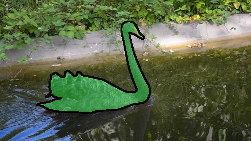
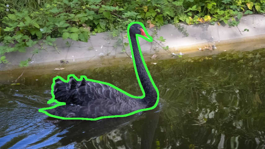
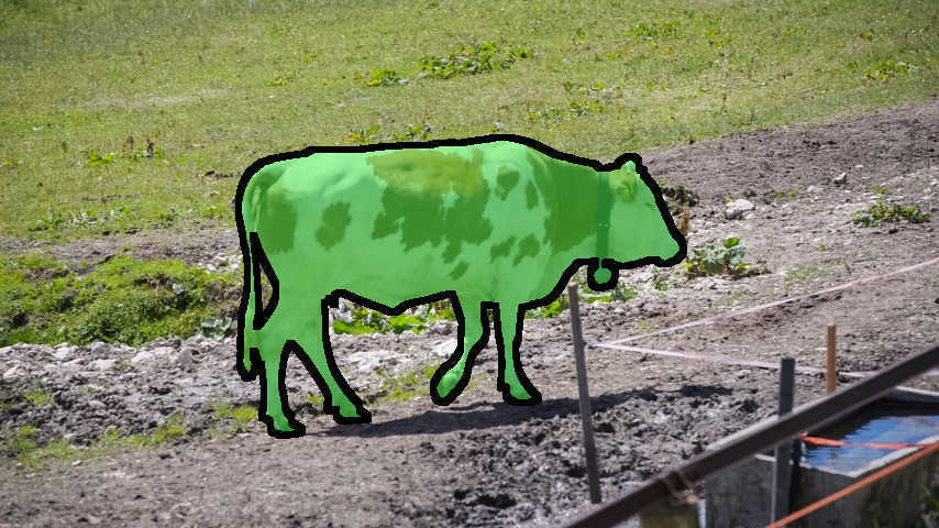
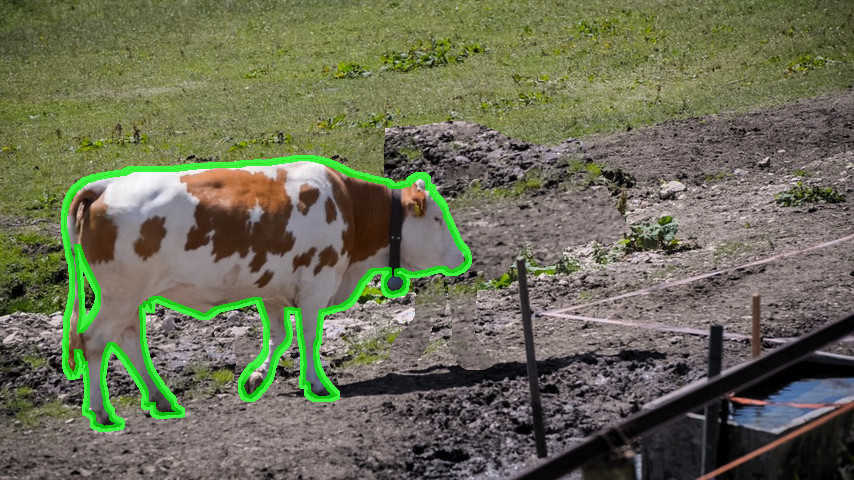
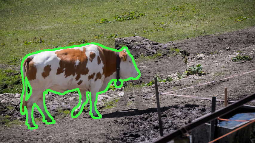
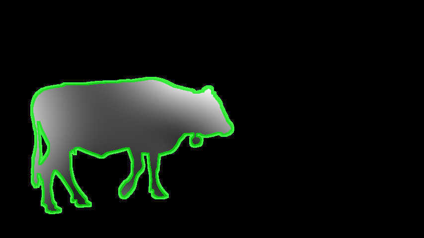
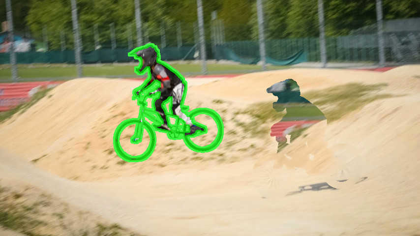
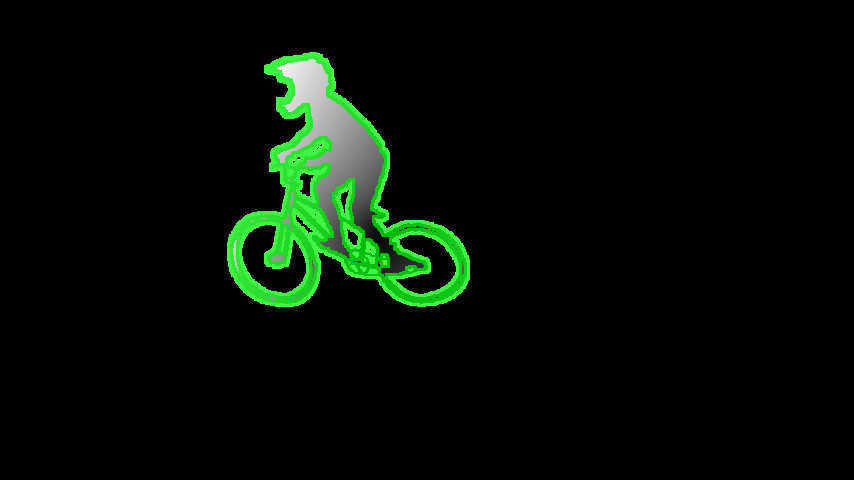
Figure 5 shows example results. Albeit our approach does not capture appearance changes due to point of view, occlusions, nor shadows, we see that already this rough modelling is effective to train our segmentation models.

blackswan
kite-surf
cows
bmx-bumps
Original image $\mathcal{I}_{0}$ and mask annotation $M_{0}$			Generated image $\mathcal{I}_{\tau-1}$	Generated image $\mathcal{I}_{\tau}$	Generated flow magnitude $\left\|\mathcal{F}_{\tau}\right\|$

Figure 5: Lucid data dreaming examples. From one annotated frame we generate pairs of images ($\mathcal{I}_{\tau-1},\,\mathcal{I}_{\tau}$) that are plausible future video frames, with known optical flow ($\mathcal{F}_{\tau}$) and masks (green boundaries). Note the inpainted background and foreground/background deformations.

The number of synthesized images can be arbitrarily large. We generate $2.5k$ pairs per annotated video frame. This training data is, by design, in-domain with regard of the target video. The experimental section 5 shows that this strategy is more effective than using thousands of manually annotated images from close-by domains.

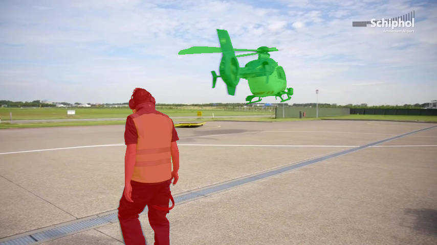
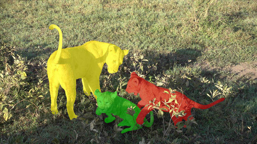
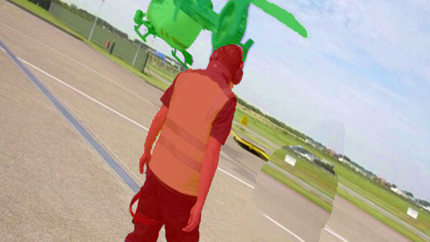
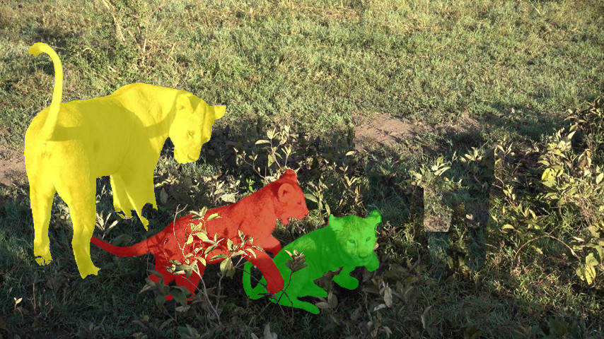
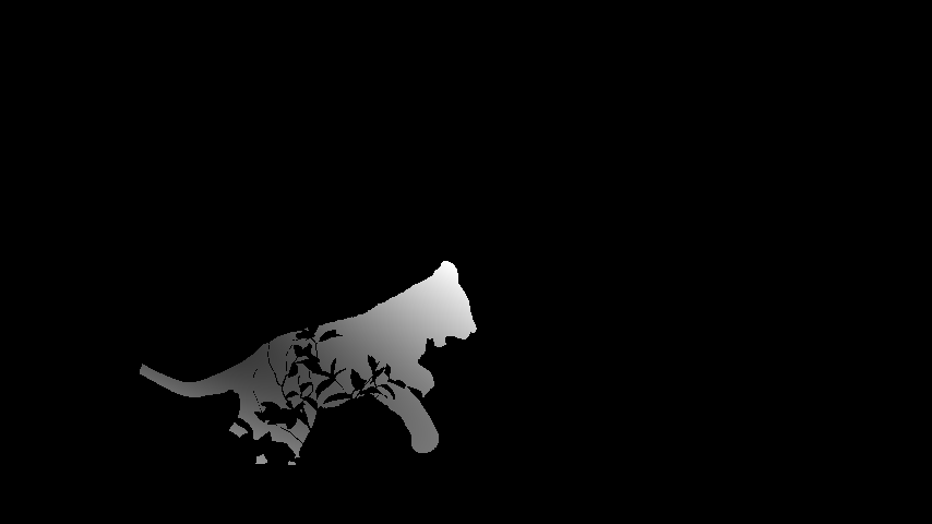
The same strategy for data synthesis can be employed for multiple object segmentation task. Instead of manipulating a single object we handle multiple ones at the same time, applying independent transformations to each of them. We model occlusion between objects by adding a random depth ordering obtaining both partial and full occlusions in the training set. Including occlusions in the lucid dreams allows to better handle plausible interactions of objects in the future frames. See Figure 6 for examples of the generated data.

(a) Original image $\mathcal{I}_{0}$ and mask annotation $M_{0}$

(b) Generated image $\mathcal{I}_{\tau}$ and mask $M_{\tau}$

(c) Generated flow magnitude $\left\|\mathcal{F}_{\tau}\right\|$

Figure 6: Lucid data dreaming examples with multiple objects. From one annotated frame we generate a plausible future video frame ($\mathcal{I}_{\tau}$), with known optical flow ($\mathcal{F}_{\tau}$) and mask ($M_{\tau}$).

5 Single object segmentation results

We present here a detailed empirical evaluation on three different datasets for the single object segmentation task: given a first frame labelled with the foreground object mask, the goal is to find the corresponding object pixels in future frames. (Section 6 will discuss the multiple objects case.)

5.1 Experimental setup

Datasets

We evaluate our method on three video object segmentation datasets: $\text{DAVIS}_{\text{16}}$ Perazzi2016Cvpr , YouTubeObjects Prest2012Cvpr ; Jain2014Eccv , and $\text{SegTrack}_{\text{v2}}$ Li2013Iccv . The goal is to track an object through all video frames given an object mask in the first frame. These three datasets provide diverse challenges with a mix of high and low resolution web videos, single or multiple salient objects per video, videos with flocks of similar looking instances, longer ($\sim\negmedspace 400$ frames) and shorter ($\sim\negmedspace 10$ frames) sequences, as well as the usual video segmentation challenges such as occlusion, fast motion, illumination, view point changes, elastic deformation, etc.

The $\text{DAVIS}_{\text{16}}$ Perazzi2016Cvpr video segmentation benchmark consists of 50 full-HD videos of diverse object categories with all frames annotated with pixel-level accuracy, where one single or two connected moving objects are separated from the background. The number of frames in each video varies from 25 to 104.

YouTubeObjects Prest2012Cvpr ; Jain2014Eccv includes web videos from 10 object categories. We use the subset of 126 video sequences with mask annotations provided by Jain2014Eccv for evaluation, where one single object or a group of objects of the same category are separated from the background. In contrast to $\text{DAVIS}_{\text{16}}$ these videos have a mix of static and moving objects. The number of frames in each video ranges from 2 to 401.

$\text{SegTrack}_{\text{v2}}$Li2013Iccv consists of 14 videos with multiple object annotations for each frame. For videos with multiple objects each object is treated as a separate problem, resulting in 24 sequences. The length of each video varies from 21 to 279 frames. The images in this dataset have low resolution and some compression artefacts, making it hard to track the object based on its appearance.

The main experimental work is done on $\text{DAVIS}_{\text{16}}$, since it is the largest densely annotated dataset out of the three, and provides high quality/high resolution data. The videos for this dataset were chosen to represent diverse challenges, making it a good experimental playground.

We additionally report on the two other datasets as complementary test set results.

Evaluation metric

To measure the accuracy of video object segmentation we use the mean intersection-over-union overlap (mIoU) between the per-frame ground truth object mask and the predicted segmentation, averaged across all video sequences. We have noticed disparate evaluation procedures used in previous work, and we report here a unified evaluation across datasets. When possible, we re-evaluated certain methods using results provided by their authors. For all three datasets we follow the $\text{DAVIS}_{\text{16}}$ evaluation protocol, excluding the first frame from evaluation and using all other frames from the video sequences, independent of object presence in the frame.

$\text{DAVIS}_{\text{16}}$
YouTubeObjects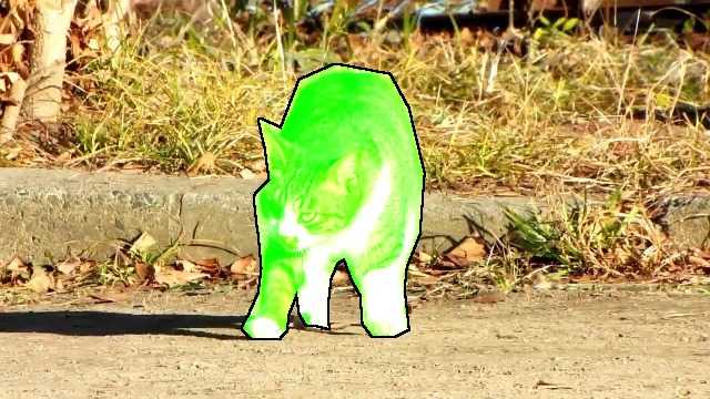
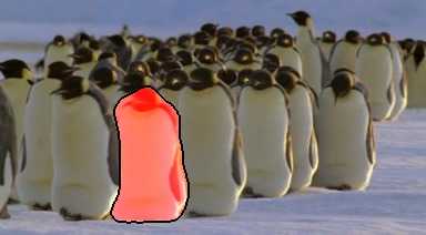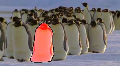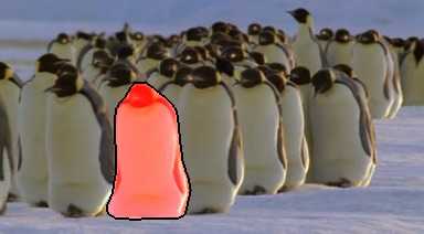$\text{SegTrack}_{\text{v2}}$
	1st frame, GT segment	$20\%$	$40\%$	$60\%$	$80\%$	$100\%$

Figure 7: LucidTracker single object segmentation qualitative results. Frames sampled along the video duration (e.g. $50\%$: video middle point). Our model is robust to various challenges, such as view changes, fast motion, shape deformations, and out-of-view scenarios.

Training details

For training all the models we use SGD with mini-batches of $10$ images and a fixed learning policy with initial learning rate of $10^{-3}$. The momentum and weight decay are set to $0.9$ and $5\cdot 10^{-4}$ , respectively.

Models using pre-training are initialized with weights trained for image classification on ImageNet Simonyan2015Iclr . We then train per-dataset for 40k iterations with the RGB+Mask branch $f_{\mathcal{I}}$ and for 20k iterations for the Flow+Mask $f_{\mathcal{F}}$ branch. When using a single stream architecture (Section 5.4.3), we use 40k iterations.

Models without ImageNet pre-training are initialized using the Xavier (also known as Glorot) random weight initialization strategy Glorot10understandingthe . (The weights are initialized as random draws from a truncated normal distribution with zero mean and standard deviation calculated based on the number of input and output units in the weight tensor, see Glorot10understandingthe for details). The per-dataset training needs to be longer, using 100k iterations for the $f_{\mathcal{I}}$ branch and 40k iterations for the $f_{\mathcal{F}}$ branch.

For per-video fine-tuning 2k iterations are used for $f_{\mathcal{I}}$. To keep computing cost lower, the $f_{\mathcal{F}}$ branch is kept fix across videos.

All training parameters are chosen based on $\text{DAVIS}_{\text{16}}$ results. We use identical parameters on YouTubeObjects and $\text{SegTrack}_{\text{v2}}$, showing the generalization of our approach.

It takes ~3.5h to obtain each per-video model, including data generation, per-dataset training, per-video fine-tuning and per-dataset grid search of CRF parameters (averaged over $\text{DAVIS}_{\text{16}}$, amortising the per-dataset training time over all videos). At test time our LucidTracker runs at ~5s per frame, including the optical flow estimation with FlowNet2.0 IlgCVPR17 (~0.5s) and CRF post-processing Kraehenbuehl2011Nips (~2s).

5.2 Key results

Table 1 presents our main result and compares it to previous work. Our full system, $\mathtt{LucidTracker}$, provides the best video segmentation quality across three datasets while being trained on each dataset using only one frame per video ($50$ frames for $\text{DAVIS}_{\text{16}}$, $126$ for YouTubeObjects, $24$ for $\text{SegTrack}_{\text{v2}}$), which is $20\times\negmedspace\sim\negmedspace 1000\times$ less than the top competing methods. Ours is the first method to reach $>75\ \text{mIoU}$ on all three datasets.

Oracles and baselines

Grabcut oracle computes grabcut Rother2004SiggraphGrabcut using the ground truth bounding boxes (box oracle). This oracle indicates that on the considered datasets separating foreground from background is not easy, even if a perfect box-level tracker was available.
We provide three additional baselines. “Saliency” corresponds to using the generic (training-free) saliency method EQCut Aytekin2015IcipEQCut over the RGB image $\mathcal{I}_{t}$. “Flow saliency” does the same, but over the optical flow magnitude $\left\|\mathcal{F}_{t}\right\|$. Results indicate that the objects being tracked are not particularly salient in the image. On $\text{DAVIS}_{\text{16}}$ motion saliency is a strong signal but not on the other two datasets. Saliency methods ignore the first frame annotation provided for the task. We also consider the “Mask warping” baseline which uses optical flow to propagate the mask estimate from $t$ to $t+1$ via simple warping $M_{t}=w(M_{t-1},\mathcal{\,F}_{t})$. The bad results of this baseline indicate that the high quality flow IlgCVPR17 that we use is by itself insufficient to solve the video object segmentation task, and that indeed our proposed convnet does the heavy lifting.

The large fluctuation of the relative baseline results across the three datasets empirically confirms that each of them presents unique challenges.

	Method	# training	Flow	Dataset, mIoU
		images	$\mathcal{F}$	$\text{DAVIS}_{\text{16}}$	YoutbObjs	$\mbox{SegTrck}_{\mbox{v2}}$
	Box oracle Khoreva2017CvprMaskTrack	0	✗	45.1	55.3	56.1
	Grabcut oracle Khoreva2017CvprMaskTrack	0	✗	67.3	67.6	74.2
Ignores 1st frame annotation	Saliency	0	✗	32.7	40.7	22.2
	NLC Faktor2014Bmvc	0	✓	64.1	-	-
	TRS Xiao2016Cvpr	0	✓	-	-	69.1
	MP-Net Tokmakov2016Arxiv	~22.5k	✓	69.7	-	-
	Flow saliency	0	✓	70.7	36.3	35.9
	FusionSeg Jain2017ArxivFusionSeg	~95k	✓	71.5	67.9	-
	LVO TokmakovAS17	~35k	✓	75.9	-	57.3
	PDB Song_2018_ECCV	~18k	✗	77.2	-	-
Uses 1st frame annotation	Mask warping	0	✓	32.1	43.2	42.0
	FCP Perazzi2015Iccv	0	✓	63.1	-	-
	BVS Maerki2016Cvpr	0	✗	66.5	59.7	58.4
	N15 Nagaraja2015Iccv	0	✓	-	-	69.6
	ObjFlow Tsai2016Cvpr	0	✓	71.1	70.1	67.5
	STV Wang2017ArxivSTV	0	✓	73.6	-	-
	VPN Jampani2016Arxiv	~2.3k	✗	75.0	-	-
	OSVOS Caelles2017Cvpr	~2.3k	✗	79.8	72.5	65.4
	MaskTrack Khoreva2017CvprMaskTrack	~11k	✓	80.3	72.6	70.3
	PReMVOS Luiten18ACCV	~145k	✓	84.9	-	-
	OnAVOS Voigtlaender2017OnlineAO	~120k	✗	86.1	-	-
	VideoGCRF Chandra2018DeepSR	~120k	✗	86.5	-	-
	LucidTracker	24~126	✓	86.6	77.3	78.0

Table 1: Comparison of video object segmentation results across three datasets. Numbers in italic are reported on subsets of $\text{DAVIS}_{\text{16}}$. Our LucidTracker consistently improves over previous results, see Section 5.2.

Comparison

Compared to flow propagation methods such as BVS, N15, ObjFlow, and STV, we obtain better results because we build per-video a stronger appearance model of the tracked object (embodied in the fine-tuned model). Compared to convnet learning methods such as VPN, OSVOS, MaskTrack, OnAVOS, we require significantly less training data, yet obtain better results.

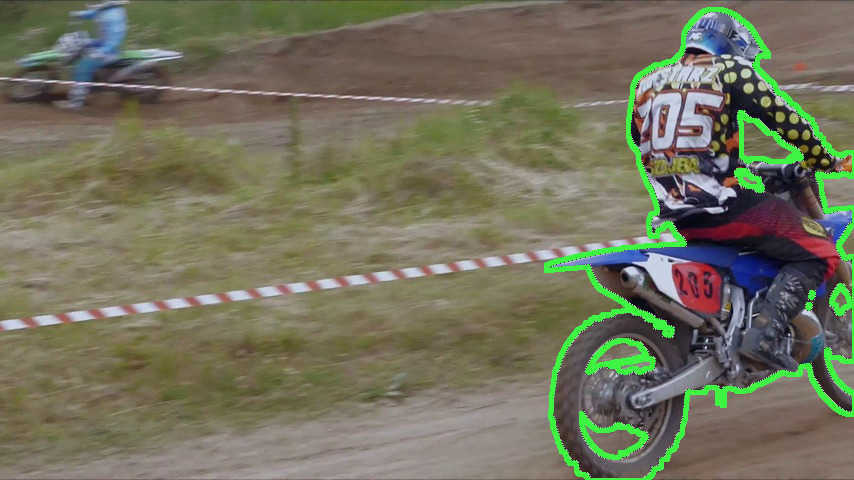
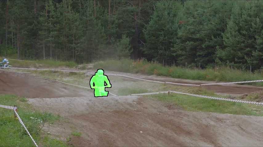
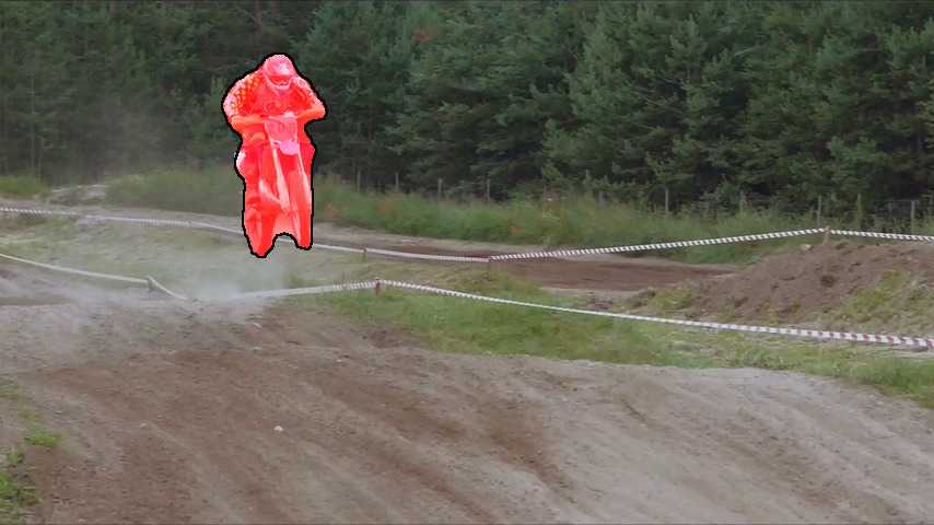
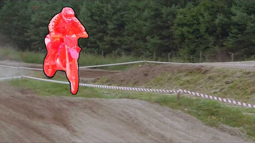
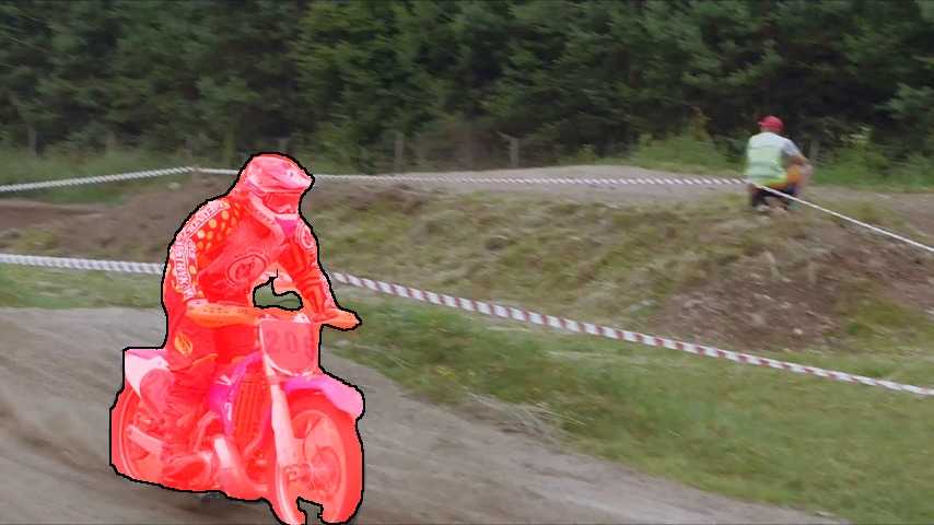
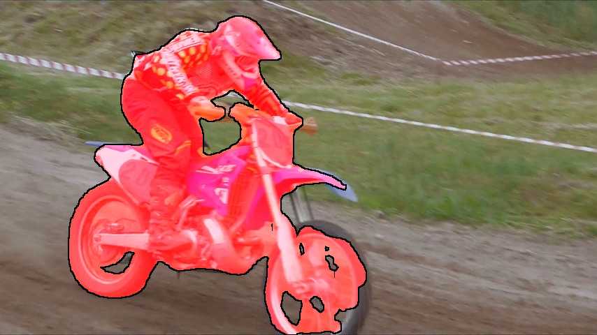
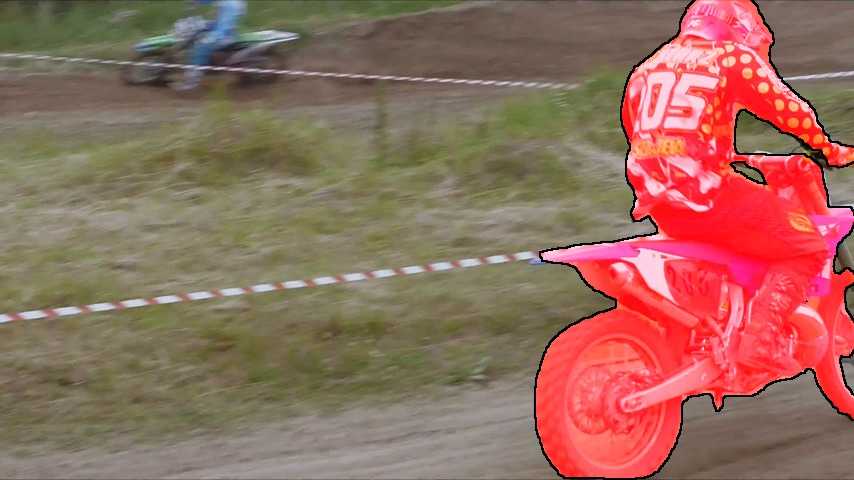
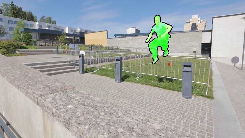
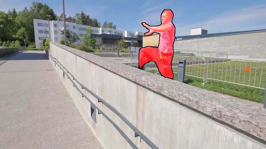
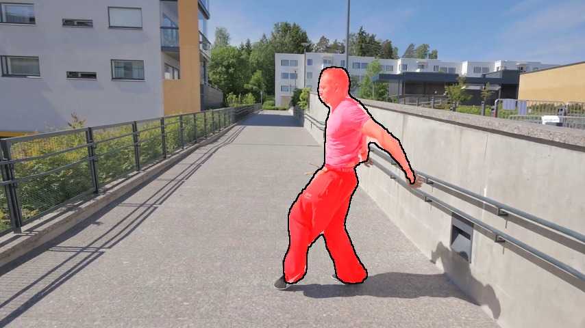
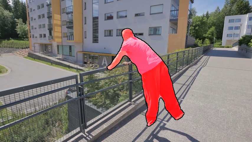
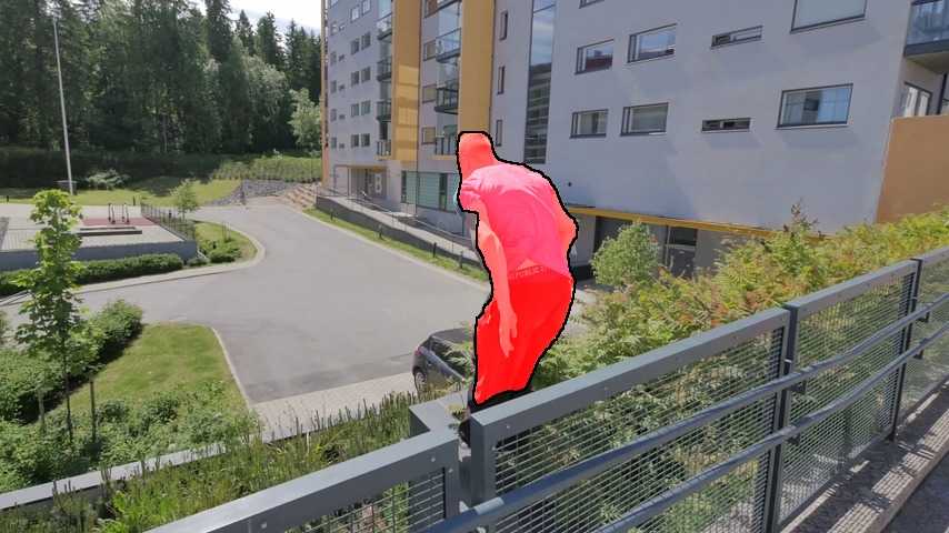
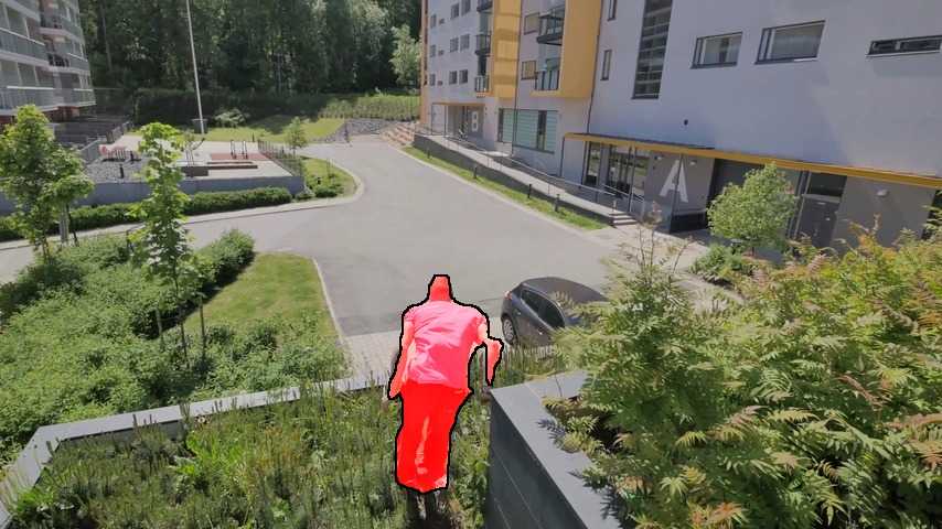
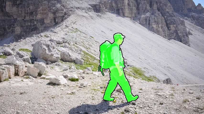
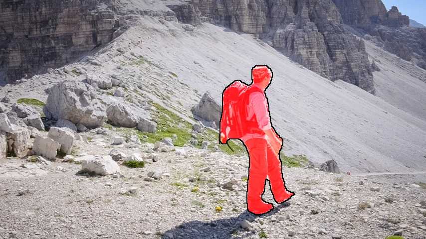
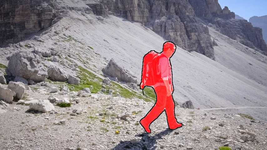
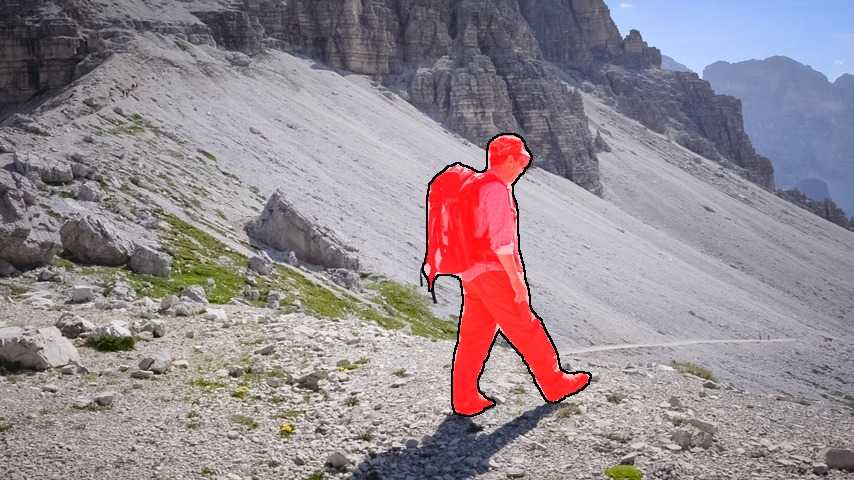
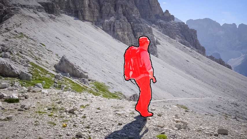
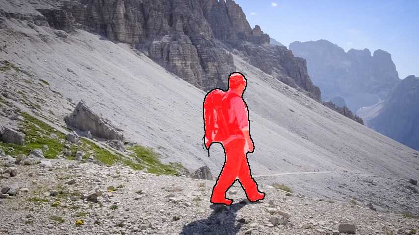
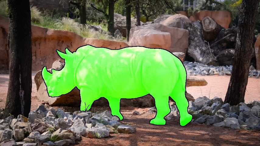
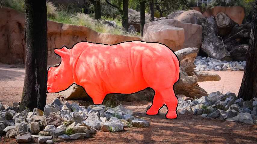
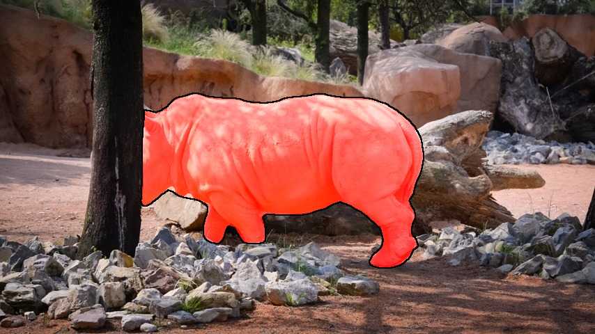
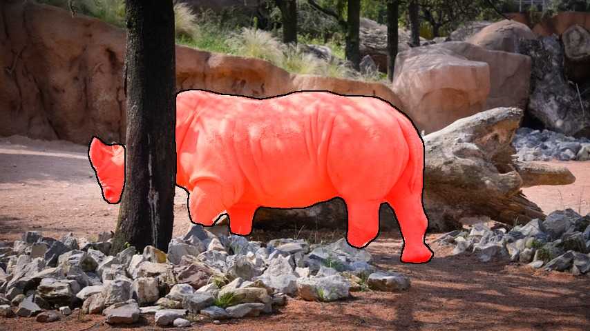
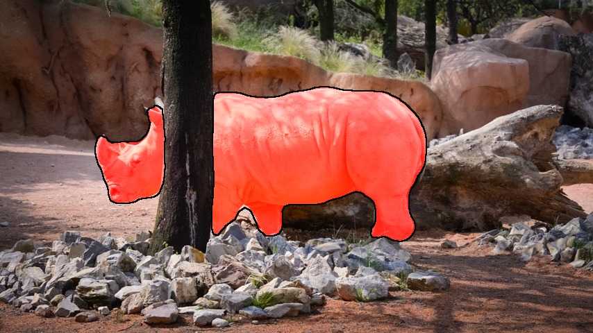
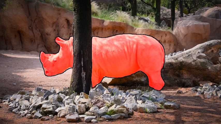
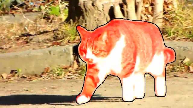
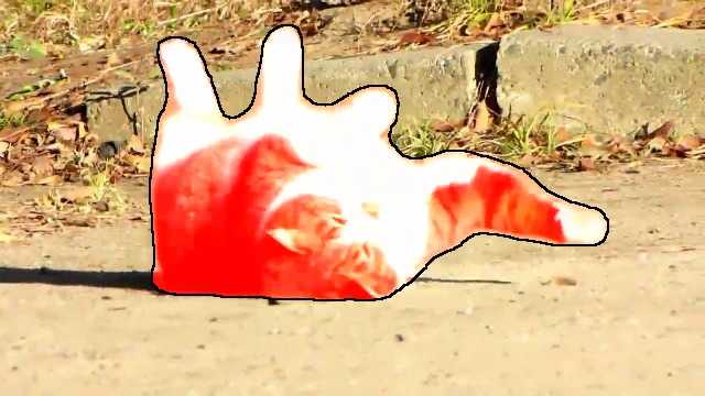
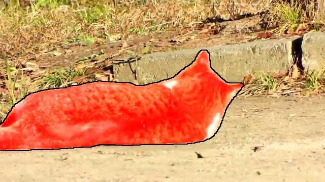
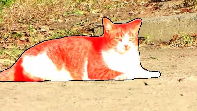
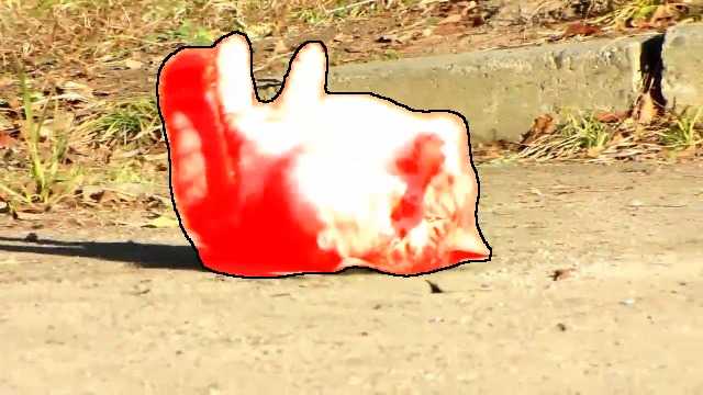
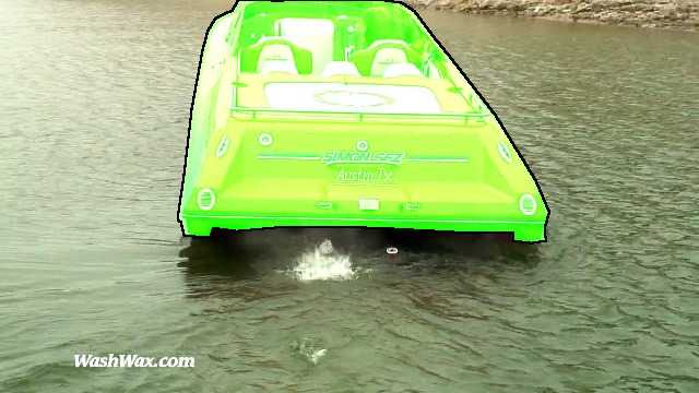
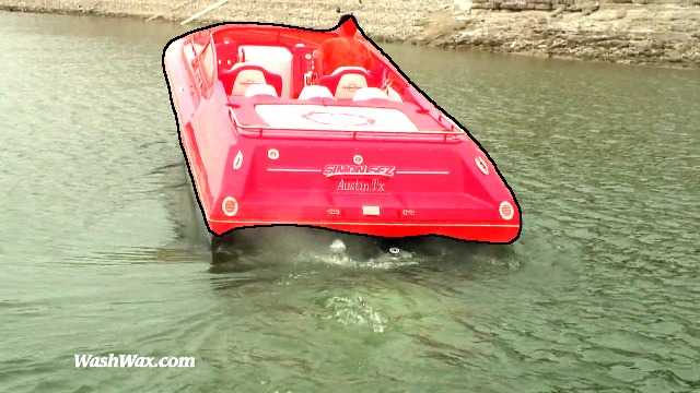
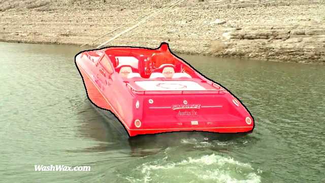
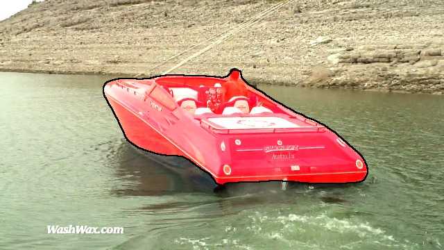
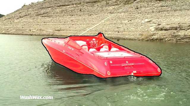
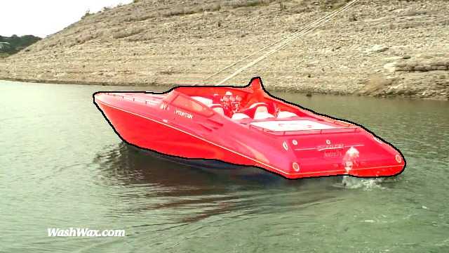
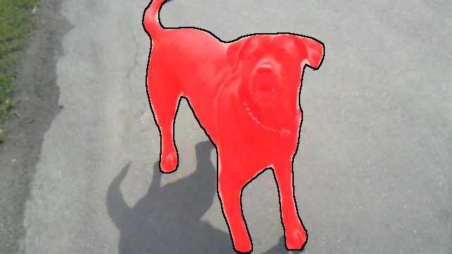
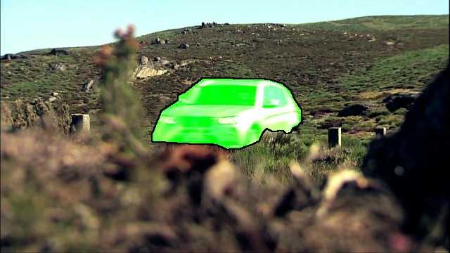
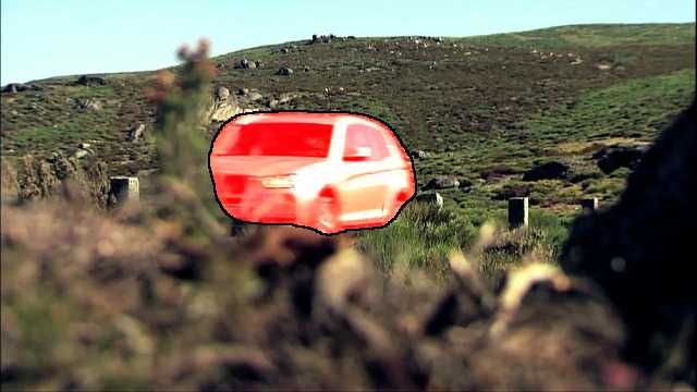
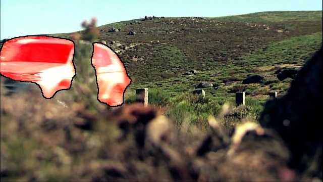
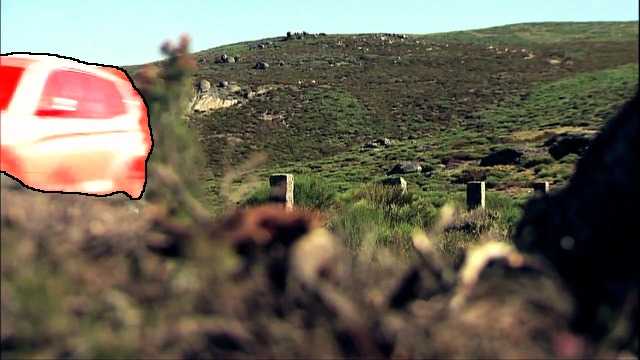
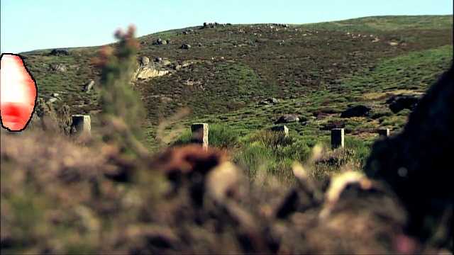
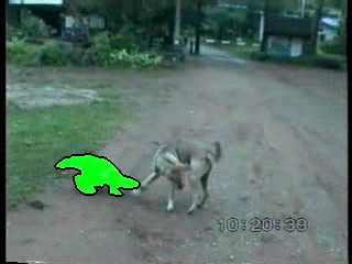
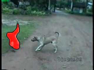
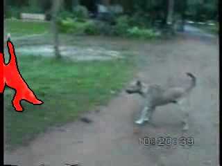
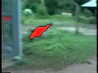
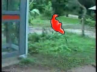
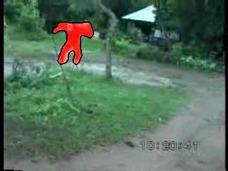
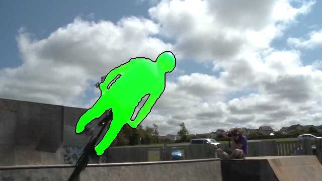
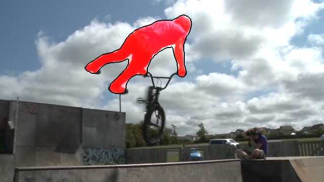
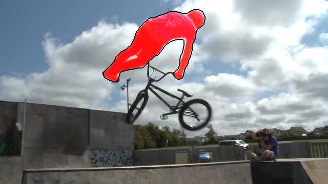
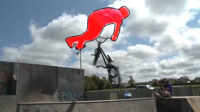
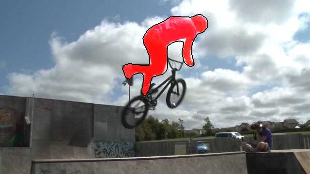
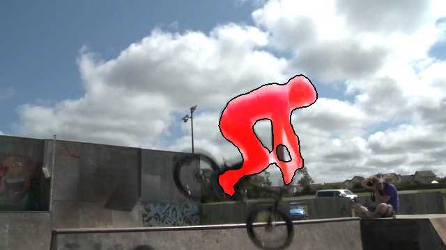
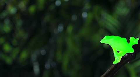
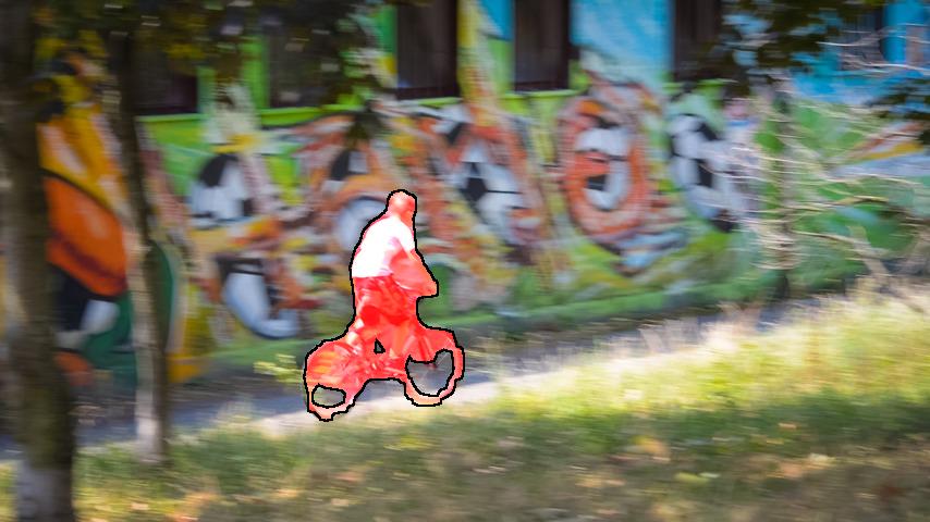
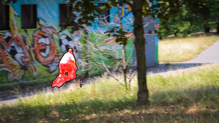
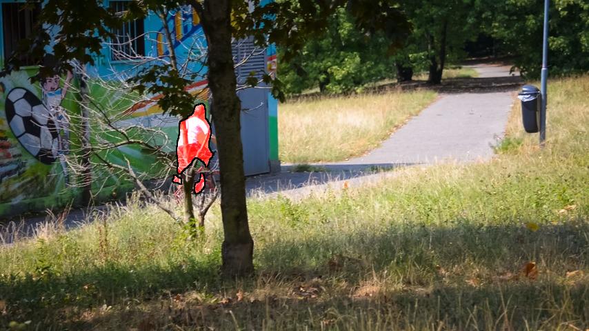
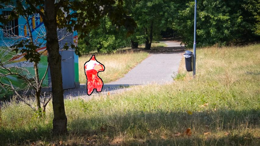
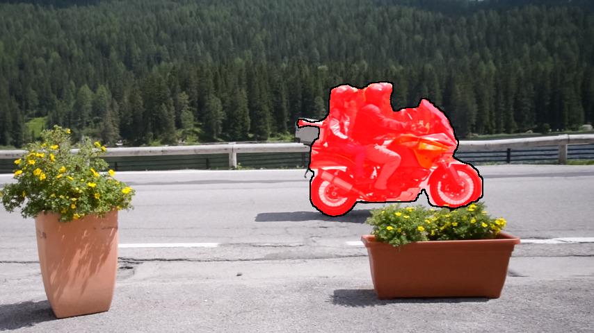
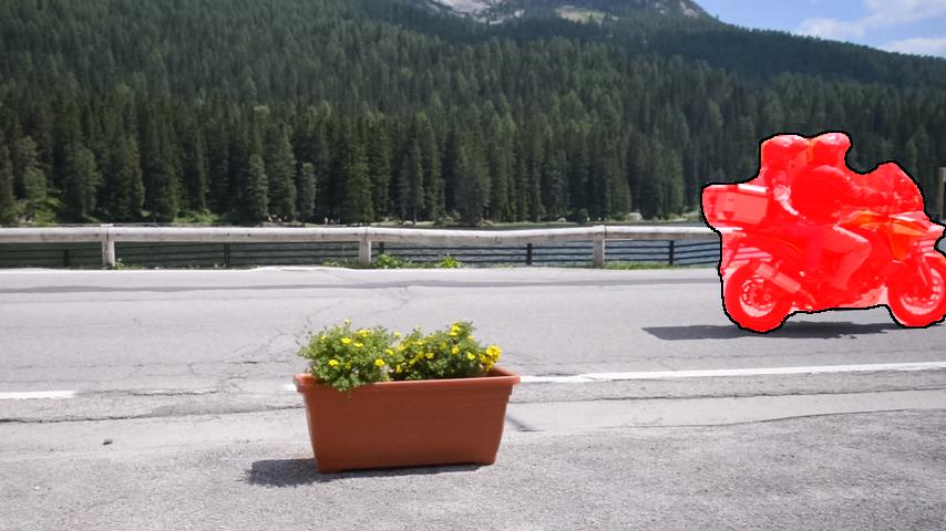
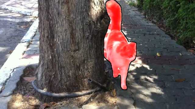
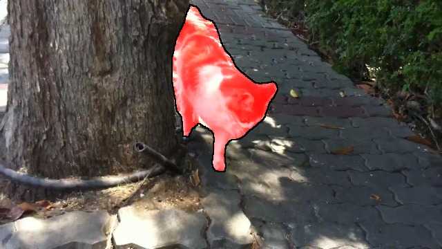
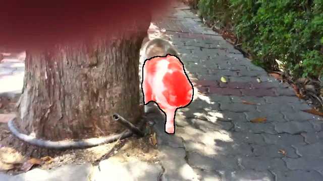
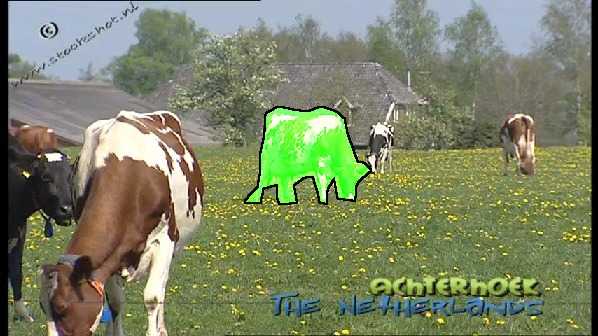
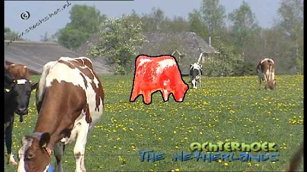
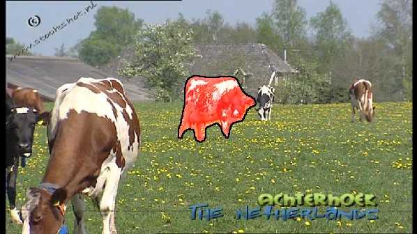
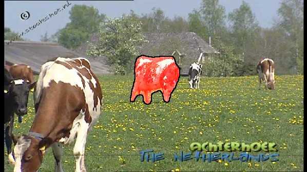
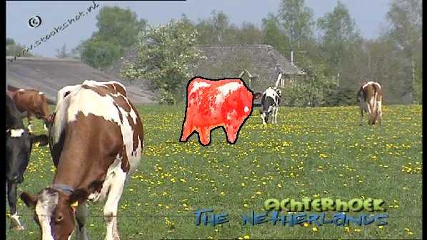
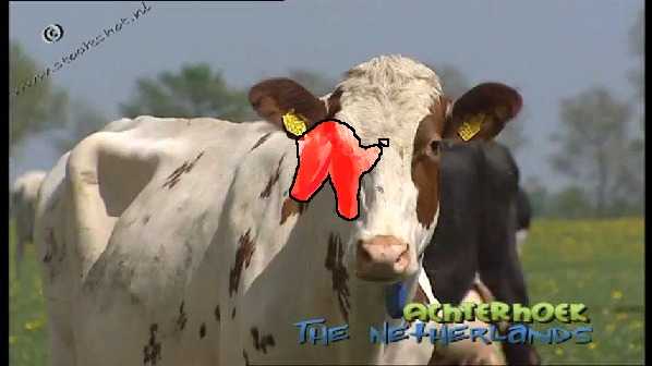
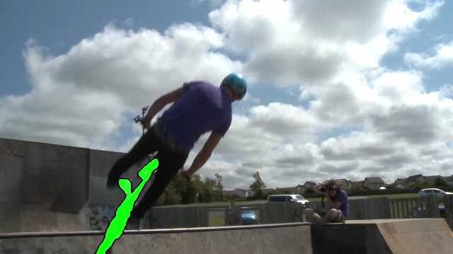
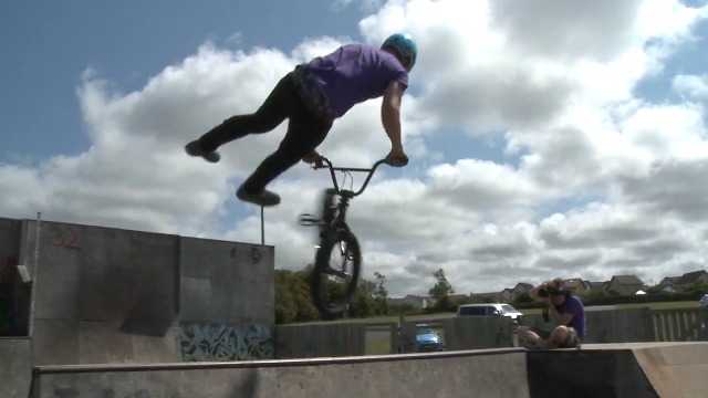
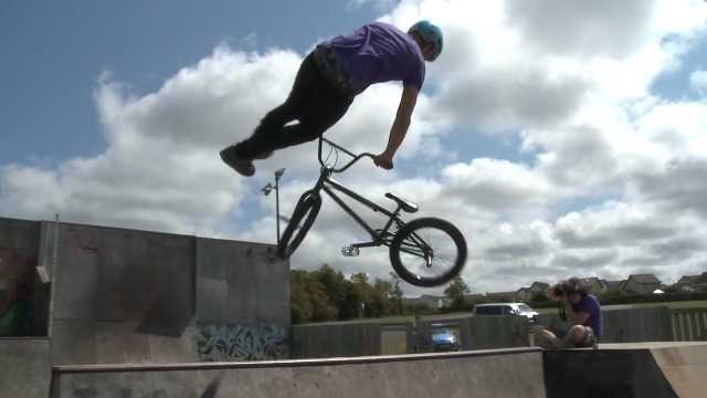
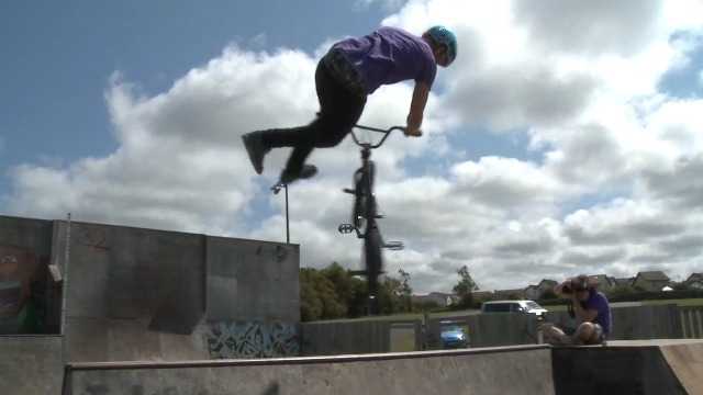
Figure 7 provides qualitative results of $\mathtt{LucidTracker}$ across three different datasets. Our system is robust to various challenges present in videos. It handles well camera view changes, fast motion, object shape deformation, out-of-view scenarios, multiple similar looking objects and even low quality video. We provide a detailed error analysis in section 5.5.

Conclusion

We show that top results can be obtained while using less training data. This shows that our lucid dreams leverage the available training data better. We report top results for this task while using only $24\negmedspace\sim\negmedspace 126$ training frames.

5.3 Ablation studies

In this section we explore in more details how the different ingredients contribute to our results.

5.3.1 Effect of training modalities

Table 2 compares the effect of different ingredients in the $\mathtt{Lucid}\mathtt{Tracker}^{-}$ training. Results are obtained using RGB and flow, with warping, no CRF, and no temporal coherency; $M_{t}\negmedspace=\negmedspace f\left(\mathcal{I}_{t},w(M_{t-1},\mathcal{F}_{t})\right)$.

Training from a single frame

In the bottom row ("only per-video tuning"), the model is trained per-video without ImageNet pre-training nor per-dataset training, i.e. using a single annotated training frame. Our network is based on VGG16 Chen2016ArxivDeeplabv2 and contains $\sim\negmedspace 20M$ parameters, all effectively learnt from a single annotated image that is augmented to become $2.5k$ training samples (see Section 4). Even with such minimal amount of training data, we still obtain a surprisingly good performance (compare $80.5$ on $\text{DAVIS}_{\text{16}}$ to others in Table 1). This shows how effective is, by itself, the proposed training strategy based on lucid dreaming of the data.

Variant	ImgNet pre-train.	per-dataset training	per-video fine-tun.	Dataset, mIoU
				$\text{DAVIS}_{\text{16}}$	YoutbObjs	$\mbox{SegTrck}_{\mbox{v2}}$
LucidTracker-	✓	✓	✓	83.7	76.2	76.8
(no ImgNet)	✗	✓	✓	82.0	74.3	71.2
No per-video tuning	✓	✓	✗	82.7	72.3	71.9
	✗	✓	✗	78.4	69.7	68.2
Only per- -video tuning	✓	✗	✓	79.4	-	70.4
	✗	✗	✓	80.5	-	66.8

Table 2: Ablation study of training modalities. ImageNet pre-training and per-video tuning provide additional improvement over per-dataset training. Even with one frame annotation for only per-video tuning we obtain good performance. See Section 5.3.1.

Pre-training & fine-tuning

We see that ImageNet pre-training does provide $2\negmedspace\sim\negmedspace 5$ percent point improvement (depending on the dataset of interest; e.g. $82.0\negmedspace\rightarrow\negmedspace 83.7\ \text{mIoU}$ on $\text{DAVIS}_{\text{16}}$). Per-video fine-tuning (after doing per-dataset training) provides an additional $1\negmedspace\sim\negmedspace 2$ percent point gain (e.g. $82.7\negmedspace\rightarrow\negmedspace 83.7\ \text{mIoU}$ on $\text{DAVIS}_{\text{16}}$). Both ingredients clearly contribute to the segmentation results.

Note that training a model using only per-video tuning takes about one full GPU day per video sequence; making these results insightful but not decidedly practical.

Preliminary experiments evaluating on $\text{DAVIS}_{\text{16}}$ the impact of the different ingredients of our lucid dreaming data generation showed, depending on the exact setup, $3\negmedspace\sim\negmedspace 10$ percent mIoU points fluctuations between a basic version (e.g. without non-rigid deformations nor scene re-composition) and the full synthesis process described in Section 4. Having a sophisticated data generation process directly impacts the segmentation quality.

Conclusion

Surprisingly, we discovered that per-video training from a single annotated frame provides already much of the information needed for the video object segmentation task. Additionally using ImageNet pre-training, and per-dataset training, provide complementary gains.

5.3.2 Effect of optical flow

Table 3 shows the effect of optical flow on $\mathtt{LucidTracker}$ results. Comparing our full system to the "No OF" row, we see that the effect of optical flow varies across datasets, from minor improvement in YouTubeObjects, to major difference in $\text{SegTrack}_{\text{v2}}$. In this last dataset, using mask warping is particularly useful too. We additionally explored tuning the optical flow stream per-video, which resulted in a minor improvement ($83.7\negmedspace\rightarrow\negmedspace 83.9\ \text{mIoU}$ on $\text{DAVIS}_{\text{16}}$).

Our "No OF" results can be compared to OSVOS Caelles2017Cvpr which does not use optical flow. However OSVOS uses a per-frame mask post-processing based on a boundary detector (trained on further external data), which provides $\sim\negmedspace 2$ percent point gain. Accounting for this, our "No OF" (and no CRF, no temporal coherency) result matches theirs on $\text{DAVIS}_{\text{16}}$ and YouTubeObjects despite using significantly less training data (see Table 1, e.g. $79.8-2\approx 78.0$ on $\text{DAVIS}_{\text{16}}$).

Table 4 shows the effect of using different optical flow estimation methods. For $\mathtt{LucidTracker}$ results, FlowNet2.0 IlgCVPR17 was employed. We also explored using EpicFlow EpicFlowCVPR15 , as in Khoreva2017CvprMaskTrack . Table 4 indicates that employing a robust optical flow estimation across datasets is crucial to the performance (FlowNet2.0 provides $\sim 1.5-15$ points gain on each dataset). We found EpicFlow to be brittle when going across different datasets, providing improvement for $\text{DAVIS}_{\text{16}}$ and $\text{SegTrack}_{\text{v2}}$ ($\sim 2-5$ points gain), but underperforming for YouTubeObjects ($74.7\negmedspace\rightarrow\negmedspace 71.3\ \text{mIoU}$).

Variant	$\mathcal{I}$	$\mathcal{F}$	warp.	Dataset, mIoU
			$w$	$\text{DAVIS}_{\text{16}}$	YoutbObjs	$\mbox{SegTrck}_{\mbox{v2}}$
LucidTracker	✓	✓	✓	86.6	77.3	78.0
LucidTracker-	✓	✓	✓	83.7	76.2	76.8
No warping	✓	✓	✗	82.0	74.6	70.5
No OF	✓	✗	✗	78.0	74.7	61.8
OF only	✗	✓	✓	74.5	43.1	55.8

Table 3: Ablation study of flow ingredients. Flow complements image only results, with large fluctuations across datasets. See Section 5.3.2.

Variant	Optical	Dataset, mIoU
	flow	$\text{DAVIS}_{\text{16}}$	YoutbObjs	$\mbox{SegTrck}_{\mbox{v2}}$
LucidTracker-	FlowNet2.0	83.7	76.2	76.8
	EpicFlow	80.2	71.3	67.0
	No flow	78.0	74.7	61.8
No ImageNet pre-training	FlowNet2.0	82.0	74.3	71.2
	EpicFlow	80.0	72.3	68.8
	No flow	76.7	71.4	63.0

Table 4: Effect of optical flow estimation.

Conclusion

The results show that flow provides a complementary signal to RGB image only and having a robust optical flow estimation across datasets is crucial. Despite its simplicity our fusion strategy ($f_{\mathcal{I}}+f_{\mathcal{F}}$ ) provides gains on all datasets, and leads to competitive results.

5.3.3 Effect of CRF tuning

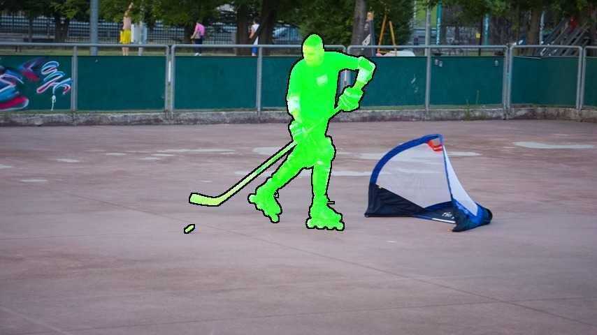	no CRF
	with CRF
	no CRF
	with CRF
1st frame, GT segment		$20\%$	$40\%$	$60\%$	$80\%$	$100\%$

Figure 8: Effect of CRF tuning. The shown $\text{DAVIS}_{\text{16}}$ videos have the highest margin between with and without CRF post-processing (based on mIoU over the video).

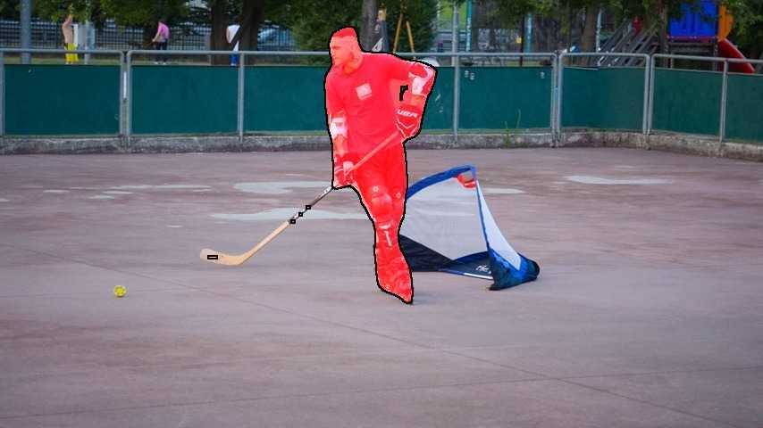
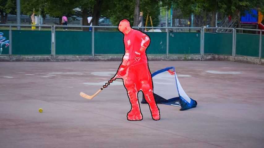
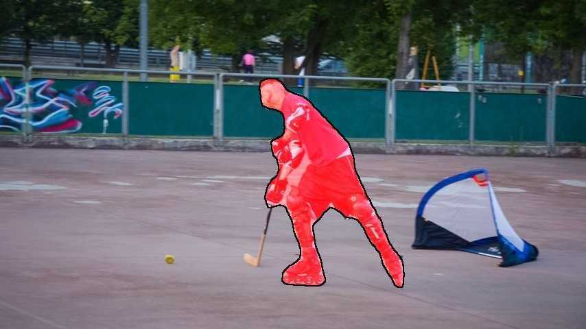
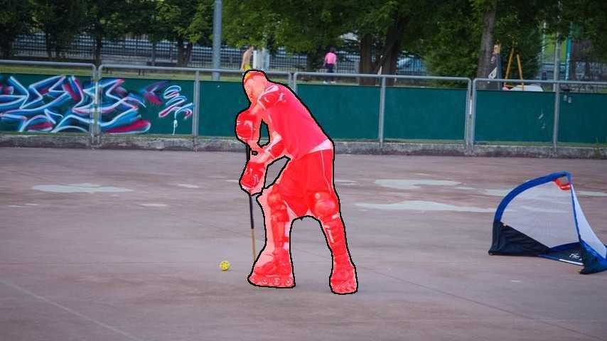
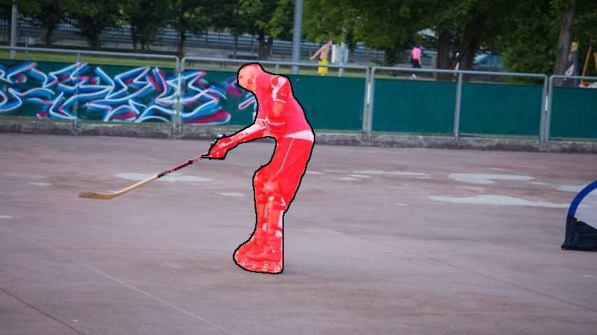
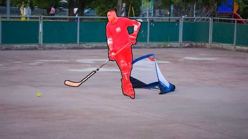
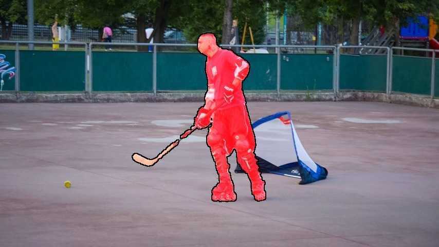
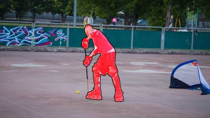
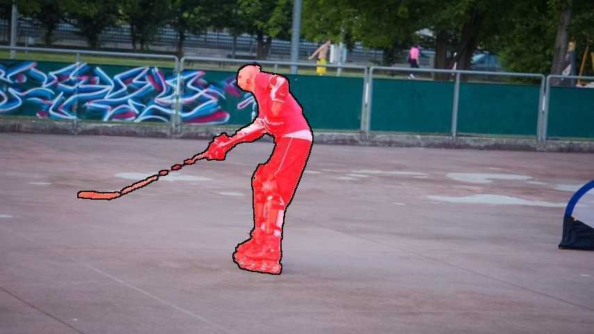
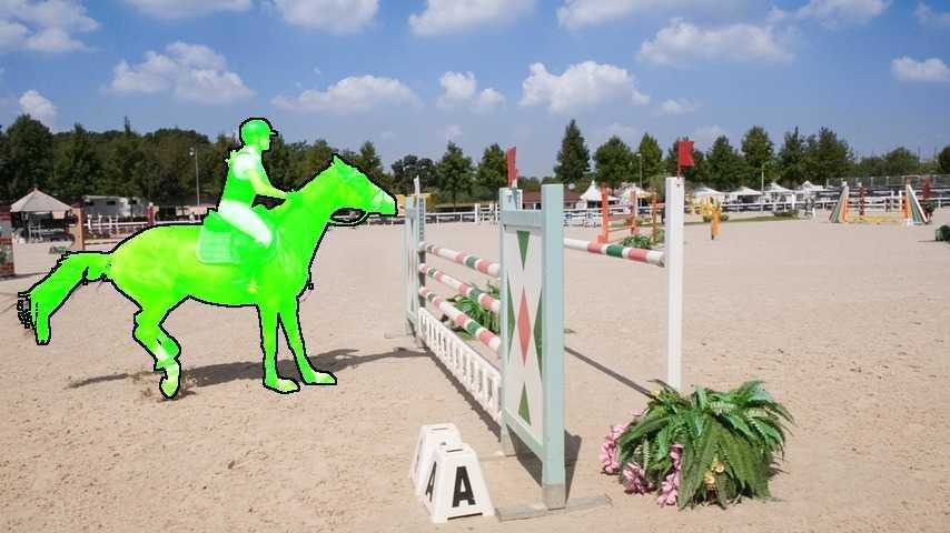
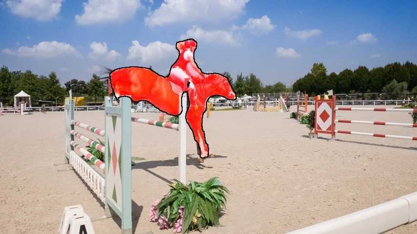
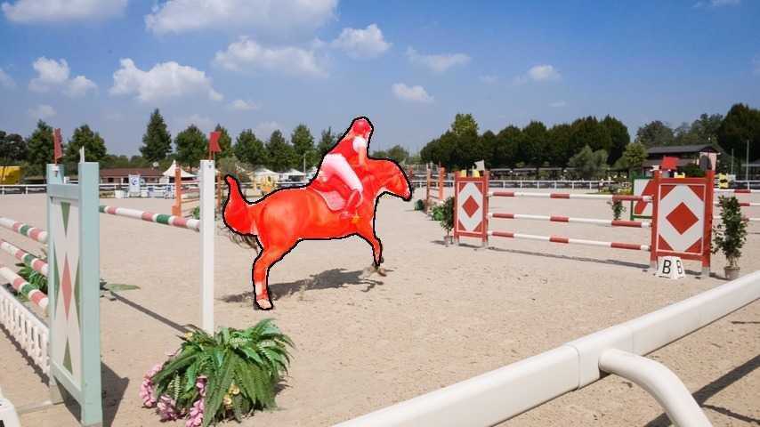
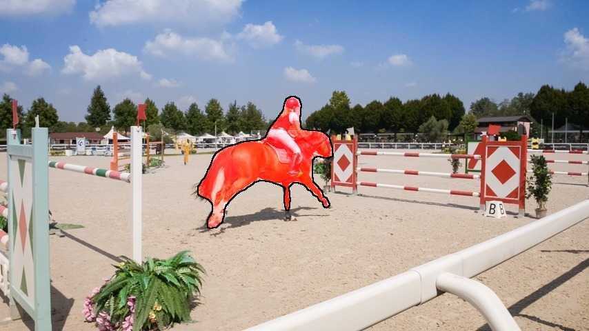
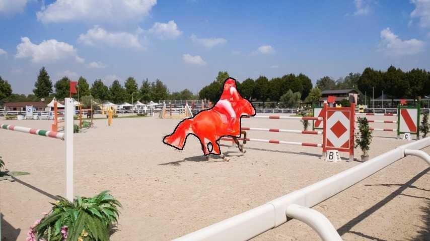
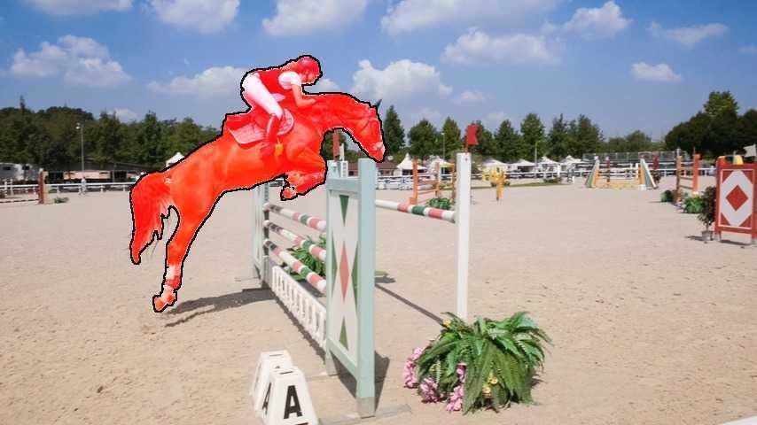
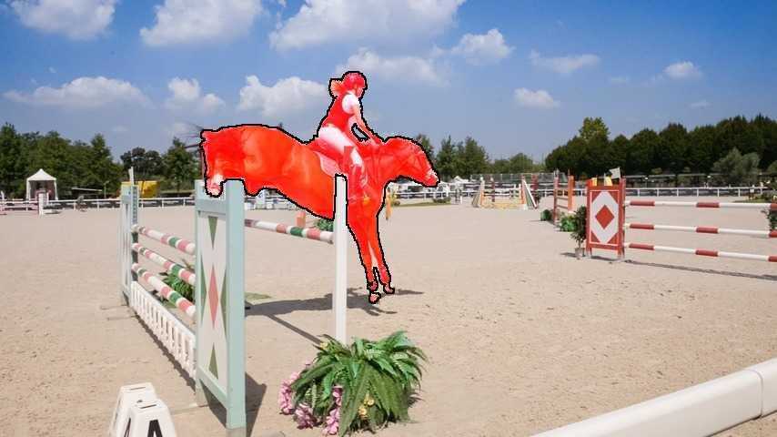
As a final stage of our pipeline, we refine the generated mask using DenseCRF Kraehenbuehl2011Nips per frame. This captures small image details that the network might have missed. It is known by practitioners that DenseCRF is quite sensitive to its parameters and can easily worsen results. We use our lucid dreams to enable automatic per-dataset CRF-tuning.

Following Chen2016ArxivDeeplabv2 we employ grid search scheme for tuning CRF parameters. Once the per-dataset model is trained, we apply it over a subset of its training set (5 random images from the lucid dreams per video sequence), apply DenseCRF with the given parameters over this output, and then compare to the lucid dream ground truth.

The impact of the tuned parameter of DenseCRF post-processing is shown in Table 5 and Figure 8. Table 5 indicates that without per-dataset tuning DenseCRF is under-performing. Our automated tuning procedure allows to obtain consistent gains without the need for case-by-case manual tuning.

Method	CRF	Dataset, mIoU
	parameters	$\text{DAVIS}_{\text{16}}$	YoutbObjs	$\mbox{SegTrck}_{\mbox{v2}}$
$\text{LucidTracker}^{-}$	-	83.7	76.2	76.8
$\text{LucidTracker}^{\ \ }$	default	84.2	75.5	72.2
$\text{LucidTracker}^{\ \ }$	tuned per-dataset	84.8	76.2	77.6

Table 5: Effect of CRF tuning ($\mathtt{LucidTracker}$ without temporal coherency). Without the automated per-dataset tuning DenseCRF will under-perform.

Conclusion

Using default DenseCRF parameters would degrade performance. Our lucid dreams enable automatic per-dataset CRF-tuning which allows to further improve the results.

5.4 Additional experiments

Other than adding or removing ingredients, as in Section 5.3, we also want to understand how the training data itself affects the obtained results.

5.4.1 Generalization across videos

Table 6 explores the effect of segmentation quality as a function of the number of training samples. To see more directly the training data effects we use a base model with RGB image $\mathcal{I}_{t}$ only (no flow $\mathcal{F}$, no CRF, no temporal coherency), and per-dataset training (no ImageNet pre-training, no per-video fine-tuning). We evaluate on two disjoint subsets of $15$ $\text{DAVIS}_{\text{16}}$ videos each, where the first frames for per-dataset training are taken from only one subset. The reported numbers are thus comparable within Table 6, but not across to the other tables in the paper. Table 6 reports results with varying number of training videos and with/without including the first frames of each test video for per-dataset training. When excluding the test set first frames, the image frames used for training are separate from the test videos; and we are thus operating across (related) domains. When including the test set first frames, we operate in the usual LucidTracker mode, where the first frame from each test video is used to build the per-dataset training set.

Comparing the top and bottom parts of the table, we see that when the annotated images from the test set video sequences are not included, segmentation quality drops drastically (e.g. $68.7\negmedspace\rightarrow\negmedspace 36.4\ \text{mIoU}$). Conversely, on subset of videos for which the first frame annotation is used for training, the quality is much higher and improves as the training samples become more and more specific (in-domain) to the target video ($65.4\negmedspace\rightarrow\negmedspace 78.3\ \text{mIoU}$). Adding extra videos for training does not improve the performance. It is better ($68.7\negmedspace\rightarrow\negmedspace 78.3\ \text{mIoU}$) to have $15$ models each trained and evaluated on a single video (row top-1-1) than having one model trained over $15$ test videos (row top-15-1).

Training with an additional frame from each video (we added the last frame of each train video) significantly boosts the resulting within-video quality (e.g. row top-30-2 $65.4\negmedspace\rightarrow\negmedspace 74.3\ \text{mIoU}$), because the training samples cover better the test domain.

	# training	# frames	mIoU
Training set	videos	per video
Includes 1st frames from test set	1	1	78.3
	2	1	75.4
	15	1	68.7
	30	1	65.4
	30	2	74.3
Excludes 1st frames from test set	2	1	11.6
	15	1	36.4
	30	1	41.7
	30	2	48.4

Table 6: Varying the number of training videos. A smaller training set closer to the target domain is better than a larger one. See Section 5.4.1.

Conclusion

These results show that, when using RGB information ($\mathcal{I}_{t}$), increasing the number of training videos does not improve the resulting quality of our system. Even within a dataset, properly using the training sample(s) from within each video matters more than collecting more videos to build a larger training set.

5.4.2 Generalization across datasets

Section 5.4.1 has explored the effect of changing the volume of training data within one dataset, Table 7 compares results when using different datasets for training. Results are obtained using a base model with RGB and flow ($M_{t}=f\left(\mathcal{I}_{t},\,M_{t-1}\right)$, no warping, no CRF, no temporal coherency), ImageNet pre-training, per-dataset training, and no per-video tuning to accentuate the effect of the training dataset.

The best performance is obtained when training on the first frames of the target set. There is a noticeable $\sim\negmedspace 10$ percent points drop when moving to the second best choice (e.g. $80.9\negmedspace\rightarrow\negmedspace 67.0$ for $\text{DAVIS}_{\text{16}}$). Interestingly, when putting all the datasets together for training ("all-in-one" row, a dataset-agnostic model) the results degrade, reinforcing the idea that "just adding more data" does not automatically make the performance better.

Conclusion

Best results are obtained when using training data that focuses on the test video sequences, using similar datasets or combining multiple datasets degrades the performance for our system.

Training set	Dataset, mIoU			Mean
	$\text{DAVIS}_{\text{16}}$	YoutbObjs	$\mbox{SegTrck}_{\mbox{v2}}$
$\text{DAVIS}_{\text{16}}$	80.9	50.9	46.9	59.6
YoutbObjs	67.0	71.5	52.0	63.5
$\mbox{SegTrack}_{\mbox{v2}}$	56.0	52.2	66.4	58.2
Best	80.9	71.5	66.4	72.9
Second best	67.0	52.2	52.0	57.1
All-in-one	71.9	70.7	60.8	67.8

Table 7: Generalization across datasets. Results with underline are the best per dataset, and in italic are the second best per dataset (ignoring all-in-one setup). We observe a significant quality gap between training from the target videos, versus training from other datasets; see Section 5.4.2.

5.4.3 Experimenting with the convnet architecture

Section 3.1 and Figure 3 described two possible architectures to handle $\mathcal{I}_{t}$ and $\mathcal{F}_{t}$. Previous experiments are all based on the two streams architecture.

Table 8 compares two streams versus one stream, where the network to accepts 5 input channels (RGB + previous mask + flow magnitude) in one stream: $M_{t}=f_{\mathcal{I+F}}\left(\mathcal{I}_{t}\right.$, $\mathcal{F}_{t}$, $\left.w(M_{t-1},\mathcal{\,F}_{t})\right)$. Results are obtained using a base model with RGB and optical flow (no warping, no CRF, no temporal coherency), ImageNet pre-training, per-dataset training, and no per-video tuning.

We observe that both one stream and two stream architecture with naive averaging perform on par. Using a one stream network makes the training more affordable and allows more easily to expand the architecture with additional input channels.

Architecture	ImgNet pre-train.	per-dataset training	per-video fine-tun.	$\text{DAVIS}_{\text{16}}$
				mIoU
two streams	✓	✓	✗	80.9
one stream	✓	✓	✗	80.3

Table 8: Experimenting with the convnet architecture. See Section 5.4.3.

Conclusion

The lighter one stream network performs as well as a network with two streams. We will thus use the one stream architecture in Section 6.

	Method	# training images	Flow $\mathcal{F}$	$\text{DAVIS}_{\text{16}}$
				Region, $J$			Boundary, $F$			Temporal stability, $T$
				Mean $\uparrow$	Recall $\uparrow$	Decay $\downarrow$	Mean $\uparrow$	Recall $\uparrow$	Decay $\downarrow$	Mean $\downarrow$
	Box oracle Khoreva2017CvprMaskTrack	0	✗	45.1	39.7	-0.7	21.4	6.7	1.8	1.0
	Grabcut oracle Khoreva2017CvprMaskTrack	0	✗	67.3	76.9	1.5	65.8	77.2	2.9	34.0
Ignores 1st frame annotation	Saliency	0	✗	32.7	22.6	-0.2	26.9	10.3	0.9	32.8
	NLC Faktor2014Bmvc	0	✓	64.1	73.1	8.6	59.3	65.8	8.6	35.8
	MP-Net Tokmakov2016Arxiv	~22.5k	✓	69.7	82.9	5.6	66.3	78.3	6.7	68.6
	Flow saliency	0	✓	70.7	83.2	6.7	69.7	82.9	7.9	48.2
	FusionSeg Jain2017ArxivFusionSeg	~95k	✓	71.5	-	-	-	-	-	-
	LVO TokmakovAS17	~35k	✓	75.9	89.1	0.0	72.1	83.4	1.3	26.5
	PDB Song_2018_ECCV	~18k	✗	77.2	90.1	0.9	74.5	84.4	-0.2	29.1
Uses 1st frame annotation	Mask warping	0	✓	32.1	25.5	31.7	36.3	23.0	32.8	8.4
	FCP Perazzi2015Iccv	0	✓	63.1	77.8	3.1	54.6	60.4	3.9	28.5
	BVS Maerki2016Cvpr	0	✗	66.5	76.4	26.0	65.6	77.4	23.6	31.6
	ObjFlow Tsai2016Cvpr	0	✓	71.1	80.0	22.7	67.9	78.0	24.0	22.1
	STV Wang2017ArxivSTV	0	✓	73.6	-	-	72.0	-	-	-
	VPN Jampani2016Arxiv	~2.3k	✗	75.0	-	-	72.4	-	-	29.5
	OSVOS Caelles2017Cvpr	~2.3k	✗	79.8	93.6	14.9	80.6	92.6	15.0	37.6
	MaskTrack Khoreva2017CvprMaskTrack	~11k	✓	80.3	93.5	8.9	75.8	88.2	9.5	18.3
	PReMVOS Luiten18ACCV	~145k	✓	84.9	96.1	8.8	88.6	94.7	9.8	19.7
	OnAVOS Voigtlaender2017OnlineAO	~120k	✗	86.1	96.1	5.2	84.9	89.7	5.8	19.0
	VideoGCRF Chandra2018DeepSR	~120k	✗	86.5	-	-	-	-	-	-
	LucidTracker	50	✓	86.6	97.3	5.3	84.8	93.1	7.5	15.9

Table 9: Comparison of video object segmentation results on $\text{DAVIS}_{\text{16}}$ benchmark. Numbers in italic are computed based on subsets of $\text{DAVIS}_{\text{16}}$. Our LucidTracker improves over previous results.

5.5 Error analysis

Table 9 presents an expanded evaluation on $\text{DAVIS}_{\text{16}}$ using evaluation metrics proposed in Perazzi2016Cvpr . Three measures are used: region similarity in terms of intersection over union (J), contour accuracy (F, higher is better), and temporal instability of the masks (T, lower is better). We outperform the competitive methods of Khoreva2017CvprMaskTrack ; Caelles2017Cvpr on all three measures.

Table 10 reports the per-attribute based evaluation as defined in $\text{DAVIS}_{\text{16}}$. $\mathtt{Lucid}$$\mathtt{Tracker}$ is best on all 15 video attribute categories. This shows that our $\mathtt{Lucid}$$\mathtt{Tracker}$ can handle the various video challenges present in $\text{DAVIS}_{\text{16}}$.

We present the per-sequence and per-frame results of $\mathtt{Lucid}$$\mathtt{Tracker}$ over $\text{DAVIS}_{\text{16}}$ in Figure 10. On the whole we observe that the proposed approach is quite robust, most video sequences reach an average performance above $80$ mIoU.

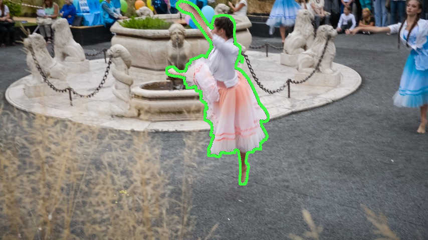
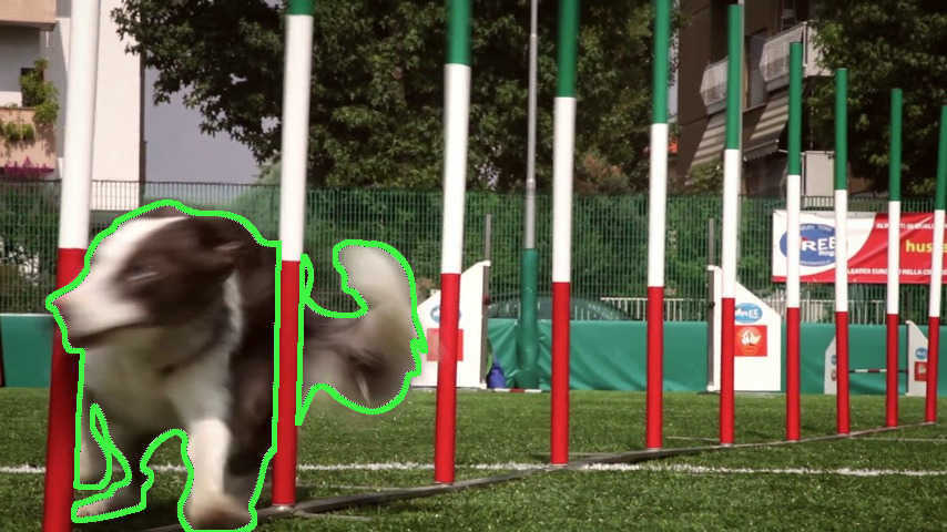
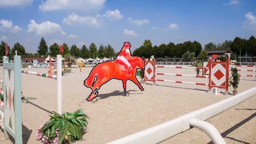
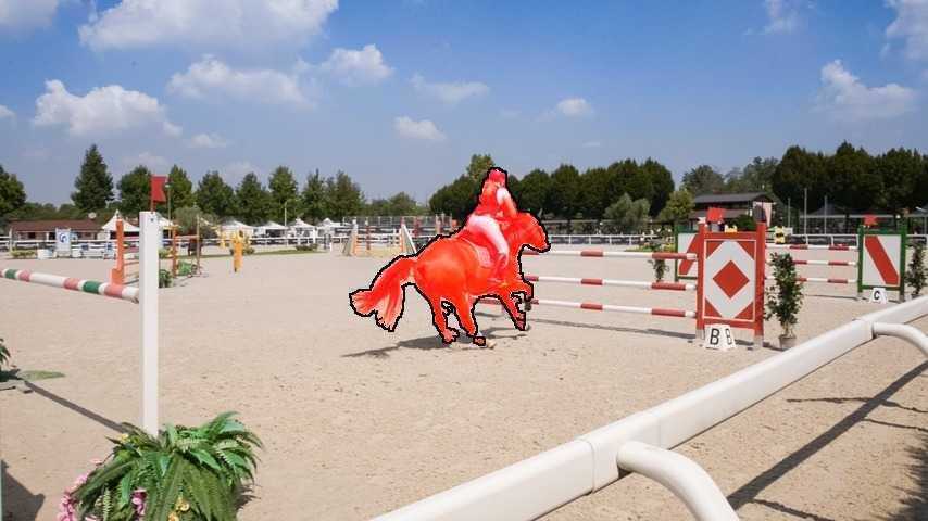
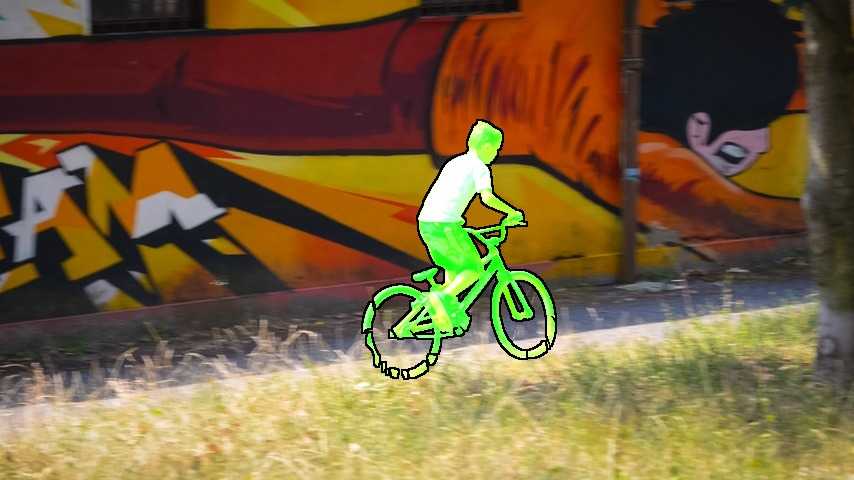
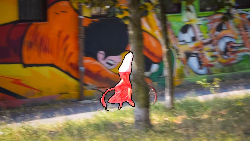
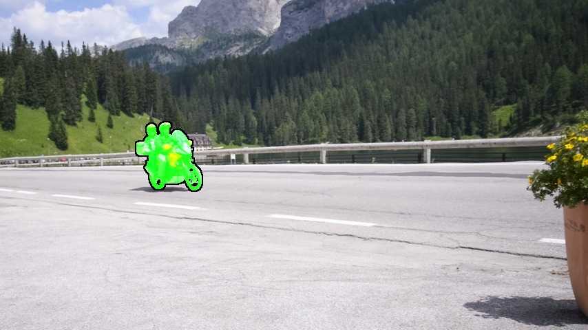
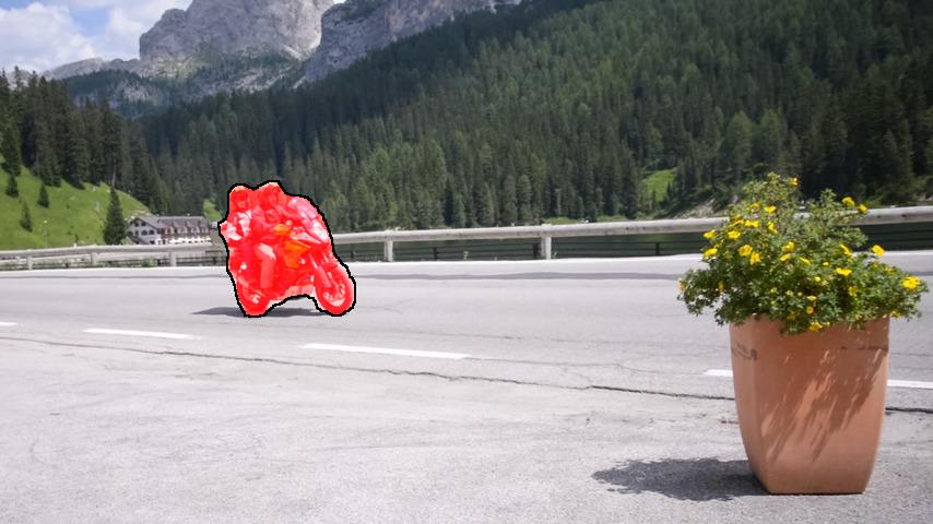
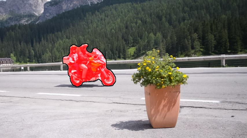
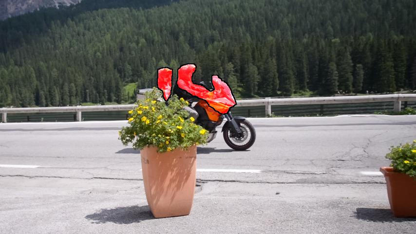
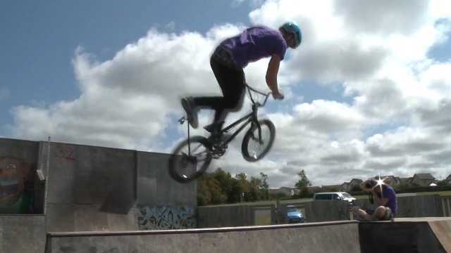
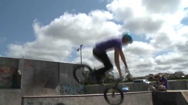
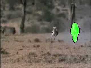
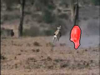
However, by looking at per-frame results for each video (blue dots in Figure 10) one can see several frames where our approach has failed (IoU less than $50$) to correctly track the object. Investigating closely those cases we notice conditions where $\mathtt{Lucid}$$\mathtt{Tracker}$ is more likely to fail. The same behaviour was observed across all three datasets. A few representatives of failure cases are visualized in Figure 9.

Since we are using only the mask annotation of the first frame for training the tracker, a clear failure case is caused by dramatic view point changes of the object from its first frame appearance, as in row 5 of Figure 9. Performing online adaptation every certain time step while exploiting the previous frame segments for data synthesis and marking unsure regions as ignore for training, similarly to Voigtlaender2017OnlineAO , might resolve the potential problems caused by relying only on the first frame mask. The proposed approach also under-performs when recovering from occlusions: it might takes several frames for the full object mask to re-appear (rows 1-3 in Figure 9). This is mainly due to the convnet having learnt to follow-up the previous frame mask. Augmenting the lucid dreams with plausible occlusions might help mitigate this case. Another failure case occurs when two similar looking objects cross each other, as in row 6 in Figure 9. Here both cues: the previous frame guidance and learnt via per-video tuning appearance, are no longer discriminative to correctly continue propagating the mask.

We also observe that the $\mathtt{Lucid}$$\mathtt{Tracker}$ struggles to track the fine structures or details of the object, e.g. wheels of the bicycle or motorcycle in rows 1-2 in Figure 9. This is the issue of the underlying choice of the convnet architecture, due to the several pooling layers the spatial resolution is lost and hence the fine details of the object are missing. This issue can be mitigated by switching to more recent semantic labelling architectures (e.g. pohlen2017FRRN ; ChenPSA17 ).

$\text{DAVIS}_{\text{16}}$
YouTubeObjects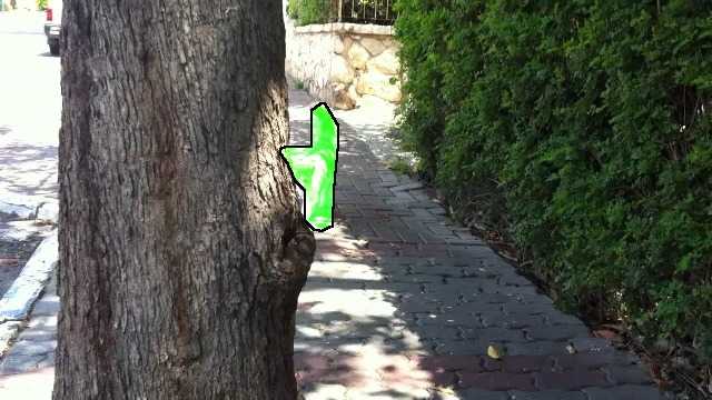
$\text{SegTrack}_{\text{v2}}$
	1st frame, GT segment	$20\%$	$40\%$	$60\%$	$80\%$	$100\%$

Figure 9: Failure cases. Frames sampled along the video duration (e.g. $50\%$: video middle point). For each dataset we show 2 out of 5 worst results (based on mIoU over the video).

Figure 10: Per-sequence results on $\text{DAVIS}_{\text{16}}$.

Attribute	Method
	BVS Maerki2016Cvpr	ObjFlow Tsai2016Cvpr	OSVOS Caelles2017Cvpr	MaskTrack Khoreva2017CvprMaskTrack	LucidTracker
Appearance change	0.46	0.54	0.81	0.76	0.84
Background clutter	0.63	0.68	0.83	0.79	0.86
Camera-shake	0.62	0.72	0.78	0.78	0.88
Deformation	0.7	0.77	0.79	0.78	0.87
Dynamic background	0.6	0.67	0.74	0.76	0.82
Edge ambiguity	0.58	0.65	0.77	0.74	0.82
Fast-motion	0.53	0.55	0.76	0.75	0.85
Heterogeneous object	0.63	0.66	0.75	0.79	0.85
Interacting objects	0.63	0.68	0.75	0.77	0.85
Low resolution	0.59	0.58	0.77	0.77	0.84
Motion blur	0.58	0.6	0.74	0.74	0.83
Occlusion	0.68	0.66	0.77	0.77	0.84
Out-of-view	0.43	0.53	0.72	0.71	0.84
Scale variation	0.49	0.56	0.74	0.73	0.81
Shape complexity	0.67	0.69	0.71	0.75	0.82

Table 10: $\text{DAVIS}_{\text{16}}$ per-attribute evaluation. LucidTracker improves across all video object segmentation challenges.

Conclusion

$\mathtt{LucidTracker}$ shows robust performance across different videos. However, a few failure cases were observed due to the underlying convnet architecture, its training, or limited visibility of the object in the first frame.

6 Multiple object segmentation results

We present here an empirical evaluation of LucidTracker for multiple object segmentation task: given a first frame labelled with the masks of several object instances, one aims to find the corresponding masks of objects in future frames.

1st frame, GT segment	$20\%$	$40\%$	$60\%$	$80\%$	$100\%$

Figure 11: LucidTracker qualitative results on $\text{DAVIS}_{\text{17}}$, test-dev set. Frames sampled along the video duration (e.g. $50\%$: video middle point). The videos are chosen with the highest mIoU measure.

6.1 Experimental setup

Dataset

For the multiple object segmentation task we use the 2017 DAVIS Challenge on Video Object Segmentation Pont-Tuset_arXiv_2017 ($\text{DAVIS}_{\text{17}}$). Compared to $\text{DAVIS}_{\text{16}}$ this is a larger, more challenging dataset, where the video sequences have multiple objects in the scene. Videos that have more than one visible object in $\text{DAVIS}_{\text{16}}$ have been re-annotated (the objects were divided by semantics) and the train and val sets were extended with more sequences. In addition, two other test sets (test-dev and test-challenge) were introduced. The complexity of the videos has increased with more distractors, occlusions, fast motion, smaller objects, and fine structures. Overall, $\text{DAVIS}_{\text{17}}$ consists of $150$ sequences, totalling $10\,474$ annotated frames and $384$ objects.

We evaluate our method on two test sets, the test-dev and test-challenge sets, each consists of $30$ video sequences, on average $\sim 3$ objects per sequence, the length of the sequences is $\sim 70$ frames. For both test sets only the masks on the first frames are made public, the evaluation is done via an evaluation server. Our experiments and ablation studies are done on the test-dev set.

Evaluation metric

The accuracy of multiple object segmentation is evaluated using the region (J) and boundary (F) measures proposed by the organisers of the challenge. The average of J and F measures is used as overall performance score (denoted as global mean in the tables). Please refer to Pont-Tuset_arXiv_2017 for more details about the evaluation protocol.

Training details

All experiments in this section are done using the single stream architecture discussed in sections 3.1 and 5.4.3. For training the models we use SGD with mini-batches of $10$ images and a fixed learning policy with initial learning rate of $10^{-3}$. The momentum and weight decay are set to $0.9$ and $5\cdot 10^{-4}$, respectively. All models are initialized with weights trained for image classification on ImageNet Simonyan2015Iclr . We then train per-video for 40k iterations.

6.2 Key results

Method	$\text{DAVIS}_{\text{17}}$, test-dev set
	Rank	Global mean $\uparrow$	Region, $J$			Boundary, $F$
			Mean $\uparrow$	Recall $\uparrow$	Decay $\downarrow$	Mean $\uparrow$	Recall $\uparrow$	Decay $\downarrow$
sidc	10	45.8	43.9	51.5	34.3	47.8	53.6	36.9
YXLKJ	9	49.6	46.1	49.1	22.7	53.0	56.5	22.3
haamooon DAVIS2017-4th	8	51.3	48.8	56.9	12.2	53.8	61.3	11.8
Fromandtozh DAVIS2017-7th	7	55.2	52.4	58.4	18.1	57.9	66.1	20.0
ilanv DAVIS2017-9th	6	55.8	51.9	55.7	17.6	59.8	65.8	18.9
voigtlaender DAVIS2017-5th	5	56.5	53.4	57.8	19.9	59.6	65.4	19.0
lalalafine123	4	57.4	54.5	61.3	24.4	60.2	68.8	24.6
wangzhe	3	57.7	55.6	63.2	31.7	59.8	66.7	37.1
lixx DAVIS2017-1st	2	66.1	64.4	73.5	24.5	67.8	75.6	27.1
LucidTracker	1	66.6	63.4	73.9	19.5	69.9	80.1	19.4

Table 11: Comparison of video object segmentation results on $\text{DAVIS}_{\text{17}}$, test-dev set. Our LucidTracker shows top performance.

Method	$\text{DAVIS}_{\text{17}}$, test-challenge set
	Rank	Global mean $\uparrow$	Region, $J$			Boundary, $F$
			Mean $\uparrow$	Recall $\uparrow$	Decay $\downarrow$	Mean $\uparrow$	Recall $\uparrow$	Decay $\downarrow$
zwrq0	10	53.6	50.5	54.9	28.0	56.7	63.5	30.4
Fromandtozh DAVIS2017-7th	9	53.9	50.7	54.9	32.5	57.1	63.2	33.7
wasidennis	8	54.8	51.6	56.3	26.8	57.9	64.8	28.8
YXLKJ	7	55.8	53.8	60.1	37.7	57.8	62.1	42.9
cjc DAVIS2017-6th	6	56.9	53.6	59.5	25.3	60.2	67.9	27.6
lalalafine123	6	56.9	54.8	60.7	34.4	59.1	66.7	36.1
voigtlaender DAVIS2017-5th	5	57.7	54.8	60.8	31.0	60.5	67.2	34.7
haamooon DAVIS2017-4th	4	61.5	59.8	71.0	21.9	63.2	74.6	23.7
vantam299 DAVIS2017-3rd	3	63.8	61.5	68.6	17.1	66.2	79.0	17.6
LucidTracker	2	67.8	65.1	72.5	27.7	70.6	79.8	30.2
lixx DAVIS2017-1st	1	69.9	67.9	74.6	22.5	71.9	79.1	24.1

Table 12: Comparison of video object segmentation results on $\text{DAVIS}_{\text{17}}$, test-challenge set. Our LucidTracker shows competitive performance, holding the second place in the competition.

Tables 12 and 12 presents the results of the 2017 DAVIS Challenge on test-dev and test-challenge sets Davis2017Challenge .

Our main results for the multi-object segmentation challenge are obtained via an ensemble of four different models ($f_{\mathcal{I}}$, $f_{\mathcal{I{\scriptscriptstyle+}F}}$, $f_{\mathcal{I{\scriptscriptstyle+}S}}$, $f_{\mathcal{I{\scriptscriptstyle+}F{\scriptscriptstyle+}\mathcal{S}}}$), see Section 3.1.

The proposed system, $\mathtt{Lucid}$$\mathtt{Tracker}$, provides the best segmentation quality on the test-dev set and shows competitive performance on the test-challenge set, holding the second place in the competition. The full system is trained using the standard ImageNet pre-training initialization, Pascal VOC12 semantic annotations for the $\mathcal{\mathcal{S}}_{t}$ input ($\sim\negmedspace 10k$ annotated images), and one annotated frame per test video, $30$ frames total on each test set. As discussed in Section 6.3, even without $\mathcal{\mathcal{S}}_{t}$ $\mathtt{Lucid}$$\mathtt{Tracker}$ obtains competitive results (less than $1$ percent point difference, see Table 13 for details).

The top entry $\mathtt{lixx}$ DAVIS2017-1st uses a deeper convnet model (ImageNet pre-trained ResNet), a similar segmentation architecture, trains it over external segmentation data (using $\sim\negmedspace 120k$ pixel-level annotated images from MS-COCO and Pascal VOC for pre-training, and akin to Caelles2017Cvpr fine-tuning on the $\text{DAVIS}_{\text{17}}$ train and val sets, $\sim\negmedspace 10k$ annotated frames), and extends it with a box-level object detector (trained over MS-COCO and Pascal VOC, $\sim\negmedspace 500k$ bounding boxes) and a box-level object re-identification model trained over $\sim\negmedspace 60k$ box annotations (on both images and videos). We argue that our system reaches comparable results with a significantly lower amount of training data.

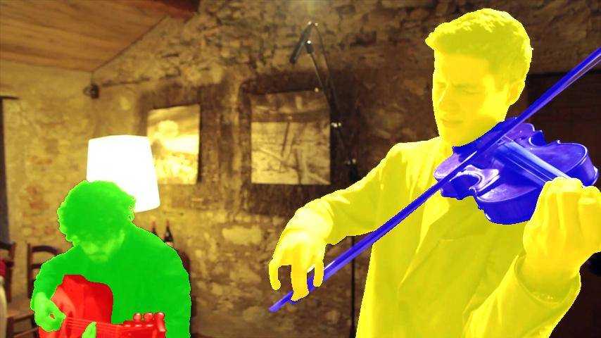
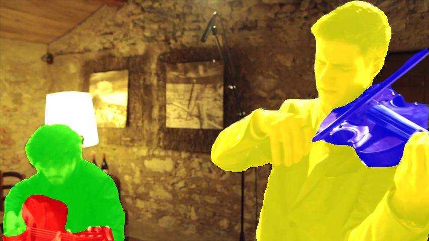
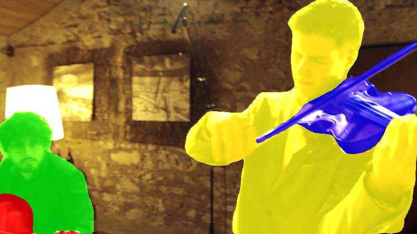
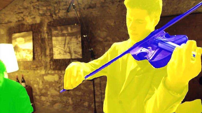
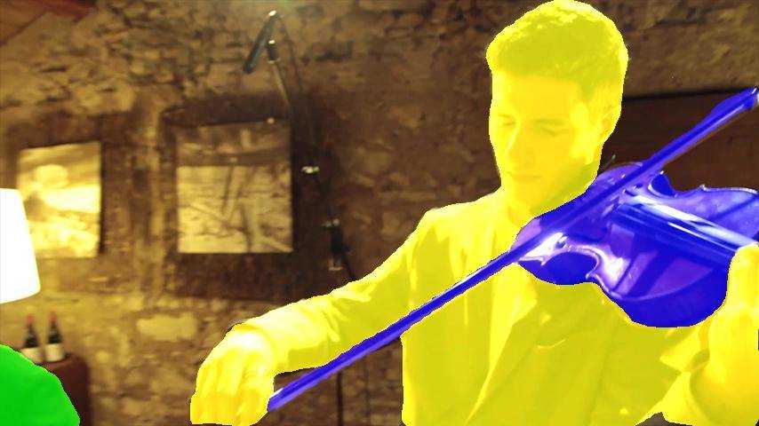
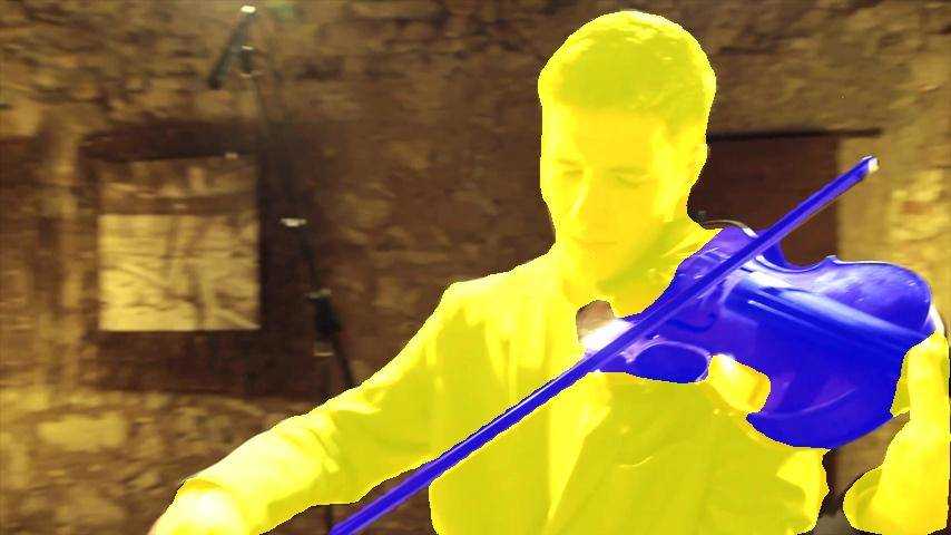
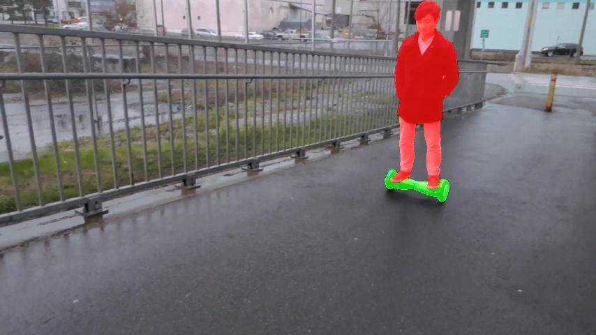
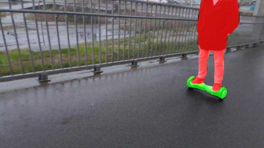
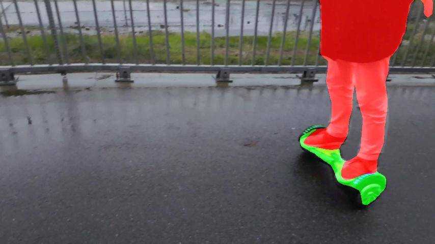
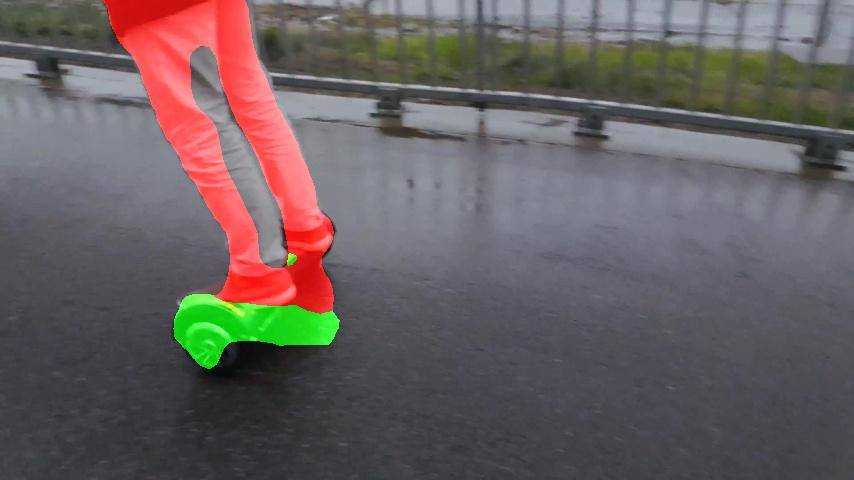
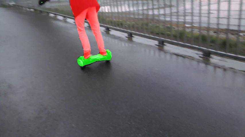
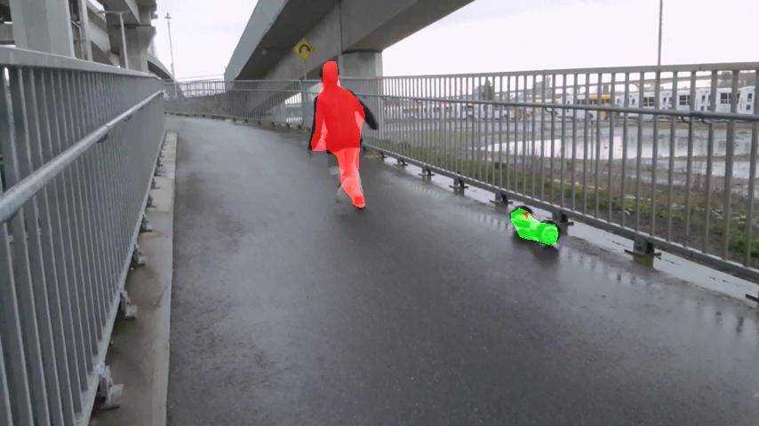
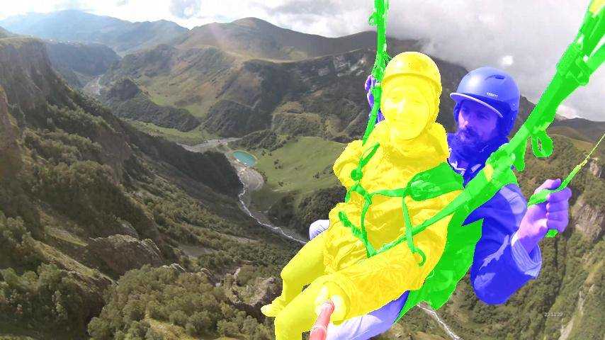
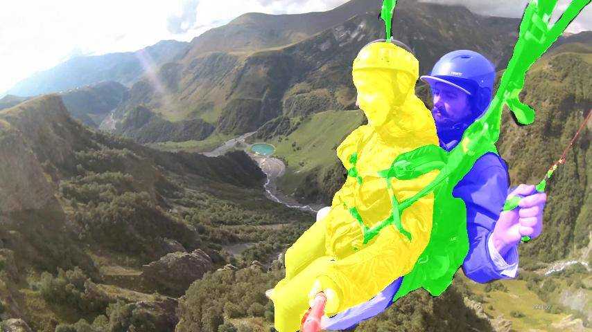
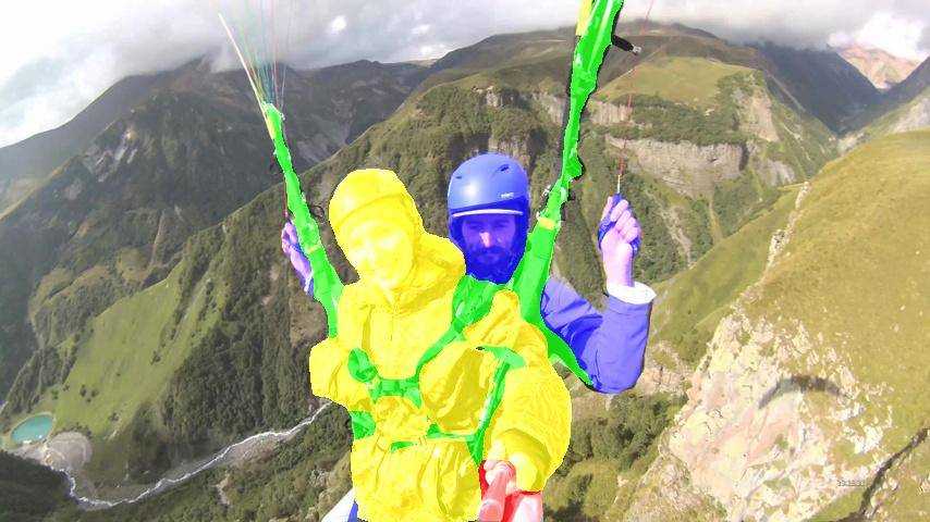
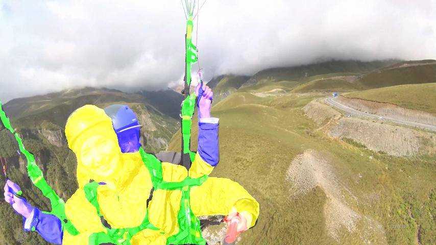
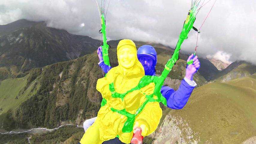
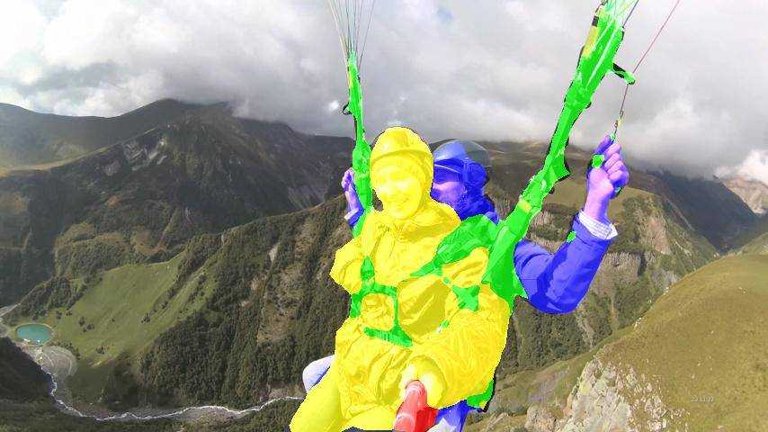
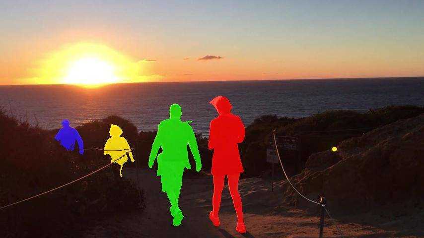
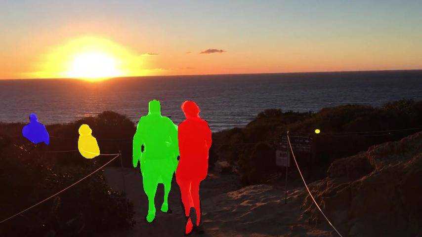
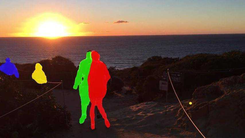
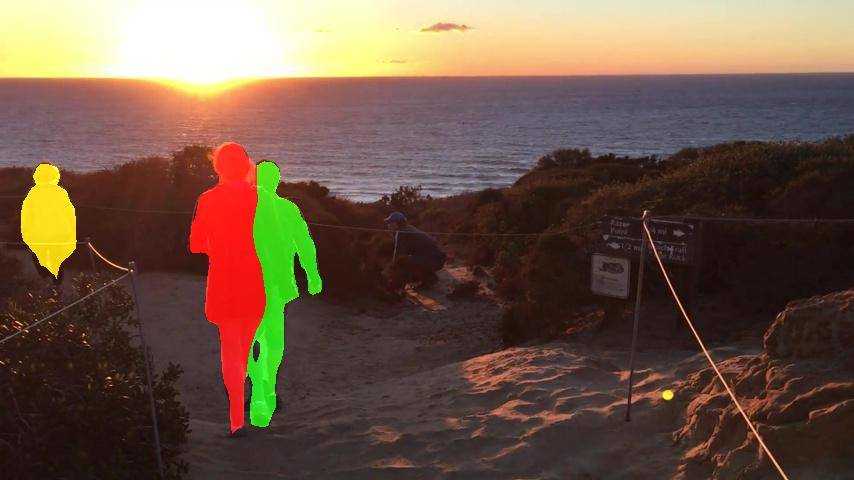
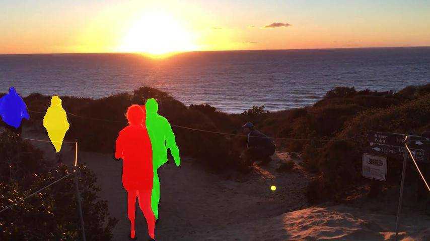
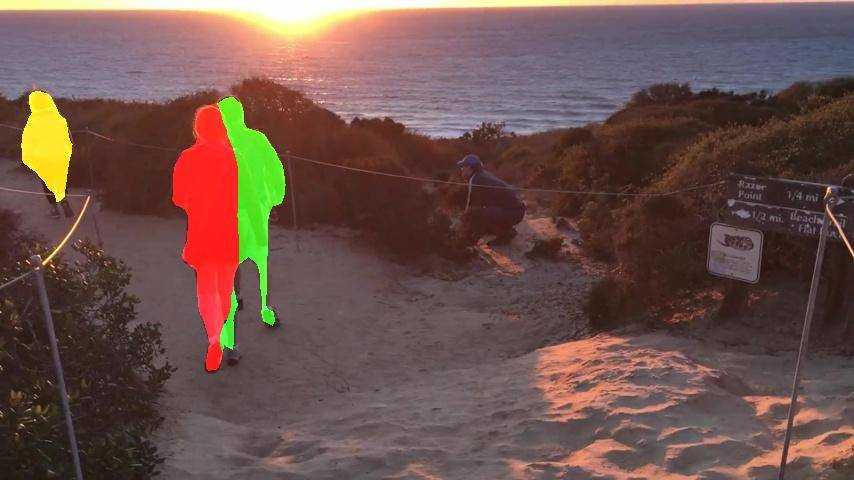
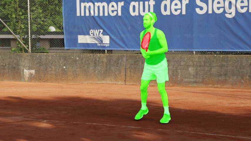
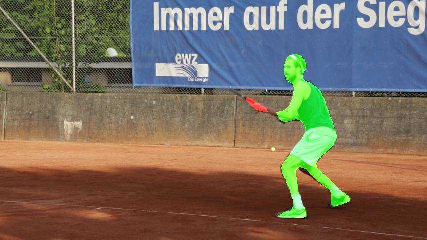
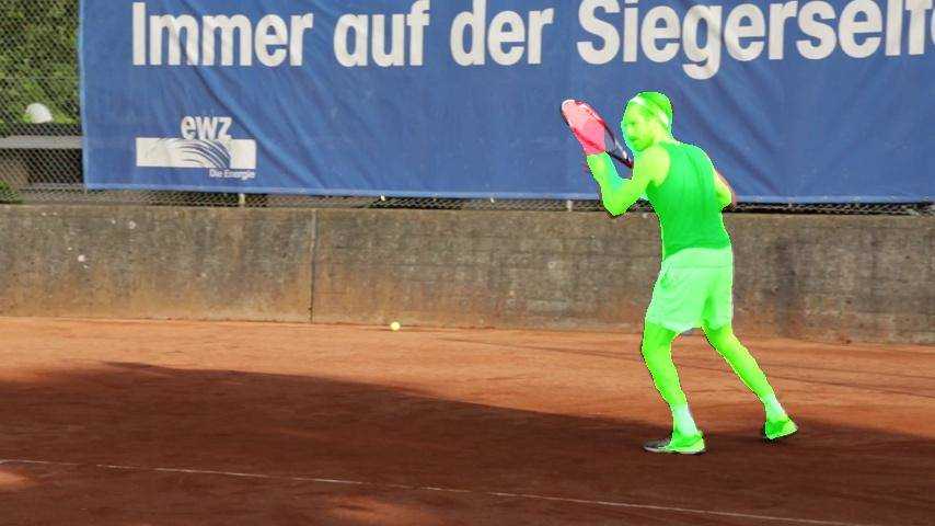
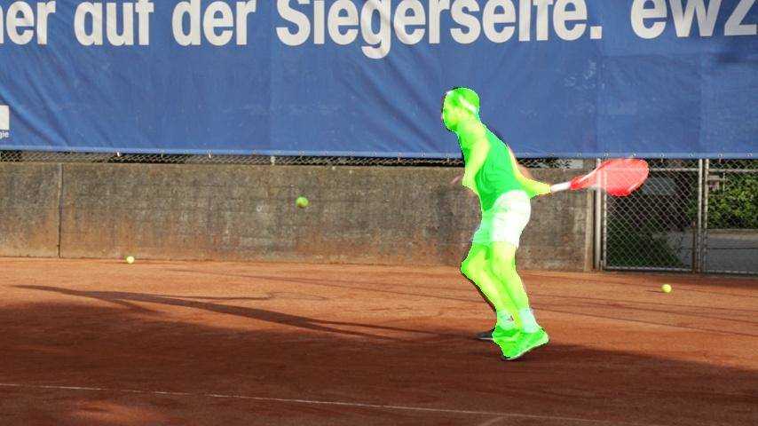
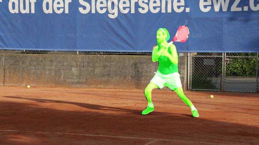
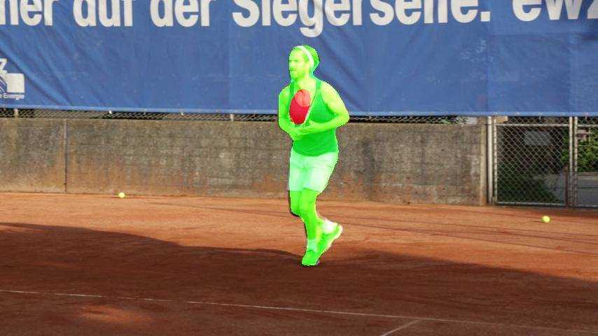
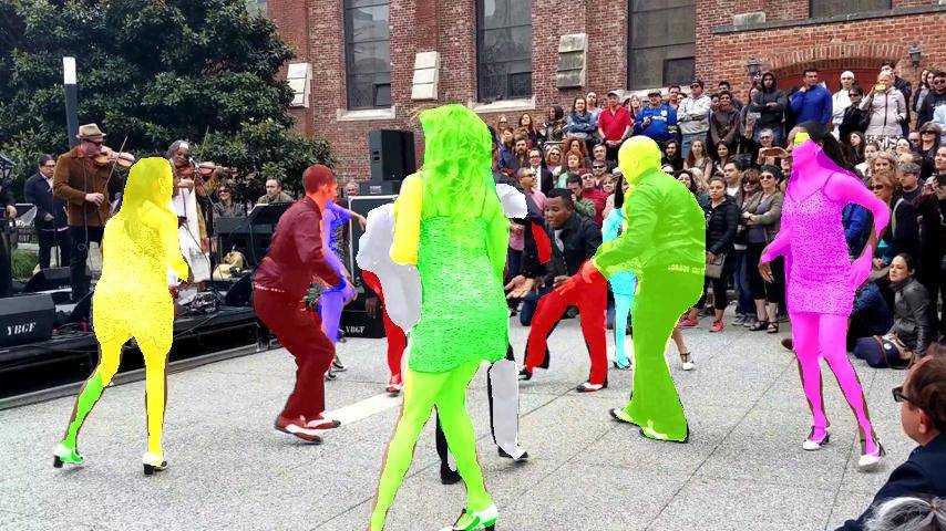
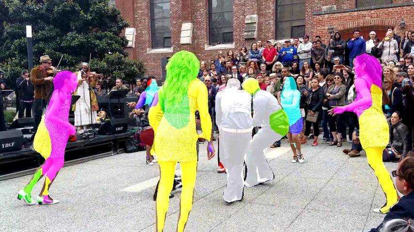
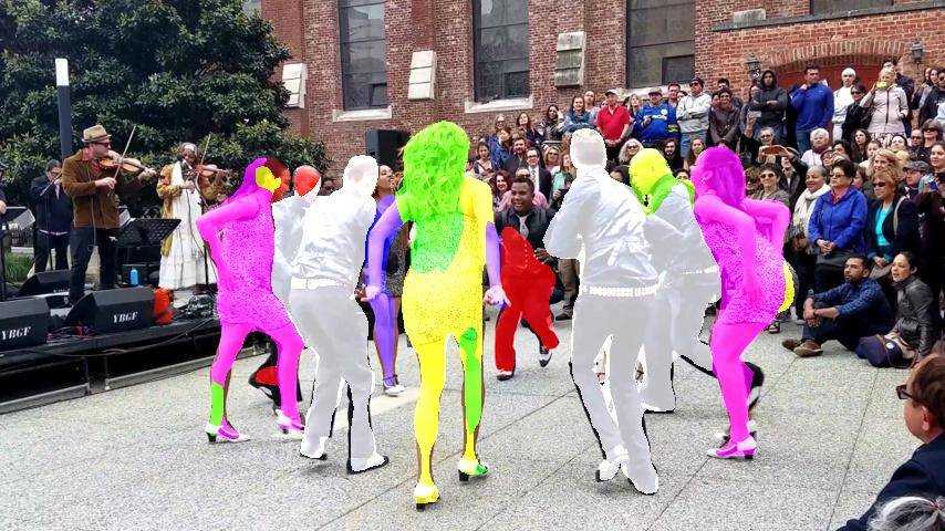
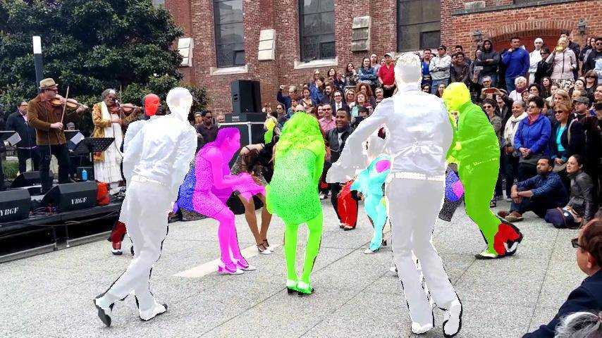
Figure 11 provides qualitative results of $\mathtt{Lucid}$$\mathtt{Tracker}$ on the test-dev set. The video results include successful handling of multiple objects, full and partial occlusions, distractors, small objects, and out-of-view scenarios.

Variant	$\mathcal{I}$	$\mathcal{F}$	$\mathcal{S}$	ensemble	CRF tuning	temp. coherency	$\text{DAVIS}_{\text{17}}$
							test-dev			test-challenge
							global mean	mIoU	mF	global mean	mIoU	mF
LucidTracker (ensemble)	✓	✓	✓	✓	✓	✓	66.6	63.4	69.9	67.8	65.1	70.6
	✓	✓	✓	✓	✓	✗	65.2	61.5	69.0	67.0	64.3	69.7
	✓	✓	✓	✓	✗	✗	64.7	60.5	68.9	66.5	63.2	69.8
	✓	✓	✗	✓	✓	✗	64.9	61.3	68.4	-	-	-
	✓	✓	✗	✓	✗	✗	64.2	60.1	68.3	-	-	-
LucidTracker	✓	✓	✓	✗	✓	✗	62.9	59.1	66.6	-	-	-
$\mathcal{I}+\mathcal{F}+\mathcal{S}$	✓	✓	✓	✗	✗	✗	62.0	57.7	62.2	64.0	60.7	67.3
$\mathcal{I}+\mathcal{F}$	✓	✓	✗	✗	✗	✗	61.3	56.8	65.8	-	-	-
$\mathcal{I}+\mathcal{S}$	✓	✗	✓	✗	✗	✗	61.1	56.9	65.3	-	-	-
$\mathcal{I}$	✓	✗	✗	✗	✗	✗	59.8	63.1	63.9	-	-	-

Table 13: Ablation study of different ingredients. $\text{DAVIS}_{\text{17}}$, test-dev and test challenge sets.

Conclusion

We show that top results for multiple object segmentation can be achieved via our approach that focuses on exploiting as much as possible the available annotation on the first video frame, rather than relying heavily on large external training data.

6.3 Ablation study

Table 13 explores in more details how the different ingredients contribute to our results.

We see that adding extra information (channels) to the system, either optical flow magnitude or semantic segmentation, or both, does provide $1\negmedspace\sim\negmedspace 2$ percent point improvement. The results show that leveraging semantic priors and motion information provides a complementary signal to RGB image and both ingredients contribute to the segmentation results.

Combining in ensemble four different models ($f_{\mathcal{I{\scriptscriptstyle+}F{\scriptscriptstyle+}\mathcal{S}}}+f_{\mathcal{I{\scriptscriptstyle+}F}}+f_{\mathcal{I{\scriptscriptstyle+}S}}+f_{\mathcal{I}}$ ) allows to enhance the results even further, bringing $2.7$ percent point gain ($62.0$ vs. $64.7$ global mean). Excluding the models which use semantic information ($f_{\mathcal{I{\scriptscriptstyle+}F{\scriptscriptstyle+}\mathcal{S}}}$ and $f_{\mathcal{I{\scriptscriptstyle+}S}}$) from the ensemble results only in a minor drop in the performance ($64.2$ vs. $64.7$ global mean). This shows that the competitive results can be achieved even with the system trained only with one pixel-level mask annotation per video, without employing extra annotations from Pascal VOC12.

Our lucid dreams enable automatic CRF-tuning (see Section 5.3.3) which allows to further improve the results ($64.7\negmedspace\rightarrow\negmedspace 65.2$ global mean). Employing the proposed temporal coherency step (see Section 3.1) during inference brings an additional performance gain ($65.2\negmedspace\rightarrow\negmedspace 66.6$ global mean).

Conclusion

The results show that both flow and semantic priors provide a complementary signal to RGB image only. Despite its simplicity our ensemble strategy provides additional gain and leads to competitive results. Notice that even without the semantic segmentation signal $\mathcal{\mathcal{S}}_{t}$ our ensemble result is competitive.

Figure 12: Per-sequence results on $\text{DAVIS}_{\text{17}}$, test-dev set.

1st frame, GT segment	$20\%$	$40\%$	$60\%$	$80\%$	$100\%$

Figure 13: LucidTracker failure cases on $\text{DAVIS}_{\text{17}}$, test-dev set. Frames sampled along the video duration (e.g. $50\%$: video middle point). We show 2 results mIoU over the video below 50.

6.4 Error analysis

We present the per-sequence results of $\mathtt{Lucid}$$\mathtt{Tracker}$ on $\text{DAVIS}_{\text{17}}$ in Figure 12 (per frame results not available from evaluation server). We observe that this dataset is significantly more challenging than $\text{DAVIS}_{\text{16}}$ (compare to Figure 10), with only $\nicefrac{{1}}{{3}}$ of the test videos above $80$ mIoU. This shows that multiple object segmentation is a much more challenging task than segmenting a single object.

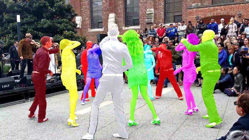
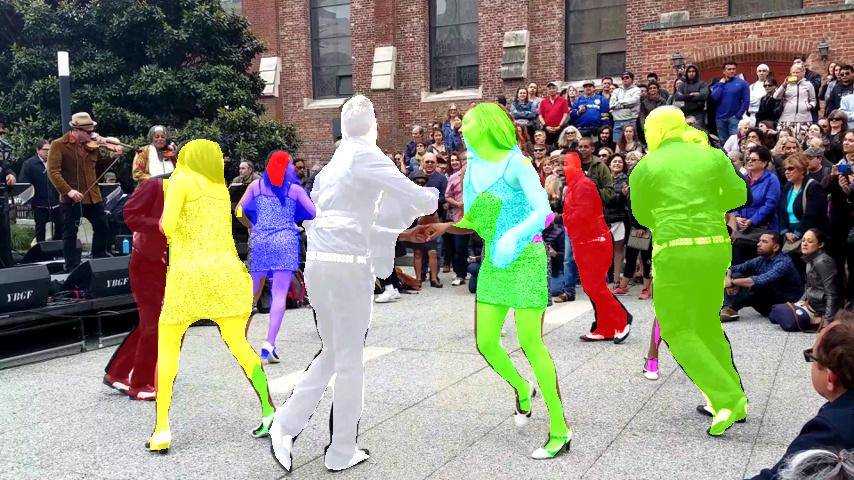
The failure cases discussed in Section 5.5 still apply to the multiple objects case. Additionally, on $\text{DAVIS}_{\text{17}}$ we observe a clear failure case when segmenting similar looking object instances, where the object appearance is not discriminative to correctly track the object, resulting in label switches or bleeding of the label to other look-alike objects. Figure 13 illustrates this case. This issue could be mitigated by using object level instance identification modules, like DAVIS2017-1st , or by changing the training loss of the model to more severely penalize identity switches.

Conclusion

In the multiple object case the $\mathtt{Lucid}$$\mathtt{Tracker}$ results remain robust across different videos. The overall results being lower than for the single object segmentation case, there is more room for future improvement in the multiple object pixel-level segmentation task.

7 Conclusion

We have described a new convnet-based approach for pixel-level object segmentation in videos. In contrast to previous work, we show that top results for single and multiple object segmentation can be achieved without requiring external training datasets (neither annotated images nor videos). Even more, our experiments indicate that it is not always beneficial to use additional training data, synthesizing training samples close to the test domain is more effective than adding more training samples from related domains.

Our extensive analysis decomposed the ingredients that contribute to our improved results, indicating that our new training strategy and the way we leverage additional cues such as semantic and motion priors are key.

Showing that training a convnet for video object segmentation can be done with only few ($\sim\negmedspace 100$) training samples changes the mindset regarding how much general knowledge about objects is required to approach this problem Khoreva2017CvprMaskTrack ; Jain2017ArxivFusionSeg , and more broadly how much training data is required to train large convnets depending on the task at hand.

We hope these new results will fuel the ongoing evolution of convnet techniques for single and multiple object segmentation in videos.

References

- (1) Ç. Aytekin, E. C. Ozan, S. Kiranyaz, and M. Gabbouj. Visual saliency by extended quantum cuts. In ICIP, 2015.
- (2) A. Bansal, X. Chen, B. Russell, A. Gupta, and D. Ramanan. Pixelnet: Representation of the pixels, by the pixels, and for the pixels. arXiv:1702.06506, 2017.
- (3) L. Bertinetto, J. Valmadre, J. F. Henriques, A. Vedaldi, and P. H. Torr. Fully-convolutional siamese networks for object tracking. arXiv:1606.09549, 2016.
- (4) F. Bookstein. Principal warps: Thin-plate splines and the decomposition of deformations. PAMI, 1989.
- (5) M. D. Breitenstein, F. Reichlin, B. Leibe, E. Koller-Meier, and L. Van Gool. Robust tracking-by-detection using a detector confidence particle filter. In ICCV, 2009.
- (6) S. Caelles, K.-K. Maninis, J. Pont-Tuset, L. Leal-Taixe, D. Cremers, and L. V. Gool. One-shot video object segmentation. In CVPR, 2017.
- (7) S. Chandra, C. Couprie, and I. Kokkinos. Deep spatio-temporal random fields for efficient video segmentation. In CVPR, 2018.
- (8) J. Chang, D. Wei, and J. W. Fisher. A video representation using temporal superpixels. In CVPR, 2013.
- (9) L. Chen, G. Papandreou, F. Schroff, and H. Adam. Rethinking atrous convolution for semantic image segmentation. arxiv: 1706.05587, 2017.
- (10) L.-C. Chen, G. Papandreou, I. Kokkinos, K. Murphy, and A. L. Yuille. Deeplab: Semantic image segmentation with deep convolutional nets, atrous convolution, and fully connected crfs. arXiv:1606.00915, 2016.
- (11) W. Chen, H. Wang, Y. Li, H. Su, Z. Wang, C. Tu, D. Lischinski, D. Cohen-Or, and B. Chen. Synthesizing training images for boosting human 3d pose estimation. In 3D Vision (3DV), 2016.
- (12) J. Cheng, S. Liu, Y.-H. Tsai, W.-C. Hung, S. Gupta, J. Gu, J. Kautz, S. Wang, and M.-H. Yang. Learning to segment instances in videos with spatial propagation network. CVPR Workshops, 2017.
- (13) A. Criminisi, P. Perez, and K. Toyama. Region filling and object removal by exemplar-based image inpainting. Trans. Img. Proc., 2004.
- (14) M. Danelljan, G. Hager, F. Shahbaz Khan, and M. Felsberg. Convolutional features for correlation filter based visual tracking. In ICCV Workshop, 2015.
- (15) A. Dosovitskiy, P. Fischer, E. Ilg, P. Häusser, C. Hazirbas, V. Golkov, P. v.d. Smagt, D. Cremers, and T. Brox. Flownet: Learning optical flow with convolutional networks. In ICCV, 2015.
- (16) M. Everingham, S. M. A. Eslami, L. Van Gool, C. K. I. Williams, J. Winn, and A. Zisserman. The pascal visual object classes challenge: A retrospective. IJCV, 2015.
- (17) A. Faktor and M. Irani. Video segmentation by non-local consensus voting. In BMVC, 2014.
- (18) G. Georgakis, A. Mousavian, A. C. Berg, and J. Kosecka. Synthesizing training data for object detection in indoor scenes. arXiv:1702.07836, 2017.
- (19) X. Glorot and Y. Bengio. Understanding the difficulty of training deep feedforward neural networks. In AISTATS, 2010.
- (20) M. Grundmann, V. Kwatra, M. Han, and I. Essa. Efficient hierarchical graph-based video segmentation. In CVPR, 2010.
- (21) A. Gupta, A. Vedaldi, and A. Zisserman. Synthetic data for text localisation in natural images. In CVPR, 2016.
- (22) D. Held, S. Thrun, and S. Savarese. Learning to track at 100 fps with deep regression networks. In ECCV, 2016.
- (23) J. F. Henriques, R. Caseiro, P. Martins, and J. Batista. Exploiting the circulant structure of tracking-by-detection with kernels. In ECCV, 2012.
- (24) E. Ilg, N. Mayer, T. Saikia, M. Keuper, A. Dosovitskiy, and T. Brox. Flownet 2.0: Evolution of optical flow estimation with deep networks. In CVPR, 2017.
- (25) B. L. J. Luiten, P. Voigtlaender. PReMVOS: Proposal-generation, refinement and merging for video object segmentation. In ACCV, 2018.
- (26) S. D. Jain and K. Grauman. Supervoxel-consistent foreground propagation in video. In ECCV, 2014.
- (27) S. D. Jain and K. Grauman. Click carving: Segmenting objects in video with point clicks. In HCOMP, 2016.
- (28) S. D. Jain, B. Xiong, and K. Grauman. Fusionseg: Learning to combine motion and appearance for fully automatic segmention of generic objects in videos. arXiv:1701.05384, 2017.
- (29) V. Jampani, R. Gadde, and P. V. Gehler. Video propagation networks. arXiv:1612.05478, 2016.
- (30) A. Khoreva, R. Benenson, E. Ilg, T. Brox, and B. Schiele. Lucid data dreaming for object tracking. CVPR Workshops, 2017.
- (31) A. Khoreva, F. Perazzi, R. Benenson, B. Schiele, and A. Sorkine-Hornung. Learning video object segmentation from static images. In arXiv:1612.02646, 2016.
- (32) P. Krähenbühl and V. Koltun. Efficient inference in fully connected crfs with gaussian edge potentials. In NIPS. 2011.
- (33) M. Kristan, J. Matas, et al. The visual object tracking vot2015 challenge results. In ICCV Workshop, 2015.
- (34) M. Kristan, J. Matas, et al. The visual object tracking vot2016 challenge results. In ECCV Workshop, 2016.
- (35) M. Kristan, R. Pflugfelder, et al. The visual object tracking vot2014 challenge results. In ECCV Workshop, 2014.
- (36) T. N. Le, K. T. Nguyen, M. H. Nguyen-Phan, T. V. Ton, T. A. Nguyen, X. S. Trinh, Q. H. Dinh, V. T. Nguyen, A. D. Duong, A. Sugimoto, T. V. Nguyen, and M. T. Tran. Instance re-identification flow for video object segmentation. CVPR Workshops, 2017.
- (37) F. Li, T. Kim, A. Humayun, D. Tsai, and J. M. Rehg. Video segmentation by tracking many figure-ground segments. In ICCV, 2013.
- (38) X. Li, Y. Qi, Z. Wang, K. Chen, Z. Liu, J. Shi, P. Luo, C. C. Loy, and X. Tang. Video object segmentation with re-identification. CVPR Workshops, 2017.
- (39) G. Lin, A. Milan, C. Shen, and I. D. Reid. Refinenet: Multi-path refinement networks for high-resolution semantic segmentation. arXiv:1611.06612, 2016.
- (40) C. Ma, J.-B. Huang, X. Yang, and M.-H. Yang. Hierarchical convolutional features for visual tracking. In ICCV, 2015.
- (41) N. Maerki, F. Perazzi, O. Wang, and A. Sorkine-Hornung. Bilateral space video segmentation. In CVPR, 2016.
- (42) N. Nagaraja, F. Schmidt, and T. Brox. Video segmentation with just a few strokes. In ICCV, 2015.
- (43) H. Nam, M. Baek, and B. Han. Modeling and propagating cnns in a tree structure for visual tracking. arXiv:1608.07242, 2016.
- (44) H. Nam and B. Han. Learning multi-domain convolutional neural networks for visual tracking. In CVPR, 2016.
- (45) N.Mayer, E.Ilg, P.Häusser, P.Fischer, D.Cremers, A.Dosovitskiy, and T.Brox. A large dataset to train convolutional networks for disparity, optical flow, and scene flow estimation. In CVPR, 2016.
- (46) A. Papazoglou and V. Ferrari. Fast object segmentation in unconstrained video. In ICCV, 2013.
- (47) D. Park and D. Ramanan. Articulated pose estimation with tiny synthetic videos. In CVPR Workshop, 2015.
- (48) D. Pathak, R. Girshick, P. Dollár, T. Darrell, and B. Hariharan. Learning features by watching objects move. arXiv:1612.06370, 2016.
- (49) F. Perazzi, J. Pont-Tuset, B. McWilliams, L. V. Gool, M. Gross, and A. Sorkine-Hornung. A benchmark dataset and evaluation methodology for video object segmentation. In CVPR, 2016.
- (50) F. Perazzi, O. Wang, M. Gross, and A. Sorkine-Hornung. Fully connected object proposals for video segmentation. In ICCV, 2015.
- (51) L. Pishchulin, A. Jain, M. Andriluka, T. Thormählen, and B. Schiele. Articulated people detection and pose estimation: Reshaping the future. In CVPR, 2012.
- (52) T. Pohlen, A. Hermans, M. Mathias, and B. Leibe. Full-resolution residual networks for semantic segmentation in street scenes. In CVPR, 2017.
- (53) J. Pont-Tuset, F. Perazzi, S. Caelles, P. Arbeláez, A. Sorkine-Hornung, and L. Van Gool. Davis challenge on video object segmentation 2017. http://davischallenge.org/challenge2017.
- (54) J. Pont-Tuset, F. Perazzi, S. Caelles, P. Arbeláez, A. Sorkine-Hornung, and L. Van Gool. The 2017 davis challenge on video object segmentation. arXiv:1704.00675, 2017.
- (55) A. Prest, C. Leistner, J. Civera, C. Schmid, and V. Ferrari. Learning object class detectors from weakly annotated video. In CVPR, 2012.
- (56) J. Revaud, P. Weinzaepfel, Z. Harchaoui, and C. Schmid. Epicflow: Edge-preserving interpolation of correspondences for optical flow. In CVPR, 2015.
- (57) S. R. Richter, V. Vineet, S. Roth, and V. Koltun. Playing for data: Ground truth from computer games. In ECCV, 2016.
- (58) C. Rother, V. Kolmogorov, and A. Blake. Grabcut: Interactive foreground extraction using iterated graph cuts. In SIGGRAPH, 2004.
- (59) A. Shaban, A. Firl, A. Humayun, J. Yuan, X. Wang, P. Lei, N. Dhanda, B. Boots, J. M. Rehg, and F. Li. Multiple-instance video segmentation with sequence-specific object proposals. CVPR Workshops, 2017.
- (60) G. Sharir, E. Smolyansky, and I. Friedman. Video object segmentation using tracked object proposals. CVPR Workshops, 2017.
- (61) K. Simonyan and A. Zisserman. Very deep convolutional networks for large-scale image recognition. In ICLR, 2015.
- (62) H. Song, W. Wang, S. Zhao, J. Shen, and K.-M. Lam. Pyramid dilated deeper convlstm for video salient object detection. In ECCV, 2018.
- (63) T. V. Spina and A. X. Falcão. Fomtrace: Interactive video segmentation by image graphs and fuzzy object models. arXiv:1606.03369, 2016.
- (64) J. Sun, J. Jia, C.-K. Tang, and H.-Y. Shum. Poisson matting. In SIGGRAPH, 2004.
- (65) K. Tang, V. Ramanathan, L. Fei-fei, and D. Koller. Shifting weights: Adapting object detectors from image to video. In NIPS, 2012.
- (66) M. Tang, D. Marin, I. Ben Ayed, and Y. Boykov. Normalized cut meets mrf. In ECCV, 2016.
- (67) S. Tang, M. Andriluka, A. Milan, K. Schindler, S. Roth, and B. Schiele. Learning people detectors for tracking in crowded scenes. In ICCV, 2013.
- (68) R. Tao, E. Gavves, and A. W. Smeulders. Siamese instance search for tracking. arXiv:1605.05863, 2016.
- (69) P. Tokmakov, K. Alahari, and C. Schmid. Learning motion patterns in videos. arXiv:1612.07217, 2016.
- (70) P. Tokmakov, K. Alahari, and C. Schmid. Learning video object segmentation with visual memory. In ICCV, 2017.
- (71) Y.-H. Tsai, M.-H. Yang, and M. J. Black. Video segmentation via object flow. In CVPR, 2016.
- (72) G. Varol, J. Romero, X. Martin, N. Mahmood, M. J. Black, I. Laptev, and C. Schmid. Learning from synthetic humans. arXiv:1701.01370.
- (73) P. Voigtlaender and B. Leibe. Online adaptation of convolutional neural networks for the 2017 davis challenge on video object segmentation. CVPR Workshops, 2017.
- (74) P. Voigtlaender and B. Leibe. Online adaptation of convolutional neural networks for video object segmentation. In BMVC, 2017.
- (75) T. Vojir and J. Matas. Pixel-wise object segmentations for the VOT 2016 dataset. Research report, 2017.
- (76) L. Wang, W. Ouyang, X. Wang, and H. Lu. Visual tracking with fully convolutional networks. In ICCV, 2015.
- (77) T. Wang, B. Han, and J. Collomosse. Touchcut: Fast image and video segmentation using single-touch interaction. CVIU, 2014.
- (78) W. Wang and J. Shen. Super-trajectory for video segmentation. arXiv:1702.08634, 2017.
- (79) X. Wang and A. Gupta. Unsupervised learning of visual representations using videos. In ICCV, 2015.
- (80) Z. Wu, C. Shen, and A. van den Hengel. Wider or deeper: Revisiting the resnet model for visual recognition. arXiv:1611.10080, 2016.
- (81) F. Xiao and Y. J. Lee. Track and segment: An iterative unsupervised approach for video object proposals. In CVPR, 2016.
- (82) J. J. Yu, A. W. Harley, and K. G. Derpanis. Back to basics: Unsupervised learning of optical flow via brightness constancy and motion smoothness. arXiv:1608.05842, 2016.
- (83) H. Zhao. Some promising ideas about multi-instance video segmentation. CVPR Workshops, 2017.
- (84) H. Zhao, J. Shi, X. Qi, X. Wang, and J. Jia. Pyramid scene parsing network. In CVPR, 2017.
- (85) Y. Zhu, Z. Lan, S. Newsam, and A. G. Hauptmann. Guided optical flow learning. arXiv:1702.02295, 2017.