Learned Spectral Super-Resolution

Abstract

We describe a novel method for blind, single-image spectral super-resolution. While conventional super-resolution aims to increase the spatial resolution of an input image, our goal is to spectrally enhance the input, i.e., generate an image with the same spatial resolution, but a greatly increased number of narrow (hyper-spectral) wavelength bands. Just like the spatial statistics of natural images has rich structure, which one can exploit as prior to predict high-frequency content from a low resolution image, the same is also true in the spectral domain: the materials and lighting conditions of the observed world induce structure in the spectrum of wavelengths observed at a given pixel. Surprisingly, very little work exists that attempts to use this diagnosis and achieve blind spectral super-resolution from single images. We start from the conjecture that, just like in the spatial domain, we can learn the statistics of natural image spectra, and with its help generate finely resolved hyper-spectral images from RGB input. Technically, we follow the current best practice and implement a convolutional neural network (CNN), which is trained to carry out the end-to-end mapping from an entire RGB image to the corresponding hyperspectral image of equal size. We demonstrate spectral super-resolution both for conventional RGB images and for multi-spectral satellite data, outperforming the state-of-the-art.

1 Introduction

Single-image super-resolution is a challenging computer vision problem with many interesting applications, e.g. in the fields of astronomy, medical imaging and law enforcement. The goal is to infer, from a single low-resolution image, the missing high frequency content that would be visible in a corresponding high resolution image. The problem itself is inherently ill-posed, extremely so for large upscaling factors. Still, several successful schemes have been designed [10]. The key is to exploit the high degree of structure in the visual world and design or learn a prior that constrains the solution accordingly.

Figure 1: Spectral super-resolution: our method is able to predict fine-grained hyperspectral images, using only a single RGB image as input (number of output channels reduced for visualisation, actual output has 31 bands of width 10 nm).

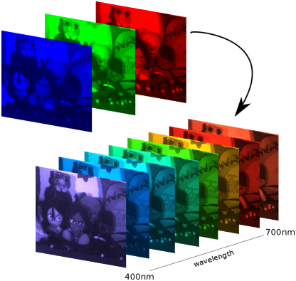
Indeed there is a large body of literature on single-image super-resolution, which is however largely limited to the spatial domain. Very few authors address the complementary problem, to increase the spectral resolution of the input image beyond the coarse RGB channels. The topic of this paper is single-image spectral super-resolution. We pose the obvious question whether we can also learn the spectral structure of the visual world, and use it as a prior to predict hyper-spectral images with finer spectral resolution from a standard RGB image. Note the trade-off between spatial and spectral information, even at the sensor level: to obtain a reasonable signal-to-noise ratio, cameras can have small pixels and integrate over large spectral bands; or they can have fine spectral resolution, but integrate over large pixels.

Depending on the available images and the application, it may be useful to increase the resolution in space or to obtain a finer quantisation of the visible spectrum. While in the spatial domain the restoration of missing high-frequency information reveals smaller objects and more accurate boundaries, high-frequency spectral information makes it easier to separate the spectral signatures of different objects and materials that have similar RGB color. The extra information included in the recovered hyper-spectral (HS) image bands enables applications like tracking [37], segmentation [35], face recognition [30], document analysis [22, 29], analysis of paintings [12], food inspection [39] and image classification [6].

A related, but simpler problem has been studied by several authors, namely hyper-spectral super-resolution [2, 18, 24, 33]. There, one assumes that both a HS image of low spatial resolution and an RGB image with finer resolution are available, and the two are fused to get the best of both worlds. The desired output is thus the same as in our problem — but requires an additional input. Our work can be seen as an attempt to do away with the spatially coarse hyper-spectral image and learn a generic prior for hyper-spectral signatures.

The problem is heavily under-constrained: for typical terrestrial applications, the goal is to generate, for each pixel, $\approx$30 spectral bands from the 3 input channels. The difference is even more extreme in aerial and satellite remote sensing, where the low-resolution image has at most 10 channels covering the visible and infrared range, whereas hyper-spectral images routinely have $>$200 bands over the same range. Still, there is evidence that blind spectral super-resolution is possible. For practical processing, hyper-spectral signatures are sometimes projected to a lower-dimensional subspace [4], indicating that there is a significant amount of correlation between their bands. Moreover, most scenes consist of a limited number of materials, distributed in characteristic patterns. Thus, there is hope that one can learn them from a suitable training set. Here, we do exactly that: we train a convolutional neural network (CNN) to predict the missing high-frequency detail of the colour spectrum observed at each pixel.

There are two main differences to spatial super-resolution, which has also been tackled with CNNs. First, spatial super-resolution has the convenient property that training data can be obtained by downsampling existing images of the desired resolution, so training data is available for free in virtually unlimited quantities. This is not the case for our problem, because hyper-spectral cameras are not a ubiquitous consumer product, and training data is comparatively rare. We nevertheless manage to obtain enough training data even if we are constrained to a more limited amount of image. In cases where the overall number of images is small we regularize the solution with an Euclidean penalized and additionally augment the training data by flipping and rotating input images. Second, and more importantly, the point spread functions of different cameras are rather similar and in general steep, whereas the spectral response (the “spectral blur kernel”) of the color channels can vary significantly from sensor to sensor. The latter means that an individual super-resolution has to be learned for each camera type.

2 Related Work

Single-image super-resolution usually corresponds to spatially upsampling a single low-resolution RGB image to higher spatial resolution. This has been a popular topic for several years, and quite some literature exists. Early method attempted to devise clever upsampling functions, sometimes by manually analyzing the image statistics, while recently the trend has been to learn dictionaries of image patches, often in combination with a sparsity prior [36, 43, 47]. Lately, CNNs have boosted the performance of super-resolution, showing significant improvements [9, 20, 21]. They are also able to perform the task in real time [32]. Interestingly, the RMSE does not seem to be the best loss function to obtain visually convincing upsampling results. Other loss functions aiming for “photo-realism” better match human perception, although the actual intensity differences are higher [26].

On the other hand hyperspectral super-resolution uses as input a low resolution hyperspectral and an RGB image to create a high resolution hyperspectral output. There are two main schools. Some methods require only known spectral response of the RGB camera, but can correct for spatial mis-alignment known [1, 2, 18]. Others assume that also the registration between the two input images is perfectly known [24, 33, 38, 41, 45].

Our work also has some relation to the problem of image colorization, where a grayscale image is spectrally upsampled to RGB, i.e., from one channel to three. There CNNs have also shown promising results [25, 48] by converting the input to a Lab colorspace and predicting the ab channels.

Acquiring a hyperspectral image by using only an RGB camera has been attempted with the help of active lighting [7]. This can be achieved by using spectral filters in front of the illumination, with the main disadvantage that the method can only be used in the laboratory. A similar idea is to use tunable narrow-band filters and take multiple images, such that narrow spectral bands are recorded sequentially [13]. Taking a step further from tuning the hardware, Wug et al. [40] proposed the use of multiple RGB images from different cameras, which are combined to obtain a single hyper-spectral image — effectively turning the differences between the camera’s spectral responses into an advantage. All these solutions require dedicated hardware as well as a static scene.

On the contrary, attempts to reconstruct hyper-spectral information from a single RGB image are rare. Nguyen et al. [28] use a radial basis function network to model the mapping from RGB values to scene reflectance. They assume the camera’s spectral response function is perfectly known (and, as a by-product, also estimate the spectral illumination). More recently, Arad et al. [3] proposed to learn sparse dictionary with K-SVD as hyper-spectral upsampling prior. Assuming the spectral response of the RGB camera is known, they then use Orthogonal Matching Pursuit (OMP) to reconstruct the hyper-spectral signal using from the RGB intensities. Closely related methods exist for spatial super-resolution [47] as well as hyper-spectral super-resolution [1]. The two methods are closely related the only main technical difference is on which images are used to learn the dictionary. Zeyde et al. [47] employ low resolution hyperspectral image as prior while Akhtar et al. [1] compute their prior on a similar image contained inside their dataset.

To summarize, several constrained versions of the spectral super-resolution problem have been investigated. But we believe that our work is the first generic framework that requires only a single RGB image, no knowledge of the spectral response functions, can be used indoors and outdoors, and needs neither a static scene nor special filter hardware.

Figure 2: Diagram of our network for spectral super resolution. Skip connection propagate the information copying and concatenating the output from earlier layers. The multi scale structure allows to explore the whole spatial extent of the input image. Note that, except for the first convolutions, the other blocks are made of a dense block as in [17]

Figure 3: Depiction of a single Densenet block

3 Method

In our work we follow the current rend in computer vision research and learn the desired super-resolution mapping end-to-end with a (convolutonal) neural network. In the following we present the network architecture and give implementation details.

Figure 4: Comparison of reconstructed radiance to the ground truth values. Two images from ICVL dataset with the same range as presented by Arad and Ben-Shahar et al. [3]

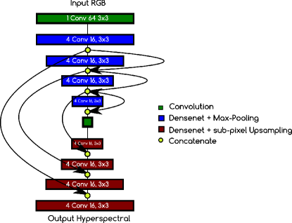
Selecting a network architecture for deep learning is not straightforward for a novel application, where no prior studies point to suitable designs. It is however clear that, for our purposes, the output should have the same image size as the input (but more channels). We thus build on recent work in semantic segmentation. Our proposed network is a variant of the semantic segmentation architecture Tiramisu of Jégou et al. [17], which in turn is based on the Densenet [16] architecture for classification. As a first measure, we replace the loss function and use an Euclidean loss, since we face a regression-type problem: instead of class labels (respectively, class scores) our network shall predict the continuously varying intensities for all spectral bands. Additionally, since we are interested in the high fidelity representation of each pixel we replace the original deconvolution layer with subpixel upsampling as proposed by the super-resolution work of Shi et al. [32].

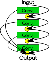
The Tiramisu network has further interesting properties for our task. Skip connections, within and across Densenet blocks (see 2, 3) perform concatenation instead of summation of layers, as opposed to ResNet [14]. They greatly speed up the learning and alleviate the vanishing gradient problem. More importantly, its architecture is based on a multiscale paradigm which allows the network to learn the overall image structure, while keeping the image resolution constant. In the Tiramisu structure, each downscaling step is done with a convolutional layer of size $1$ and $\max$-pooling, while for each resolution level a single Densenet is used, with varying number of convolutional layers.

Our network architecture, with a total of 56 layers, is depicted in Fig. 2 where, if otherwise specified, each convolution has size $3\times 3$.

The image gets down-scaled 5 times by a factor of 2, with a $1\times 1$ convolution followed by $\max$-pooling. In it’s own terminology, each Densenet block has a growth rate of 4 with 16 layers, which means 4 convolutional layers per block, each with 16 filters, see Fig. 3. For a more details about the Densenet/Tiramisu architecture, please refer to the original papers [16, 17].

For each image in the training dataset we randomly sample a set of patches of size $64\times 64$ and directly feed them to the neural network. At test time, where the goal is to reconstruct the complete image, we tile the input into $64\times 64$ tiles, with 8 pixels overlap to avoid boundary artifacts.

3.1 Relation to spectral unmixing

Often, hyper-spectral images are interpreted in terms of “endmembers” and “abundances”: the endmembers can be imagined as the pure spectra of the observed materials and form a natural basis. Observed pixel spectra are additive combinations of endmembers, with the abundances (proportions of different materials) as coefficients.

Dong et al. [9] showed how a shallow CNN for super-resolution can be interpreted in terms of basis learning and reconstruction. In much the same manner, our CNN can be seen as an implicit, non-linear extension of the unmixing model, where the knowledge about the endmembers at both low and high spectral resolution is embedded in the convolution weights. The forward pass through the network can be thought of as first extracting the abundances from the input and then multiplying them with the learned endmembers to obtain the hyperspectral output image.

3.2 Implementation details

The network, implemented with Keras [8], is trained from scratch, using the Adam optimizer [23] with Nesterov moment [34, 11]. We iterate it for $100$ epochs with learning rate $0.002$, then for another $200$ epoch with learning rate $0.0002$, the rest of the parameters follows those provided in the paper. We initialize our model with HeUniform [15], and apply $50\%$ dropout in the convolutional layers to avoid overfitting. Moreover, we found it crucial to carefully tune the Euclidean regularization, probably due to the general lack of copious amount of images on the training set. We fix it to $10^{-6}$, higher values lead to overly smooth, less accurate solutions.

Figure 5: Qualitative comparison w.r.t. [28] over three non consecutive spectral bands.

4 Results

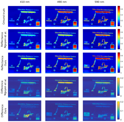
We evaluate our result on four different datasets. Where possible, we compare it with the other two methods [3, 28] that are also able to estimate an hyperspectral image from an single RGB. Note, both baselines need the spectral response of the RGB camera to be known. Hence, we feed it to them as additional input, contrary to our method. Despite the disadvantage, our CNN super-resolution is more accurate, see below.

Error computation

We evaluate w.r.t. three different error metric over 8bit images (as far as they are available): root mean square error (RMSE), relative root mean square error (RMSERel), and the spectral angle mapper (SAM) [46], i.e., the average angular deviation between the estimated pixel spectra, measured in degrees. We would like to highlight how we measure RMSERel and RMSE as there is not a common agreement on its computation. RMSE is obtained by computing it on 8bit and clipping values higher and lower than the allowed range. For RMSERel we normalized the predicted image by the mean of the ground truth.

4.1 Training data

We follow the standard practice for quantitative evaluation and synthetically generate the input data, given the difficulties of capturing separate hyper-spectral and RGB images that are aligned and have comparable resolution and sharpness. I.e., the RGB image is emulated by integrating over hyper-spectral channels according to a predefined camera response function. We always use the response functions provided by the authors, to ensure the images are strictly the same and the comparisons are fair. If a dataset already provides a train/test split, we follow it. Otherwise, we run two-fold cross-validation: split the dataset in two, train on the first half to predict the second half and vice versa.

Table 1: Comparison of our method with Arad et al. [3] on ICVL and CAVE dataset.

	ICVL		CAVE
	Ours	Arad et al. [3]	Ours	Arad et al. [3]
RMSE	1.980	2.633	4.76	5.4
RMSERel	0.0587	0.0756	0.2804	–
SAM	2.04	–	12.10	–

4.2 ICVL dataset

The ICVL dataset has been released by Arad and Ben-Shahar [3], together with their method. It contains 201 images acquired using a line scanner camera (Specim PS Kappa DX4 hyperspectral), mounted on a rotary stage for spatial scanning. The dataset contains a variety of scenes captured both indoors and outdoors, including man-made to natural objects. Images were originally captured with a spatial resolution of 1392$\times$1300 over 519 spectral bands (400-1,000nm ) but have been downsampled to 31 spectral channels from 400nm to 700nm at 10nm increments. We map the hyperspectral images to RGB using CIE 1964 color matching functions, like in the original paper.

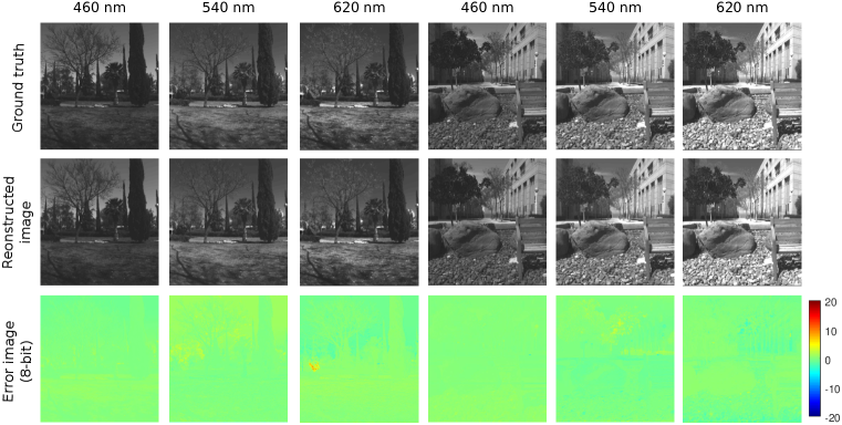
There, a sparse dictionary is learned with K-SVD as hyper-spectral upsampling prior. However, they do not use a global train/test split, as we do. Rather, they divide the dataset into subsets of images that show the same type of scene (such as parks or indoor environments), hold out one test image per subset, and train on the remaining ones; thus learning a different prior for each test image that is specifically tuned to the scene type. We prefer to keep the prior generic and use a single, global train/test split. We then predict their held-out images, but using the same network for all that fall into the first, respectively second half of our split. Even so, our results are competitive, see Table 1. We are not able to reproduce their method due to missing parameter or availability of code, instead we show the same figures presented in their paper in Fig. 4.

Figure 6: Prediction from spectral image, ground truth and difference images for a subregion of a Hyperion satellite image. The bands shown are 0,20,40 (first row), 60,80,120 (second row), corresponding to the following central frequencies in nm: 426, 630, 833, 1013, 1215, 1618. Note the reconstruction quality across different bands, and that the difference images are in fact dominated by typical sensor noise patterns like streaking artifacts.

Table 2: Error evaluated on 8-bit images over the radiance w.r.t. [28] on NUS dataset

	RMSE	RMSERel	SAM
Nguyen et al. [28]	8.99	0.324	9.23
Ours	5.27	0.234	10.11

Table 3: Error evaluation on the reflectance using the same procedure as in [28] on NUS dataset

	RMSE	RMSERel	SAM
Nguyen et al. [28]	0.0451	0.3070	10.37
Ours	0.0390	0.2406	11.94

Figure 7: Ground truth, prediction and difference of one image of NUS dataset. Note how the marked line artifacts in the ground truth gets removed by our method.

4.3 NUS dataset

The NUS dataset [28] contains the spectral irradiance and spectral illumination (400-700 nm with step of 10 nm) for 66 outdoor and indoor scenes, captured under several different illuminations. In that dataset the authors already prescribe a train/test split. What their learning method does is to estimate both the reflectance and the illumination from an RGB image with known camera response function. In order to fairly evaluate their method, we run the authors’ original code to estimate the reflectance, and convert it to radiance with the ground truth illumination. Of the three different camera response functions evaluated in their paper, we pick the one that gave them the best results (Canon 1D Mark III), to create the RGB images. Additionally we apply their ground truth illumination to our result to also compare reflectance. Also for this dataset our method obtain the best result in terms of RMSE, see Tables 2 and 3. In this case our SAM error was slightly worse, probably due to outlier on same channels which would increase considerably the error result.

4.4 CAVE dataset

The CAVE dataset [44] is a popular hyper-spectral dataset. As opposed to all the other ones it is not captured with a rotating line scanner. Instead, the hyper-spectral bands are recorded sequentially with a tunable filter. The main benefit is the elimination of possible noise when using a pushbroom scanner, while moving objects such as trees pose problems, because the bands are not correctly aligned. The dataset contains a variety of challenging objects to predict. The heterogeneity of the captured scenes makes it harder to learn a global prior for all scenes and challenges learning-based methods, like ours. Nevertheless, our method is competitive w.r.t. the number provided by [3], see Table 1.

Table 4: Quantitative evaluation of our method on satellite images on different dates of the same scene.

	RMSE	RMSERel	SAM
21st March 2014	0.54	0.090	2.90
11th April 2014	0.63	0.075	2.50
24th April 2015	0.75	0.085	2.84
7th May 2015	0.95	0.114	3.69
28th September 2015	0.62	0.103	3.11
8th May 2016	1.28	0.089	3.17
18th July 2016	1.06	0.149	5.04
14th August 2016	2.55	0.139	5.04

4.5 Satellite Data

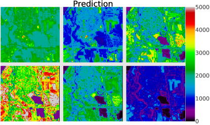
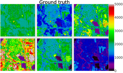
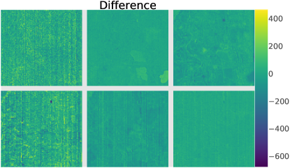
We tested our method also on data captured from Hyperion satellite [31] a sensor on board the satellite EO-1. The satellite carries a hyperspectral line scanner that records 242 channels (from 0.4 to 2.5 µm) at 30 m ground resolution, out of which 198 are calibrated and can be used. Our scenes are already cloud-free, have a size of $\approx$256$\times$7000 pixels, and show the river Rhine in Western Europe. Note, like most satellite data the images are stored with an intensity range of 16 bits ber channel, and have an effective radiometric depth of$\approx$5000 different gray values. The input image is emulated by integrating the hyper-spectral bands into the channels of ALI, the 9-channel multispectral sensor on board the same satellite. As test bed, we use different acquisitions dates over (roughly) the same area. This is of course a favourable scenario for our method: since training and test data show the same region, the network can learn adapt to the specific structure present in the region, and potentially to some degree even to the scene layout. Indeed, both the quantitative results in table 4 and the visual examples in Fig 6 validate the performance of our method over multiple visible and non-visible bands. While the training data is certainly favourable, it is not an unrealistic assumption that legacy hyper-spectral data for a given region is available. We find it quite remarkable that, according to the example, we are able to predict, with high accuracy, a finely resolved spectrum $>200$ bands from a standard, multi-spectral satellite image.

Figure 8: Adundances reconstruction from a satellite image. From top to bottom: input, our prediction, ground truth, tentative denoising over ground truth. Note how error free and well outlined are our abundances images w.r.t. the ground truth.

4.6 Denoising

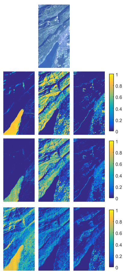
An interesting property of our learned upsampling is that it can be used as a denoising method: downsampling the original images (as we do in our experiments) removes noise, but upsampling does not re-insert it. Indeed it is known that deep neural networks achieve state-of-the-art results in image denoising [42]. See the prediction in Fig. 7, note how the marked line artifacts in the ground truth get removed by our method. On the satellite data, which is in general much noisier, this effect gets very prominent. In most of the cases the predicted images for Hyperion are cleaner and more useful than the original “ground truth” one. In Fig. 6 the difference images is dominated by the noise, while the “true” prediction error appears minimal. This claim is further supported by the fact that we were able to extract plausible spectral endmembers from the predicted hyperspectral images, which we found impossible for the originals.

4.7 Hyperspectral Unmixing

We also check our reconstruction on satellite data, by performing hyperspectral unmixing [5] a process that separates material information (also called endmembers) and their location in the image (also called abundances). We take an of the shelf endmember extraction algorithm (VCA, [27]) to identify dominant spectral signatures in the images. Then, we perform a Fully Constrained Least Squares (FCLS) adjustment to extract the abundance maps, according to the Linear Mixing Model (LMM) [19]. The abundance maps show the presence of each endmember in each pixel and are constrained to be non-negative and sum to one. We select a subset of one image and extract 15 endmembers and their corresponding abundances, for three different cases of hyperspectral image: Our prediction, ground truth and ground truth denoised, by projecting the data points onto the first 15 principal components of the image (PCA projection), see Fig 8. This kind of denoising method is suited for white noise as long as its variance is lower that that of the signal. Unfortunately, this is not enough to remove the noise from the abundance estimation, because the noise in this problem is not white, and so strong that apparently 15 principal components are insufficient to cover the underyling (obviously non-linear) subspace. As can be seen in Fig. 8 the ground truth itself cannot be used for hyperspectral unmixing as it is noisy. On the other hand, our method, only using 9 dimensions, is denoising the image as can be seen by the sharp abundance images, which clearly depict water, vegetation and urban areas, second row.

5 Conclusions

We show that it is possible to do super resolution for image not only in the spatial domain but also in the spectral domain. Our method builds on a recent high-performance convolutional neural network, which was originally designed for semantic segmentation. Contrary to other work on spectral super-resolution, we train and predict directly the end-to-end relation between an RGB image and its corresponding hyper-spectral image, without using any additional input, such as the spectral response function. We show the performance of our work on multiple indoor, outdoor and satellite datasets, where we compare favorably to other, less generic methods. We believe that our work may be useful for a number of applications that would benefit from higher spectral resolution, but where the recording conditions or the cost do not allow for routine use of hyper-spectral cameras.

References

- [1] N. Akhtar, F. Shafait, and A. Mian. Sparse spatio-spectral representation for hyperspectral image super-resolution. In European Conference on Computer Vision (ECCV), 2014.
- [2] N. Akhtar, F. Shafait, and A. Mian. Hierarchical beta process with gaussian process prior for hyperspectral image super resolution. In European Conference on Computer Vision, pages 103–120. Springer, 2016.
- [3] B. Arad and O. Ben-Shahar. Sparse recovery of hyperspectral signal from natural rgb images. In European Conference on Computer Vision, pages 19–34. Springer, 2016.
- [4] J. M. Bioucas-Dias, A. Plaza, G. Camps-Valls, P. Scheunders, N. M. Nasrabadi, and J. Chanussot. Hyperspectral remote sensing data analysis and future challenges. IEEE, Geoscience and Remote Sensing Magazine, 1(2):6–36, 2013.
- [5] J. M. Bioucas-Dias, A. Plaza, N. Dobigeon, M. Parente, Q. Du, P. Gader, and J. Chanussot. Hyperspectral unmixing overview: Geometrical, statistical, and sparse regression-based approaches. IEEE Journal of Selected Topics in Applied Earth Observations and Remote Sensing, 5(2):354–379, 2012.
- [6] G. Camps-Valls, D. Tuia, L. Bruzzone, and J. A. Benediktsson. Advances in hyperspectral image classification: Earth monitoring with statistical learning methods. IEEE Signal Processing Magazine, 31(1):45–54, 2013.
- [7] C. Chi, H. Yoo, and M. Ben-Ezra. Multi-spectral imaging by optimized wide band illumination. International Journal of Computer Vision, 86(2-3):140, 2010.
- [8] F. Chollet. Keras. https://github.com/fchollet/keras, 2015.
- [9] C. Dong, C. C. Loy, K. He, and X. Tang. Learning a deep convolutional network for image super-resolution. In European Conference on Computer Vision, pages 184–199. Springer, 2014.
- [10] W. Dong, L. Zhang, G. Shi, and X. Wu. Image deblurring and super-resolution by adaptive sparse domain selection and adaptive regularization. IEEE Transactions on Image Processing, 20(7):1838–1857, 2011.
- [11] T. Dozat. Incorporating nesterov momentum into adam. Technical report, Stanford University, Tech. Rep., 2015.[Online]. Available: http://cs229. stanford. edu/proj2015/054 report. pdf, 2015.
- [12] M. Elias and P. Cotte. Multispectral camera and radiative transfer equation used to depict leonardo’s sfumato in mona lisa. Applied optics, 47(12):2146–2154, 2008.
- [13] N. Gat. Imaging spectroscopy using tunable filters: a review. In AeroSense 2000, pages 50–64. International Society for Optics and Photonics, 2000.
- [14] K. He, X. Zhang, S. Ren, and J. Sun. Deep residual learning for image recognition. arXiv preprint arXiv:1512.03385, 2015.
- [15] K. He, X. Zhang, S. Ren, and J. Sun. Delving deep into rectifiers: Surpassing human-level performance on imagenet classification. In Proceedings of the IEEE international conference on computer vision, pages 1026–1034, 2015.
- [16] G. Huang, Z. Liu, K. Q. Weinberger, and L. van der Maaten. Densely connected convolutional networks. arXiv preprint arXiv:1608.06993, 2016.
- [17] S. Jégou, M. Drozdzal, D. Vazquez, A. Romero, and Y. Bengio. The one hundred layers tiramisu: Fully convolutional densenets for semantic segmentation. arXiv preprint arXiv:1611.09326, 2016.
- [18] R. Kawakami, Y. Matsushita, J. Wright, M. Ben-Ezra, Y.-W. Tai, and K. Ikeuchi. High-resolution hyperspectral imaging via matrix factorization. In Computer Vision and Pattern Recognition (CVPR), 2011 IEEE Conference on, pages 2329–2336. IEEE, 2011.
- [19] N. Keshava and J. F. Mustard. Spectral unmixing. IEEE signal processing magazine, 19(1):44–57, 2002.
- [20] J. Kim, J. Kwon Lee, and K. Mu Lee. Accurate image super-resolution using very deep convolutional networks. In The IEEE Conference on Computer Vision and Pattern Recognition (CVPR), June 2016.
- [21] J. Kim, J. Kwon Lee, and K. Mu Lee. Deeply-recursive convolutional network for image super-resolution. In The IEEE Conference on Computer Vision and Pattern Recognition (CVPR), June 2016.
- [22] S. J. Kim, F. Deng, and M. S. Brown. Visual enhancement of old documents with hyperspectral imaging. Pattern Recognition, 44(7):1461–1469, 2011.
- [23] D. Kingma and J. Ba. Adam: A method for stochastic optimization. arXiv preprint arXiv:1412.6980, 2014.
- [24] C. Lanaras, E. Baltsavias, and K. Schindler. Hyperspectral super-resolution by coupled spectral unmixing. In Proceedings of the IEEE International Conference on Computer Vision, pages 3586–3594, 2015.
- [25] G. Larsson, M. Maire, and G. Shakhnarovich. Learning representations for automatic colorization. In European Conference on Computer Vision, pages 577–593. Springer, 2016.
- [26] C. Ledig, L. Theis, F. Huszár, J. Caballero, A. Cunningham, A. Acosta, A. Aitken, A. Tejani, J. Totz, Z. Wang, et al. Photo-realistic single image super-resolution using a generative adversarial network. arXiv preprint arXiv:1609.04802, 2016.
- [27] J. Li and J. M. Bioucas-Dias. Minimum volume simplex analysis: A fast algorithm to unmix hyperspectral data. In Geoscience and Remote Sensing Symposium, 2008. IGARSS 2008. IEEE International, volume 3, pages III–250. IEEE, 2008.
- [28] R. M. Nguyen, D. K. Prasad, and M. S. Brown. Training-based spectral reconstruction from a single rgb image. In European Conference on Computer Vision, pages 186–201. Springer, 2014.
- [29] R. Padoan, T. A. Steemers, M. Klein, B. Aalderink, and G. De Bruin. Quantitative hyperspectral imaging of historical documents: technique and applications. Art Proceedings, pages 25–30, 2008.
- [30] Z. Pan, G. Healey, M. Prasad, and B. Tromberg. Face recognition in hyperspectral images. IEEE Transactions on Pattern Analysis and Machine Intelligence, 25(12):1552–1560, 2003.
- [31] J. S. Pearlman, P. S. Barry, C. C. Segal, J. Shepanski, D. Beiso, and S. L. Carman. Hyperion, a space-based imaging spectrometer. IEEE Transactions on Geoscience and Remote Sensing, 41(6):1160–1173, 2003.
- [32] W. Shi, J. Caballero, F. Huszar, J. Totz, A. P. Aitken, R. Bishop, D. Rueckert, and Z. Wang. Real-time single image and video super-resolution using an efficient sub-pixel convolutional neural network. In The IEEE Conference on Computer Vision and Pattern Recognition (CVPR), June 2016.
- [33] M. Simões, J. Bioucas-Dias, L. B. Almeida, and J. Chanussot. A convex formulation for hyperspectral image superresolution via subspace-based regularization. IEEE Transactions on Geoscience and Remote Sensing, 53(6):3373–3388, 2015.
- [34] I. Sutskever, J. Martens, G. E. Dahl, and G. E. Hinton. On the importance of initialization and momentum in deep learning. ICML (3), 28:1139–1147, 2013.
- [35] Y. Tarabalka, J. Chanussot, and J. A. Benediktsson. Segmentation and classification of hyperspectral images using watershed transformation. Pattern Recognition, 43(7):2367–2379, 2010.
- [36] R. Timofte, V. De Smet, and L. Van Gool. Anchored neighborhood regression for fast example-based super-resolution. In International Conference on Computer Vision (ICCV), 2013.
- [37] H. Van Nguyen, A. Banerjee, and R. Chellappa. Tracking via object reflectance using a hyperspectral video camera. In IEEE Computer Vision and Pattern Recognition Workshops (CVPRW), pages 44–51. IEEE, 2010.
- [38] Q. Wei, N. Dobigeon, and J.-Y. Tourneret. Fast fusion of multi-band images based on solving a sylvester equation. IEEE Transactions on Image Processing, 24(11):4109–4121, 2015.
- [39] D. Wu and D.-W. Sun. Advanced applications of hyperspectral imaging technology for food quality and safety analysis and assessment: A review—part i: Fundamentals. Innovative Food Science & Emerging Technologies, 19:1–14, 2013.
- [40] S. Wug Oh, M. S. Brown, M. Pollefeys, and S. Joo Kim. Do it yourself hyperspectral imaging with everyday digital cameras. In Proceedings of the IEEE Conference on Computer Vision and Pattern Recognition, pages 2461–2469, 2016.
- [41] E. Wycoff, T.-H. Chan, K. Jia, W.-K. Ma, and Y. Ma. A non-negative sparse promoting algorithm for high resolution hyperspectral imaging. In Acoustics, Speech and Signal Processing (ICASSP), 2013 IEEE International Conference on, pages 1409–1413. IEEE, 2013.
- [42] J. Xie, L. Xu, and E. Chen. Image denoising and inpainting with deep neural networks. In Advances in Neural Information Processing Systems, pages 341–349, 2012.
- [43] J. Yang, J. Wright, T. S. Huang, and Y. Ma. Image super-resolution via sparse representation. IEEE transactions on image processing, 19(11):2861–2873, 2010.
- [44] F. Yasuma, T. Mitsunaga, D. Iso, and S. Nayar. Generalized Assorted Pixel Camera: Post-Capture Control of Resolution, Dynamic Range and Spectrum. Technical report, Nov. 2008.
- [45] N. Yokoya, T. Yairi, and A. Iwasaki. Coupled nonnegative matrix factorization unmixing for hyperspectral and multispectral data fusion. IEEE Transactions on Geoscience and Remote Sensing, 50(2):528–537, 2012.
- [46] R. H. Yuhas, A. F. Goetz, and J. W. Boardman. Discrimination among semi-arid landscape endmembers using the spectral angle mapper (sam) algorithm. 1992.
- [47] R. Zeyde, M. Elad, and M. Protter. On single image scale-up using sparse-representations. In International conference on curves and surfaces, pages 711–730. Springer, 2010.
- [48] R. Zhang, P. Isola, and A. A. Efros. Colorful image colorization. In European Conference on Computer Vision, pages 649–666. Springer, 2016.