Continuous-time quantum Monte Carlo calculation of multi-orbital vertex asymptotics

Abstract

We derive the equations for calculating the high-frequency asymptotics of the local two-particle vertex function for a multi-orbital impurity model. These relate the asymptotics for a general local interaction to equal-time two-particle Green’s functions, which we sample using continuous-time quantum Monte Carlo simulations with a worm algorithm. As specific examples we study the single-orbital Hubbard model and the three $t_{2g}$ orbitals of SrVO₃ within dynamical mean field theory (DMFT). We demonstrate how the knowledge of the high-frequency asymptotics reduces the statistical uncertainties of the vertex and further eliminates finite box size effects. The proposed method benefits the calculation of non-local susceptibilities in DMFT and diagrammatic extensions of DMFT.

I Introduction

Strong electronic correlations are driving various properties of heavy fermion compounds, including Mott metal-to-insulator transitions, Mott (1968); Georges et al. (1996) magnetic phase transitions Löhneysen et al. (1994); Rohringer et al. (2011a), and quantum critical points. Schroder et al. (2000); Schäfer et al. (2016a) While Mott transitions can be described in terms of one-particle spectral functions only, the physics of the latter two is related to two-particle susceptibilities. Indeed, charge and magnetic susceptibilities are of primary interest when theoretical results are compared to experiments, but their computation in interacting systems is in general very costly. LeBlanc et al. (2015)

Typically, the Hubbard model Hubbard (1963) is employed when investigating strong electronic correlations from the theoretical side. This model has been solved successfully within the dynamical mean field theory (DMFT) Metzner and Vollhardt (1989); Georges and Kotliar (1992); Kotliar and Vollhardt (2004); Held (2007) which corresponds to a purely local self-energy. For determining this local self-energy, DMFT maps the Hubbard model onto an auxiliary single-impurity Anderson model (AIM), Anderson (1961) which can be solved numerically. Nowadays, a vast amount of impurity solvers exist, each having its particular strengths and weaknesses.Hirsch and Fye (1986); Sakai et al. (2006); Bulla et al. (2008); Karski et al. (2008); Ganahl et al. (2014); Caffarel and Krauth (1994); Zgid et al. (2012) A noteworthy group of impurity solvers includes the continuous-time quantum Monte Carlo (CT-QMC) methods, which can treat impurities with many degrees of freedom, general interactions, and continuous bath dispersions. Rubtsov and Lichtenstein (2004); Werner et al. (2006); Werner and Millis (2006); Gull et al. (2008, 2011) These algorithms are capable of calculating finite-temperature correlation functions (i.e. one- and two-particle Green’s functions), which directly relate to the aforementioned susceptibilities and to vertex functions, respectively.

While DMFT is exact in infinite spatial dimensions, the theory is often used as an approximation for finite dimensional systems. In this case, correlations that are non-local in space may emerge. There are several approaches which contain the local DMFT correlations but extend it for also including non-local ones. The extensions of DMFT are grouped into cluster methods, which enlarge the AIM to multiple impurities or, alternatively, methods which diagrammatically improve upon DMFT. Promising diagrammatic extensions in this context include the dynamic vertex approximation ($\mathrm{D}\Gamma\mathrm{A}$), Toschi et al. (2007) the dual fermion method (DF), Rubtsov et al. (2008) the one-particle irreducible approach (1PI), Rohringer et al. (2013) the DMFT to functional renormalization group ($\mathrm{DMF}^{2}\mathrm{RG}$)Taranto et al. (2014) and the quadruply irreducible local expansion (QUADRILEX).Ayral and Parcollet (2016) Although these methods follow in general quite different philosophies, they all rely on the knowledge of the local two-particle susceptibility or vertex function. These vertex functions have two incoming and two outgoing lines so that they depend on three frequencies [exploiting energy conservation] and two spin combinations [exploiting SU(2) symmetry].Rohringer et al. (2012) For multi-orbital calculations there are, on top of this, various combinations of the orbital degrees of freedom.

Albeit in principle straight-forward, it is a very challenging task to extract the local multi-orbital two-particle-susceptibility of the AIM within large frequency-boxes. This can be traced back to the high computational resources in computing, storing and processing the two-particle object. Only recently the local two-particle correlation function with its complete frequency structure was obtained for SrVO₃ with SU(2)-symmetric interaction. Galler et al. (2017) In order to overcome this limitation, contemporary attempts include approximating the asymptotic frequency behavior. The two main pieces of work in this direction are: (i) extracting the high-frequency asymptotics of the local two-particle vertex function $\Gamma_{ph}$ that is irreducible in the particle-hole channel by approximating it by a certain sub-class of single-frequency susceptibility functions, Kuneš (2011) (ii) extracting the complete high-frequency asymptotics of the full vertex $F$ through all asymptotically contributing diagrams within the so-called kernel approximations, which include one and two-frequency kernel functions. Li et al. (2016); Wentzell et al. While (ii) is not limited to a specific sub-class of diagrams (i.e. particle-hole, particle-particle …) and yields the full asymptotics of the vertex, the derivation currently only exists for the single-orbital case. Approach (i), on the other hand, was implemented for multi-orbital systems in Ref. Kuneš, 2011, and successfully applied for calculating the $\omega=0$ susceptibility in DMFT, but not for generalized susceptibilities or diagrammatic extensions of DMFT. For calculating $\Gamma_{ph}$, Ref. Kuneš, 2011 also introduced an efficient implementation of the inversion of the Bethe-Salpeter equation. This has been extended to arbitrary channels and $\omega\neq 0$ in Ref. Tagliavini et al., 2017.

In this paper we will follow approach (ii) in order to avoid divergences in the local two-particle irreducible vertex function Schäfer et al. (2013); Schäfer et al. (2016b) and further to include all local physics by considering all relevant diagrams. Since the kernel approximations are originally formulated for the vertex function instead of the susceptibility or correlation function, in this work we outline how to extract the kernel approximations from the correlation functions. Prior to this work, the kernel functions were approximated from the local two-particle vertex function itself by scanning the asymptotic region and employing this information for the functional renormalization group (fRG) flow Wentzell et al. and for the self-consistent solution of the parquet equations Li et al. (2016). This approach is not suitable for quantum Monte Carlo algorithms due to the intrinsic statistical uncertainty. Here, we demonstrate a method which directly allows us to measure the correlation functions related to the kernel functions with impurity solvers, such as CT-QMC or, in principle, any other type of impurity solver that is based on a Green’s function formalism. We further extend the kernel approximations by deriving the expressions for multi-orbital systems with general local interactions.

Let us emphasize that the hybridization expansion (CT-HYB) Werner and Millis (2006) is the method of choice when dealing with the multi-orbital AIM at finite temperature and non-density-density interaction. We use a worm algorithm recently introduced to CT-HYB, Gunacker et al. (2015, 2016) to measure one- and two-time two-particle correlation functions, which are then transformed into the kernel functions. Combining the sampling power of CT-HYB with the improvements due to the asymptotical structure allows us to access local physics of multi-orbital systems and especially of materials with strongly reduced statistical uncertainty.

In Section II we present the theoretical foundation required for a rigorous definition of the multi-orbital kernel approximations. Starting from the two-particle Green’s function, we define the correlation functions, the susceptibilities and the vertex functions. We further define the concepts of reducibility and irreducibility of two-particle quantities, respectively. We show the local formulation of the parquet equations and the necessary frequency representations. In order to establish the connection between correlation functions and kernel approximations, we define in Section III the equal-time susceptibilities and the corresponding multi-orbital kernel approximations. We further define the parameterization of the asymptotical structure and its connection to the full vertex function. We briefly present what modifications of the worm algorithm are necessary in Section IV, analyze the numerical effort, and present a summary of the steps needed to calculate the Kernel functions. In Section V we apply the method to the single-orbital Hubbard model and benchmark our approach against results obtained from exact diagonalization (ED). In a second step, we show results for the multi-orbital case, by calculating the asymptotical structure of SrVO₃, and outline the improvement with respect to the direct measurement of the two-particle correlation function. In Section VI we summarize our method in terms of its strengths and its prospective applications. Our frequency conventions and additional derivations for the atomic limit are given in the Appendix.

II Hamiltonian and theoretical background

In this paper, we consider the multi-orbital AIM (which in DMFT is calculated self-consistently Georges et al. (1996); Held (2007)):

$$H=\frac{1}{4}\sum_{ijkl}U_{ijkl}^{\vphantom{dagger}}d^{\dagger}_{i}d^{\dagger}_{j}d^{\vphantom{dagger}}_{l}d^{\vphantom{dagger}}_{k}+\sum_{i}\tilde{\varepsilon}^{\vphantom{dagger}}_{i}d_{i}^{\dagger}d_{i}^{\vphantom{dagger}}+\\ +\sum_{Ki}\varepsilon^{\vphantom{dagger}}_{Ki}c^{\dagger}_{Ki}c^{\vphantom{dagger}}_{Ki}+\sum_{Kij}\left[V_{K}^{ij}c^{\dagger}_{Ki}d^{\vphantom{dagger}}_{j}+(V_{K}^{ji})^{*}d^{\dagger}_{i}c^{\vphantom{dagger}}_{Kj}\right]\;$$ (1)

Here, $d_{i}$ ($d_{i}^{\dagger}$) is the annihilation (creation) operator of a fermion with spin-orbital flavor $i$, $c_{Ki}$ ($c_{Ki}^{\dagger}$) is the annihilation (creation) operator of an electron with impurity flavor $i$ in the non-interacting bath and $K$ sums over the remaining bath degrees of freedom (e. g. the momentum $\mathbf{k}$). The local impurity is described by a local one-particle potential $\tilde{\varepsilon}_{i}$ (e.g. the crystal field), the fully anti-symmetrized interaction matrix $U_{ijkl}$, the bath dispersion $\varepsilon_{Ki}$, and the hybridization strength $V_{K}^{ij}$.

The $n$-particle Green’s function of a local impurity in imaginary-time reads:

$$G_{i_{1}i_{2}\ldots i_{2n-1}i_{2n}}(\tau_{1},\tau_{2},\ldots,\tau_{2n-1},\tau_{2n})=\\ (-1)^{n}\langle T_{\tau}d^{\vphantom{dagger}}_{i_{1}}(\tau_{1})d_{i_{2}}^{\dagger}(\tau_{2})\ldots d^{\vphantom{dagger}}_{i_{2n-1}}(\tau_{2n-1})d_{i_{2n}}^{\dagger}(\tau_{2n})\rangle,$$ (2)

where $d_{i}(\tau_{i})$ ($d_{i}^{\dagger}(\tau_{i})$) are now the imaginary-time dependent annihilation (creation) operators at (imaginary) time $\tau_{i}$. Further, $T_{\tau}$ is the imaginary-time ordering operator, and $\langle\ldots\rangle=(\text{Tr}e^{\beta H}\ldots)/Z$ the thermal expectation value at temperature $T$ ($\beta=1/T$), $Z$ is the partition function. Expanding  Eq. (2) into a perturbation series and decomposing it according to Wick’s theorem yields all possible connected and disconnected Feynman diagrams. Distinguishing between disconnected and connected diagrams allows us to classify the $n$-particle Green’s function into the $2n$-point correlation function and the subset of connected diagrams into $n$-particle vertex function.

At the two-particle level the Green’s function decomposes into two disconnected parts, usually referred to as straight and cross terms, and a fully connected part:

$$G_{ijkl}(\tau_{1},\tau_{2},\tau_{3},\tau_{4})=G_{ij}(\tau_{1},\tau_{2})G_{kl}(\tau_{3},\tau_{4})\\ \underbrace{-G_{il}(\tau_{1},\tau_{4})G_{kj}(\tau_{2},\tau_{3})+\chi^{\text{c}}_{ijkl}(\tau_{1},\tau_{2},\tau_{3},\tau_{4})}_{\equiv\chi_{ijkl}}.$$ (3)

The cross term and the connected diagrams are further grouped into the generalized 4-point susceptibility $\chi_{ijkl}$.

Figure 1: Decomposition of the two-particle Green’s function into disconnected parts and a connected part.

The two-particle vertex function $F_{mnop}$ now follows from the subset of connected diagrams by amputating the outer legs (one-particle Green’s functions):

$$\chi^{\text{c}}_{ijkl}(\tau_{1},\tau_{2},\tau_{3},\tau_{4})=-\,\,\,\mathclap{\displaystyle\int}\mathclap{\textstyle\sum}\;\;\;G_{im}(\tau_{1},\tau_{5})G_{nj}(\tau_{6},\tau_{2})\times\\ F_{mnop}(\tau_{5},\tau_{6},\tau_{7},\tau_{8})G_{ko}(\tau_{3},\tau_{7})G_{pl}(\tau_{8},\tau_{4}),$$ (4)

where we integrate/sum over all internal imaginary time/spin-orbital degrees of freedom. That is, the $n$-particle vertex functions are defined without outer legs, whereas $n$-particle Green’s functions and $2n$-point susceptibilities are defined with outer legs attached.

For any two-particle object considered in the following it is often useful to consider the Matsubara frequency representation, instead of the imaginary-time representation:

$$\mathcal{A}^{\nu_{1}\nu_{2}\nu_{3}\nu_{4}}_{ijkl}=\int_{0}^{\beta}\mathrm{d}\tau_{1}\mathrm{d}\tau_{2}\mathrm{d}\tau_{3}\mathrm{d}\tau_{4}\times\\ e^{i(\nu_{1}\tau_{1}-\nu_{2}\tau_{2}+\nu_{3}\tau_{3}-\nu_{4}\tau_{4})}\mathcal{A}_{ijkl}(\tau_{1},\tau_{2},\tau_{3},\tau_{4}),$$ (5)

where $\mathcal{A}\in\{G,\chi,F\}$ and $\nu_{i}=(2n+1)\pi/\beta$ are the discrete fermionic Matsubara frequencies. The decomposition of the correlation function into disconnected parts and a fully connected part in Matsubara frequencies is illustrated in Fig. 1. The back-transform is defined as:

$$\mathcal{A}_{ijkl}(\tau_{1},\tau_{2},\tau_{3},\tau_{4})=\frac{1}{\beta^{4}}\times\\ \sum_{\nu_{1},\nu_{2},\nu_{3},\nu_{4}}e^{-i(\nu_{1}\tau_{1}-\nu_{2}\tau_{2}+\nu_{3}\tau_{3}-\nu_{4}\tau_{4})}\mathcal{A}^{\nu_{1}\nu_{2}\nu_{3}\nu_{4}}_{ijkl}.$$ (6)

When setting a single time-argument to zero only the frequency summation (without the exponential function) remains. This already implies that contracting two legs by a Matsubara frequency sum relates to setting the respective time differences to zero (which usually appear in mixed bosonic-fermionic frequency representations) thus resulting in an equal-time object.

The time-translational symmetry inherent to the $n$-particle Green’s function in imaginary time converts to an energy conservation in Matsubara frequency space.

$$\nu_{1}+\nu_{3}=\nu_{2}+\nu_{4}$$ (7)

Consequently, it is sometimes more useful to assume a mixed bosonic-fermionic frequency representation with two fermionic and one bosonic frequency. Each reducible channel introduced in the next section has its own natural frequency representation. The mapping between the four-frequency notation and the three-frequency notation that is natural in each channel is given in the Appendix A.

When considering vertex functions in terms of Feynman diagrams it is useful to define the concept of reducibility. Here, $n=1,2$-particle irreducible means that the vertex cannot be separated into two or more parts by cutting $n$ Green’s function lines. At the one-particle level, the one-particle irreducible vertex can be obtained from the Dyson equation and is usually referred to as self-energy $\Sigma$. At the two-particle level, it is necessary to consider reducibility more carefully. The two-particle vertex function $F$ is one-particle irreducible, however, it is not two-particle irreducible.

The (local) Parquet equations De Dominicis (1962); De Dominicis and Martin (1964); Bickers (2004)decompose the two-particle vertex function $F$ into irreducible and reducible components:

$$F_{ijkl}=\Lambda_{ijkl}+\Phi^{ph}_{ijkl}+\Phi^{\mkern 1.5mu\overline{\mkern-1.5muph\mkern-1.5mu}\mkern 1.5mu}_{ijkl}+\Phi^{pp}_{ijkl},$$ (8)

where $\Lambda$ is the fully two-particle irreducible vertex function, and $\Phi^{ph},\Phi^{\mkern 1.5mu\overline{\mkern-1.5muph\mkern-1.5mu}\mkern 1.5mu},\Phi^{pp}$ are the two-particle reducible vertex in the particle-hole ($ph$), the particle-hole transversal ($\mkern 1.5mu\overline{\mkern-1.5muph\mkern-1.5mu}\mkern 1.5mu$) and the particle-particle ($pp$) channel. In Eq. (8) we have omitted the time/frequency dependence of each quantity. The subset of two-particle irreducible diagrams in a given channel $\ell=\{ph,\mkern 1.5mu\overline{\mkern-1.5muph\mkern-1.5mu}\mkern 1.5mu,pp\}$ is acquired by subtracting the reducible diagrams from the full vertex $F$, i. e.

$$\Gamma^{\ell}_{ijkl}=F_{ijkl}-\Phi^{\ell}_{ijkl}.$$ (9)

Constructing the reducible vertex functions as ladders leads to the Bethe-Salpeter equation

$$\Gamma^{\ell}=F-\int\Gamma^{\ell}(GG)^{\ell}F.$$ (10)

The asymptotic form of the two-particle irreducible vertex in the $ph$-channel is calculated elsewhere, Kuneš (2011) we focus on the full vertex $F$.

III Asymptotical structure of the local vertex

III.1 Motivation

In the following we derive the high-frequency asymptotics of the full two-particle vertex function $F$. Alternatively, and in a very similar manner, one may derive the asymptotical behavior of the two-particle Green’s function or the generalized susceptibility. The former, however, is superior, because contrary to the susceptibility, the vertex can be parameterized very efficiently in its high-frequency region.
In order to describe this high-frequency asymptotics, we reiterate that outside of the low-frequency region only one contribution, the constant background, originates from the two-particle-irreducible vertex $\Lambda$.Wentzell et al. ; Rohringer et al. (2012) The remaining high-frequency-structures are contained in the vertices $\Phi^{\ell}$ reducible in channel $\ell$ and can be parameterized through much simpler one- and two-frequency objects, coined Kernel-1 and Kernel-2 functions.Wentzell et al. ; Rohringer et al. (2012) The constant background can be identified as the bare vertex $U_{abcd}$ shown in Fig. 2, which is the lowest-order term in the diagrammatic series for the full vertex.

Next, we have the Kernel-1 diagrams that only depend on one bosonic frequency and are depicted in Fig. 3. Here, two pairs of (incoming or outgoing) lines enter at the respective same interaction $U$. In this case the vertex depends only on the total transferred frequency at these interactions (it is the same bosonic frequency for both pairs because of energy conservation).Wentzell et al. ; Rohringer et al. (2012) There are three diagrams in Fig. 3 and hence there are three Kernel-1 contributions each of which depends on a single bosonic frequency. Switching from Matsubara frequencies to imaginary times, as defined in Eq. (6), it turns out that the dependence on frequency differences corresponds to diagrams with pairwise equal times. That is, the diagrams shown in Fig. 3 correspond to the summation of all terms with two equal-time pairs.

For the Kernel-2 diagrams of Fig. 4, we have only one pair of external legs that enter at the same $U$. Hence such diagrams depend on the transferred bosonic frequency at this $U$ and (because of energy conservation) one additional fermionic frequency of the unpaired legs. This corresponds to one equal-time pair in Fourier space. All the diagrams Fig. 3 and Fig. 4 are two-particle reducible and thus, the asymptotic form of the full vertex $F$ consists, apart from the constant background $U$, only of reducible terms $\Phi^{\ell}_{asympt}$.

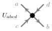
Figure 2: Diagram of the bare local interaction $U$. The bare vertex does not contain any Green’s function, the (amputated) legs drawn in gray indicate the direction of the incoming/outgoing particles and their spin-orbital flavor $a,b,c,d$ (the Matsubara frequencies are suppressed for simplicity).

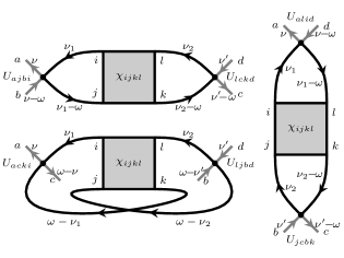
Figure 3: Vertex diagrams that depend on only one bosonic frequency, in $ph$-channel (top left), $\mkern 1.5mu\overline{\mkern-1.5muph\mkern-1.5mu}\mkern 1.5mu$-channel (right) and $pp$-channel (bottom left). Frequencies are given in the channel-specific notation (see Appendix A).

Figure 4: Vertex diagrams that depend on one bosonic and one fermionic frequency, in $ph$-channel (top left), $\mkern 1.5mu\overline{\mkern-1.5muph\mkern-1.5mu}\mkern 1.5mu$-channel (right) and $pp$-channel (bottom left). Frequencies are given in the channel-specific notation (see Appendix A).

III.2 Equal-time two-particle Green’s functions

We now have to find a way to extract the aforementioned asymptotics from Green’s function-like quantities, which are accessible in impurity solvers such as CT-QMC.

Considering the full Green’s function $G_{ijkl}(\tau_{1},\tau_{2},\tau_{3},\tau_{4})$, we need to form two equal-time pairs for the diagrams of Fig. 3 to arrive at a function of two time arguments or one frequency-difference. There are three distinct ways to achieve this:

$$\tau_{1}=\tau_{2}\equiv\tau,\;\tau_{3}=\tau_{4}\equiv\tau^{\prime}$$ (11)

$$\tau_{1}=\tau_{3}\equiv\tau,\;\tau_{2}=\tau_{4}\equiv\tau^{\prime}$$ (12)

$$\tau_{1}=\tau_{4}\equiv\tau,\;\tau_{2}=\tau_{3}\equiv\tau^{\prime}$$ (13)

which relate to the $ph$, $pp$ and $\mkern 1.5mu\overline{\mkern-1.5muph\mkern-1.5mu}\mkern 1.5mu$ channel. The “two-legged” two-particle Green’s function for the $ph$-channel, defined in (11), is

$$G^{ph,\nu_{1}-\nu_{2}}_{ijkl}=\int\mathrm{d}\tau\mathrm{d}\tau^{\prime}e^{i(\nu_{1}-\nu_{2})(\tau-\tau^{\prime})}\times\\ \langle T_{\tau}d_{i}(\tau)d^{\dagger}_{j}(\tau)d_{k}(\tau^{\prime})d^{\dagger}_{l}(\tau^{\prime})\rangle,$$ (14)

and for the $pp$-channel, we get

$$G^{pp,\nu_{1}+\nu_{3}}_{ijkl}=\int\mathrm{d}\tau\mathrm{d}\tau^{\prime}e^{i(\nu_{1}+\nu_{3})(\tau-\tau^{\prime})}\times\\ \langle T_{\tau}d_{i}(\tau)d^{\dagger}_{j}(\tau^{\prime})d_{k}(\tau)d^{\dagger}_{l}(\tau^{\prime})\rangle.$$ (15)

While the above functions have to be measured separately, the third, related to the $\mkern 1.5mu\overline{\mkern-1.5muph\mkern-1.5mu}\mkern 1.5mu$-channel, can be obtained from the first by the crossing relation (see Ref. Galler et al., 2017 for an illustration)

$$G^{\mkern 1.5mu\overline{\mkern-1.5muph\mkern-1.5mu}\mkern 1.5mu}_{ijkl}=-G^{ph}_{ilkj}$$ (16)

and depends on the frequency difference $\nu_{1}-\nu_{4}$.

From the six ways to form one equal-time pair as needed for the diagrams Fig. 4, it is sufficient to consider only the following three, with the others related by time-reversal symmetry:

$$\tau_{1}\equiv\tau,\;\tau_{2}\equiv\tau^{\prime},\;\tau_{3}=\tau_{4}\equiv\tau^{\prime\prime},$$ (17)

$$\tau_{1}\equiv\tau,\;\tau_{3}\equiv\tau^{\prime},\;\tau_{2}=\tau_{4}\equiv\tau^{\prime\prime},$$ (18)

$$\tau_{1}\equiv\tau,\;\tau_{4}\equiv\tau^{\prime},\;\tau_{2}=\tau_{3}\equiv\tau^{\prime\prime}.$$ (19)

Here, Eqs. (17)-(19) are related, as before, to the $ph$, $pp$ and $\mkern 1.5mu\overline{\mkern-1.5muph\mkern-1.5mu}\mkern 1.5mu$ channel. The “three-legged” two-particle Green’s function in the $ph$-channel corresponding to Eq. (17) follows as

$$G^{ph,\nu_{1},\nu_{1}-\nu_{2}}_{ijkl}=\int\!\!\mathrm{d}\tau\mathrm{d}\tau^{\prime}\mathrm{d}\tau^{\prime\prime}e^{i(\nu_{1}(\tau-\tau^{\prime})+(\nu_{1}-\nu_{2})(\tau^{\prime}\!-\tau^{\prime\prime}))}\times\\ \langle T_{\tau}d_{i}(\tau)d^{\dagger}_{j}(\tau^{\prime})d_{k}(\tau^{\prime\prime})d^{\dagger}_{l}(\tau^{\prime\prime})\rangle,$$ (20)

and in the $pp$-channel (Eq. (18)) it is

$$G^{pp,\nu_{1},\nu_{1}+\nu_{3}}_{ijkl}=\int\!\!\mathrm{d}\tau\mathrm{d}\tau^{\prime}\mathrm{d}\tau^{\prime\prime}e^{i(\nu_{1}(\tau-\tau^{\prime})+(\nu_{1}+\nu_{3})(\tau^{\prime}\!-\tau^{\prime\prime}))}\times\\ \langle T_{\tau}d_{i}(\tau)d^{\dagger}_{j}(\tau^{\prime\prime})d_{k}(\tau^{\prime})d^{\dagger}_{l}(\tau^{\prime\prime})\rangle.$$ (21)

Again, the Green’s function in the $\mkern 1.5mu\overline{\mkern-1.5muph\mkern-1.5mu}\mkern 1.5mu$-channel can be obtained by the crossing relation Eq. (16), the frequency arguments are then $\nu_{1}$ and $\nu_{1}-\nu_{4}$. Please note that $\nu_{1}-\nu_{2}$, $\nu_{1}+\nu_{3}$ and $\nu_{1}-\nu_{4}$ are referred to as the channel-specific bosonic Matsubara frequencies $\omega_{ph}$, $\omega_{pp}$ and $\omega_{\mkern 1.5mu\overline{\mkern-1.5muph\mkern-1.5mu}\mkern 1.5mu}$, respectively. A full table with channel-specific frequency notations is given in Appendix A.

III.3 Subtraction of disconnected parts

We have seen in Eq. (3) and Fig. 1, that the full two-particle Green’s function, as measured in CT-QMC, contains one connected and also two disconnected parts. Hence, in order to arrive at the two- and three-legged diagrams of Fig. 3 and Fig. 4, it is necessary to eliminate the disconnected terms. In the following we will assume the one-particle Green’s function to be flavor diagonal, such that $G_{ij}(\tau_{1},\tau_{2})\equiv G_{i}(\tau_{1},\tau_{2})\delta_{ij}$. We recover the physical single-frequency susceptibility in the particle-hole channel by subtracting the constant “straight term”,

$$\chi_{ijkl}^{ph,\omega}=G_{ijkl}^{ph,\omega}-(1-n_{i})(1-n_{k})\delta_{\omega 0}\delta_{ij}\delta_{kl},$$ (22)

whereas the particle-particle susceptibility is already given by

$$\chi_{ijkl}^{pp,\omega}=G_{ijkl}^{pp,\omega}.$$ (23)

We will now turn to the three-legged Green’s functions, where we are again interested only in the connected part corresponding to Fig. 4. For the particle-hole channel we find

$$\chi^{\text{c},ph,\nu\omega}_{ijkl}=G^{ph,\nu\omega}_{ijkl}-G_{i}^{\nu}\times\\ \left[(n_{k}-1)\delta_{ij}\delta_{kl}\delta_{\omega 0}-G_{k}^{\nu-\omega}\delta_{il}\delta_{jk}\right]$$ (24)

and for the particle-particle channel

$$\chi^{\text{c},pp,\nu\omega}_{ijkl}=G^{pp,\nu\omega}_{ijkl}-\left(\delta_{ij}\delta_{kl}-\delta_{il}\delta_{jk}\right)G_{i}^{\nu}G_{k}^{\omega-\nu}.$$ (25)

As usual, the corresponding expressions for the transverse particle-hole channel can be obtained by applying the crossing relation Eq. (16).

III.4 Kernel functions

After the subtraction of the disconnected parts from the two-particle Green functions, the next step is to contract the equal-time legs with interaction vertices. The two-legged objects have two pairs of equal times and therefore need two distinct bare vertices to contract their legs and obtain the Kernel-1 functions $K^{(1),\ell}$:

$$K^{(1),ph,\omega}_{abcd} =-\sum_{ijkl}U_{ajbi}\,\chi_{ijkl}^{ph,\omega}\,U_{lckd}$$ (26)

$$K^{(1),\mkern 1.5mu\overline{\mkern-1.5muph\mkern-1.5mu}\mkern 1.5mu,\omega}_{abcd} =-\sum_{ijkl}U_{alid}\,\chi_{ijkl}^{\mkern 1.5mu\overline{\mkern-1.5muph\mkern-1.5mu}\mkern 1.5mu,\omega}\,U_{jcbk}$$ (27)

$$K^{(1),pp,\omega}_{abcd} =-\sum_{ijkl}\frac{U_{acki}}{2}\,\chi_{ijkl}^{pp,\omega}\,\frac{U_{ljbd}}{2}$$ (28)

This corresponds precisely to the diagrams shown in Fig. 3.

For the Kernel-2 approximations, the procedure is a bit more involved. After the bare vertex contraction, we need to amputate the remaining legs. Thus, the Kernel-2 functions $K^{(2),\ell}$ in all three channels are

$$K^{(2),ph,\nu\omega}_{abcd} =\sum_{ij}\frac{-\chi^{\text{c},ph,\nu\omega}_{abji}}{G_{a}^{\nu}G_{b}^{\nu-\omega}}\,U_{icjd}-K^{(1),ph,\omega}_{abcd}$$ (29)

$$K^{(2),\mkern 1.5mu\overline{\mkern-1.5muph\mkern-1.5mu}\mkern 1.5mu,\nu\omega}_{abcd} =\sum_{ij}\frac{-\chi^{\text{c},\mkern 1.5mu\overline{\mkern-1.5muph\mkern-1.5mu}\mkern 1.5mu,\nu\omega}_{aijd}}{G_{a}^{\nu}G_{d}^{\nu-\omega}}\,U_{icbj}-K^{(1),\mkern 1.5mu\overline{\mkern-1.5muph\mkern-1.5mu}\mkern 1.5mu,\omega}_{abcd}$$ (30)

$$K^{(2),pp,\nu\omega}_{abcd} =\sum_{ij}\frac{-\chi^{\text{c},pp,\nu\omega}_{aicj}}{G_{a}^{\nu}G_{c}^{\nu-\omega}}\,\frac{U_{jibd}}{2}-K^{(1),pp,\omega}_{abcd},$$ (31)

where we had to subtract the Kernel-1 functions in order to avoid double-counting of diagrams.

Now we have six functions going to zero for high frequencies $\nu$ or $\omega$, from which we can compile the asymptotic vertex.

III.5 Asymptotic form of the full vertex

According to the (local) parquet equation, the full vertex $F_{abcd}$ can be decomposed into a fully irreducible and several reducible parts:

$$F_{abcd}^{\nu\nu^{\prime}\omega}=\Lambda_{abcd}^{\nu\nu^{\prime}\omega}+\Phi_{abcd}^{ph,\nu\nu^{\prime}\omega}+\Phi_{abcd}^{\mkern 1.5mu\overline{\mkern-1.5muph\mkern-1.5mu}\mkern 1.5mu,\nu\nu^{\prime}\omega}+\Phi_{abcd}^{pp,\nu\nu^{\prime}\omega}.$$ (32)

We are now able to construct the asymptotic form of the reducible vertices $\Phi$ using:Wentzell et al.

$$\Phi^{\text{asympt},\ell,\nu\nu^{\prime}\omega}_{abcd}=K^{(1),\ell,\omega}_{abcd}+K^{(2),\ell,\nu\omega}_{abcd}+\mkern 1.5mu\overline{\mkern-1.5muK\mkern-1.5mu}\mkern 1.5mu^{(2),\ell,\nu^{\prime}\omega}_{abcd},$$ (33)

where the functions $\mkern 1.5mu\overline{\mkern-1.5muK\mkern-1.5mu}\mkern 1.5mu^{(2),\ell}$ are found to be equal to $K^{(2),\ell}$ due to time-reversal symmetry. Therefore summing up all $K^{(i),\ell}$, we get the asymptotic form of the full vertex:

$$F^{\text{asympt}}_{abcd}(\nu_{\ell},\nu_{\ell}^{\prime},\omega_{\ell})-U_{abcd}=\\ K^{(1),ph,\omega_{ph}}_{abcd}+K^{(2),ph,\nu_{ph}\omega_{ph}}_{abcd}+K^{(2),ph,\nu^{\prime}_{ph}\omega_{ph}}_{abcd}\\ +K^{(1),\mkern 1.5mu\overline{\mkern-1.5muph\mkern-1.5mu}\mkern 1.5mu,\omega_{\mkern 1.5mu\overline{\mkern-1.5muph\mkern-1.5mu}\mkern 1.5mu}}_{abcd}+K^{(2),\mkern 1.5mu\overline{\mkern-1.5muph\mkern-1.5mu}\mkern 1.5mu,\nu_{\mkern 1.5mu\overline{\mkern-1.5muph\mkern-1.5mu}\mkern 1.5mu}\omega_{\mkern 1.5mu\overline{\mkern-1.5muph\mkern-1.5mu}\mkern 1.5mu}}_{abcd}+K^{(2),\mkern 1.5mu\overline{\mkern-1.5muph\mkern-1.5mu}\mkern 1.5mu,\nu^{\prime}_{\mkern 1.5mu\overline{\mkern-1.5muph\mkern-1.5mu}\mkern 1.5mu}\omega_{\mkern 1.5mu\overline{\mkern-1.5muph\mkern-1.5mu}\mkern 1.5mu}}_{abcd}\\ +K^{(1),pp,\omega_{pp}}_{abcd}+K^{(2),pp,\nu_{pp}\omega_{pp}}_{abcd}+K^{(2),pp,\nu^{\prime}_{pp}\omega_{pp}}_{abcd}$$ (34)

In this way we are now able to build arbitrarily large vertices in any frequency notation, which leads to significant improvements of further calculations.

IV Implementation

IV.1 Worm Sampling

For the calculation of the equal-time two-particle Green’s functions we employ the hybridization expansion (CT-HYB) Werner and Millis (2006) due to its favorable scaling at finite temperature and its ability to treat general local interactions efficiently. The traditional formulation of the CT-HYB algorithm assumes importance sampling and explores the phase space of the partition function $Z$. One- and two-particle Green’s function are then obtained by “removing” hybridization lines. For non-density-density interactions, this is in general not possible. Instead, we hence use a worm algorithm recently introduced to CT-HYB, Gunacker et al. (2015, 2016) and measure equal-time two-particle correlation functions, which are then transformed into the kernel functions (26) - (31) in a post-processing step.

Worm sampling stands in contrast to partition function sampling as we no longer explore the phase space $\mathcal{C}_{Z}$ of the partition function, but rather an extended phase space $\mathcal{C}_{W}$ for an extended partition function ${W=Z+\eta Z_{G}}$, where $Z_{G}$ is the partition function of an exemplary worm space and $\eta$ the relative balancing factor. While we sample configurations, which do not represent the denominator of the expectation value, we profit due to more flexibility in defining the estimator. The exact procedure on how to define equal-time Green’s function estimators can be found in previous works. Gunacker et al. (2016) By adding the local creation and annihilation operators of the estimators to the local trace of the infinite perturbation series in the hybridization expansion, one effectively switches to worm space. We redefine the single-frequency expectation values in Eqs. (14)-(15) in terms of worm estimators:

$$G^{\ell,\omega}_{\mathcal{C}_{1,\ell}}=\langle\mathrm{sgn}\times e^{i\omega(\tau-\tau^{\prime})}\rangle_{MC},$$ (35)

where $\mathcal{C}_{1,\ell}$ are the configuration spaces of the particle-hole and particle-particle single-frequency estimator and ‘sgn’ denotes the sign of the configuration. Further, the two-frequency expectation values in Eqs. (20)-(21) follow as:

$$G^{\ell,\nu\omega}_{\mathcal{C}_{2,\ell}}=\langle\mathrm{sgn}\times e^{i(\nu(\tau-\tau^{\prime})+\omega(\tau^{\prime}-\tau^{\prime\prime}))}\rangle_{MC},$$ (36)

where $\mathcal{C}_{2,\ell}$ are the configuration spaces of the particle-hole and particle-particle two-frequency estimator. We emphasize that the measured quantities still need to be normalized with respect to the partition function.

Apart from the above estimators assuming $\delta$-like bins, we have further implemented estimators considering the entire configuration as suggested in Ref. Shinaoka et al., 2017. At this point we note that for density-density interactions the worm algorithm is not necessary. Instead an implementation of the estimators in a segment algorithm is more feasible. In another context, the three-legged estimator was already defined for the segment representation. Hafermann (2014)

IV.2 Numerical Effort

In terms of the numerical effort of calculating the vertex asymptotics we benefit twofold. Firstly, the asymptotics scale quadratically in the number of frequencies $\sim\#w^{2}$, whereas the calculation of the full two-particle object scales cubically $\sim\#w^{3}$. In the asymptotical region, the three dimensional Fourier transform is thus replaced by a two dimensional transform. By sampling a two-dimensional phase space instead of a three-dimensional one, we effectively collect more data-points for each imaginary time bin which reduces the noise. Secondly, the non-asymptotic region needs to be calculated on a much smaller grid, that is, the prefactor of the full vertex measurement is greatly reduced. Besides saving computational time, calculating the asymptotics also saves storage which for $M$-orbital vertices is $\sim\#w^{3}M^{4}$, so that storing the vertex easily requires Giga- and Tera-Bytes.

Due to the parameterization of the vertex function we can introduce cut-offs, as already suggested elsewhere.Kuneš (2011) While this effect is hardly captured in terms of numerical efficiency, this allows us to extend the asymptotic structure to arbitrary box sizes. As a consequence, box summations do not suffer from finite size box effects.

IV.3 Workflow

Having explained the calculation of Green’s functions in QMC, we consider it useful to summarize the whole workflow at this point:

1. QMC-calculation of $G_{i}^{\nu}$, $G_{ijkl}^{\nu\nu^{\prime}\omega}$, $G_{ijkl}^{ph/pp,\omega}$, $G_{ijkl}^{ph/pp,\nu\omega}$, $n_{i}$ [Eqs. (14), (15), (20), (21)],

2. Subtraction of disconnected terms to obtain susceptibilities $\chi_{ijkl}^{ph/pp,\omega}$ and connected diagrams $\chi_{ijkl}^{\text{c},ph/pp,\nu\omega}$ [Eqs. (22)-(25)],

3. Amputation of legs from $\chi_{ijkl}^{\text{c},ph/pp,\nu\omega}$ [contained in Eqs. (29)-(31)],

4. U-matrix contractions [Eqs. (26)-(31) $\rightarrow$ Kernel-1 functions ready at this point],

5. Subtraction of Kernel-1 functions from the connected diagrams in order to get the Kernel-2 functions [contained in Eqs. (29)-(31)].

6. Construction of $F^{\text{asympt}}$ from the Kernel functions [Eq. (34)],

7. Combination of full $F$ and $F^{\text{asympt}}$.

We note, however, that it is recommendable for most applications to store only the Kernel functions permanently, and construct the asymptotically extended vertex “on the fly” during a calculation in which it is used.

V Results

V.1 Single-orbital Hubbard model

The Hubbard model is an often employed model for strongly correlated electrons on a lattice. Its Hamiltonian consists of a hopping term, capturing the kinetic energy of the electrons, and a local interaction term that models their on-site Coulomb repulsion. Formally, the kinetic term is related to a tight-binding model, and the local interaction has the same form as for the AIM Eq. (1). For the single-orbital case with next-neighbor hopping only, the Hamiltonian reads

$$H=-t\sum_{\langle i,j\rangle,\sigma}c_{i\sigma}^{\dagger}c_{j\sigma}+U\sum_{i}c_{i\uparrow}^{\dagger}c_{i\downarrow}^{\dagger}c_{i\downarrow}c_{i\uparrow},$$ (37)

where $t$ is the hopping parameter and $U$ the Hubbard interaction. Indices $i$ and $j$ denote lattice sites here, and $\sigma$ stands for the spin projection.
For a three-dimensional simple cubic lattice, the hopping term determines the bandwidth of the system as $W=12t$ and the standard deviation as $D/2=\sqrt{6}t$.Schäfer et al. (2016a); Rohringer et al. (2011b) Thereafter, all energies concerning the Hubbard model will be measured in units of $D\equiv 1$. The model studied here is characterized by an interaction strength of $U=2D$ at an inverse temperature of $\beta=8/D$.
DMFT Metzner and Vollhardt (1989); Georges and Kotliar (1992); Kotliar and Vollhardt (2004); Held (2007) provides a possibility to solve the Hubbard model in the limit of infinite dimensions by self-consistently mapping it onto an auxiliary AIM. In finite dimensions, this corresponds to approximating the self-energy to be purely local. There exists a variety of solvers for the impurity problem; we employ CT-QMC using the w2dynamics package.Parragh et al. (2012); Wallerberger (2016)

Whereas QMC in principle provides a numerically exact solution, it suffers from statistical uncertainty, making it reasonable to benchmark against exact diagonalization (ED).Caffarel and Krauth (1994) To this end, we solve by QMC the impurity problem specified by the bath parameters of a converged ED calculation.Schäfer et al. (2016a)

In order to give an overall impression of the situation, we show a slice of the full vertex $F$ in Fig. 5. The spin-components $F_{\uparrow\uparrow}\equiv F_{\uparrow\uparrow\uparrow\uparrow}$, $F_{\uparrow\downarrow}\equiv F_{\uparrow\uparrow\downarrow\downarrow}$, and $F_{\mkern 1.5mu\overline{\mkern-1.5mu\uparrow\downarrow\mkern-1.5mu}\mkern 1.5mu}\equiv F_{\uparrow\downarrow\downarrow\uparrow}$Rohringer et al. (2012) were combined to the density and magnetic channel by

$$F_{d} =F_{{\uparrow\uparrow}}+F_{{\uparrow\downarrow}}$$ (38)

$$F_{m} =F_{{\uparrow\uparrow}}-F_{{\uparrow\downarrow}}\overset{\text{SU(2)}}{=}F_{{\mkern 1.5mu\overline{\mkern-1.5mu\uparrow\downarrow\mkern-1.5mu}\mkern 1.5mu}}.$$ (39)

The first column shows vertices calculated by the improved-estimator method with worm sampling in about 30000 CPU hours. In the second column, the data in the asymptotic regions, defined by

$$\nu_{1}\nu_{2}\nu_{3}\nu_{4}\frac{\beta^{4}}{\pi^{4}}>l^{4}\left|\delta_{\nu_{1}\nu_{2}}+\delta_{\nu_{1}\nu_{4}}-\delta_{\nu_{1}\nu_{2}}\delta_{\nu_{1}\nu_{4}}\right|^{4},$$ (40)

were replaced according to the method proposed in this article, with a replacement parameter of $l=10$. For comparison, we show ED results in the third column. The replacement procedure Eq. (40) is motivated by atomic limit calculations in Appendix B.

Figure 5: (Color online) Local full vertex $F$ for the half-filled Hubbard model in DMFT for $U=2D$ and $\beta=8/D$. Upper row: $F_{d}$ in the the density channel. Lower row: $F_{m}$ in the magnetic channel. First column: $F$ extracted from an improved-estimator CT-QMC measurement with full frequency dependence. Second column: $F$ from QMC, combined with asymptotics according to Eq. (40) with $l=10$. Third column: $F$ obtained with ED for comparison. We use the particle-hole frequency representation (see Appendix A) and fix $\omega_{ph}=15\frac{2\pi}{\beta}$.

The statistical uncertainty of one- and two-particle Green’s functions is in principle well controlled by the $1/\sqrt{N}$ scaling of the Monte Carlo method. The amputation of four outer legs, however, corresponds to the division by four inverse one-particle Green’s functions, each asymptotically approaching zero. Eventually, this leads to a strong amplification of noise in the full vertex function $F$ (first column of Fig. 5). The equal-time two-particle Green’s functions, on the other hand, can be measured more accurately due to their reduced time (frequency) dependence. In order to calculate the Kernel-2 functions, only two legs need to be amputated, also resulting in a lower noise level (second column of Fig. 5).

We observe a good qualitative agreement of the asymptotically improved vertex with ED (third column of Fig. 5). A more quantitative comparison can be made by directly investigating the difference of the full vertex $F$ and its purely asymptotic version. This is shown in Fig. 6, again in the density and magnetic channels, for three different values of the bosonic frequency $\omega_{ph}$ in the particle-hole channel. In good accordance to the theoretical foundation of the kernel functions, the magnitude of the difference decreases for high values of any frequency.

Figure 6: (Color online) Difference of ED vertex and asymptotic vertex in density (top) and magnetic channel (bottom) for three different bosonic frequencies $\omega_{ph}=m\frac{2\pi}{\beta}$ (columns). The fermionic Matsubara frequencies on the $x$- and $y$-axis are shifted by $m$ as indicated.

To demonstrate the practical applicability of the vertex asymptotics, one can calculate, for example, physical susceptibilities

$$\chi^{ph,\omega}_{d/m}=\frac{1}{\beta^{2}}\sum_{\nu\nu^{\prime}}\chi^{ph,\nu\nu^{\prime}\omega}_{d/m}.$$ (41)

This is a reasonable test, because the physical susceptibilities can be computed also directly from the one-frequency Green’s functions measured in QMC via Eq. (22). In Fig. 7 we observe two effects brought about by the asymptotics method: The results obtained by summing over a large frequency box is slightly smoothed (best visible in the inset). This reduction of noise can be understood by comparing the first two columns in Fig. 5, where using the asymptotics of the vertex decreases the noise.

The second effect of using the asymptotic vertex is even larger and was our original motivation: the reduction of the “finite-box effect” that is visible primarily in the density channel (upper panel of Fig. 7). For high values of the bosonic frequency argument, the physical susceptibility should go to zero, as it is the case when it is measured directly in continuous time (solid line). If it is calculated however by summation over fermionic Matsubara frequencies, the inevitable truncation leads to a wrong asymptotic behavior. The deviation can be reduced only by including a larger frequency box into the summation, which is easily possible using the vertex asymptotics. In principle there is no restriction to the box size here, but we find it sufficient to sum over 1600$\times$1600 elements per bosonic frequency, which would already be infeasible without asymptotics.

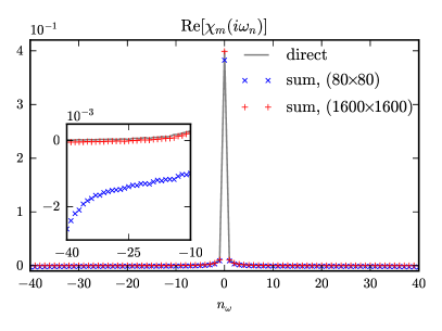
Figure 7: Local susceptibilities $\chi_{\mathrm{loc}}(i\omega_{n})$ in density (top) and magnetic channel (bottom) for the Hubbard model in DMFT at $U=2D$ and $\beta=8/D$. The bosonic Matsubara frequencies are $\omega_{n}=n\frac{2\pi}{\beta}$. We compare the direct calculation via Eq. (22) (solid line) to that using the summation Eq. (41) over Fermionic Matsubara frequencies without vertex asymptotics in a small box (x) to that using vertex asymptotics and hence a large box (+). Inset: zoom in showing the box-effect and noise reduction.

V.2 Multi-orbital test case: SrVO₃

Since the derivations in the previous sections were done without restriction to one-band models or density-density interaction, it is possible to apply the procedure described above to a more general case. As a suitable material, we chose SrVO₃, which has a long tradition for benchmarking realistic material calculations using DMFT.Sekiyama et al. (2004); Ishida et al. (2006); Lee et al. (2012); Taranto et al. (2013); Sakuma et al. (2013) Its band structure can be calculated by wien2k,Schwarz and Blaha (2003) using the generalized gradient approximation. Subsequently, $t_{2g}$ bands, which cross the Fermi level, are projected onto maximally localized Wannier functions by wien2wannier.Kuneš et al. (2010) For these strongly correlated $t_{2g}$ bands we consider a SU(2) symmetric Slater-Kanamori interaction that is parameterized by an intra-orbital Hubbard $U$, an inter-orbital $U^{\prime}$ and Hund’s coupling $J$. Calculations in constrained local density approximation yield values of $U=5$eV, $J=0.75$eV and $U^{\prime}=U-2J=3.5$eV.Sekiyama et al. (2004); Nekrasov et al. (2006)
The following DMFT calculation, as well as the calculation of the one-, two- and three-frequency two-particle Green’s functions, was done by w2dynamics at an inverse temperature of $\beta=10\mathrm{eV}^{-1}$.
Since we treat SrVO₃ as a three-orbital system, the two-particle objects have in general have $(2\cdot 3)^{4}=1296$ spin-orbital components, of which due to the structure of the interaction, however, only 126 are non-vanishing. If we use instead of all spin-components the density and magnetic channels, which is possible for SU(2) symmetry, the number of non-vanishing components is reduced to 21 per channel. Furthermore the local vertex functions exhibit orbital symmetry that reduces the number of distinct components to 4 per channel in our case of degenerate orbitals.
In Fig. 8 a slice of the vertex with four equal band indices is shown in the density and magnetic channel: $F_{d/m,1111}^{\nu\nu^{\prime}\omega_{15}}$. As before, in the left column we show the vertex, as calculated by amputation of external legs from the susceptibility with full frequency dependence. This is the way how the multi-orbital vertex was determined previously in AbinitioD$\Gamma$A calculations.Galler et al. (2017) In the right column, we present the same vertex, but now the data at asymptotic values of the frequency, given by Eq. (40) with $l=15$, are replaced by the asymptotic vertex. Our approach reduces the noise considerably and makes multi-orbital vertex calculations much more feasible.

Figure 8: (Color online) Matrix element of the full vertex $F_{d,1111}^{\nu\nu^{\prime}\omega_{15}}$ (upper row) and $F_{m,1111}^{\nu\nu^{\prime}\omega_{15}}$ (lower row) for four times at the same $t_{2g}$ orbital. Left column: $F$ extracted from an improved-estimator CT-QMC measurement with full frequency dependence. Right column: $F$, combined with asymptotics according to Eq. (40) with $l=15$. To remove the constant background, $F_{d}$ was shifted by $U_{d}=U$ and $F_{m}$ by $U_{m}=-U$.

In order to show how the fully frequency-dependent vertex $F$ approaches its asymptotic form, we show in Fig. 9 three slices of the difference $F-F_{\mathrm{asympt}}$. Again a strong decay can be noticed, albeit slower than in the Hubbard model studied above. Furthermore the diagonal defined by $\nu_{ph}=\nu_{\mkern 1.5mu\overline{\mkern-1.5muph\mkern-1.5mu}\mkern 1.5mu}$ is considerably more pronounced, a behavior that is to be expected, however, by atomic limit calculations.

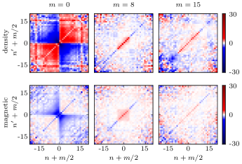
Figure 9: (Color online) Difference of $F_{d,1111}^{\nu\nu^{\prime}\omega_{15}}$ (top) and $F_{m,1111}^{\nu\nu^{\prime}\omega_{15}}$ (bottom) to their respective purely asymptotic version. for different bosonic frequencies $\omega_{m}=\frac{2\pi}{\beta}m$.

A sample application of the asymptotics is again the calculation of frequency-summed susceptibilities. In order to demonstrate the ability of our method to treat pair hopping and spin flip contributions, introduced by the SU(2) symmetric Kanamori interaction, we show the components $\chi^{d/m,\omega}_{1122}$ in Fig. 10. Two important observations can be made in these plots: First, the noise can be largely reduced in the high-frequency region, and second, large deviations at $\omega=0$ can be eliminated.

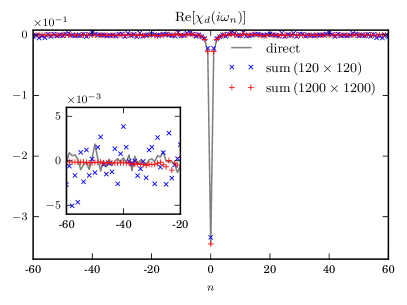
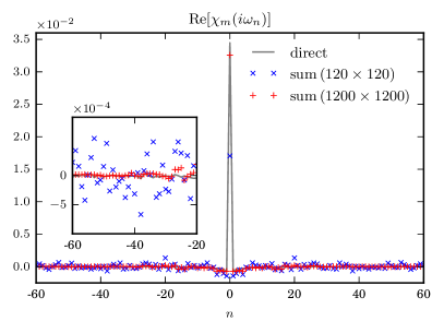
Figure 10: (Color online) Local susceptibility $\chi^{\mathrm{loc}}_{d/m,1122}$ of SrVO₃ between two different $t_{2g}$ orbitals in density (top) and magnetic channel (bottom). Inset: zoom in.

VI Conclusion

In this work we establish the link between reduced frequency (equal-time) two-particle Green’s functions and the asymptotics of the full vertex function $F$ for the multi-orbital AIM. The former ones are, in principle, accessible by employing impurity solvers such as CT-QMC. We make use of a worm algorithm in the hybridization expansion to measure these equal-time Green’s functions in CT-QMC for multiple orbitals and general local interactions. From these Green’s functions in turn, we calculate the Kernel-1 and Kernel-2 functions for the vertex asymptotics. This requires contractions with the bare interaction and a careful treatment of the disconnected parts. We benchmark the vertex asymptotics for the single-orbital Hubbard model in DMFT, by comparing our numerical CT-QMC data to ED results. As a second application, we calculate the vertex asymptotics for SrVO₃ using three $t_{2g}$ orbitals for the low energy degrees of freedom. In both cases, we demonstrate that using the asymptotics yields a much better vertex with less noise and for an arbitrary large frequency box. The latter allows us to avoid the errors associated a finite frequency box when calculating physical susceptibilities.

Our method allows us to assemble multi-orbital vertices in CT-QMC for arbitrary frequency boxes, at a much reduced computational time and storage. A second advantage is that we overcome the problem of noisy QMC vertices at larger frequencies. Our paper is hence a crucial step for making the (multi-orbital) vertex available both for calculating general DMFT susceptibilities and for diagrammatic extensions to DMFT.

Appendix A Frequency mappings

Two-particle functions have four fermionic frequency arguments $\nu_{1}\ldots\nu_{4}$. Due to energy conservation, one of the arguments is redundant and we use one bosonic and two fermionic frequency arguments instead. Since the mapping between those two sets of frequencies is ambiguous, there exist different possibilities that can be associated to the scattering channels. They are called particle-particle notation ($pp$), particle-hole notation ($ph$) and transverse particle-hole notation ($\mkern 1.5mu\overline{\mkern-1.5muph\mkern-1.5mu}\mkern 1.5mu$).
We thus introduce, in addition to $\nu_{1}\ldots\nu_{4}$, the particle-particle frequencies $\nu_{pp}$, $\nu^{\prime}_{pp}$ and $\omega_{pp}$; the particle-hole frequencies $\nu_{ph}$, $\nu^{\prime}_{ph}$ and $\omega_{ph}$; and the transverse particle-hole frequencies $\nu_{\mkern 1.5mu\overline{\mkern-1.5muph\mkern-1.5mu}\mkern 1.5mu}$, $\nu^{\prime}_{\mkern 1.5mu\overline{\mkern-1.5muph\mkern-1.5mu}\mkern 1.5mu}$ and $\omega_{\mkern 1.5mu\overline{\mkern-1.5muph\mkern-1.5mu}\mkern 1.5mu}$. They are defined in the following way:

$$\nu_{1} =\nu_{pp} = \nu_{ph} = \nu_{\mkern 1.5mu\overline{\mkern-1.5muph\mkern-1.5mu}\mkern 1.5mu}$$ (42)

$$\nu_{2} =\omega_{pp}-\nu^{\prime}_{pp} = \nu_{ph}-\omega_{ph} = \nu^{\prime}_{\mkern 1.5mu\overline{\mkern-1.5muph\mkern-1.5mu}\mkern 1.5mu}$$ (43)

$$\nu_{3} =\omega_{pp}-\nu_{pp} = \nu^{\prime}_{ph}-\omega_{ph} = \nu^{\prime}_{\mkern 1.5mu\overline{\mkern-1.5muph\mkern-1.5mu}\mkern 1.5mu}-\omega_{\mkern 1.5mu\overline{\mkern-1.5muph\mkern-1.5mu}\mkern 1.5mu}$$ (44)

$$\nu_{4} =\nu^{\prime}_{pp} = \nu^{\prime}_{ph} = \nu_{\mkern 1.5mu\overline{\mkern-1.5muph\mkern-1.5mu}\mkern 1.5mu}-\omega_{\mkern 1.5mu\overline{\mkern-1.5muph\mkern-1.5mu}\mkern 1.5mu}$$ (45)

It is convenient to express all frequencies in all possible combinations:

$$\nu_{pp} =\nu_{ph}=\nu_{\mkern 1.5mu\overline{\mkern-1.5muph\mkern-1.5mu}\mkern 1.5mu}$$ (46)

$$\nu^{\prime}_{pp} =\nu^{\prime}_{ph}=\nu_{\mkern 1.5mu\overline{\mkern-1.5muph\mkern-1.5mu}\mkern 1.5mu}-\omega_{\mkern 1.5mu\overline{\mkern-1.5muph\mkern-1.5mu}\mkern 1.5mu}$$ (47)

$$\omega_{pp} =\nu_{ph}+\nu^{\prime}_{ph}-\omega_{ph}=\nu_{\mkern 1.5mu\overline{\mkern-1.5muph\mkern-1.5mu}\mkern 1.5mu}+\nu^{\prime}_{\mkern 1.5mu\overline{\mkern-1.5muph\mkern-1.5mu}\mkern 1.5mu}-\omega_{\mkern 1.5mu\overline{\mkern-1.5muph\mkern-1.5mu}\mkern 1.5mu}$$ (48)

$$\omega_{ph} =\nu_{pp}+\nu^{\prime}_{pp}-\omega_{pp}=\nu_{\mkern 1.5mu\overline{\mkern-1.5muph\mkern-1.5mu}\mkern 1.5mu}-\nu^{\prime}_{\mkern 1.5mu\overline{\mkern-1.5muph\mkern-1.5mu}\mkern 1.5mu}$$ (49)

$$\nu^{\prime}_{\mkern 1.5mu\overline{\mkern-1.5muph\mkern-1.5mu}\mkern 1.5mu} =\nu_{ph}-\omega_{ph}=\omega_{pp}-\nu^{\prime}_{pp}$$ (50)

$$\omega_{\mkern 1.5mu\overline{\mkern-1.5muph\mkern-1.5mu}\mkern 1.5mu} =\nu_{ph}-\nu^{\prime}_{ph}=\nu_{pp}-\nu^{\prime}_{pp}$$ (51)

Appendix B Calculations in the atomic limit

We also validated our approach in the atomic limit, which is obtained by setting the hybridization to $V=0$ in the Anderson impurity model, i. e.

$$H=-\mu(n_{\uparrow}+n_{\downarrow})+Un_{\uparrow}n_{\downarrow}.$$ (52)

In this case, expectation values in the grand canonical ensemble with a Boltzmann weight $\rho\sim\mathrm{exp}[-\beta H]$ and a chemical potential $\mu$ can be calculated analytically in the Lehmann basis $\left\{\left|0\right>,\left|\uparrow\right>,\left|\downarrow\right>,\left|\uparrow\downarrow\right>\right\}$. At half filling, $\mu=U/2$ and thus, $\rho=\mathrm{diag}[1,e^{\beta\mu},e^{\beta\mu},1]/(2+2e^{\beta\mu})$. Expectation values can be calculated as $\langle\mathcal{O}\rangle=\mathrm{Tr}[\mathcal{O}\rho]$. In this way, one can calculate the full two-particle Green’s function and, subsequently, the full vertex $F$.Rohringer et al. (2012); Rohringer (2013) In Ref. Wentzell et al., the Kernel functions were calculated by taking high-frequency limits (see Eq. (15) in Ref. Wentzell et al., ).

On the other hand, we can obtain the vertex asymptotics via the procedure derived in Section III of the present paper. To this end, we first need to calculate the equal-time two-particle Green’s functions, which are given in Table 1 and Table 2, using the Fermi function $f(\varepsilon)\equiv 1/(1+e^{\beta\varepsilon})$ as an abbreviation.

$G_{\sigma\sigma^{\prime}}^{\ell,\omega}$	$pp$	$ph$
$\uparrow\uparrow$	$0$	$\frac{\beta}{2}\delta_{\omega 0}$
$\uparrow\downarrow$	$\frac{\beta}{2}f\left(\frac{U}{2}\right)\delta_{\omega 0}$	$\frac{\beta}{2}f\left(\frac{U}{2}\right)\delta_{\omega 0}$
$\mkern 1.5mu\overline{\mkern-1.5mu\uparrow\downarrow\mkern-1.5mu}\mkern 1.5mu$	$-\frac{\beta}{2}f\left(\frac{U}{2}\right)\delta_{\omega 0}$	$\frac{\beta}{2}f\left(-\frac{U}{2}\right)\delta_{\omega 0}$

Table 1: Two-legged two-particle Green’s functions in the atomic limit, i.e. Eq. (14) and Eq. (15), in particle-particle and particle-hole channel, respectively. Frequencies are given in the channel-specific notations, see Appendix A.

$G_{\sigma\sigma^{\prime}}^{pp,\nu\omega}$
$\uparrow\uparrow$	$0$
$\uparrow\downarrow$	$\frac{\nu(\nu-\omega)-\frac{U^{2}}{4}}{\left(\nu^{2}+\frac{U^{2}}{4}\right)\left((\nu-\omega)^{2}+\frac{U^{2}}{4}\right)}-\delta_{\omega 0}\frac{\beta\frac{U}{2}f\left(\frac{U}{2}\right)}{\nu^{2}+\frac{U^{2}}{4}}$
$\mkern 1.5mu\overline{\mkern-1.5mu\uparrow\downarrow\mkern-1.5mu}\mkern 1.5mu$	$-\frac{\nu(\nu-\omega)-\frac{U^{2}}{4}}{\left(\nu^{2}+\frac{U^{2}}{4}\right)\left((\nu-\omega)^{2}+\frac{U^{2}}{4}\right)}+\delta_{\omega 0}\frac{\beta\frac{U}{2}f\left(\frac{U}{2}\right)}{\nu^{2}+\frac{U^{2}}{4}}$
$G_{\sigma\sigma^{\prime}}^{ph,\nu\omega}$
$\uparrow\uparrow$	$\frac{\nu(\nu-\omega)-\frac{U^{2}}{4}}{\left(\nu^{2}+\frac{U^{2}}{4}\right)\left((\nu-\omega)^{2}+\frac{U^{2}}{4}\right)}+\delta_{\omega 0}\frac{\beta}{2}\frac{\frac{U}{2}\mathrm{tanh}\frac{\beta U}{4}+i\nu}{\nu^{2}+\frac{U^{2}}{4}}$
$\uparrow\downarrow$	$\delta_{\omega 0}\frac{\beta}{2}\frac{-\frac{U}{2}+i\nu}{\nu^{2}+\frac{U^{2}}{4}}$
$\mkern 1.5mu\overline{\mkern-1.5mu\uparrow\downarrow\mkern-1.5mu}\mkern 1.5mu$	$\frac{\nu(\nu-\omega)-\frac{U^{2}}{4}}{\left(\nu^{2}+\frac{U^{2}}{4}\right)\left((\nu-\omega)^{2}+\frac{U^{2}}{4}\right)}+\delta_{\omega 0}\frac{\beta\frac{U}{2}f\left(-\frac{U}{2}\right)}{\nu^{2}+\frac{U^{2}}{4}}$

Table 2: Three-time two-particle Green’s functions in the atomic limit, i.e. Eq. (20) and Eq. (21), in particle-particle and particle-hole channel. Frequencies are given in the channel-specific notations, see Appendix A

In the following we will calculate only the ${\uparrow\downarrow}$-components of the Kernel functions in the $ph$-channel explicitly, but all components are given in Table 3 and Table 4. First, the single-frequency susceptibility is recovered from the respective Green’s function by subtracting the constant density term $\beta\delta_{\omega 0}/4$:

$$\chi^{ph,\omega}_{\uparrow\downarrow}=G^{ph,\omega}_{\uparrow\downarrow}-\frac{\beta\delta_{\omega 0}}{4}=-\frac{1}{4}\beta\delta_{\omega 0}\left[f\left(-\frac{U}{2}\right)-f\left(\frac{U}{2}\right)\right].$$ (53)

Since the single-orbital U-matrix has only four non-vanishing components $U_{\uparrow\downarrow\uparrow\downarrow}=U_{\downarrow\uparrow\downarrow\uparrow}=U$ and $U_{\uparrow\downarrow\downarrow\uparrow}=U_{\downarrow\uparrow\uparrow\downarrow}=-U$, the Kernel function $K^{(1),ph,\omega}_{\uparrow\downarrow}$ is directly related to $\chi^{ph,\omega}_{\downarrow\uparrow}$ by (26):

$$K^{(1),ph,\omega}_{\uparrow\downarrow}=-U^{2}\chi^{ph,\omega}_{\downarrow\uparrow}$$ (54)

Table 3 lists the other Kernel-I functions.

In order to extract $K^{(2),ph,\nu\omega}_{\uparrow\downarrow}$ from equal-time two-particle Green’s functions, it is of advantage to rewrite the latter, emphasizing their connection to one-particle Green’s functions. Since the U-matrix contraction relates $K^{(2),ph,\nu\omega}_{\uparrow\downarrow}$ to $G^{ph,\nu\omega}_{\uparrow\uparrow}$ only, we print the ${\uparrow\uparrow}$-component:

$$G^{ph,\nu\omega}_{\uparrow\uparrow}=-\frac{1}{2}\beta\delta_{\omega 0}G^{\nu}-G^{\nu}G^{\nu-\omega}+\\ +\underbrace{\left[\frac{U^{2}}{4\nu(\nu-\omega)}-\frac{K^{(1),ph,\omega}_{\uparrow\downarrow}}{U}\left(1+\frac{U^{2}}{4\nu^{2}}\right)\right]}_{\equiv-L^{ph,\nu\omega}_{\uparrow\uparrow}}G^{\nu}G^{\nu-\omega}.$$ (55)

From this, the kernel part $L^{ph,\nu\omega}_{\uparrow\uparrow}$ is obtained by subtracting the disconnected parts (first line of the right-hand side) and amputating the legs $G^{\nu}G^{\nu-\omega}$. In a final step, the Kernel function $K^{(2),ph,\nu\omega}_{{\uparrow\downarrow}}$ follows as

$$K^{(2),ph,\nu\omega}_{{\uparrow\downarrow}}=UL^{ph,\nu\omega}_{\uparrow\uparrow}-K^{(1),ph,\omega}_{{\uparrow\downarrow}}\\ =\frac{U^{2}}{4\nu(\nu-\omega)}(K^{(1),pp,\omega}_{\uparrow\downarrow}-U).$$ (56)

Table 4 lists the other Kernel-2 functions. Apart from the different frequency conventions, our formulas agree with the results reported previously.Wentzell et al.

Using (54), (56) and the crossing relation (16) to calculate the Kernel functions in the $\mkern 1.5mu\overline{\mkern-1.5muph\mkern-1.5mu}\mkern 1.5mu$-channel, we can now compile the full asymptotic vertex from its $ph$-, $\mkern 1.5mu\overline{\mkern-1.5muph\mkern-1.5mu}\mkern 1.5mu$- and $pp$-contributions. This is illustrated in Fig. 11, where each of the pictures corresponds to one line of the right-hand side of Eq. (34).

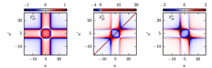
Figure 11: The $ph$-, $\mkern 1.5mu\overline{\mkern-1.5muph\mkern-1.5mu}\mkern 1.5mu$- and $pp$-parts of the asymptotic vertex $F_{\uparrow\downarrow}^{\mathrm{asympt},\nu\nu^{\prime}\omega_{10}}-U$ in $ph$-notation at $U=2$ and $\beta=8$.

Having at our disposal the asymptotic vertex, it is now possible to calculate how it deviates from the complete vertex, similarly as it was done with the numerical data of the Hubbard model and SrVO₃ above. Since the explicit analytical form of the asymptotic vertex is rather lengthy, we print only the difference $R=F-F^{\mathrm{asympt}}$, which is, however, of much greater interest:

$$R_{\uparrow\downarrow}^{\nu_{1}\nu_{2}\nu_{3}\nu_{4}}=\frac{1}{\nu_{1}\nu_{2}\nu_{3}\nu_{4}}\left[-\frac{3U^{5}}{16}+\frac{\beta U^{6}}{64}\left(f\left(-\frac{U}{2}\right)-f\left(\frac{U}{2}\right)\right)\delta_{\nu_{1}\nu_{2}}\\ +\frac{\beta U^{6}}{32}\left(-\frac{U}{2}\right)\delta_{\nu_{1}\nu_{4}}-\frac{\beta U^{6}}{32}2f\left(\frac{U}{2}\right)\delta_{-\nu_{1}\nu_{3}}\right].$$ (57)

Furthermore, we have

$$R_{\uparrow\uparrow}^{\nu_{1}\nu_{2}\nu_{3}\nu_{4}}=\frac{\beta U^{6}}{64}\frac{\delta_{\nu_{1}\nu_{4}}-\delta_{\nu_{1},-\nu_{3}}}{\nu_{1}\nu_{2}\nu_{3}\nu_{4}}$$ (58)

and

$$R_{\mkern 1.5mu\overline{\mkern-1.5mu\uparrow\downarrow\mkern-1.5mu}\mkern 1.5mu}^{\nu_{1}\nu_{2}\nu_{3}\nu_{4}}=-R_{\uparrow\downarrow}^{\nu_{1}\nu_{4}\nu_{3}\nu_{2}}$$ (59)

for the other spin-components. Slices of the purely asymptotic vertex $F^{\mathrm{asympt}}_{\uparrow\downarrow}$ and the difference to the full vertex $R_{\uparrow\downarrow}$ are shown in Fig. 12. We observe that indeed the differences of the full and asymptotic vertices go to zero with $1/(\nu_{1}\nu_{2}\nu_{3}\nu_{4})$ for all components, meeting our initial requirement. Together with the delta-functions, Eq. (57) also motivates the asymptotic replacement condition Eq. (40).

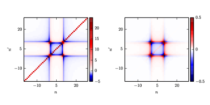
Figure 12: $F_{\uparrow\downarrow}^{\mathrm{asympt,\nu\nu^{\prime}\omega_{10}}}$ (left) and $R_{\uparrow\downarrow}^{\nu\nu^{\prime}\omega_{10}}$ (right) in $ph$-notation at $U=2$ and $\beta=8$.

$K^{(1),\ell,\omega}$	$pp$	$ph$
$\uparrow\uparrow$	$0$	$-\frac{\beta U^{2}}{4}\delta_{\omega 0}$
$\uparrow\downarrow$	$-\frac{\beta U^{2}}{2}f\left(\frac{U}{2}\right)\delta_{\omega 0}$	$\frac{\beta U^{2}}{4}\left[f\left(-\frac{U}{2}\right)-f\left(\frac{U}{2}\right)\right]\delta_{\omega 0}$
$\mkern 1.5mu\overline{\mkern-1.5mu\uparrow\downarrow\mkern-1.5mu}\mkern 1.5mu$	$\frac{\beta U^{2}}{2}f\left(\frac{U}{2}\right)\delta_{\omega 0}$	$-\frac{\beta U^{2}}{2}f\left(-\frac{U}{2}\right)\delta_{\omega 0}$

Table 3: Kernel functions $K^{(1)}$ in particle-particle and particle-hole channel. Frequencies are given in the channel-specific notations, see Appendix A.

$K^{(2),\ell,\nu\omega}$	$pp$	$ph$
$\uparrow\uparrow$	$0$	$K^{(1),ph,\omega}_{\uparrow\uparrow}\frac{U^{2}}{4\nu^{2}}$
$\uparrow\downarrow$	$\frac{U^{2}}{4\nu(\nu-\omega)}(K^{(1),pp,\omega}_{\uparrow\downarrow}-U)$	$\frac{U^{2}}{4\nu(\nu-\omega)}(K^{(1),ph,\omega}_{\uparrow\downarrow}-U)$
$\mkern 1.5mu\overline{\mkern-1.5mu\uparrow\downarrow\mkern-1.5mu}\mkern 1.5mu$	$-\frac{U^{2}}{4\nu(\nu-\omega)}(K^{(1),pp,\omega}_{\uparrow\downarrow}-U)$	$\frac{U^{2}}{4\nu(\nu-\omega)}(K^{(1),ph,\omega}_{\mkern 1.5mu\overline{\mkern-1.5mu\uparrow\downarrow\mkern-1.5mu}\mkern 1.5mu}+U)$

Table 4: Kernel functions $K^{(2)}$ in particle-particle and particle-hole channel. Frequencies are given in the channel-specific notations, see Appendix A.

References

- Mott (1968) N. F. Mott, Rev. Mod. Phys. 40, 677 (1968), URL http://link.aps.org/doi/10.1103/RevModPhys.40.677.
- Georges et al. (1996) A. Georges, G. Kotliar, W. Krauth, and M. J. Rozenberg, Rev. Mod. Phys. 68, 13 (1996), URL http://link.aps.org/doi/10.1103/RevModPhys.68.13.
- Löhneysen et al. (1994) H. v. Löhneysen, T. Pietrus, G. Portisch, H. G. Schlager, A. Schröder, M. Sieck, and T. Trappmann, Phys. Rev. Lett. 72, 3262 (1994), URL http://link.aps.org/doi/10.1103/PhysRevLett.72.3262.
- Rohringer et al. (2011a) G. Rohringer, A. Toschi, A. Katanin, and K. Held, Phys. Rev. Lett. 107, 256402 (2011a), URL http://link.aps.org/doi/10.1103/PhysRevLett.107.256402.
- Schroder et al. (2000) A. Schroder, G. Aeppli, R. Coldea, M. Adams, O. Stockert, H. v. Lohneysen, E. Bucher, R. Ramazashvili, and P. Coleman, Nature 407, 351 (2000), URL http://dx.doi.org/10.1038/35030039.
- Schäfer et al. (2016a) T. Schäfer, A. Katanin, K. Held, and A. Toschi (2016a), eprint 1605.06355, URL http://arxiv.org/abs/1605.06355.
- LeBlanc et al. (2015) J. P. F. LeBlanc, A. E. Antipov, F. Becca, I. W. Bulik, G. K.-L. Chan, C.-M. Chung, Y. Deng, M. Ferrero, T. M. Henderson, C. A. Jiménez-Hoyos, et al. (Simons Collaboration on the Many-Electron Problem), Phys. Rev. X 5, 041041 (2015), URL http://link.aps.org/doi/10.1103/PhysRevX.5.041041.
- Hubbard (1963) J. Hubbard, Proceedings of the Royal Society of London. Series A. Mathematical and Physical Sciences 276, 238 (1963), URL http://rspa.royalsocietypublishing.org/content/276/1365/238.abstract.
- Metzner and Vollhardt (1989) W. Metzner and D. Vollhardt, Phys. Rev. Lett. 62, 324 (1989), URL http://link.aps.org/doi/10.1103/PhysRevLett.62.324.
- Georges and Kotliar (1992) A. Georges and G. Kotliar, Phys. Rev. B 45, 6479 (1992), URL http://link.aps.org/doi/10.1103/PhysRevB.45.6479.
- Kotliar and Vollhardt (2004) G. Kotliar and D. Vollhardt, Physics Today 57, 53 (2004), URL http://dx.doi.org/10.1063/1.1712502.
- Held (2007) K. Held, Advances in Physics 56, 829 (2007), URL http://dx.doi.org/10.1080/00018730701619647.
- Anderson (1961) P. W. Anderson, Phys. Rev. 124, 41 (1961), URL http://link.aps.org/doi/10.1103/PhysRev.124.41.
- Hirsch and Fye (1986) J. E. Hirsch and R. M. Fye, Phys. Rev. Lett. 56, 2521 (1986), URL http://link.aps.org/doi/10.1103/PhysRevLett.56.2521.
- Sakai et al. (2006) S. Sakai, R. Arita, K. Held, and H. Aoki, Phys. Rev. B 74, 155102 (2006), URL http://link.aps.org/doi/10.1103/PhysRevB.74.155102.
- Bulla et al. (2008) R. Bulla, T. A. Costi, and T. Pruschke, Rev. Mod. Phys. 80, 395 (2008), URL http://link.aps.org/doi/10.1103/RevModPhys.80.395.
- Karski et al. (2008) M. Karski, C. Raas, and G. S. Uhrig, Phys. Rev. B 77, 075116 (2008), URL http://link.aps.org/doi/10.1103/PhysRevB.77.075116.
- Ganahl et al. (2014) M. Ganahl, P. Thunström, F. Verstraete, K. Held, and H. G. Evertz, Phys. Rev. B 90, 045144 (2014), URL http://link.aps.org/doi/10.1103/PhysRevB.90.045144.
- Caffarel and Krauth (1994) M. Caffarel and W. Krauth, Phys. Rev. Lett. 72, 1545 (1994), URL http://link.aps.org/doi/10.1103/PhysRevLett.72.1545.
- Zgid et al. (2012) D. Zgid, E. Gull, and G. K.-L. Chan, Phys. Rev. B 86, 165128 (2012), URL http://link.aps.org/doi/10.1103/PhysRevB.86.165128.
- Rubtsov and Lichtenstein (2004) A. Rubtsov and A. Lichtenstein, Journal of Experimental and Theoretical Physics Letters 80, 61 (2004), URL http://dx.doi.org/10.1134/1.1800216.
- Werner et al. (2006) P. Werner, A. Comanac, L. de’ Medici, M. Troyer, and A. J. Millis, Phys. Rev. Lett. 97, 076405 (2006), URL http://link.aps.org/doi/10.1103/PhysRevLett.97.076405.
- Werner and Millis (2006) P. Werner and A. J. Millis, Phys. Rev. B 74, 155107 (2006), URL http://link.aps.org/doi/10.1103/PhysRevB.74.155107.
- Gull et al. (2008) E. Gull, P. Werner, O. Parcollet, and M. Troyer, EPL (Europhysics Letters) 82, 57003 (2008), URL http://stacks.iop.org/0295-5075/82/i=5/a=57003.
- Gull et al. (2011) E. Gull, A. J. Millis, A. I. Lichtenstein, A. N. Rubtsov, M. Troyer, and P. Werner, Reviews of Modern Physics 83, 349 (2011), URL http://dx.doi.org/10.1103/RevModPhys.83.349.
- Toschi et al. (2007) A. Toschi, A. A. Katanin, and K. Held, Phys. Rev. B 75, 045118 (2007), URL http://link.aps.org/doi/10.1103/PhysRevB.75.045118.
- Rubtsov et al. (2008) A. N. Rubtsov, M. I. Katsnelson, and A. I. Lichtenstein, Phys. Rev. B 77, 033101 (2008), URL http://link.aps.org/doi/10.1103/PhysRevB.77.033101.
- Rohringer et al. (2013) G. Rohringer, A. Toschi, H. Hafermann, K. Held, V. I. Anisimov, and A. A. Katanin, Phys. Rev. B 88, 115112 (2013), URL http://link.aps.org/doi/10.1103/PhysRevB.88.115112.
- Taranto et al. (2014) C. Taranto, S. Andergassen, J. Bauer, K. Held, A. Katanin, W. Metzner, G. Rohringer, and A. Toschi, Phys. Rev. Lett. 112, 196402 (2014), URL http://link.aps.org/doi/10.1103/PhysRevLett.112.196402.
- Ayral and Parcollet (2016) T. Ayral and O. Parcollet, Phys. Rev. B 94, 075159 (2016), URL http://link.aps.org/doi/10.1103/PhysRevB.94.075159.
- Rohringer et al. (2012) G. Rohringer, A. Valli, and A. Toschi, Phys. Rev. B 86, 125114 (2012), URL http://link.aps.org/doi/10.1103/PhysRevB.86.125114.
- Galler et al. (2017) A. Galler, P. Thunström, P. Gunacker, J. M. Tomczak, and K. Held, Phys. Rev. B 95, 115107 (2017), URL http://link.aps.org/doi/10.1103/PhysRevB.95.115107.
- Kuneš (2011) J. Kuneš, Phys. Rev. B 83, 085102 (2011), URL http://link.aps.org/doi/10.1103/PhysRevB.83.085102.
- Li et al. (2016) G. Li, N. Wentzell, P. Pudleiner, P. Thunström, and K. Held, Phys. Rev. B 93, 165103 (2016), URL http://link.aps.org/doi/10.1103/PhysRevB.93.165103.
- (35) N. Wentzell, G. Li, A. Tagliavini, C. Taranto, G. Rohringer, K. Held, A. Toschi, and S. Andergassen, eprint 1610.06520, URL http://arxiv.org/abs/1610.06520.
- Tagliavini et al. (2017) A. Tagliavini, S. Hummel, N. Wentzell, S. Andergassen, A. Toschi, and G. Rohringer (2017), unpublished.
- Schäfer et al. (2013) T. Schäfer, G. Rohringer, O. Gunnarsson, S. Ciuchi, G. Sangiovanni, and A. Toschi, Phys. Rev. Lett. 110, 246405 (2013), URL http://link.aps.org/doi/10.1103/PhysRevLett.110.246405.
- Schäfer et al. (2016b) T. Schäfer, S. Ciuchi, M. Wallerberger, P. Thunström, O. Gunnarsson, G. Sangiovanni, G. Rohringer, and A. Toschi, Phys. Rev. B 94, 235108 (2016b), URL http://link.aps.org/doi/10.1103/PhysRevB.94.235108.
- Gunacker et al. (2015) P. Gunacker, M. Wallerberger, E. Gull, A. Hausoel, G. Sangiovanni, and K. Held, Phys. Rev. B 92, 155102 (2015), URL http://link.aps.org/doi/10.1103/PhysRevB.92.155102.
- Gunacker et al. (2016) P. Gunacker, M. Wallerberger, T. Ribic, A. Hausoel, G. Sangiovanni, and K. Held, Phys. Rev. B 94, 125153 (2016), URL http://link.aps.org/doi/10.1103/PhysRevB.94.125153.
- De Dominicis (1962) C. De Dominicis, J. Math. Phys. 3, 983 (1962), URL http://jmp.aip.org/resource/1/jmapaq/v3/i5/p983_s1.
- De Dominicis and Martin (1964) C. De Dominicis and P. C. Martin, J. Math. Phys. 5, 14 (1964), URL http://jmp.aip.org/resource/1/jmapaq/v5/i1/p14_s1.
- Bickers (2004) N. E. Bickers, Theoretical Methods for Strongly Correlated Electrons (Springer-Verlag New York Berlin Heidelbert, 2004), chap. 6, pp. 237–296.
- Shinaoka et al. (2017) H. Shinaoka, E. Gull, and P. Werner, Computer Physics Communications (2017), in press.
- Hafermann (2014) H. Hafermann, Phys. Rev. B 89, 235128 (2014), URL http://link.aps.org/doi/10.1103/PhysRevB.89.235128.
- Rohringer et al. (2011b) G. Rohringer, A. Toschi, A. Katanin, and K. Held, Phys. Rev. Lett. 107, 256402 (2011b), URL http://link.aps.org/doi/10.1103/PhysRevLett.107.256402.
- Parragh et al. (2012) N. Parragh, A. Toschi, K. Held, and G. Sangiovanni, Phys. Rev. B 86, 155158 (2012), URL http://link.aps.org/doi/10.1103/PhysRevB.86.155158.
- Wallerberger (2016) M. Wallerberger, Ph.D. thesis, Vienna University of Technology (2016).
- Sekiyama et al. (2004) A. Sekiyama, H. Fujiwara, S. Imada, S. Suga, H. Eisaki, S. I. Uchida, K. Takegahara, H. Harima, Y. Saitoh, I. A. Nekrasov, et al., Phys. Rev. Lett. 93, 156402 (2004), URL https://link.aps.org/doi/10.1103/PhysRevLett.93.156402.
- Ishida et al. (2006) H. Ishida, D. Wortmann, and A. Liebsch, Phys. Rev. B 73, 245421 (2006), URL https://link.aps.org/doi/10.1103/PhysRevB.73.245421.
- Lee et al. (2012) H. Lee, K. Foyevtsova, J. Ferber, M. Aichhorn, H. O. Jeschke, and R. Valentí, Phys. Rev. B 85, 165103 (2012), URL http://link.aps.org/doi/10.1103/PhysRevB.85.165103.
- Taranto et al. (2013) C. Taranto, M. Kaltak, N. Parragh, G. Sangiovanni, G. Kresse, A. Toschi, and K. Held, Phys. Rev. B 88, 165119 (2013), URL https://link.aps.org/doi/10.1103/PhysRevB.88.165119.
- Sakuma et al. (2013) R. Sakuma, P. Werner, and F. Aryasetiawan, Phys. Rev. B 88, 235110 (2013), URL http://link.aps.org/doi/10.1103/PhysRevB.88.235110.
- Schwarz and Blaha (2003) K. Schwarz and P. Blaha, Computational Materials Science 28, 259 (2003), proceedings of the Symposium on Software Development for Process and Materials Design, URL http://www.sciencedirect.com/science/article/pii/S0927025603001125.
- Kuneš et al. (2010) J. Kuneš, R. Arita, P. Wissgott, A. Toschi, H. Ikeda, and K. Held, Computer Physics Communications 181, 1888 (2010), URL http://www.sciencedirect.com/science/article/pii/S0010465510002948.
- Nekrasov et al. (2006) I. A. Nekrasov, K. Held, G. Keller, D. E. Kondakov, T. Pruschke, M. Kollar, O. K. Andersen, V. I. Anisimov, and D. Vollhardt, Phys. Rev. B 73, 155112 (2006), URL http://link.aps.org/doi/10.1103/PhysRevB.73.155112.
- Hunter (2007) J. D. Hunter, Computing In Science & Engineering 9, 90 (2007).
- Rohringer (2013) G. Rohringer, Ph.D. thesis, Vienna University of Technology (2013).
- Wang et al. (2011) X. Wang, H. T. Dang, and A. J. Millis, Phys. Rev. B 84, 073104 (2011), URL http://link.aps.org/doi/10.1103/PhysRevB.84.073104.