Factoring Exogenous State for Model-Free Monte Carlo

Abstract

Policy analysts wish to visualize a range of policies for large simulator-defined Markov Decision Processes (MDPs). One visualization approach is to invoke the simulator to generate on-policy trajectories and then visualize those trajectories. When the simulator is expensive, this is not practical, and some method is required for generating trajectories for new policies without invoking the simulator. The method of Model-Free Monte Carlo (MFMC) can do this by stitching together state transitions for a new policy based on previously-sampled trajectories from other policies. This “off-policy Monte Carlo simulation” method works well when the state space has low dimension but fails as the dimension grows. This paper describes a method for factoring out some of the state and action variables so that MFMC can work in high-dimensional MDPs. The new method, MFMCi, is evaluated on a very challenging wildfire management MDP.

1 Introduction

As reinforcement learning systems are increasingly deployed in the real-world, methods for justifying their ecological validity becomes increasingly important. For example, consider the problem of wildfire management in which land managers must decide when and where to fight fires on public lands. Our goal is to create an interactive visualization environment in which policy analysts can define various fire management polices and evaluate them through comparative visualizations. The transition dynamics of our fire management MDP are defined by a simulator that takes as input a detailed map of the landscape, an ignition location, a stream of weather conditions, and a fire fighting decision (i.e., suppress the fire vs. allow it to burn), and produces as output the resulting landscape map and associated variables (fire duration, area burned, timber value lost, fire fighting cost, etc.). The simulator also models the year-to-year growth of the trees and accumulation of fuels. Unfortunately, this simulator is extremely expensive. It can take up to 7 hours to simulate a single 100-year trajectory of fire ignitions and resulting landscapes. How can we support interactive policy analysis when the simulator is so expensive?

Our approach is to develop a surrogate model that can substitute for the simulator. We start by designing a small set of “seed policies” and invoking the slow simulator to generate several 100-year trajectories for each policy. This gives us a database of state transitions of the form $(s_{t},a_{t},r_{t},s_{t+1})$, where $s_{t}$ is the state at time $t$, $a_{t}$ is the selected action, $r_{t}$ is the resulting reward, and $s_{t+1}$ is the resulting state. Given a new policy $\pi$ to visualize, we apply the method of Model-Free Monte Carlo (MFMC) developed by Fonteneau et al. (2013) to simulate trajectories for $\pi$ by stitching together state transitions according to a given distance metric $\Delta$. Given a current state $s$ and desired action $a=\pi(s)$, MFMC searches the database to find a tuple $(\tilde{s},\tilde{a},r,s^{\prime})$ that minimizes the distance $\Delta((s,a),(\tilde{s},\tilde{a}))$. It then uses $s^{\prime}$ as the resulting state and $r$ as the corresponding one-step reward. We call this operation “stitching” $(s,a)$ to $(\tilde{s},\tilde{a})$. MFMC is guaranteed to give reasonable simulated trajectories under assumptions about the smoothness of the transition dynamics and reward function and provided that each matched tuple is removed from the database when it is used. Algorithm 1 provides the pseudocode for MFMC generating a single trajectory.

Fonteneau et al. (2010) apply MFMC to estimate the expected cumulative return of a new policy $\pi$ by calling MFMC $n$ times and computing the average cumulative reward of the resulting trajectories. We will refer to this as the MFMC estimate $V_{MFMC}^{\pi}(s_{0})$ of $V^{\pi}(s_{0})$.

Input Parameters: Policy $\pi$, horizon $h$, starting state $s_{0}$, distance metric $\Delta(.,.)$, database $D$;

Returns: $(s,a,r)_{1},...,(s^{\prime},a^{\prime},r^{\prime})_{h}$;

$t\leftarrow\emptyset$;

$s\leftarrow s_{0}$;

while length($t$)$<h$ do

       $a\leftarrow\pi(s)$;

       $\mathcal{H}\leftarrow\underset{(\overset{\sim}{s},\overset{\sim}{a},r,s^{\prime})\in D}{\operatorname*{\arg\!\min}}\Delta((s,a),(\overset{\sim}{s},\overset{\sim}{a}))$;

       $r\leftarrow\mathcal{H}^{r}$;

       append$(t,(s,a,r))$;

       $s\leftarrow\mathcal{H}^{s^{\prime}}$;

       $D\leftarrow D\setminus\mathcal{H}$;

      

end while

return($t$);

Algorithm 1 MFMC for a single trajectory. When generating multiple trajectories for a single trajectory set, you cannot re-use state transitions from $D$ (Fonteneau et al., 2010).

In high-dimensional spaces (i.e., where the states and actions are described by many features), MFMC breaks because of two related problems. First, distances become less informative in high-dimensional spaces. Second, the required number of seed-policy trajectories grows exponentially in the dimensionality of the space. The main technical contribution of this paper is to introduce a modified algorithm, MFMCi, that reduces the dimensionality of the distance matching process by factoring out certain exogenous state variables and removing the features describing the action. In many applications, this can very substantially reduce the dimensionality of the matching process to the point that MFMC is again practical.

This paper is organized as follows. First, we briefly review previous research in surrogate modeling. Second, we introduce our method for factoring out exogenous variables. The method requires a modification to the way that trajectories are generated from the seed policies. With this modification, we prove that MFMCi gives sound results and that it has lower bias and variance than MFMC. Third, we conduct an experimental evaluation of MFMCi on our fire management problem. We show that MFMCi gives good performance for three different classes of policies and that for a fixed database size, it gives much more accurate visualizations.

2 Related Work

Surrogate modeling is the construction of a fast simulator that can substitute for a slow simulator. When designing a surrogate model for our wildfire suppression problem, we can consider several possible approaches.

First, we could write our own simulator for fire spread, timber harvest, weather, and vegetative growth that computes the state transitions more efficiently. For instance, Arca et al. (2013) use a custom-built model running on GPUs to calculate fire risk maps and mitigation strategies. However, developing a new simulator requires additional work to design, implement, and (especially) validate the simulator. This cost can easily overwhelm the resulting time savings.

A second approach would be to learn a parametric surrogate model from data generated by the slow simulator. For instance, Abbeel et al. (2005) learn helicopter dynamics by updating the parameters of a function designed specifically for helicopter flight. Designing a suitable parametric model that can capture weather, vegetation, fire spread, and the effect of fire suppression would require a major modeling effort.

Instead of pursuing these two approaches, we adopted the method of Model-Free Monte Carlo (MFMC). In MFMC, the model is replaced by a database of transitions computed from the slow simulator. MFMC is “model-free” in the sense that it does not learn an explicit model of the transition probabilities. In effect, the database constitutes the transition model (c.f., Dyna; (Sutton, 1990)).

3 Notation

We work with the standard finite horizon undiscounted MDP (Bellman, 1957; Puterman, 1994), denoted by the tuple ${\cal M}=\langle{S,A,P,R,s_{0},h\rangle}$. $S$ is a finite set of states of the world; $A$ is a finite set of possible actions that can be taken in each state; $P:S\times A\times S\mapsto[0,1]$ is the conditional probability of entering state $s^{\prime}$ when action $a$ is executed in state $s$; $R(s,a)$ is the finite reward received after performing action $a$ in state $s$; $s_{0}$ is the starting state; and $\pi:S\mapsto A$ is the policy function that selects which action $a\in A$ to execute in state $s\in S$. We additionally define $D$ as the state transition database.

In this paper, we focus on two queries about a given MDP. First, given a policy $\pi$, we wish to estimate the expected cumulative reward of executing that policy starting in state $s_{0}$: $V^{\pi}(s_{0})=\mathbb{E}[\sum_{t=0}^{h}R(s_{t},\pi(s_{t}))|s_{0},\pi]$. Second, we are interested in visualizing the distribution of the states visited at time $t$: $P(s_{t}|s_{0},\pi)$. In particular, let $v^{1},\ldots,v^{m}$ be functions that compute interesting properties of a state. For example, in our fire domain, $v^{1}(s)$ might compute the total area of old growth Douglas fir and $v^{2}(s)$ might compute the total volume of harvestable wood. Visualizing the distribution of these properties over time gives policy makers insight into how the system will evolve when it is controlled by policy $\pi$.

4 Factoring State to Improve MFMC

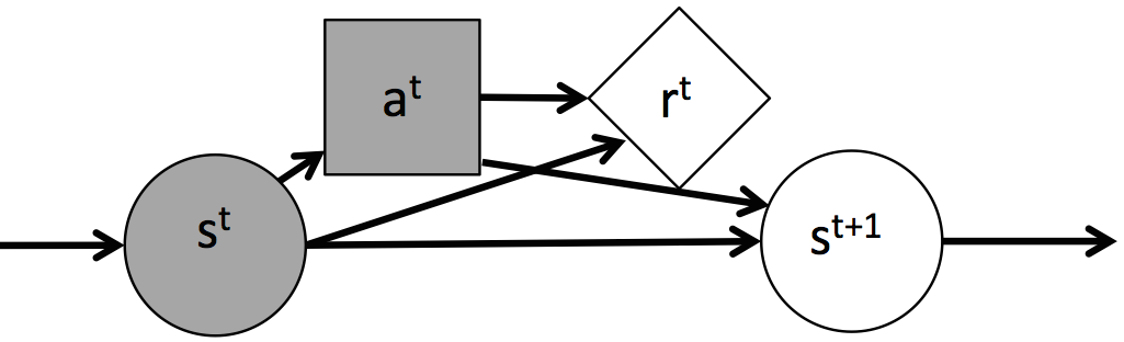
(a) The standard MDP transition.

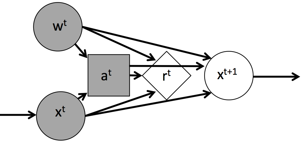
(b) MDP transition with exogenous ($w$) and Markovian variables ($x$).

Figure 1: MDP probabilistic graphical models.

We now describe how we can factor the state variables of an MDP in order to reduce the dimensionality of the MFMC stitching computation. State variables can be divided into Markovian and Time-Independent random variables. A time-independent random variable $x_{t}$ is exchangeable over time $t$ and does not depend on any other random variable (including its own previous values). A (first-order) Markovian random variable $x_{t+1}$ depends on its value $x_{t}$ at the previous time step. In particular, the state variable $s_{t+1}$ depends on $s_{t}$ and the chosen action $a_{t}$. Variables can also be classified as endogenous and exogenous. The variable $x_{t}$ is exogenous if its distribution is independent of $a_{t^{\prime}}$ and $s_{t^{\prime}}\setminus\{x_{t}^{\prime}\}$ for all $t^{\prime}\leq t$. Non-exogenous variables are endogenous. The key insight of this paper is that if a variable is time-independent and exogenous, then it can be removed from the MFMC stitching calculation as follows.

Let us factor the MDP state $s$ into two vectors of random variables: $w$, which contains the time-independent, exogenous state variables and $x$, which contains all of the other state variables (see Figure 1). In our wildfire suppression domain, the state of the trees from one time step to another is Markovian, but our policy decisions also depend on exogenous weather events such as rain, wind, and lightning.

We can formalize this factorization as follows.

Definition 4.1.

A Factored Exogenous MDP is an MDP such that the state $(x,w)$ and next state $(x^{\prime},w^{\prime})$ are related according to

$$Pr(x^{\prime},w^{\prime}|x,w,a)=Pr(w^{\prime})Pr(x^{\prime}|x,w,a).$$ (1)

This factorization allows us to avoid computing similarity in the complete state space $s$. Instead we only need to compute the similarity of the Markov state $x$. Without the factorization, MFMC stitches $(s,a)$ to the $(\tilde{s},\tilde{a})$ in the database $D$ that minimizes a distance metric $\Delta$, where $\Delta$ has the form $\Delta((s,a),(\tilde{s},\tilde{a}))\mapsto\mathbb{R}^{+}$. Our new algorithm, MFMCi, makes its stitching decisions using only the Markov state. It stitches the current state $x$ by finding the tuple $(\tilde{x},\tilde{w},a,r,x^{\prime})$ that minimizes the lower-dimensional distance metric $\Delta_{i}(x,\tilde{x})$. MFMCi then adopts $(\tilde{x},\tilde{w})$ as the current state, computes the policy action $\tilde{a}=\pi(\tilde{x},\tilde{w})$, and then makes a transition to $x^{\prime}$ with reward $r$. The rationale for replacing $x$ by $\tilde{x}$ is the same as in MFMC, namely that it is the nearest state from the database $D$. The rationale for replacing $w$ by $\tilde{w}$ is that both $w$ and $\tilde{w}$ are exchangeable draws from the exogenous time-independent distribution $P(w)$, so they can be swapped without changing the distribution of simulated paths.

Input Parameters: Policy $\pi$, horizon $h$, trajectory count $n$, transition simulator $f_{x}$, reward simulator $f_{r}$, exogenous distribution $P(w)$, stochasticity distribution $P(z)$

Returns: $nh$ transition sets $B$

$D\leftarrow\emptyset$

while $|D|<nh$ do

       $x=f_{x}(\cdot,\cdot,\cdot,\cdot)$ // Draw initial Markov state

       $l=0$

       while $l<h$ do

             $B\leftarrow\emptyset$

             $w\sim P(w)$

             $z\sim P(z)$

             for $a\in A$ do

                   $r\leftarrow f_{r}(x,a,w,z)$

                   $x^{\prime}\leftarrow f_{x}(x,a,w,z)$

                   $B\leftarrow B\cup\{(x,w,a,r,x^{\prime})\}$

                  

             end for

            append($D$,$B$)

             $x\leftarrow B_{\pi(x,w)}^{x^{\prime}}$

             $l\leftarrow l+1$

            

       end while

      

end while

return($D$)

Algorithm 2 Populating $D$ for MFMCi by sampling whole trajectories.

There is one subtlety that can introduce bias into the simulated trajectories. What happens when the action $\tilde{a}=\pi(\tilde{x},\tilde{w})$ is not equal to the action $a$ in the database tuple $(\tilde{x},\tilde{w},a,r,x^{\prime},w^{\prime})$? One approach would be to require that $a=\tilde{a}$ and keep rejecting candidate tuples until we find one that satisfies this constraint. We call this method, “Biased MFMCi”, because doing this introduces a bias. Consider again the graphical model in Figure 1. When we use the value of $a$ to decide whether to accept $\tilde{w}$, this couples $\tilde{w}$ and $\tilde{x}$ so that they are no longer independent.

An alternative to Biased MFMCi is to change how we generate the database $D$ to ensure that for every state $(\tilde{x},\tilde{w})$, there is always a tuple $(\tilde{x},\tilde{w},a,r,x^{\prime},w^{\prime})$ for every possible action $a$. To do this, as we execute a trajectory following policy $\pi$, we simulate the result state $(x^{\prime},w^{\prime})$ and reward $r$ for each possible action $a$ and not just the action $a=\pi(x,w)$ dictated by the policy. We call this method “Debiased MFMCi”. This requires drawing more samples during database construction, but it restores the independence of $\tilde{w}$ from $\tilde{x}$.

4.1 MFMC with independencies (MFMCi)

For purposes of analyzing MFMCi, it is helpful to make the stochasticity of $P(s^{\prime}|s,a)$ explicit. To do this, let $z$ be a time-independent random variable distributed according to $P(z)$. Then we can “implement” the stochastic transition $P(s^{\prime}|s,a)$ in terms of a random draw of $z$ and a state transition function $f_{x}$ as follows. To make a state transition from state $s=(w,x)$ and action $a$, we draw samples of both the exogenous variable $w^{\prime}\sim P(w^{\prime})$ and from $z\sim P(z)$ and then evaluate the function $x^{\prime}=f_{x}(x,w,a,z)$. The result state $s^{\prime}$ is then $(x^{\prime},w^{\prime})$. Similarly, to model stochastic rewards, we can define the function $f_{r}$ such that $r:=f_{r}(x,w,a,z)$. This encapsulates all of the randomness in $P(s^{\prime}|s,a)$ and $R(s,a)$ in the variables $w^{\prime}$ and $z$.

As noted in the previous section, stitching only on $x$ can introduce bias unless we simulate the effect of every action $a$ for every $x\in D$. It is convenient to collect together all of these simulated successor states and rewards into transition sets. Let $B(x,w)$ denote the transition set of tuples $\{(x,w,a,x^{\prime},r)\}$ generated by simulating each action $a$ in state $(x,w)$. Given a transition set $B$, it is useful to define selector notation as follows. Subscripts of $B$ constrain the set of matching tuples and superscripts indicate which variable is extracted from the matching tuples. Hence, $B_{a}^{x^{\prime}}$ denotes the result state $x^{\prime}$ for the tuple in $B$ that matches action $a$. With this notation, Algorithm 2 describes the process of populating the database with transition sets.

Input Parameters: Policy $\pi$, horizon $h$, starting state $x_{0}$, distance metric $\Delta_{i}(\cdot,\cdot)$, database $D$

Returns: $(x_{0},w,a,r)_{1},\ldots,(x^{\prime},w^{\prime},a^{\prime},r^{\prime})_{h}$

$t\leftarrow\emptyset$

$x\leftarrow x_{0}$

while length($t$)$<h$ do

       $\hat{B}\leftarrow\operatorname*{\arg\!\min}_{B\in D}\Delta_{i}(x,B^{x^{\prime}})$

       $\hat{w}\leftarrow\hat{B}^{w}$

       $a\leftarrow\pi(x,\hat{w})$

       $r\leftarrow\hat{B}^{r}_{a}$

       append$(t,(x,w,a,r))$

       $D\leftarrow D\setminus\hat{B}$

       $x\leftarrow B^{x^{\prime}}_{a}$

      

end while

return($t$)

Algorithm 3 MFMCi

Algorithm 3 gives the pseudo-code for MFMCi. Note that when generating multiple trajectories with Algorithm 3 for a single policy query, the transition sets are drawn without replacement between trajectories. To estimate the cumulative return of policy $\pi$, we call MFMCi $n$ times and compute the mean of the cumulative rewards of the resulting trajectories. We refer to this as the MFMCi estimate $V_{MFMCi}^{\pi}(s_{0})$ of $V^{\pi}(s_{0})$.

4.2 Bias and Variance Bound on $V_{MFMCi}^{\pi}(s_{0})$

Fonteneau et al. (2013; 2014; 2010) derived bias and variance bounds on the MFMC value estimate $V_{MFMC}^{\pi}(s_{0})$. Here we rework this derivation to provide analogous bounds for $V_{MFMCi}^{\pi}(s_{0})$. The Fonteneau et al. bounds depend on assuming Lipschitz smoothness of the functions $f_{s}$, $f_{r}$ and the policy $\pi$. To do this, they require that the action space be continuous in a metric space $A$. We will impose the same requirement for purposes of analysis. Let $L_{f}$, $L_{R}$, and $L_{\pi}$ be Lipschitz constants for the chosen norms $\|\cdot\|_{S}$ and $\|\cdot\|_{A}$ over the $S$ and $A$ spaces, as follows:

$$\|f_{s}(s,a,z)-f_{s}(s^{\prime},a^{\prime},z)\|_{S}~{}\leq~{}L_{f}(\|s-s^{\prime}\|_{S}+\|a-a^{\prime}\|_{A})\\$$ (2)

$$|f_{r}(s,a,z)-f_{r}(s^{\prime},a^{\prime},z)|~{}\leq~{}L_{R}(\|s-s^{\prime}\|_{S}+\|a-a^{\prime}\|_{A})\\$$ (3)

$$\|\pi(s)-\pi(s^{\prime})\|_{A}\leq L_{\pi}(\|s-s^{\prime}\|_{S}).\\$$ (4)

To characterize the database’s coverage of the state-action space, let $\alpha_{k}(D)$ be the maximum distance from any state-action pair $(s,a)$ to its $k$-th nearest neighbor in database $D$. Fonteneau, et al. call this the $k$-dispersion of the database.

Theorem 1.

(Fonteneau et al., 2010) For any Lipschitz continuous policy $\pi$, let $V_{MFMC}^{\pi}$ be the MFMC estimate of the value of $\pi$ in $s_{0}$ based on $n$ MFMC trajectories of length $h$ drawn from database $D$. Under the Lipschitz continuity assumptions of Equations 2, 3, and 4, the bias and variance of $V_{MFMC}^{\pi}$ are

$$|MFMC^{\pi}_{r}(s_{0})-E^{\pi}_{r}(s_{0})|\leq C\alpha_{nh}(D)$$ (5)

$$Var_{n,D}^{\pi}(s_{0})\leq\Big{(}\frac{\sigma^{\pi}_{h}(s_{0})}{\sqrt{n}}+2C\alpha_{nh}(D)\Big{)}^{2}$$ (6)

where $\sigma^{\pi}_{h}(s_{0})$ is the variance of the total reward for $h$-step trajectories under $\pi$ when executed on the true MDP and $C$ is defined in terms of the Lipschitz constants as

$$C=L_{R}\sum_{i=0}^{h-1}\sum_{j=0}^{h-i-1}[L_{f}(1+L_{\pi})]^{j}.$$ (7)

Now we derive analogous bias and variance bounds for $V_{MFMCi}^{\pi}(s_{0})$. To this end, define two Lipschitz constants $L_{F_{i}}$ and $L_{R_{i}}$ such that the following conditions hold for the MDP:

$$\|f_{x}(x,a,w,z)-f_{x}(x^{\prime},a,w,z)\|_{X}~{}\leq~{}L_{f_{i}}(\|x-x^{\prime}\|_{X})$$ (8)

$$|f_{r}(x,a,w,z)-f_{r}(x^{\prime},a,w,z)|~{}\leq~{}L_{R_{i}}(\|x-x^{\prime}\|_{X}).$$ (9)

Where $\|\cdot\|_{X}$ is the chosen norm over the $X$ space.

Let $\alpha_{i,k}(D)$ be the maximum distance from any Markov state $x$ to its $k$-th nearest neighbor in database $D$ for the distance metric $\Delta_{i}$. Further, let $x_{0}$ be the initial Markov state. Then we have

Corollary 1.

For any Lipschitz continuous policy $\pi$, let $V_{MFMCi}^{\pi}$ be the MFMCi estimate of the value of $\pi$ in $x_{0}$ based on $n$ MFMCi trajectories of length $h$ drawn from database $D$. Under the Lipschitz continuity assumptions of Equations 8 and 9, the bias and variance of $V_{MFMCi}^{\pi}$ are

$$|MFMCi^{\pi}(x_{0})-E^{\pi}_{r}(x_{0})|\leq C_{i}\alpha_{i,nh}(D)$$ (10)

$$Var_{i,n,D}^{\pi}(x_{0})\leq\Big{(}\frac{\sigma_{h}^{\pi}(x_{0})}{\sqrt{n}}+2C_{i}\alpha_{i,nh}(D)\Big{)}^{2}$$ (11)

where $C_{i}$ is defined as

$$C_{i}=L_{R_{i}}\sum_{b=0}^{h-1}\sum_{j=0}^{h-b-1}[L_{f_{i}}]^{j}.$$ (12)

Proof.

(Sketch) The result follows by observing that because there is always a matching action for each transition set, $a$ will equal $a^{\prime}$ and $\|a-a^{\prime}\|_{A}$ will be zero, so we can eliminate $L_{\pi}$. Similarly, because we can factor out $w$, we only match on $x$, so we can replace $L_{f}$ with $L_{f_{i}}$ and replace the norms with respect to $S$ by the norms with respect to $X$. Finally, as we argued above, by using transition sets we do not introduce any added bias by adopting $w$ instead of matching against it. Formally, we can view this as converting $w$ from being an observable exogenous variable to being part of the unobserved exogenous source of stochasticity $z$. With these changes, the proof of Fonteneau, et al., holds. ∎

We believe that similar proof techniques can bound the bias and variance of estimates of the quantiles of $P(v^{j}(s_{t}))$ for properties $v^{j}(s_{t})$ of the state at time step $t$. We leave this to future work.

5 Experimental Evaluation

In our experiments we test whether we can generate accurate trajectory visualizations for a wildfire, timber, vegetation, and weather simulator. The aim of the wildfire management simulator is to help US Forest Service land managers decide whether suppress a wildfire on National Forest lands. Each 100-year trajectory takes up to 7 hours to simulate.

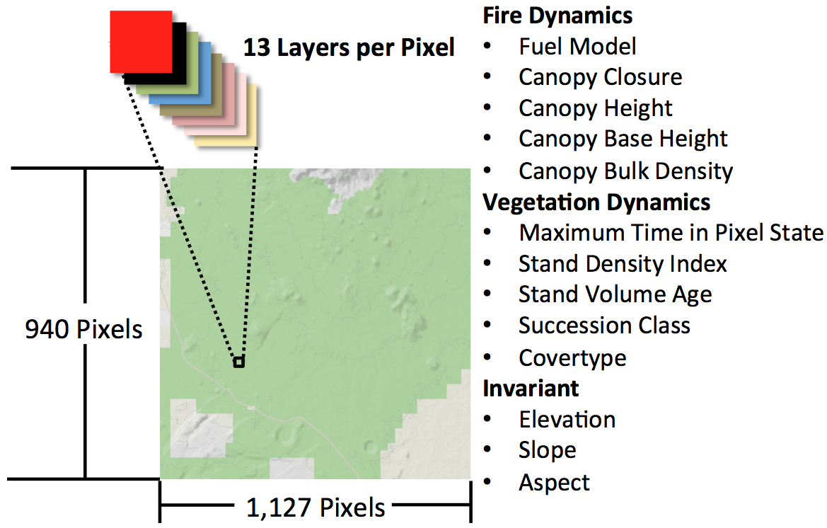
Figure 2: The landscape totals approximately one million pixels, each of which has 13 state variables that influence the spread of wildfire on the landscape. We use summary statistics of the dynamic state variables in MFMC’s distance metric. (Map is copyright of OpenStreetMap contributors)

Figure 2 shows a snapshot of the landscape as generated by the Houtman simulator (Houtman et al., 2013). The landscape is comprised of approximately one million pixels, each with 13 state variables. When a fire is ignited by lightning, the policy must choose between two actions: Suppress (fight the fire) and Let Burn (do nothing). Hence, $|A|=2$.

The simulator spreads wildfires with the FARSITE fire model (Finney, 1998) according to the surrounding pixel variables ($X$) and the hourly weather. Weather variables include hourly wind speed, hourly wind direction, hourly cloud cover, daily maximum/minimum temperature, daily maximum/minimum humidity, daily hour of maximum/minimum temperature, daily precipitation, and daily precipitation duration. These are generated by resampling from 25 years of observed weather (Western Regional Climate Center, 2011). MFMCi can treat the weather variables and the ignition location as exogenous variables because the decision to fight (or not fight) a fire has no influence on weather or ignition locations. Further, changes in the Markov state do not influence the weather or the spatial probability of lightening strikes.

After computing the extent of the wildfire on the landscape, the simulator applies a cached version of the Forest Vegetation Simulator (Dixon, 2002) to update the vegetation of the individual pixels. Finally, a harvest scheduler selects pixels to harvest for timber value.

We constructed three policy classes that map fires to fire suppression decisions. We label these policies intensity, fuel, and location. The intensity policy suppresses fires based on the weather conditions at the time of the ignition and the number of days remaining in the fire season. The fuel policy suppresses fires when the landscape accumulates sufficient high-fuel pixels. The location policy suppresses fires starting on the top half of the landscape, and allows fires on the bottom half of the landscape to burn (which mimics the situation that arises when houses and other buildings occupy part of the landscape). We selected these policy classes because they are functions of different components of the Markov and exogenous state. The intensity policies are a function of the exogenous variables and should be difficult for MFMC because the sequence of actions along a trajectory will be driven primarily by the stochasticity of the weather circumstances. This contrasts with the fuel policy, which should follow the accumulation of vegetation between time steps in the Markov state. Finally, the location policy should produce landscapes that are very different from the other two policy classes as fuels become spatially imbalanced in the Markov state.

The analysis of Fonteneau et al. (2013) assumes the database is populated with state-action transitions covering the entire state-action space. The dimensionality of the wildfire state space makes it impossible to satisfy this assumption. We focus sampling on states likely to be entered by future policy queries by seeding the database with one trajectory for each of 360 policies whose parameters are sampled according to a grid over the intensity policy space. The intensity policy parameters include a measure of the weather conditions at the time of ignition known as the Energy Release Component (ERC) and a measure of the seasonal risk in the form of the calendar day. These measures are drawn from $\big{[}0,100\big{]}$ and $\big{[}0,180\big{]}$, respectively.

The three policy classes are very different from each other. One of our goals is to determine whether MFMCi can use state transitions generated from the intensity policy to accurately simulate state transitions under the fuel and location policies. We evaluate MFMCi by generating 30 trajectories for each policy from the ground truth simulator.

For our distance metric $\Delta_{i}$, we use a weighted Euclidean distance computed over the mean/variance standardized values of the following landscape features: Canopy Closure, Canopy Height, Canopy Base Height, Canopy Bulk Density, Stand Density Index, High Fuel Count, and Stand Volume Age. All of these variables are given a weight of 1. An additional feature, the time step (Year), is added to the distance metric with a very large weight to ensure that MFMCi will only stitch from one state to another if the time steps match. Introducing this non-stationarity ensures we exactly capture landscape growth stages for all pixels that do not experience fire.

Our choice of distance metric features is motivated by the observation that risk profile (the likely size of a wildfire) and vegetation profile (the total tree cover) are easy to capture in low dimensions. If we instead attempt to capture the likely size of a specific fire, we need a distance metric that accounts for the exact spatial distribution of fuels on the landscape. Our distance metric successfully avoids directly modeling spatial complexity.

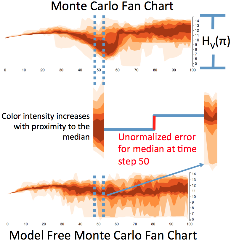
Figure 3: Top: A fan chart generated by Monte Carlo simulations from the expensive simulator. Bottom: A fan chart generated from the MFMC surrogate model. x axis is the time step and y axis is the value of the state variable at each time step. Each change in color shows a quantile boundary for a set of trajectories generated under policy $\pi$. Middle: Error measure is the distance between the median of the Monte Carlo simulations (left) and the median of the MFMC/MFMCi surrogate simulations (right). The error is normalized across fan charts according to $H_{v}(\pi)$, which is the Monte Carlo fan chart height for policy $\pi$ and variable $v$.

To visualize the trajectories, we employ the visualization tool MDPvis (McGregor et al., 2015). The key visualization in MDPvis is the fan chart, which depicts various quantiles of the set of trajectories as a function of time (see Figure 3).

To evaluate the quality of the fan charts generated using surrogate trajectories, we define visual fidelity error in terms of the difference in vertical position between the true median and its position under the surrogate. Specifically, we define $\text{error}(v,t)$ as the offset between the correct location of the median and its MFMCi-modeled location for state variable $v$ in time step $t$. We normalize the error by the height of the fan chart for the rendered policy ($H_{v}(\pi)$). The weighted error is thus $\sum\limits_{v\in S}\sum\limits_{t=0}^{h}\frac{\text{error}(v,t)}{H_{v}(\pi)}$.

This error is measured for 20 variables related to the counts of burned pixels, fire suppression expenses, timber loss, timber harvest, and landscape ecology.

5.1 Experimental Results

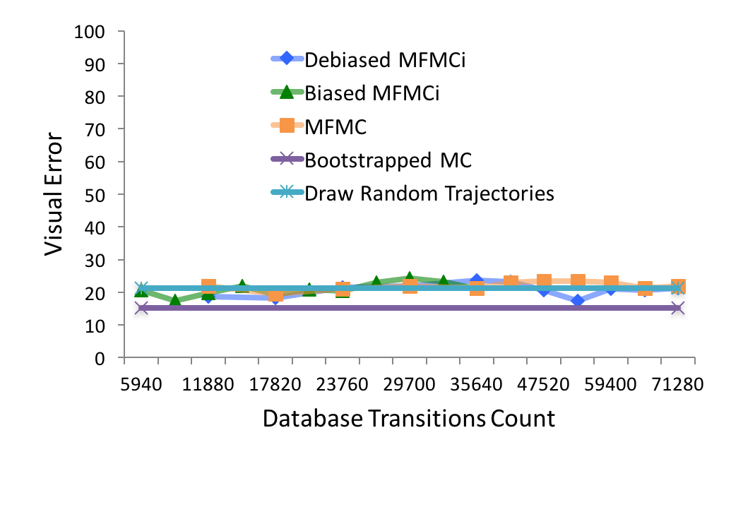
(a) Visual fidelity errors for a weather intensity policy class. Fires are suppressed based on a combination of the weather and how much time is left in the fire season.

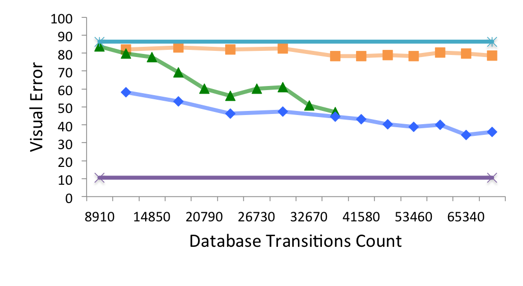
(b) Visual fidelity errors for a ignition location policy class. Fires are always suppressed if they start on the top half of the landscape, otherwise they are always allowed to burn.

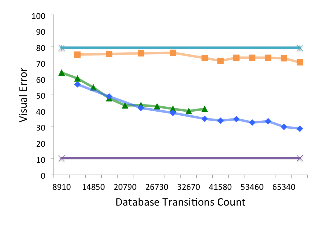
(c) Visual fidelity errors for a fuel accumulation policy class. Fires are always suppressed if the landscape is at least 30 percent in high fuels, otherwise the fire is allowed to burn.

Figure 4: Policy classes for the wildfire domain under a variety of distance metrics and sampling procedures.

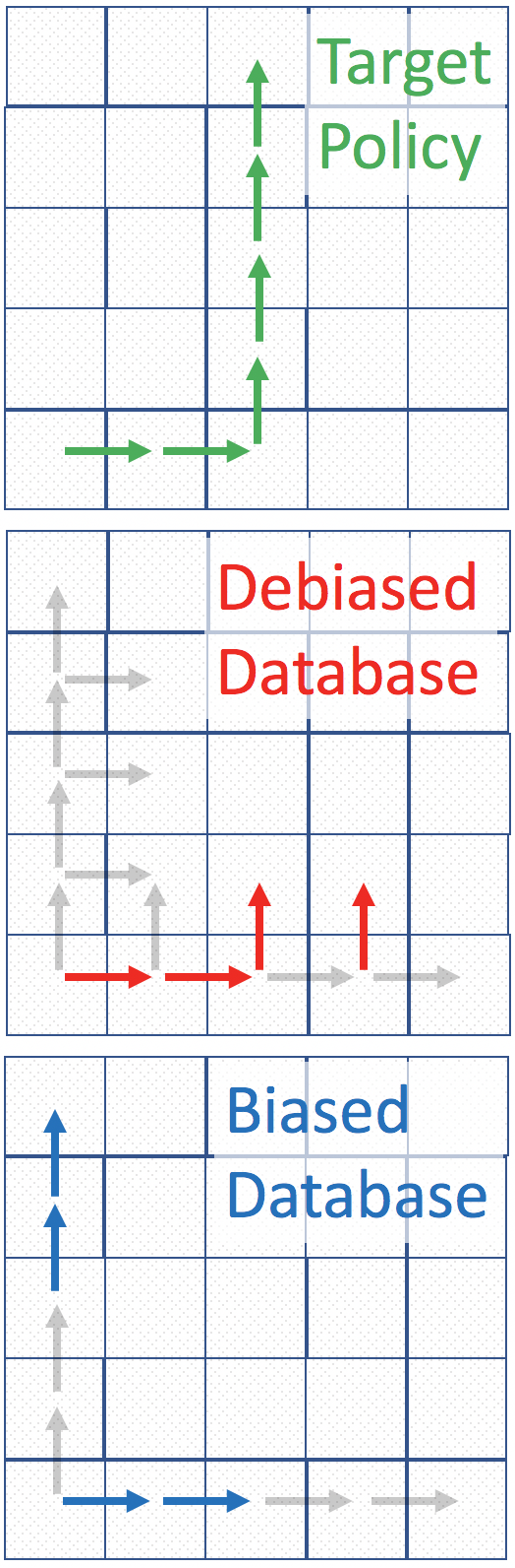
Figure 5: Example of MFMC’s autoregressive tendency for a grid world domain where the only available actions are “up” and “right”. The green arrows show a trajectory that we would like to synthesize from two different MFMC databases where the distance metric is Euclidean with arbitrarily large weight given to the time step and action. The gray arrows show the grid world transitions in the two databases. In the debiased database the stitching operation will stay on the rightward trajectory despite there being transitions that more closely track the target trajectory. The biased database forces the stitching operation to hop to the policy more consistent with the target policy. In some instances it is better to bias the exogenous variables than repeatedly stitch to the same trajectories.

We evaluated the visual fidelity under three settings: (a) debiased MFMCi (exogenous variables excluded from the distance metric $\Delta_{i}$; debiasing tuples included in the database $D$), (b) MFMC (exogenous variables included in $\Delta$), and (c) biased MFMCi (exogenous variables excluded from $\Delta_{i}$ and the extra debiasing tuples removed from $D$). We also compare against two baselines that explore the upper and lower bounds of the visual error. First, we show that the lower bound on visual error is not zero. Although each policy has true quantile values at every time step, estimating these quantiles with 30 trajectories is inherently noisy. We estimate the achievable visual fidelity by bootstrap resampling the 30 ground truth trajectories and report the average visual fidelity error. Second, we check whether the error introduced by stitching is worse than visualizing a set of random database trajectories. Thus the bootstrap resample forms a lower bound on the error, and comparison to the random trajectories detects stitching failure. Figure 4 plots “learning curves” that plot the visualization error as a function of the size of the database $D$. The ideal learning curve should show a rapid decrease in visual fidelity error as $|D|$ grows.

6 Discussion

For each policy class, we chose one target policy from that class and measured how well the behavior of that policy could be simulated by our MFMC variants. Recall that the database of transitions was generated using a range of intensity policies. When we apply the MFMC variants to generate trajectories for an intensity policy, all methods (including random trajectory sampling) produce an accurate representation of the median for MDPvis. When the database trajectories do not match the target policy, MFMCi outperforms MFMC. For some policies, the debiased database outperforms the biased databases, but the difference decreases with additional database samples. Next we explore these findings in more depth.

Intensity Policy. Figure 4(a) shows the results of simulating an intensity policy that suppresses all fires that have an ERC between 75 and 95, and ignite after day 120. This policy suppresses approximately 60 percent of fires. There are many trajectories in the database that agree with the target policy on the majority of fires. Thus, to simulate the target policy it is sufficient to find a policy with a high level of agreement and then sample the entire trajectory. This is exactly what MFMC, MFMCi, and Biased MFMCi do. All of them stitch to a good matching trajectory and then follow it, so they all give accurate visualizations as indicated by the low error rate in Figure 4(a). Unsurprisingly, we can approximate intensity policies from a very small database $D$ built from other intensity policies.

Location Policy. Figure 4(b) plots the visual fidelity error when simulating a location policy from the database of intensity policy trajectories. When $D$ is small, the error is very high. MFMC is unable to reduce this error as $D$ grows, because its distance metric does not find matching fire conditions for similar landscapes. In contrast, because the MFMCi methods are matching on the smaller Markov state variables, they are able to find good matching trajectories. The debiased version of MFMCi outperforms the biased version for the smaller database sizes. In the biased version the matching operation repeatedly stitches over long distances to find a database trajectory with a matching action. Debiased MFMCi avoids this mistake. This explains why debiased MFMCi rapidly decreases the error while biased MFMCi takes a bit longer but then catches up at roughly $|D|=$40,000.

Fuel Policy. The fuel policy shows a best case scenario for the biased database. Within 7 time steps, fuel accumulation causes the policy action to switch from let-burn-all to suppress-all. Since all of the trajectories in the database have a consistent probability of suppressing fires throughout all 100 years, the ideal algorithm will select a trajectory that allows all wildfires to burn for 7 years (to reduce fuel accumulation), then stitch to the most similar trajectory in year 8 that will suppress all future fires. The biased database will perform this “policy switching” by jumping between trajectories to find one that always performs an action consistent with the current policy.

Policy switching is preferable to the debiased database in some cases. To illustrate this, consider the grid world example in Figure 5. It shows that debiased samples can offer stitching opportunities that prevent policy switching and hurt the results.

In summary, our experiments show that MFMCi is able to generalize across policy classes and that it requires only a small number of database trajectories to accurately reproduce the median of each state variable at each future time step. In general, it appears to be better to create a debiased database than a biased database having the same number of tuples.

Our stakeholders in forestry plan to apply the MFMCi surrogate to their task of policy analysis. We demonstrate the effectiveness of the MFMCi surrogate for the problem of wildfire policy optimization in (McGregor et al., 2017).

References

- Abbeel et al. (2005) Abbeel, Pieter, Ganapathi, Varun, and Ng, Andrew Y. Learning Vehicular Dynamics, with Application to Modeling Helicopters. Advances in Neural Information Processing Systems (NIPS), pp. 1–8, 2005. ISSN 1049-5258. URL http://books.nips.cc/nips18.html.
- Arca et al. (2013) Arca, Bachisio, Ghisu, Tiziano, Spataro, William, and Trunfio, Giuseppe a. GPU-accelerated Optimization of Fuel Treatments for Mitigating Wildfire Hazard. Procedia Computer Science, 18:966–975, 2013. ISSN 18770509. doi: 10.1016/j.procs.2013.05.262. URL http://linkinghub.elsevier.com/retrieve/pii/S1877050913004055.
- Bellman (1957) Bellman, Richard. Dynamic Programming. Princeton University Press, New Jersey, 1957.
- Dixon (2002) Dixon, G. Essential FVS : A User’s Guide to the Forest Vegetation Simulator. Number November 2015. USDA Forest Service, Fort Collins, CO, 2002. ISBN 9780903024976. doi: 10.1007/978-3-319-23883-8.
- Finney (1998) Finney, Mark A. FARSITE: fire area simulator – model development and evaluation. USDA Forest Service, Rocky Mountain Research Station, Missoula, MT, 1998.
- Fonteneau & Prashanth (2014) Fonteneau, Raphael and Prashanth, L A. Simultaneous Perturbation Algorithms for Batch Off-Policy Search. In 53rd IEEE Conference on Conference on Decision and Control, 2014.
- Fonteneau et al. (2010) Fonteneau, Raphael, Murphy, Susan A, Wehenkel, Louis, and Ernst, Damien. Model-Free Monte Carlo-like Policy Evaluation. Proceedings of the Thirteenth International Conference on Artificial Intelligence and Statistics (AISTATS 2010), pp. 217–224, 2010.
- Fonteneau et al. (2013) Fonteneau, Raphael, Murphy, Susan a, Wehenkel, Louis, and Ernst, Damien. Batch Mode Reinforcement Learning based on the Synthesis of Artificial Trajectories. Annals of Operations Research, 208(1):383–416, Sep 2013. ISSN 0254-5330. doi: 10.1007/s10479-012-1248-5. URL http://www.pubmedcentral.nih.gov/articlerender.fcgi?artid=3773886&tool=pmcentrez&rendertype=abstract.
- Houtman et al. (2013) Houtman, Rachel M., Montgomery, Claire A., Gagnon, Aaron R., Calkin, David E., Dietterich, Thomas G., McGregor, Sean, and Crowley, Mark. Allowing a Wildfire to Burn: Estimating the Effect on Future Fire Suppression Costs. International Journal of Wildland Fire, 22(7):871–882, 2013.
- McGregor et al. (2015) McGregor, Sean, Buckingham, Hailey, Dietterich, Thomas G., Houtman, Rachel, Montgomery, Claire, and Metoyer, Ron. Facilitating Testing and Debugging of Markov Decision Processes with Interactive Visualization. In IEEE Symposium on Visual Languages and Human-Centric Computing, Atlanta, 2015.
- McGregor et al. (2017) McGregor, Sean, Houtman, Rachel, Montgomery, Claire, Metoyer, Ronald, and Dietterich, Thomas G. Fast Optimization of Wildfire Suppression Policies with SMAC. ArXiv, 2017. URL https://arxiv.org/abs/1703.09391.
- Puterman (1994) Puterman, Martin. Markov Decision Processes: Discrete Stochastic Dynamic Programming. Wiley-Interscience, 1st edition, 1994.
- Sutton (1990) Sutton, Richard S. Integrated architectures for learning, planning, and reacting based on approximating dynamic programming. In Proceedings of the Seventh International Conference on Machine Learning, pp. 216–225, San Francisco, CA, 1990. Morgan Kaufmann.
- Western Regional Climate Center (2011) Western Regional Climate Center. Remote Automated Weather Stations (RAWS). Western Regional Climate Center, Reno, NV, 2011.