Parameter estimation for fractional Ornstein-Uhlenbeck processes of general Hurst parameter

Abstract

This paper provides several statistical estimators for the drift and volatility parameters of an Ornstein-Uhlenbeck process driven by fractional Brownian motion, whose observations can be made either continuously or at discrete time instants. First and higher order power variations are used to estimate the volatility parameter. The almost sure convergence of the estimators and the corresponding central limit theorems are obtained for all the Hurst parameter range $H\in(0,1)$. The least squares estimator is used for the drift parameter. A central limit theorem is proved when the Hurst parameter $H\in(0,1/2)$ and a noncentral limit theorem is proved for $H\in[3/4,1)$. Thus, the open problem left in the previous paper [11] is completely solved, where a central limit theorem for least squares estimator is proved for $H\in[1/2,3/4)$.

1 Introduction

Consider the fractional Ornstein-Uhlenbeck process defined as the unique pathwise solution to the stochastic differential equation

$$dX_{t}=-\theta X_{t}dt+\sigma_{t}dB_{t}^{H}\,,$$ (1.1)

with initial condition $X_{0}\in\mathbb{R}$, where $B^{H}=\{B^{H}_{t},t\geq 0\}$ is a fractional Brownian (fBm) motion of Hurst parameter $H\in(0,1)$, $\theta$ is a positive parameter and the volatility ${\sigma}_{t}$ is a stochastic process with $\beta$-Hölder continuous trajectories, where $\beta>1-H$. Under this condition on ${\sigma}_{t}$, the stochastic integral $\int_{0}^{t}\sigma_{s}dB^{H}_{s}$ is well defined as a pathwise Riemann-Stieljes integral (see, for instance, [26]) and the above stochastic differential equation has a unique solution.

Assume that the parameters ${\theta}>0$ and ${\sigma}_{t}$ are unknown and that the process can be observed continuously or at discrete time instants. We want to estimate the integrated volatility $\int_{0}^{t}|{\sigma}_{s}|^{p}ds$ and the drift parameter $\theta$ for any $H\in(0,1)$. We assume that the Hurst parameter $H$ is known or it can be estimated by other methods (for example, see [5] and the references therein).

In the paper [10], Nualart, Corcuera and Woerner studied the asymptotic behavior of the power variation of the stochastic integral $Z_{t}=\int^{t}_{0}u_{s}dB^{H}_{s}$, defined as $V^{n}_{p}(Z)_{t}=\sum^{[nt]}_{i=1}|Z_{i/n}-Z_{(i-1)/n}|^{p}$ for any $p>0$. They proved that if the process $u=\{u_{t},t\geq 0\}$ has finite $q$-variation on any finite interval, for some $q<1/(1-H)$, then, as $n\rightarrow\infty$,

$$n^{-1+pH}V^{n}_{p}(Z)_{t}\rightarrow c_{1,p}\int_{0}^{t}|u_{s}|^{p}ds$$

uniformly in probability in any compact sets of $t$, where $c_{1,p}=\mathbb{E}[|B^{H}_{1}|^{p}]$. The corresponding central limit theorem was also obtained for $H\in(0,\frac{3}{4}]$. These results can be applied to construct an estimator based on the power variation of $\int_{0}^{t}\sigma_{s}dB^{H}_{s}$ to estimate the integrated volatility $\int_{0}^{t}|{\sigma}_{s}|^{p}ds$ when $H\in(0,\frac{3}{4}]$. However, the condition $H\in(0,\frac{3}{4}]$ is critical in [10]. The first objective of this paper is to remove this restriction. To this end, we shall use higher order power variations defined as $V^{n}_{k,p}(Z)_{t}=\sum^{[nt]-k+1}_{i=1}\left|\sum_{j=0}^{k}(-1)^{k-j}{\left({k}\atop{j}\right)}Z_{(i+j-1)/n}\right|^{p}$, for any integer $k\geq 1$. In Section 3, we study the asymptotic behavior of these higher order power variations of the general stochastic integral $Z_{t}=\int_{0}^{t}u_{s}dB_{s}^{H}$. The application of these results to estimate the integrated volatility are presented in Section 4. In particular, when ${\sigma}_{t}={\sigma}$ we can use $\displaystyle\left|\hat{\sigma}_{T}\right|^{p}=\displaystyle\frac{n^{-1+pH}V^{n}_{k,p}(X)_{T}}{c_{k,p}T}$ to estimate ${\sigma}$, where $c_{k,p}$ is the constant introduced in (3.1). The uniform convergence in probability and central limit theorems of the estimators for both the integrated volatility and the volatility itself are established.

It is worth mentioning that the statistical estimation of the integrated volatility has already been studied in the recent decades. Barndorff-Nielsen et al [1] - [3]) studied estimation of volatility for Brownian semimartingale and Brownian semi-stationary processes by using power, bipower, or multipower variations. However, those results cannot be applied to the fractional Ornstein-Uhlenbeck process due to its lack of the semimartingale property.

As for the drift parameter $\theta$, several estimators have been proposed previously. A summary of some relevant results are presented below.

(i)

In the case of continuous observations, Kleptsyna and Le Breton ([13]) studied the maximum likelihood estimator (MLE) which is defined by

$$\hat{\theta}_{MLE}=-\left\{\int_{0}^{T}Q^{2}(s)dw_{s}^{H}\right\}^{-1}\int_{0}^{T}Q(s)dZ_{s}\,,$$

where

$$Q(t)=\frac{d}{dw_{t}^{H}}\int_{0}^{t}k_{H}(t,s)X_{s}ds,\quad Z_{t}=\int_{0}^{t}k_{H}(t,s)dX_{s},$$

$k_{H}(t,s)=\kappa_{H}^{-1}s^{\frac{1}{2}-H}(t-s)^{\frac{1}{2}-H}$ and $w_{t}^{H}=\lambda_{H}^{-1}t^{2-2H}$ with constants $\kappa_{H}$ and $\lambda_{H}$ depending on $H$. They proved the almost sure convergence of $\hat{\theta}_{MLE}$ to $\theta$ as $T$ tends to infinity. It is worth noting that Tudor and Viens ([24]) have also obtained the almost sure convergence of both the MLE and a version of the MLE using discrete observations for all $H\in(0,1)$. Bercu, Courtin and Savy proved in [4] the following central limit theorem for the MLE in the case of $H>\frac{1}{2}$:

$$\sqrt{T}(\hat{\theta}_{MLE}-\theta)\xrightarrow[T\to\infty]{\mathcal{L}}N(0,2\theta)\,.$$

They claimed without proof that the above convergence is also valid for $H\in(0,\frac{1}{2})$.

(ii)

On the other hand, Hu and Nualart ([11]) proposed the least square estimator defined by

$$\hat{\theta}_{T}=-\displaystyle\frac{\int^{T}_{0}X_{t}dX_{t}}{\int^{T}_{0}X_{t}^{2}dt}=\theta-\sigma\frac{\int^{T}_{0}X_{t}dB_{t}^{H}}{\int^{T}_{0}X_{t}^{2}dt}\,,$$ (1.2)

where the integral with respect to $B^{H}$ is interpreted in the Skorohod sense. They also introduced another estimator $\widetilde{\theta}_{T}$ based on the ergodic theorem given by

$$\widetilde{\theta}_{T}=\Big{(}\displaystyle\frac{1}{\sigma^{2}H\Gamma(2H)T}\int^{T}_{0}X^{2}_{t}dt\Big{)}^{-\frac{1}{2H}}\,.$$ (1.3)

Almost sure convergence and central limit theorems for these two estimators have been proved for $H\in[\frac{1}{2},\frac{3}{4})$.

However, when $H\in(0,\frac{1}{2})\cup[\frac{3}{4},1)$, the central limit theorems for the least square estimator $\hat{\theta}_{T}$ have not been known yet. The first objective of Section 5 is to prove the asymptotic consistency of $\hat{\theta}_{T}$ by using a new method, different from that in [11], which is valid for all $H\in(0,1)$. This method involves the relationship between the divergence and Stratonovich integrals and the integration by parts technique and it is based on the pathwise properties of the fractional Ornstein-Uhlenbeck process established in a paper [7] by Cheridito, Kawaguchi and Maejima. The next and the main objective of this paper is to establish a central limit theorem for the least square estimator $\hat{\theta}_{T}$ for $H\in(0,\frac{1}{2})$ and a noncentral limit theorem for $H\in[\frac{3}{4},1)$. In the later case, we can identify the limit as a Rosenblatt random variable. We will make a comparison of the asymptotic variance for these three estimators and show that the least square estimator performs better than the maximum likelihood estimator when $H\in(0,\frac{1}{2})$. Since the ergodic-type estimator $\widetilde{\theta}_{T}$ is a function of a pathwise Riemann integral that appears simpler than the other two estimators, we will use $\widetilde{\theta}_{T}$ to construct a consistent estimator $\bar{\theta}_{n}$ for high frequency data (if only discrete observations are available). The asymptotic behavior of $\bar{\theta}_{n}$ in this case is also studied in this paper. The proofs of our results are highly technical and rely on some sophisticated computation, which we shall put in the Appendix. The main tool we use is Malliavin calculus which is recalled in Section 2. We use $C$ to denote a generic constant that may vary according to the context.

2 Preliminaries

In this section, we briefly recall some notions and results on fractional Brownian motion, $p$-variation, and Malliavin calculus.

The fractional Brownian motion (fBm) $B^{H}=\{B^{H}_{t},t\in\mathbb{R}\}$ with Hurst parameter $H\in(0,1)$ is a zero mean Gaussian process, defined on a complete probability space $(\Omega,\mathcal{F},P)$, with the following covariance function

$$\mathbb{E}(B^{H}_{t}B^{H}_{s})=R_{H}(t,s)=\frac{1}{2}(|t|^{2H}+|s|^{2H}-|t-s|^{2H}).$$ (2.1)

From (2.1), it is easy to see that $\mathbb{E}|B_{t}^{H}-B_{s}^{H}|^{2}=|t-s|^{2H}$. Then it follows from Kolmogorov’s continuity criterion that on any finite interval, almost surely all paths of fBm are $\alpha$-Hölder continuous with $\alpha<H$. Denote by $\eta_{T}$ the $\alpha$-Hölder coefficient of fBm on the interval $[0,T]$, i.e.,

$$\eta_{T}=\sup_{t\neq s\in[0,T]}\frac{\left|B_{t}^{H}-B_{s}^{H}\right|}{|t-s|^{\alpha}}\,.$$ (2.2)

Clearly, $\mathbb{E}|\eta_{T}|^{q}=T^{q(H-\alpha)}\mathbb{E}|\eta_{1}|^{q}$ for any $q>1$, by the self-similarity property of fBm.

Let $\mathcal{F}$ denote the $\sigma$-field obtained from the completion of the $\sigma$-field generated by $B^{H}$. Let $\mathcal{E}$ denote the space of all real valued step functions on $\mathbb{R}$. The Hilbert space $\mathfrak{H}$ is defined as the closure of $\mathcal{E}$ endowed with the inner product

$$\langle\mathbf{1}_{[a,b]},\mathbf{1}_{[c,d]}\rangle_{\mathfrak{H}}=\mathbb{E}\left((B_{b}^{H}-B_{a}^{H})(B_{d}^{H}-B_{c}^{H})\right)\,.$$

Under the convention that $\mathbf{1}_{[0,t]}=-\mathbf{1}_{[t,0]}$ if $t<0$, the mapping $\mathbf{1}_{[0,t]}\mapsto B^{H}_{t}$ can be extended to a linear isometry between $\mathfrak{H}$ and the Gaussian space $\mathcal{H}_{1}$ spanned by $B^{H}$. We denote this isometry by $\mathfrak{H}\ni\varphi\mapsto B^{H}(\varphi)$. If $f,g\in\mathfrak{H}$ and $g$ is a continuously differentiable function with compact support, we can use step functions in $\mathcal{E}$ to approximate $f$ and $g$ and by a limiting argument we deduce

$$\langle f,g\rangle_{\mathfrak{H}}=\int_{\mathbb{R}^{2}}f(t)g^{\prime}(s)\frac{\partial R_{H}(t,s)}{\partial t}dtds$$ (2.3)

(see [12]). We can also use Fourier transform to compute $\langle f,g\rangle_{\mathfrak{H}}$, namely,

$$\langle f,g\rangle_{\mathfrak{H}}=\frac{1}{c_{H}^{2}}\int_{\mathbb{R}}\mathcal{F}f(\xi)\overline{\mathcal{F}g(\xi)}|\xi|^{1-2H}d\xi,$$ (2.4)

where $c_{H}=\Big{(}\frac{2\pi}{\Gamma(2H+1)\sin(\pi H)}\Big{)}^{\frac{1}{2}}$ (see [23]). When $H>1/2$, for any $f,g\in L^{1/H}([0,T])$, if we extend $f$ and $g$ to be zero on $\mathbb{R}\cap[0,T]^{c}$, then $f,g\in\mathfrak{H}$ and we have the following simple identity

$$\langle f,g\rangle_{\mathfrak{H}}=\alpha_{H}\int_{[0,T]^{2}}f(u)g(v)|u-v|^{2H-2}dudv\,,$$ (2.5)

where $\alpha_{H}=H(2H-1)$.

For any $p>0$, the $p$-variation of a real-valued function $f$ on an interval $[a,b]$ is defined as

$${\rm var}_{p}(f;[a,b])={\rm sup}_{\pi}\Big{(}\sum_{i=1}^{n}|f(t_{i})-f(t_{i-1})|^{p}\Big{)}^{1/p}\,,$$

where the supremum runs over all partitions $\pi=\{a=t_{0}<t_{1}<\cdots<t_{n}=b\}$. If $f$ is $\alpha$-Hölder continuous on the interval $[a,b]$, $\alpha\in(0,1]$, then we set

$$\|f\|_{\alpha}:={\rm sup}_{a\leq s<t\leq b}\frac{|f(t)-f(s)|}{|t-s|^{\alpha}}\,.$$

It is known that an $\alpha$ -Hölder continuous function $f$ on the interval $[a,b]$ has finite $1/\alpha$-variation on this interval. If $f$ and $g$ have finite $p$-variation and finite $q$-variation on the interval $[a,b]$ respectively and $1/p+1/q>1$, the Riemann-Stieltjes integral $\int_{a}^{b}fdg$ exists (see Young [26]). By Young’s result, the stochastic integral $\int_{0}^{t}u_{s}dB_{s}^{H}$ is well defined as a pathwise Riemann-Stieltjes integral provided that the trajectories of the process $\{u_{t},t\geq 0\}$ have finite $q$-variation on any finite interval for some $q<1/(1-H).$

Next we define two types of stochastic integrals: Stratonovich integral and divergence integral. Given a stochastic process $\{v(t),t\geq 0\}$ such that $\int_{0}^{t}|v(s)|ds<\infty$ a.s. for all $t>0$, the Stratonovich integral $\int_{0}^{t}v(s)\circ dB_{s}^{H}$ is defined as the following limit in probability if it exists

$$\lim_{\epsilon\to 0}\int_{0}^{t}v(s)\dot{B}_{s}^{H,{\varepsilon}}ds\,,$$

where $\dot{B}_{s}^{H,{\varepsilon}}$ is a symmetric approximation of $\dot{B}_{s}^{H}$:

$$\dot{B}_{s}^{H,{\varepsilon}}=\frac{1}{2\epsilon}(B_{s+\epsilon}^{H}-B_{s-\epsilon}^{H})\,.$$

Before we define the divergence integral, we present some background of Malliavin calculus. For a smooth and cylindrical random variable $F=f(B^{H}(\varphi_{1}),\dots,B^{H}(\varphi_{n}))$, with $\varphi_{i}\in\mathfrak{H}$ and $f\in C_{b}^{\infty}(\mathbb{R}^{n})$ ($f$ and all of its partial derivatives are bounded), we define its Malliavin derivative as the $\mathfrak{H}$-valued random variable given by

$$DF=\sum_{i=1}^{n}\frac{\partial f}{\partial x_{i}}(B^{H}(\varphi_{1}),\dots,B^{H}(\varphi_{n}))\varphi_{i}.$$

By iteration, one can define the $k$-th derivative $D^{k}F$ as an element of $L^{2}(\Omega;\mathfrak{H}^{\otimes k})$. For any natural number $k$ and any real number $p\geq 1$, we define the Sobolev space $\mathbb{D}^{k,p}$ as the closure of the space of smooth and cylindrical random variables with respect to the norm $||\cdot||_{k,p}$ defined by

$$||F||^{p}_{k,p}=\mathbb{E}(|F|^{p})+\sum_{i=1}^{k}\mathbb{E}(||D^{i}F||^{p}_{\mathfrak{H}^{\otimes i}}).$$

The divergence operator $\delta$ is defined as the adjoint of the derivative operator $D$ in the following manner. An element $u\in L^{2}(\Omega;\mathfrak{H})$ belongs to the domain of $\delta$, denoted by ${\rm Dom}\,\delta$, if there is a constant $c_{u}$ depending on $u$ such that

$$|\mathbb{E}(\langle DF,u\rangle_{\mathfrak{H}})|\leq c_{u}||F||_{L^{2}(\Omega)}$$

for any $F\in\mathbb{D}^{1,2}$. If $u\in{\rm Dom}\,\delta$, then the random variable $\delta(u)$ is defined by the duality relationship

$$\mathbb{E}(F\delta(u))=\mathbb{E}(\langle DF,u\rangle_{\mathfrak{H}})\,,$$

which holds for any $F\in\mathbb{D}^{1,2}$. If $u=\{u_{t},t\in[0,T]\}$ is a stochastic process, whose trajectories belong to $\mathfrak{H}$ almost surely (with the convention $u_{t}=0$ if $t\not\in[0,T]$) and $u\in{\rm Dom}\,\delta$, we make use of the notation $\int_{0}^{T}u_{t}dB_{t}^{H}=\delta(u)$ and call $\delta(u)$ the divergence integral of $u$ with respect to the fractional Brownian motion $B^{H}$ on $[0,T]$. It is worth noting that the divergence integral of fBm with respect to itself does not exist if $H\in(0,\frac{1}{4})$ because the paths of the fBm are too irregular (see [8]). For this reason, in [8] the authors introduce an extended divergence integral $\delta^{*}$ such that ${\rm Dom}\,\delta^{*}\cap L^{2}(\Omega;\mathfrak{H})={\rm Dom}\,\delta$ and the extended divergence operator $\delta^{*}$ restricted to ${\rm Dom}\,\delta$ coincides with the divergence operator. In a similar way we can introduce the iterated divergence operator $\delta^{k}$ for each integer $k\geq 2$, defined by the duality relationship

$$\mathbb{E}(F\delta^{k}(u))=\mathbb{E}\left(\langle D^{k}F,u\rangle_{\mathfrak{H}^{\otimes k}}\right)\,,$$

for any $F\in\mathbb{D}^{k,2}$, where $u\in{\rm Dom}\,\delta^{k}\subset L^{2}(\Omega;\mathfrak{H}^{\otimes k})$.

For any integer $m\geq 1$, we use $\mathfrak{H}^{\otimes m}$ and $\mathfrak{H}^{\odot m}$ to denote the $m$-th tensor product and the $m$-th symmetric tensor product of the Hilbert space $\mathfrak{H}$, respectively. We denote by $\mathcal{H}_{m}$ the closed linear subspace of $L^{2}(\Omega)$ generated by the random variables $\{H_{m}(B^{H}(\varphi)):\varphi\in\mathfrak{H},||\varphi||_{\mathfrak{H}}=1\}$, where $H_{m}$ is the $m$-th Hermite polynomial defined by

$$H_{m}(x)=\frac{(-1)^{m}}{m!}e^{\frac{x^{2}}{2}}\frac{d^{m}}{dx^{m}}e^{-\frac{x^{2}}{2}},\quad m\geq 1,$$

and $H_{0}(x)=1$. The space $\mathcal{H}_{m}$ is called the Wiener chaos of order $m$. The $m$-th multiple integral of $\varphi\in\mathfrak{H}^{\odot m}$ is defined by the identity $I_{m}(\varphi)=\delta^{m}(\varphi)$, and in particular, $I_{m}(\phi^{\otimes m})=H_{m}(B^{H}(\phi))$ for any $\phi\in\mathfrak{H}$. The map $I_{m}$ provides a linear isometry between $\mathfrak{H}^{\odot m}$(equipped with the norm $\frac{1}{\sqrt{m!}}||\cdot||_{\mathfrak{H}^{\otimes m}}$) and $\mathcal{H}_{m}$ (equipped with $L^{2}(\Omega)$ norm) (see [20], Theorem 2.7.7). By convention, $\mathcal{H}_{0}=\mathbb{R}$ and $I_{0}(x)=x$.

Let us recall the definition of the Rosenblatt process that will appear in the the limit theorems of Section 5. Fix $H>3/4$ and $t\in[0,1]$. Consider the sequence of functions of two variables

$$\xi_{n,t}=2^{n}\sum\limits_{i=1}^{[2^{n}t]}{\bf 1}_{((i-1)2^{-n},i2^{-n}]}^{\otimes 2}\,.$$

Through a direct computation using (2.5) one can show that this sequence is Cauchy in $\mathfrak{H}^{\otimes{2}}$ and converges to distribution denoted by $\delta_{0,t}$ and defined by

$$\langle\delta_{0,t},f\rangle=\int_{0}^{t}f(s,s)ds,$$ (2.6)

for any test function $f$ on $\mathbb{R}^{2}$. It turns out (see [15] for the proofs) that the sequence $I_{2}(\xi_{n,t})$ converges in $L^{2}$ as $n$ tends to infinity to the Rosenblatt random variable $R_{t}=I_{2}(\delta_{0,t})$. For any $f\in L^{1/H}([0,1]^{2})$, we have the following formula, letting $f$ equal to zero on $\mathbb{R}^{2}\cap[0,1]^{c}$,

$$\mathbb{E}(R_{t}I_{2}(f))=2\langle\delta_{0,t},f\rangle_{\mathfrak{H}^{\otimes 2}}=2\alpha_{H}^{2}\int_{0}^{t}dv\int_{[0,1]^{2}}f(u_{1},u_{2})|u_{1}-v|^{2H-2}|u_{2}-v|^{2H-2}du_{1}du_{2}\,.$$ (2.7)

The space $L^{2}(\Omega)$ can be decomposed into the infinite orthogonal sum of the spaces $\mathcal{H}_{m}$, which is known as the Wiener chaos expansion. Thus, any square integrable random variable $F\in L^{2}(\Omega)$ has the following expansion,

$$F=\sum_{m=0}^{\infty}I_{m}(f_{m}),$$

where $f_{0}=\mathbb{E}(F)$, and $f_{m}\in\mathfrak{H}^{\odot m}$ are uniquely determined by $F$. We denote by $J_{m}$ the orthogonal projection onto the $m$-th Wiener chaos $\mathcal{H}_{m}$. This means that $I_{m}(f_{m})=J_{m}(F)$ for every $m\geq 0$.

Let $\{e_{k},k\geq 1\}$ be a complete orthonormal system in the Hilbert space $\mathfrak{H}$. Given $f\in\mathfrak{H}^{\odot n},g\in\mathfrak{H}^{\odot m}$, and $p=1,\dots,n\wedge m$, the $p$-th contraction between $f$ and $g$ is the element of $\mathfrak{H}^{\otimes(m+n-2p)}$ defined by

$$f\otimes_{p}g=\sum_{i_{1},\dots,i_{p}=1}^{\infty}\langle f,e_{i_{1}}\otimes\cdots\otimes e_{i_{p}}\rangle_{\mathfrak{H}^{\otimes p}}\otimes\langle g,e_{i_{1}}\otimes\cdots\otimes e_{i_{p}}\rangle_{\mathfrak{H}^{\otimes p}}\,.$$

The following result (known as the fourth moment theorem) provides necessary and sufficient conditions for the convergence of some random variables to a normal distribution (see [17, 18, 20]).

Theorem 2.1.

Let $n\geq 2$ be a fixed integer. Consider a collection of elements $\{f_{T},T>0\}$ such that $f_{T}\in\mathfrak{H}^{\odot n}$ for every $T>0$. Assume further that

$$\lim_{T\to\infty}\mathbb{E}[I_{n}(f_{T})^{2}]=\lim_{T\to\infty}n!\|f_{T}\|^{2}_{\mathfrak{H}^{\otimes{n}}}=\sigma^{2}.$$

Then the following conditions are equivalent:

1. $\lim_{T\to\infty}\mathbb{E}[I_{n}(f_{T})^{4}]=3\sigma^{2}$.

2. For every $p=1,\dots,n-1$, $\lim_{T\to\infty}||f_{T}\otimes_{p}f_{T}||_{\mathfrak{H}^{\otimes 2(n-p)}}=0$.

3. As $T$ tends to infinity, the $n$-th multiple integrals $\{I_{n}(f_{T}),T\geq 0\}$ converge in distribution to a standard Gaussian random variable $N(0,\sigma^{2})$.

4. $\|D(I_{n}(f_{T}))\|_{\mathfrak{H}}^{2}\xrightarrow[T\to\infty]{L^{2}(\Omega)}n\sigma^{2}$.

Remark 2.2.

The multidimensional version of the above theorem is also stated and proved in [17, 20, 21].

In the paper [17], Nualart and Ortiz-Lattore apply the fourth moment theorem to establish the following weak convergence result for an arbitrary sequence of centered square integrable random vectors.

Theorem 2.3.

Let $\{F_{k},k\in\mathbb{N}\}$ be a sequence of $d$-dimensional centered square integrable random vectors with the following Wiener chaos expansions:

$$F_{k}=\sum_{m=1}^{\infty}J_{m}F_{k}\,.$$

Suppose that:

• $\lim_{M\to\infty}\limsup_{k\to\infty}\sum_{m=M+1}^{\infty}\mathbb{E}[|J_{m}F_{k}|^{2}]=0$ .

• For every $m\geq 1$, $1\leq i,j\leq d$, $\lim_{k\to\infty}\mathbb{E}[(J_{m}F_{k}^{i})(J_{m}F_{k}^{j})]=C_{m}^{ij}$.

• For all $v\in\mathbb{R}^{d}$, $\sum_{m=1}^{\infty}v^{T}C_{m}v=v^{T}Cv$, where $C$ is a $d\times d$ symmetric nonnegative definite matrix.

• For all $m\geq 1$, $1\leq i,j\leq d$,

  $$\langle D(J_{m}F_{k}^{i}),D(J_{m}F_{k}^{j})\rangle_{\mathfrak{H}}\xrightarrow[k\to\infty]{L^{2}(\Omega)}mC_{m}^{ij}\,.$$

Then, $F_{k}$ converges in distribution to the $d$-dimensional normal law $N_{d}(0,C)$ as $k$ tends to infinity.

We end this section by stating the following theorem proved in the paper [9] on the asymptotic behavior of weighted random sums. It will be used in the next section to prove the central limit theorem of the power variation of stochastic integrals.

Theorem 2.4.

Let $(\Omega,\mathcal{F},P)$ be a complete probability space. Fix a time interval $[0,T]$ and consider a double sequence of random variables $\xi=\{\xi_{i,m},m\in\mathbb{Z}_{+},1\leq i\leq[mT]\}$. Assume the double sequence $\xi$ satisfies the following hypotheses.
(H1) Denote $g_{m}(t):=\sum_{i=1}^{[mt]}\xi_{i,m}$. The finite dimensional distributions of the sequence of processes $\{g_{m}(t),t\in[0,T]\}$ converges $\mathcal{F}$-stably to those of $\{B(t),t\in[0,T]\}$ as $m\to\infty$, where $\{B(t),t\in[0,T]\}$ is a standard Brownian motion independent of $\mathcal{F}$.
(H2) $\xi$ satisfies the tightness condition $\mathbb{E}\left|\sum_{i=j+1}^{k}\xi_{i,m}\right|^{4}\leq C\left(\frac{k-j}{m}\right)^{2}$ for any $1\leq j<k\leq[mT]$.
If $\{f(t),t\in[0,T]\}$ is an $\alpha-$Hölder continuous process with $\alpha>1/2$ and we set $X_{m}(t):=\sum_{i=1}^{[mt]}f(\frac{i}{m})\xi_{i,m}$, then we have the $\mathcal{F}$-stable convergence

$$X_{m}(t)\xrightarrow[m\to\infty]{\mathcal{L}}\int_{0}^{t}f(s)dB(s),$$

in the Skorohod space $\mathcal{D}[0,T]$.

3 Asymptotic behavior of power variation

In this section, we introduce high order power variations and prove some asymptotic results for the high order power variations of stochastic integrals with respect to fBm. The high order power variations will be used to construct estimators for the volatility and the integrated volatility of fractional Ornstein-Uhlenbeck processes in the next section.

Consider a sequence of random variables $\{X_{i-1}\,,i\geq 1\}$. Denote the first order difference $\Delta X_{i-1}=\Delta_{1}X_{i-1}=X_{i}-X_{i-1}$. Define the $k$-th order difference by induction as follows $\Delta_{k}X_{i-1}=\Delta_{k-1}X_{i}-\Delta_{k-1}X_{i-1}$ for $k=2,3,\dots$, namely,

$$\Delta_{k}X_{i-1}=\sum_{j=0}^{k}(-1)^{k-j}{\left({k}\atop{j}\right)}X_{i+j-1}\,.$$

Let $B^{H}=\{B^{H}_{t},t\geq 0\}$ be a fBm with Hurst parameter $H\in(0,1)$. For any $j\geq 0$, we can write down the covariance function of the $k$-th order difference of the sequences $\{B^{H}_{n},n\geq 0\}$ and $\{B^{H}_{n+j},n\geq 0\}$ as follows

$$\rho_{k,H}(j):=\mathbb{E}[(\Delta_{k}B^{H}_{n+j})(\Delta_{k}B^{H}_{n})]=\frac{1}{2}\sum_{i=-k}^{k}(-1)^{1-i}\dbinom{2k}{k-i}|j-i|^{2H}\,.$$

Since all the moments of a mean zero Gaussian can be expressed by its variance, we see that the $p$-th moment of $\Delta_{k}B^{H}_{n}$ is given by

$$c_{k,p}=\mathbb{E}[|\Delta_{k}B_{n}^{H}|^{p}]=\displaystyle\frac{2^{p/2}\Gamma((p+1)/2)}{\Gamma(1/2)}[\rho_{k,H}(0)]^{p/2}.$$ (3.1)

Notice that the quantities $\rho_{k,H}(j)$ and $c_{k,p}$ are independent of $n$, due to the fact that the fBm has stationary increments.

From the fact that $\rho_{k,H}(j)=o(j^{2H-2k})$ for $j$ large it follows that

$$\sum_{j=0}^{\infty}\rho_{k,H}^{2}(j)\begin{cases}=\infty&\qquad\hbox{when $k=1$ and $\frac{3}{4}\leq H<1$},\\ <\infty&\qquad\hbox{when $k=1$ and when $0<H<\frac{3}{4}$},\\ <\infty&\qquad\hbox{when $k\geq 2$}\,.\end{cases}$$

Let $p>0$ and let $n\geq 1$ be an integer. We define the $k$-th order $p$-variation of a stochastic process $Z=\{Z_{t},t\geq 0\}$ as

$$V^{n}_{k,p}(Z)_{t}=\sum^{[nt]-k+1}_{i=1}|\Delta_{k}Z_{\frac{i-1}{n}}|^{p}=\sum^{[nt]-k+1}_{i=1}\left|\sum_{j=0}^{k}(-1)^{k-j}{\left({k}\atop{j}\right)}Z_{\frac{i+j-1}{n}}\right|^{p}\,,$$ (3.2)

where we use the convention that the sum is zero if $[nt]-k+1<1$.

The following proposition shows the convergence of the $k$-th order $p$-variation for stochastic integrals of fractional Brownian motion, extending a result in [10] which is valid when $k=1$.

Theorem 3.1.

Let $k\geq 2$ and let $H\in(0,1)$. Suppose that $\{u_{t},t\in[0,T]\}$ is a stochastic process whose sample paths are Hölder continuous with exponent $1/q$ for a certain $q<\frac{1}{1-H}$. Consider the pathwise Riemann-Stieltjes integral

$$Z_{t}=\int^{t}_{0}u_{s}dB^{H}_{s}\,,\quad t\in[0,T].$$

Then for any $p>0$, as $n\rightarrow\infty$,

$$n^{-1+pH}V^{n}_{k,p}(Z)_{t}\rightarrow c_{k,p}\int^{t}_{0}|u_{s}|^{p}ds$$ (3.3)

in probability, uniformly on $[0,T]$, where $c_{k,p}$ is the constant introduced in (3.1).

Proof.

Denote by $\|\cdot\|_{\infty}$ the supremum norm on $[0,T]$. For any $t\in[0,T]$ and any $m\geq n\geq 1$, by the definition of $V^{m}_{k,p}(Z)_{t}$, we have

$$m^{-1+pH}V^{m}_{k,p}(Z)_{t}-c_{k,p}\int^{t}_{0}|u_{s}|^{p}ds$$

$$= m^{-1+pH}\sum^{[mt]-k+1}_{i=1}\left(\left|\Delta_{k}Z_{\frac{i-1}{m}}\right|^{p}-\left|u_{\frac{i}{m}}\Delta_{k}B^{H}_{\frac{i-1}{m}}\right|^{p}\right)$$

$$+\;m^{-1+pH}\left(\sum^{[mt]-k+1}_{i=1}\left|u_{\frac{i}{m}}\Delta_{k}B^{H}_{\frac{i-1}{m}}\right|^{p}-\sum^{[nt]-k+1}_{i=1}\left|u_{\frac{i-1}{n}}\right|^{p}\sum_{j\in I_{n}(i)}\left|\Delta_{k}B^{H}_{\frac{j-1}{m}}\right|^{p}\right)$$

$$+\;m^{-1+pH}\sum^{[nt]-k+1}_{i=1}\left|u_{\frac{i-1}{n}}\right|^{p}\sum_{j\in I_{n}(i)}\left|\Delta_{k}B^{H}_{\frac{j-1}{m}}\right|^{p}-c_{k,p}n^{-1}\sum_{i=1}^{[nt]-k+1}\left|u_{\frac{i-1}{n}}\right|^{p}$$

$$+\;c_{k,p}\Big{(}\frac{1}{n}\sum_{i=1}^{[nt]-k+1}\left|u_{\frac{i-1}{n}}\right|^{p}-\int^{t}_{0}|u_{s}|^{p}ds\Big{)}$$

$$=: A_{t}^{(m)}+B_{t}^{(n,m)}+C_{t}^{(n,m)}+D_{t}^{(n)},$$

where $I_{n}(i)=\{j:\frac{j-1}{m}\in(\frac{i-1}{n},\frac{i}{n}]\}$,   $1\leq i\leq[nt]-k+1$.

Because of the stationary property of the increments of $B^{H}$, the high order difference sequence $\{\Delta_{k}B^{H}_{j-1}\,,j\geq 1\}$ is stationary as well. Thus, for any fixed $n\in\mathbb{N}$ and $1\leq i\leq[nt]-k+1$, we apply the self-similarity property of $B^{H}$ to scale the high order difference sequence $\{\Delta_{k}B^{H}_{(j-1)/m}\,,j\in I_{n}(i)\}$, and then apply the ergodic theorem to obtain

$$m^{-1+pH}n\sum_{j\in I_{n}(i)}\left|\Delta_{k}B^{H}_{\frac{j-1}{m}}\right|^{p}-c_{k,p}\to 0\,,$$ (3.4)

in probability as $m\to\infty$. This implies

$$\lim_{m\to\infty}\|C^{(n,m)}\|_{\infty}=0$$ (3.5)

in probability, for any fixed $n\geq 1$.

For the term $B_{t}^{(n,m)}$, we apply arguments similar to those used in the proof of Theorem 1 in [10] together with the ergodic theorem (3.4) for the $k$-th order difference to establish

$$\lim_{n\to\infty}\lim_{m\to\infty}\|B^{(n,m)}\|_{\infty}=0\,,$$ (3.6)

where the convergence holds in probability.

The term $D^{(n)}_{t}$ is the remainder of a Riemann sum approximation. For all $p>0$, using the Hölder continuity of $u$, we have

$$\lim_{n\to\infty}\|D^{(n)}\|_{\infty}=0\,,$$ (3.7)

almost surely.

It remains to deal with the term $A^{(m)}$. We will use the following two elementary inequalities

$$|x+y+z|^{p} \leq 3^{(p-1)^{+}}[|x|^{p}+|y|^{p}+|z|^{p}],$$ (3.8)

$$||x|^{p}-|y|^{p}| \leq (p\vee 1)2^{(p-2)^{+}}[|x-y|^{p}+|y|^{(p-1)^{+}}|x-y|^{(p\wedge 1)}]$$ (3.9)

for any $p\geq 0$, and any $x,y,z\in\mathbb{R}$. Using inequality (3.9), we obtain

$$|A^{(m)}_{t}| \leq m^{-1+pH}\sum_{i=1}^{[mt]+1-k}\Big{|}|\Delta_{k}Z_{\frac{i-1}{m}}|^{p}-|u_{\frac{i}{m}}\Delta_{k}B^{H}_{\frac{i-1}{m}}|^{p}\Big{|}$$ (3.10)

$$\leq (p\vee 1)2^{(p-2)_{+}}m^{-1+pH}\Bigg{\{}\sum_{i=1}^{[mt]+1-k}\Big{[}\Big{|}\Delta_{k}Z_{\frac{i-1}{m}}-u_{\frac{i}{m}}\Delta_{k}B^{H}_{\frac{i-1}{m}}\Big{|}^{p}$$

$$\qquad+|u_{\frac{i}{m}}\Delta_{k}B^{H}_{\frac{i-1}{m}}|^{(p-1)^{+}}\Big{|}\Delta_{k}Z_{\frac{i-1}{m}}-u_{\frac{i}{m}}\Delta_{k}B^{H}_{\frac{i-1}{m}}\Big{|}^{p\wedge 1}\Big{]}\bigg{\}}$$

$$=: (p\vee 1)2^{(p-2)_{+}}[E^{(m)}_{k,p}(t)+F^{(m)}(t)]\,.$$

First, we use mathematical induction on $k$ to prove $\lim_{m\to\infty}\|E_{k,p}^{(m)}\|_{\infty}=0$, almost surely. For $k=1$, the result is true by the proof of Theorem 1 in [10]. Assume the convergence holds true for $k-1$. We can express $E^{(m)}_{k,p}(t)$ in the following way

$$E^{(m)}_{k,p}(t)=m^{-1+pH}\sum_{i=1}^{[mt]+1-k}\left|\Phi_{i,1}^{(m)}-\Phi_{i,2}^{(m)}+\Phi_{i,3}^{(m)}\right|^{p},$$

where

$$\Phi_{i,1}^{(m)} = \Delta_{k-1}Z_{\frac{i}{m}}-u_{\frac{i+1}{m}}\Delta_{k-1}B^{H}_{\frac{i}{m}},$$

$$\Phi_{i,2}^{(m)} = \Delta_{k-1}Z_{\frac{i-1}{m}}-u_{\frac{i}{m}}\Delta_{k-1}B^{H}_{\frac{i-1}{m}},$$

and

$$\Phi_{i,3}^{(m)}=\Delta_{k-1}B^{H}_{\frac{i}{m}}(u_{\frac{i+1}{m}}-u_{\frac{i}{m}}).$$

Then, applying inequality (3.8) yields

$$E^{(m)}_{k,p}(t) \leq 3^{(p-1)^{+}}m^{-1+pH}\sum_{i=1}^{[mt]+1-k}\left(|\Phi_{i,1}^{(m)}|^{p}+|\Phi_{i,2}^{(m)}|^{p}+|\Phi_{i,3}^{(m)}|^{p}\right)$$

$$\leq 3^{(p-1)^{+}}\left(2E^{(m)}_{k-1,p}(t)+m^{-1+pH}\sum_{i=1}^{[mt]+1-k}|\Phi_{i,3}^{(m)}|^{p}\right).$$

Choosing $0<\epsilon<\frac{1}{q}+H-1$, we can write

$$m^{-1+pH}\sum_{i=1}^{[mt]+1-k}|\Phi_{i,3}^{(m)}|^{p}\leq Cm^{pH-\frac{p}{q}-p(H-\epsilon)}\|u\|^{p}_{{1/q}}\|B^{H}\|^{p}_{H-\epsilon},$$

for some constant $C$ depending on $T$, $p$, $\epsilon$, $k$ and $H$. Using the induction hypothesis, and taking into account that $-\frac{1}{q}+\epsilon<H-1<0$, we conclude that $\|E^{(m)}_{k,p}\|_{\infty}$ converges to zero almost surely, as $m$ tends to infinity.

Finally, the infinity norm of the term $F^{(m)}$ can be bounded by

$$\|F^{(m)}\|_{\infty}\leq C\|u\|_{\infty}^{(p-1)^{+}}\|B^{H}\|^{(p-1)^{+}}_{H-\epsilon}m^{-(p-1)^{+}(H-\epsilon)}\|E^{(m)}_{k,p\wedge 1}\|_{\infty}\,,$$

where again $C$ is a constant depending on $T$, $p$, $\epsilon$, $k$ and $H$. Then, $\|F^{(m)}\|_{\infty}$ goes to 0 almost surely, as $m\to\infty$.

Thus, by (3.10) we have $\|A^{(m)}\|_{\infty}\to 0$ almost surely, as $m\to\infty$ . The proposition follows then from this convergence and the limits established in (3.5), (3.6) and (3.7). ∎

Next we study the rate of the convergence of (3.3). We will use the notation

$$v_{1}^{2}=\displaystyle\sum^{\infty}_{m=2}\frac{c_{m}^{2}}{m!}\Big{[}1+2\displaystyle\sum_{j=1}^{\infty}\Big{(}\frac{\rho_{k,H}(j)}{\rho_{k,H}(0)}\Big{)}^{m}\Big{]}\,,$$ (3.11)

where $c_{m}=m!(\rho_{k,H}(0))^{\frac{p}{2}}\mathbb{E}[H_{m}(N)|N|^{p}]$ and $N$ is a standard Gaussian random variable. We shall first deal with the case of the fractional Brownian motion ($Z_{t}=B^{H}_{t}$) and then we shall deal with the general case of stochastic integral.

Proposition 3.2.

Fix a positive integer $k\geq 2$. Let $H\in(0,1)$, $T>0$ and $p>0$. Then

$$\left(B^{H}_{t},\sqrt{n}\left(n^{-1+pH}V^{n}_{k,p}(B^{H})_{t}-c_{k,p}t\right)\right)\rightarrow(B^{H}_{t},v_{1}W_{t})$$ (3.12)

in law in the space $\mathcal{D}([0,T])^{2}$ equipped with the Skorohod topology, where $v_{1}$ is defined by (3.11) and $W=\{W_{t},t\in[0,T]\}$ is a Brownian motion, independent of the fractional Brownian motion $B^{H}$.

Proof.

The proof will be completed in two steps.

Step 1: We show the convergence of the finite-dimensional distributions. Let the intervals $(a_{l},b_{l}],l=1,\dots,\nu$, be pairwise disjoint in $[0,T]$. Define the random vectors $B=(B^{H}_{b_{1}}-B^{H}_{a_{1}},\dots,B^{H}_{b_{\nu}}-B^{H}_{a_{\nu}})$ and $X^{(n)}=(X^{(n)}_{1},\dots,X^{(n)}_{\nu})$, where

$$X^{(n)}_{l}=n^{-\frac{1}{2}+pH}\sum_{j\in\mathcal{I}_{nl}}\Big{|}\Delta_{k}B^{H}_{\frac{j-1}{n}}\Big{|}^{p}-\sqrt{n}c_{k,p}|b_{l}-a_{l}|,$$

and $\mathcal{I}_{nl}=([na_{l}]-k+1,[nb_{l}]-k+1]$, for $l=1,\dots,\nu$. We claim that

$$(B,X^{(n)})\xrightarrow[n\to\infty]{\mathcal{L}}(B,V)\,,$$ (3.13)

where $B,V$ are independent and $V$ is a centered Gaussian vector, whose components are independent and have variances $v_{1}^{2}|b_{l}-a_{l}|$. Here $v_{1}^{2}$ is defined in (3.11).

Set $\xi_{j}=B^{H}_{j}-B^{H}_{j-1}$ and $h(x)=|x|^{p}-c_{k,p}$. Then $\{\xi_{j},j\geq 1\}$ is a stationary Gaussian sequence. Introduce the random vectors $B^{(n)}=(B^{(n)}_{1},\dots,B^{(n)}_{\nu})$ and $Y^{(n)}=(Y^{(n)}_{1},\dots,Y^{(n)}_{\nu})$, where

$$B^{(n)}_{l}=n^{-H}\sum_{[na_{l}]<j\leq[nb_{l}]}\xi_{j}\,,$$

$$Y^{(n)}_{l}=\frac{1}{\sqrt{n}}\sum_{j\in\mathcal{I}_{nl}}h(\Delta_{k-1}\xi_{j}),\,\quad 1\leq l\leq\nu\,.$$

By the self-similarity property of fBm, the convergence of (3.13) will follow from the convergence

$$(B^{(n)},Y^{(n)})\xrightarrow[n\to\infty]{\mathcal{L}}(B,V)\,.$$ (3.14)

We are going to prove (3.14) by Theorem 2.3. Consider the normalized sequence

$$N_{j}=\frac{\Delta_{k-1}\xi_{j}}{\sqrt{\rho_{k,H}(0)}}\,,\quad j\geq 1.$$ (3.15)

Since the function $h(x)$ has Hermite rank $2$, the term $Y^{(n)}_{l}$ can be decomposed as

$$Y^{(n)}_{l}=\sum_{m\geq 2}J_{m}Y^{(n)}_{l}:=\sum_{m\geq 2}\frac{c_{m}}{\sqrt{n}}\sum_{j\in\mathcal{I}_{nl}}H_{m}(N_{j})\,,$$

where $J_{m}Y^{(n)}_{l}$ is the projection of $Y^{(n)}_{l}$ on the $m$-th Wiener chaos, and

$$c_{m}=m!\mathbb{E}[H_{m}(N)h(\sqrt{\rho_{k,H}(0)}N)]=m!(\rho_{k,H}(0))^{\frac{p}{2}}\mathbb{E}[H_{m}(N)|N|^{p}]\,,$$

with $N$ being a standard Gaussian random variable. We have the following five statements.

(i)

$\lim_{n\to\infty}\mathbb{E}[B^{(n)}_{h}B^{(n)}_{l}]=\mathbb{E}[(B^{H}_{b_{h}}-B^{H}_{a_{h}})(B^{H}_{b_{l}}-B^{H}_{a_{l}})]$  for all $1\leq h,l\leq\nu$.

(ii)

$\mathbb{E}(B^{(n)}_{h}J_{m}Y_{l}^{(n)})=0$, for all $1\leq h,l\leq\nu$. This is clear because $B^{(n)}_{h}\in\mathcal{H}_{1}$ and $J_{m}Y_{l}^{(n)}\in\mathcal{H}_{m}$ with $m\geq 2$.

(iii)

For all $1\leq l\leq\nu$, we have

$$\limsup_{n\to\infty}\sum_{m=M+1}^{\infty}\mathbb{E}[|J_{m}Y_{l}^{(n)}|^{2}]=\limsup_{n\to\infty}\sum_{m=M+1}^{\infty}\frac{c_{m}^{2}}{n}\sum_{i,j\in\mathcal{I}_{nl}}\mathbb{E}[H_{m}(N_{i})H_{m}(N_{j})]$$

$$\leq\limsup_{n\to\infty}\frac{[nb_{l}]-[na_{l}]}{n}\sum_{m=M+1}^{\infty}\frac{c_{m}^{2}}{m!}\left[1+2\sum_{i=1}^{[nb_{l}]-[na_{l}]}\left|\frac{\rho_{k,H}(i)}{\rho_{k,H}(0)}\right|^{m}\right],$$

which equals the constant $b_{l}-a_{l}$ multiplying the tail of $v_{1}^{2}$, and it converges to 0 as $M\to\infty$.

(iv)

For all $1\leq l,h\leq\nu$, we have

$$\mathbb{E}(J_{m}Y_{l}^{(n)}J_{m}Y_{h}^{(n)})=\displaystyle\frac{c_{m}^{2}}{n}\sum_{j\in\mathcal{I}_{nl}}\sum_{i\in\mathcal{I}_{nh}}\mathbb{E}[H_{m}(N_{j})H_{m}(N_{i})].$$

As $n\to\infty$, this quantity converges to

$$\Sigma_{lh}=\delta_{lh}c_{m}^{2}(b_{l}-a_{l})\frac{1}{m!}\Big{[}1+2\displaystyle\sum_{j=1}^{\infty}\Big{(}\frac{\rho_{k,H}(j)}{\rho_{k,H}(0)}\Big{)}^{m}\Big{]}.$$

(v)

For all $1\leq l,h\leq\nu$, we have

$$\langle DJ_{m}Y_{l}^{(n)},DJ_{m}Y_{h}^{(n)}\rangle_{\mathfrak{H}}=\frac{c_{m}^{2}}{n}\sum_{j\in\mathcal{I}_{nl}}\sum_{i\in\mathcal{I}_{nh}}H_{m-1}(N_{j})H_{m-1}(N_{i})\mathbb{E}(N_{i}N_{j}),$$

which converges to $m\Sigma_{lh}$ in $L^{2}(\Omega)$ as $n$ goes to infinity. To show this, we explain the details for $l=h$. The case $l\neq h$ can be treated in a similar way.

$$\|DJ_{m}Y_{l}^{(n)}\|_{\mathfrak{H}}^{2}=\frac{c_{m}^{2}}{n}\sum_{i\in\mathcal{I}_{nl}}H_{m-1}^{2}(N_{i})+2\frac{c_{m}^{2}}{n}\sum_{i\in\mathcal{I}_{nl}}\sum_{j=1}^{[nb_{l}]-[na_{l}]-1}H_{m-1}(N_{i})H_{m-1}(N_{i+j})\frac{\rho_{k,H}(j)}{\rho_{k,H}(0)}.$$

Denote $\zeta_{i}=\sum_{j=1}^{\infty}H_{m-1}(N_{i})H_{m-1}(N_{i+j})\frac{\rho_{k,H}(j)}{\rho_{k,H}(0)}$. We can show that the sequence $\zeta_{i}$ converges almost surely and in $L^{2}(\Omega)$ using the fact that $\sup_{j}\mathbb{E}\left[\left|H_{m-1}(N_{i})H_{m-1}(N_{i+j})\right|^{2}\right]<\infty$ and $\sum_{j=0}^{\infty}|\rho_{k,H}(j)|^{2}<\infty$. Meanwhile, since $N_{i}$ given by (3.15) is stationary and ergodic so is $\{\zeta_{i},i\geq 1\}$. By the ergodic theorem, we have thus in $L^{2}(\Omega)$

$$\lim_{n\to\infty}\|DJ_{m}Y_{l}^{(n)}\|_{\mathfrak{H}}^{2}=c_{m}^{2}(b_{l}-a_{l})\left(\mathbb{E}[H_{m-1}^{2}(N_{1})]+2\sum_{j=1}^{\infty}\mathbb{E}[H_{m-1}(N_{1})H_{m-1}(N_{1+j})]\frac{\rho_{k,H}(j)}{\rho_{k,H}(0)}\right),$$

which equals $m\Sigma_{lh}$ for $l=h$.

These can be used to verify the conditions in Theorem 2.3 to obtain the convergence $(B^{(n)},Y^{(n)})\xrightarrow[n\to\infty]{\mathcal{L}}(B,V)$ and correspondingly the convergence (3.13) stands true.

Step 2:   Let

$$g_{n}(t)=n^{-\frac{1}{2}+pH}\displaystyle\sum_{j=1}^{[nt]-k+1}|\Delta_{k}B^{H}_{\frac{j-1}{n}}|^{p}-\sqrt{n}tc_{k,p}\;.$$ (3.16)

We need to show that the sequence of processes $g_{n}$ is tight in $\mathcal{D}([0,T])$. To this end we want to prove $\mathbb{E}(|g_{n}(r)-g_{n}(s)|^{2}|g_{n}(t)-g_{n}(r)|^{2})\leq C(t-s)^{2}$ for any $s<r<t$. First, let us compute $\mathbb{E}(|g_{n}(t)-g_{n}(s)|^{4})$ for $s<t$,

$$\mathbb{E}(|g_{n}(t)-g_{n}(s)|^{4})=\frac{1}{n^{2}}\mathbb{E}\Big{(}\displaystyle\sum^{[nt]-k}_{j=[ns]-k+1}h(\Delta_{k}B^{H}_{j})+c_{k,p}([nt]-nt-[ns]+ns)\Big{)}^{4}\,.$$

Using the elementary inequality $|a+b|^{4}\leq 8(|a|^{4}+|b|^{4})$, we can bound the right-hand side of the above equation as follows

$$\mathbb{E}(|g_{n}(t)-g_{n}(s)|^{4}) \leq \frac{8}{n^{2}}\mathbb{E}\Big{(}\Big{|}\displaystyle\sum^{[nt]-k}_{j=[ns]-k+1}h(\Delta_{k}B^{H}_{j})\Big{|}^{4}\Big{)}+8c_{k,p}^{4}\frac{([nt]-nt-[ns]+ns)^{4}}{n^{2}}$$ (3.17)

$$\leq K_{1}\frac{([nt]-[ns])^{2}}{n^{2}}\Big{(}\displaystyle\sum^{\infty}_{j=0}\rho_{k,H}^{2}(j)\Big{)}^{2}+8c_{k,p}^{4}\frac{([nt]-nt-[ns]+ns)^{4}}{n^{2}}$$

$$\leq C\frac{([nt]-[ns])^{2}}{n^{2}}+\frac{C}{n^{2}}\,,$$

where the second inequality follows from Proposition 4.2 in [25]. The constant $K_{1}$ is independent of $n,t,s$, but it may depend on the function $h$ and the distribution of $\Delta_{k}B^{H}_{j}$.

Now for $s<r<t$, if $t-s\geq 1/n$, applying the above inequality (3.17), we have

$$\mathbb{E}(|g_{n}(r)-g_{n}(s)|^{2}|g_{n}(t)-g_{n}(r)|^{2}) \leq \mathbb{E}(|g_{n}(r)-g_{n}(s)|^{4}+|g_{n}(t)-g_{n}(r)|^{4})$$

$$\leq C\frac{([nt]-[ns])^{2}}{n^{2}}+\frac{C}{n^{2}}\,.$$

Clearly, the right-hand side of the above inequality is at most $C(t-s)^{2}$.

If $t-s<1/n$, then either $s$ and $r$ or $t$ and $r$ lie in the same subinterval $((j-1)/n,j/n]$ for some $j$. It suffices to look at the former case. By (3.16), $g_{n}(r)-g_{n}(s)=\sqrt{n}c_{k,p}(s-r)$. Using this fact and applying Cauchy-Schwarz inequality, we obtain

$$\mathbb{E}(|g_{n}(r)-g_{n}(s)|^{2}|g_{n}(t)-g_{n}(r)|^{2}) = nc_{k,p}^{2}(r-s)^{2}\mathbb{E}|g_{n}(t)-g_{n}(r)|^{2}$$

$$\leq nc_{k,p}^{2}(r-s)^{2}\sqrt{\mathbb{E}|g_{n}(t)-g_{n}(r)|^{4}}$$

$$\leq C(t-s)^{2}\,,$$

where in the last step we have used (3.17) for $\mathbb{E}|g_{n}(t)-g_{n}(r)|^{4}$. The desired tightness property follows from Theorem 13.5 in [6]. ∎

Theorem 3.3.

Let $H\in(0,1)$ and $k\geq 2$. Fix $p>0$ and suppose $u=\{u_{t},t\in[0,T]\}$ is a stochastic process with Hölder continuous sample paths of order $a>{\rm\max}(1-H,\frac{1}{2(p\wedge 1)})$ so that the pathwise Riemann-Stieltjes integral $Z_{t}=\int^{t}_{0}u_{s}dB^{H}_{s}$ is well-defined. Then

$$(B^{H}_{t},n^{-\frac{1}{2}+pH}V^{n}_{k,p}(Z)_{t}-c_{k,p}\sqrt{n}\int^{t}_{0}|u_{s}|^{p}ds)\rightarrow(B^{H}_{t},v_{1}\int^{t}_{0}|u_{s}|^{p}dW_{s})\,,$$

in law in the space $\mathcal{D}([0,T],\mathbb{R}^{2})$ equipped with the Skorohod topology, where $v_{1}$ is defined by (3.11), $W=\{W_{t},t\in[0,T]\}$ is a Brownian motion independent of the fractional Brownian motion $B^{H}$.

Proof.

We start with the following decomposition of the concerned quantity

$$n^{-\frac{1}{2}+pH}V^{n}_{k,p}(Z)_{t}-c_{k,p}\sqrt{n}\int^{t}_{0}|u_{s}|^{p}ds$$

$$= n^{-\frac{1}{2}+pH}\sum^{[nt]+1-k}_{j=1}\Big{(}\left|\Delta_{k}Z_{\frac{j-1}{n}}\right|^{p}-\left|u_{\frac{j}{n}}\Delta_{k}B^{H}_{\frac{j-1}{n}}\right|^{p}\Big{)}$$

$$+\;\Big{(}n^{-\frac{1}{2}+pH}\sum^{[nt]+1-k}_{j=1}\left|u_{\frac{j}{n}}\Delta_{k}B^{H}_{\frac{j-1}{n}}\right|^{p}-\frac{c_{k,p}}{\sqrt{n}}\sum^{[nt]+1-k}_{j=1}\left|u_{\frac{j}{n}}\right|^{p}\Big{)}$$

$$+\;c_{k,p}\Big{(}\frac{1}{\sqrt{n}}\sum^{[nt]+1-k}_{j=1}\left|u_{\frac{j}{n}}\right|^{p}-\sqrt{n}\int^{t}_{0}|u_{s}|^{p}ds\Big{)}$$

$$=: A^{(n)}_{t}+B^{(n)}_{t}+c_{k,p}C^{(n)}_{t}\,.$$

Using the Hölder continuity of $u$, we can show $\lim_{n\to\infty}||C^{(n)}||_{\infty}=0$ almost surely. The fact that $\lim_{n\rightarrow\infty}||A^{(n)}||_{\infty}=0$ almost surely can be proved by the same arguments as in the proof of Theorem 3.1 under the condition $a>\frac{1}{2(p\wedge 1)}$. It remains to show that

$$B^{(n)}_{t}\xrightarrow[n\to\infty]{\mathcal{L}}v_{1}\int^{t}_{0}|u_{s}|^{p}dW_{s}\,,$$ (3.18)

in the Skorohod topology of $\mathcal{D}([0,T])$. Denote

$$g_{n}(t) = n^{-\frac{1}{2}+pH}\sum^{[nt]+1-k}_{i=1}\Big{|}\Delta_{k}B^{H}_{\frac{i-1}{n}}\Big{|}^{p}-\frac{[nt]}{\sqrt{n}}c_{k,p},$$

$$\xi_{j,n} = g_{n}(\frac{j+k-1}{n})-g_{n}(\frac{j+k-2}{n})=n^{-\frac{1}{2}+pH}\Big{|}\Delta_{k}B^{H}_{\frac{j-1}{n}}\Big{|}^{p}-\displaystyle\frac{c_{k,p}}{\sqrt{n}}\,.$$

Then $B^{(n)}_{t}=\sum^{[nt]+1-k}_{j=1}|u_{j/n}|^{p}\xi_{j,n}$. In order to finish the proof of (3.18), we are going to apply Theorem 2.4. We shall verify the hypotheses ${\rm(H1)}$ and $\rm{(H2)}$. By Proposition 3.2 and its proof, $(B^{H}_{t},g_{n}(t))\xrightarrow[n\to\infty]{\mathcal{L}}(B^{H}_{t},v_{1}W_{t})$, so the sequence of processes $\{g_{n}(t),t\in[0,T]\}$ satisfies the hypothesis ${\rm(H1)}$. Using a similar argument as that for (3.17), namely by Proposition 4.2 in [25] again, the family of random variables $\xi$ satisfies the tightness condition $\rm{(H2)}$. This concludes the proof of the theorem. ∎

Corollary 3.4.

If a stochastic process $\left\{Y_{t},t\in[0,T]\right\}$ satisfies $n^{-\frac{1}{2}+pH}V^{n}_{k,p}(Y)_{t}\to 0$ uniformly in probability on $[0,T]$ and if $\left\{Z_{t},t\in[0,T]\right\}$ satisfies the conditions of Theorem 3.3, then

$$(B^{H}_{t},n^{-\frac{1}{2}+pH}V^{n}_{k,p}(Y+Z)_{t}-c_{k,p}\sqrt{n}\int^{t}_{0}|u_{s}|^{p}ds)\xrightarrow[n\to\infty]{\mathcal{L}}(B^{H}_{t},v_{1}\int^{t}_{0}|u_{s}|^{p}dW_{s})$$

in law in $\mathcal{D}([0,T])^{2}$ equipped with the Skorohod topology, where $W=\{W_{t},t\in[0,T]\}$ is a Brownian motion independent of the fractional Brownian motion $B^{H}$.

Remark 3.5.

When k=1, Theorem 3.1, Proposition 3.2, Theorem 3.3 and Corollary 3.4 are proved in [9] and [10] for $H\in(0,\frac{3}{4})$. We need to use higher order ($k\geq 2$) power variations to estimate the volatility or integrated volatility for a general Hurst parameter case.

4 Estimation of the integrated volatility

This section is devoted to the estimation of the integrated volatility $\int_{0}^{t}|\sigma_{s}|^{p}ds$ using the $k^{\rm th}$ order power variations. Let the stochastic process $X_{t}$ satisfy (1.1). Motivated by Theorem 3.3, we construct the $k^{\rm th}$ order power variation estimator $PV_{k,p}(X)_{t}$ for the integrated volatility $\int_{0}^{t}|\sigma_{s}|^{p}ds$ as follows

$$PV_{k,p}(X)_{t}=\displaystyle\frac{n^{-1+pH}V^{n}_{k,p}(X)_{t}}{c_{k,p}},\,\quad t\in[0,T]\,,$$ (4.1)

where the $k^{\rm th}$ order power variation $V^{n}_{k,p}(X)_{t}$ is given by (3.2), and the normalizing constant $c_{k,p}$ is given by (3.1). For this estimator we have the following asymptotic consistency and the central limit theorem.

Theorem 4.1.

Let $X_{t}$ satisfy (1.1), where the sample path of $\sigma_{t}$ is Hölder continuous of exponent $a>{\rm max}(1-H,\frac{1}{2(p\wedge 1)})$. Assume $k\geq 2$ and $p>\frac{1}{2}$. Then the estimator $PV_{k,p}(X)_{t}$ defined by (4.1) converges in probability to $\int_{0}^{t}|\sigma_{s}|^{p}ds$ uniformly on any compact interval $[0,T]$. Furthermore, the following central limit theorem holds true.

$$\sqrt{n}\Big{(}PV_{k,p}(X)_{t}-\int_{0}^{t}|\sigma_{s}|^{p}ds\Big{)}\xrightarrow{\mathcal{L}}\displaystyle\frac{v_{1}}{c_{k,p}}\int_{0}^{t}|\sigma_{s}|^{p}dW_{s}\,,\quad\hbox{as $n\to\infty$}\,,$$

in law in $\mathcal{D}([0,T])$ equipped with the Skorohod topology, where $v_{1}$ is defined by (3.11) and $W=\{W_{t},t\in[0,T]\}$ is a Brownian motion, independent of the fractional Brownian motion $B^{H}$.

Proof.

By assumption, the stochastic process $\sigma_{t}$ has Hölder continuous trajectories of order $a>1-H$. Then the stochastic process $X_{t}$ has Hölder continuous trajectories as well. Write $X_{t}=X_{0}+Y_{t}+\int_{0}^{t}\sigma_{s}dB_{s}^{H}$, where $Y_{t}=-\theta\int^{t}_{0}X_{s}ds$. It is easy to check that $n^{-1/2+pH}V^{n}_{k,p}(Y)_{t}\to 0$ in probability on $[0,T]$. The theorem follows from Theorem 3.1, Theorem 3.3, and Corollary 3.4. ∎

When ${\sigma}_{t}={\sigma}$ is time independent, Theorem 4.1 gives the following result.

Proposition 4.2.

Let $k\geq 2$ and $p>\frac{1}{2}$. Then the estimator $PV_{k,p}(X)_{t}$ converges almost surely to $|\sigma|^{p}t$ uniformly on any compact interval $[0,T]$. Furthermore, $\sqrt{n}(PV_{k,p}(X)_{t}-|\sigma|^{p}t)\xrightarrow{\mathcal{L}}\displaystyle\frac{v_{1}|\sigma|^{p}}{c_{k,p}}W_{t}$ as $n\to\infty$ in law in $\mathcal{D}([0,T])$ equipped with the Skorohod topology, where $v_{1}$ is given by (3.11) and $W_{t}$ is a Brownian motion independent of the fractional Brownian motion $B^{H}$.

This proposition gives another estimator for ${\sigma}$:

$${|\hat{\sigma}}_{T}|^{p}=\displaystyle\frac{n^{-1+pH}V^{n}_{k,p}(X)_{T}}{c_{k,p}T}.$$ (4.2)

It is easy to see that Theorem 4.1 and Proposition 4.2 yield the following result.

Proposition 4.3.

When $H\in(0,\frac{3}{4})$, set $k\geq 1$. When $H\in[\frac{3}{4},1)$, set $k\geq 2$. Assume $p>\frac{1}{2}$. Then, the estimator ${|\hat{\sigma}}_{T}|^{p}$ defined by (4.2) converges almost surely to $|\sigma|^{p}$. Furthermore, $\sqrt{n}({|\hat{\sigma}}_{T}|^{p}-|\sigma|^{p})\xrightarrow{\mathcal{L}}N(0,\nu^{2})$ as $n\to\infty$, where the asymptotic variance $\nu^{2}$ is given by

$$\nu^{2}=\frac{\Gamma(\frac{1}{2})^{2}}{2^{p}\Gamma(\frac{p+1}{2})^{2}}\sum_{m=2}^{\infty}m!\mathbb{E}^{2}(H_{m}(N)|N|^{p})\Big{[}1+2\sum_{j=1}^{\infty}\Big{(}\frac{\rho_{k,H}(j)}{\rho_{k,H}(0)}\Big{)}^{m}\Big{]}\frac{\sigma^{2p}}{T}\,.$$ (4.3)

Here $N$ is a standard Gaussian random variable.

Usually the variance in (4.3) is complicated to compute. When $p=2$, we compute the normalized asymptotic variance of $\nu^{2}\frac{T}{\sigma^{2p}}$ for some $H$ and $k$ in the following Table 1.

Table 1: Normalized Asymptotic variance $\nu^{2}\frac{T}{\sigma^{2p}}$ (when $p=2$)

$k$  $H$ 1 2 3 4 5  0.1   2.7283   3.7127   4.4814   5.1354   5.7147  0.3 2.2504 3.3539 4.1909 4.8855 5.4924  0.5 2.0000 3.0000 3.8889 4.6200 5.2531  0.6 2.1639 2.8308 3.7364 4.4830 5.1282  0.7 3.6088 2.6704 3.5846 4.3443 5.0005  0.8 - 2.5215 3.4348 4.2047 4.8707  0.9 - 2.3872 3.2884 4.0651 4.7393

We see that when $H$ is small (for example when $H\leq 0.6$), it is more efficient to use the first order power variation than the higher order ones. However, when $H$ is large (for example when $H\geq\frac{3}{4}$), the central limit theorem of the first order power variation does not hold, but we always have the central limit theorem for the second order power variation. As long as the central limit theorem of the power variation holds, it is preferable to use the lowest order.

5 Estimation of the drift

In this section we assume that the volatility $\sigma$ is known and we want to estimate the drift parameter $\theta$. There have been two popular types of estimators for this drift parameter. One is the maximum likelihood estimator and the other one is the least square estimator. In the Brownian motion case, they coincide, but for the fractional Ornstein-Uhlenbeck processes they are different (see [11] and [13]). We shall focus on the least square estimator as introduced in [11]:

$$\hat{\theta}_{T}=-\displaystyle\frac{\int^{T}_{0}X_{t}dX_{t}}{\int^{T}_{0}X_{t}^{2}dt}=\theta-\sigma\displaystyle\frac{\int^{T}_{0}X_{t}dB^{H}_{t}}{\int^{T}_{0}X_{t}^{2}dt}\,,$$ (5.1)

where $dB_{t}^{H}$ denotes the divergence integral. In the paper [11], the almost sure convergence of $\hat{\theta}_{T}$ to $\theta$ is proved for $H\geq\frac{1}{2}$ and the central limit theorem is obtained for $H\in[\frac{1}{2},\frac{3}{4})$. In this paper, we shall extend these results for a general Hurst parameter $H\in(0,1)$. In addition, we shall also consider a less popular but very robust estimator: ergodic type estimator.

To simplify notation, we assume $X_{0}=0$. In this case the solution to (1.1) is given by

$$X_{t}=\sigma\int^{t}_{0}e^{-\theta(t-s)}dB^{H}_{s}\,.$$ (5.2)

Theorem 5.1.

For $H\in(0,1)$, $\hat{\theta}_{T}\rightarrow\theta$ a.s. as $T\rightarrow\infty$.

Proof.

Using integration by parts, we can write

$$X_{t}=\sigma\displaystyle\int_{0}^{t}e^{-\theta(t-s)}dB_{s}^{H}=\sigma\Big{(}B_{t}^{H}-\theta\int_{0}^{t}B_{s}^{H}e^{-\theta(t-s)}ds\Big{)}\,.$$ (5.3)

Since $X_{t}$ is in the first Wiener chaos, we have the relationship between the divergence integral and the Stratonovich integral as

$$\int^{T}_{0}X_{t}dB_{t}^{H}=\int^{T}_{0}X_{t}\circ dB_{t}^{H}-\ell(T)\,,$$ (5.4)

where $\ell(T)=\mathbb{E}\int^{T}_{0}X_{t}\circ dB_{t}^{H}$. Using (5.3), $\ell(T)$ can be computed as follows

$$\ell(T) = \sigma\mathbb{E}\int_{0}^{T}(B_{t}^{H}-\theta\int_{0}^{t}B_{s}^{H}e^{-\theta(t-s)}ds)\circ dB_{t}^{H}$$ (5.5)

$$= \sigma\Big{[}\frac{1}{2}T^{2H}-\theta\int_{0}^{T}\int_{0}^{t}e^{-\theta(t-s)}\frac{\partial\mathbb{E}(B_{s}^{H}B_{t}^{H})}{\partial t}dsdt\Big{]}$$

$$= \frac{\sigma}{2}T^{2H}-m(T)\,,$$

where

$$m(T):=H\theta\sigma\int_{0}^{T}\int_{0}^{t}e^{-\theta(t-s)}(t^{2H-1}-(t-s)^{2H-1})dsdt.$$

Making the substitutions $t-s\to u$, $s\to v$ and then integrating first in the variable $v$ yield

$$m(T)=\frac{\sigma}{2}\gamma_{\theta T}^{1}T^{2H}+\sigma\theta^{-2H}\gamma_{\theta T}^{2H+1}(H-\frac{1}{2})-TH\sigma\theta^{1-2H}\gamma_{\theta T}^{2H}\,.$$ (5.6)

In the above equation, we use the notation $\gamma_{T}^{\alpha}=\int_{0}^{T}e^{-x}x^{\alpha-1}dx$. Observe that $\gamma_{T}^{\alpha}$ converges to $\Gamma(\alpha)$ exponentially fast as $T\to\infty$. Then clearly we have

$$\lim_{T\to\infty}T^{-1}\ell(T)=\lim_{T\to\infty}T^{-1}\big{(}\frac{\sigma}{2}T^{2H}-m(T)\big{)}=H\sigma\theta^{1-2H}\Gamma(2H)\,.$$ (5.7)

On the other hand, we have

$$\sigma\int^{T}_{0}X_{t}\circ dB_{t}^{H}=\int^{T}_{0}X_{t}\circ(dX_{t}+\theta X_{t}dt)=\frac{X_{T}^{2}}{2}+\theta\int^{T}_{0}X_{t}^{2}dt\,.$$ (5.8)

Combining (5.4) and (5.8) we obtain

$$\sigma\int^{T}_{0}X_{t}dB_{t}^{H}=\frac{X_{T}^{2}}{2}+\theta\int^{T}_{0}X_{t}^{2}dt-\sigma\ell(T)\,.\\$$ (5.9)

From Lemma 6.7, we see $\displaystyle\lim_{T\to\infty}\frac{X_{T}^{2}}{T}=0$. Therefore, by Lemma 6.8, (5.7), and (5.9), we have

$$\lim_{T\to\infty}T^{-1}\sigma\int_{0}^{T}X_{t}dB_{t}^{H}=0.$$

As a consequence,

$$\lim_{T\to\infty}\hat{\theta}_{T}=\displaystyle\lim_{T\to\infty}\Big{(}\theta-\frac{\sigma\int_{0}^{T}X_{t}dB_{t}^{H}}{\int_{0}^{T}X_{t}^{2}dt}\Big{)}=\theta\,.$$

∎

The next theorem shows the asymptotic laws for the least square estimator $\hat{\theta}_{T}$.

Theorem 5.2.

As $T\rightarrow\infty$, the following convergence results hold true.

1. For $H\in(0,\frac{3}{4})$, $\sqrt{T}(\hat{\theta}_{T}-\theta)\xrightarrow{\mathcal{L}}N(0,\theta\sigma^{2}_{H})$, where

   $$\sigma^{2}_{H}=\begin{cases}(4H-1)+\frac{2\Gamma(2-4H)\Gamma(4H)}{\Gamma(2H)\Gamma(1-2H)}&\mbox{when }H\in(0,\frac{1}{2})\;,\\ \\ (4H-1)\Big{[}1+\frac{\Gamma(3-4H)\Gamma(4H-1)}{\Gamma(2-2H)\Gamma(2H)}\Big{]}&\mbox{when }H\in[\frac{1}{2},\frac{3}{4})\;.\end{cases}\\$$

2. For $H=\frac{3}{4}$, $\displaystyle\frac{\sqrt{T}}{\sqrt{\log(T)}}(\hat{\theta}_{T}-\theta)\xrightarrow{\mathcal{L}}N(0,4\pi^{-1}\theta).$
   

3. For $H\in(\frac{3}{4},1)$, $T^{2-2H}(\hat{\theta}_{T}-\theta)\xrightarrow{\mathcal{L}}\displaystyle\frac{-\theta^{2H-1}}{H\Gamma(2H)}R_{1}$, where $R_{1}=I_{2}(\delta_{0,1})$ is the Rosenblatt random variable and $\delta_{0,1}$ is the Dirac-type distribution defined in (2.6).
   

Remark 5.3.

It is interesting to note that when $H\in(0,\frac{1}{2})$, by the fact $\lim_{z\to 0}z\Gamma(z)=1$, we have

$$\lim_{H\to\frac{1}{2}^{-}}\sigma_{H}^{2}=2$$

which is consistent with $\sigma_{H}^{2}=2$ if $H=\frac{1}{2}$. Moreover, we also see that $\lim_{H\to 0}\sigma_{H}^{2}=0$.

Proof.

The case $H\in[\frac{1}{2},\frac{3}{4})$ was proved in [11]. We shall use Malliavin calculus to prove the theorem for $H\in(0,\frac{1}{2})\cup[\frac{3}{4},1)$.

Step 1: We use Theorem 2.1 to prove the central limit theorem when $H\in(0,\frac{1}{2})$. By (5.1) and (5.2), we can write our target quantity as

$$\sqrt{T}(\hat{\theta}_{T}-\theta)=-\frac{\frac{\sigma^{2}}{\sqrt{T}}\int^{T}_{0}(\int^{t}_{0}e^{-\theta(t-s)}dB^{H}_{s})dB^{H}_{t}}{\int^{T}_{0}X_{t}^{2}dt/T}=\frac{-\frac{\sigma^{2}}{2\sqrt{T}}F_{T}}{\int^{T}_{0}X_{t}^{2}dt/T}\,,$$ (5.10)

where

$$F_{T}=\int^{T}_{0}\int^{T}_{0}e^{-\theta|t-s|}dB^{H}_{s}dB^{H}_{t}\,.$$ (5.11)

We introduce the function

$$f(s,t)=\frac{1}{\sqrt{T}}e^{-\theta|s-t|}\mathbf{1}_{[0,T]^{2}}\,.$$

Then $\frac{1}{\sqrt{T}}F_{T}=I_{2}(f)$ is in the second Wiener chaos. Our main objective is to use Theorem 2.1 to obtain the central limit theorem for the term $\frac{1}{\sqrt{T}}F_{T}$ and then we apply Lemma 6.8 and Slutsky’s theorem for (5.10) to obtain the central limit theorem of $\hat{\theta}_{T}$. First of all, let us check the variance assumption in Theorem 2.1. By the isometry between the Hilbert space $\mathfrak{H}^{\otimes 2}$ and the second chaos $\mathcal{H}_{2}$, we have

$$\mathbb{E}\left(\frac{1}{T}F_{T}^{2}\right)=\frac{2}{T}\langle e^{-\theta|s_{1}-t_{1}|},e^{-\theta|s_{2}-t_{2}|}\rangle_{\mathfrak{H}\otimes\mathfrak{H}}.$$

To compute the above norm, we shall use the definition of the tensor product space where the norm in the Hilbert space $\mathfrak{H}$ is defined by (2.3), namely,

$$\mathbb{E}\left(\frac{1}{T}F_{T}^{2}\right)=\frac{2}{T}\int_{[0,T]^{4}}\frac{\partial e^{-\theta|s_{1}-t_{1}|}}{\partial t_{1}}\frac{\partial e^{-\theta|s_{2}-t_{2}|}}{\partial s_{2}}\frac{\partial R_{H}(s_{1},s_{2})}{\partial s_{1}}\frac{\partial R_{H}(t_{1},t_{2})}{\partial t_{2}}ds_{1}ds_{2}dt_{1}dt_{2}.$$ (5.12)

By Equation (6.32) in Lemma 6.6, we have

$$\lim_{T\to\infty}\mathbb{E}\left(\frac{1}{T}F_{T}^{2}\right)=4H^{2}\theta^{1-4H}\Gamma(2H)^{2}\Big{(}(4H-1)+\frac{2\Gamma(2-4H)\Gamma(4H)}{\Gamma(2H)\Gamma(1-2H)}\Big{)}\,.$$ (5.13)

Next, let us check the second condition in Theorem 2.1. The first contraction of the kernel $f$ is

$$f\otimes_{1}f:=g(s,t)=\frac{1}{T}\langle e^{-|\cdot-s|}\mathbf{1}_{[0,T]}(\cdot),e^{-|\cdot-t|}\mathbf{1}_{[0,T]}(\cdot)\rangle_{\mathfrak{H}}\,.$$ (5.14)

We want to prove that the norm of the function $g(s,t)$ in the Hilbert space $\mathfrak{H}^{\otimes{2}}$ goes to 0 as $T\to\infty$. Using the identity (2.4), we rewrite

$$g(s,t) = \frac{1}{Tc_{H}^{2}}\int_{\mathbb{R}}\mathcal{F}(e^{-|\cdot-s|}\mathbf{1}_{[0,T]}(\cdot))(\xi)\overline{\mathcal{F}(e^{-|\cdot-t|}\mathbf{1}_{[0,T]}(\cdot))(\xi)}|\xi|^{1-2H}d\xi$$

$$= \frac{4}{Tc_{H}^{2}}\int_{\mathbb{R}}\Big{(}\int_{\mathbb{R}}\frac{e^{-is\eta}}{1+\eta^{2}}\cdot\frac{1-e^{-iT(\xi-\eta)}}{i(\xi-\eta)}d\eta\Big{)}\Big{(}\int_{\mathbb{R}}\frac{e^{it\eta^{\prime}}}{1+\eta^{\prime 2}}\cdot\frac{1-e^{iT(\xi-\eta^{\prime})}}{-i(\xi-\eta^{\prime})}d\eta^{\prime}\Big{)}|\xi|^{1-2H}d\xi.$$

Observe that $g(s,t)$ is the inverse Fourier transformation of the following function

$$h(s,t)=\frac{4}{Tc_{H}^{2}}\int_{\mathbb{R}}\Big{(}\frac{1}{1+s^{2}}\cdot\frac{1-e^{-iT(\xi+s)}}{i(\xi+s)}\Big{)}\Big{(}\frac{1}{1+t^{2}}\cdot\frac{1-e^{iT(\xi-t)}}{-i(\xi-t)}\Big{)}|\xi|^{1-2H}d\xi.$$

By the Parseval’s identity, the norm of the function $g$ in the space $\mathfrak{H}^{\otimes 2}$ can be computed as

$$||g||_{\mathfrak{H}^{\otimes 2}}^{2} = \frac{1}{c_{H}^{2}}\int_{\mathbb{R}^{2}}|h(\eta,\eta^{\prime})|^{2}|\eta|^{1-2H}|\eta^{\prime}|^{1-2H}d\eta d\eta^{\prime}$$

$$\leq \frac{C}{T^{2}}\int_{\mathbb{R}^{2}}\frac{|\eta|^{1-2H}}{(1+\eta^{2})^{2}}\frac{|\eta^{\prime}|^{1-2H}}{(1+\eta^{\prime 2})^{2}}\Big{(}\int_{\mathbb{R}}\frac{|e^{-iT(\xi-\eta)}-1|}{|\xi-\eta|}\frac{|e^{-iT(\xi-\eta^{\prime})}-1|}{|\xi-\eta^{\prime}|}|\xi|^{1-2H}d\xi\Big{)}^{2}d\eta d\eta^{\prime}\,.$$

Now our task is to show the right-hand side of the above inequality goes to 0 as $T\to\infty$. Split $\mathbb{R}$ into $\mathbb{R}=\mathscr{I}_{1}\cup\mathscr{I}_{2}$ where $\mathscr{I}_{1}=\{\xi:|\xi|<|\eta|+|\eta^{\prime}|\}$ and $\mathscr{I}_{2}=\{\xi:|\xi|\geq|\eta|+|\eta^{\prime}|\}$. Put $\mathscr{I}_{j}\cap\mathbb{R}_{+}=\mathscr{I}^{+}_{j}$ for $j=1,2$. Denote the functions

$$f(\eta,\eta^{\prime})=\frac{\eta^{1-2H}}{1+\eta^{4}}\frac{\eta^{\prime 1-2H}}{1+\eta^{\prime 4}},\quad\eta,\eta^{\prime}\in\mathbb{R_{+}}\,,$$

and

$$f_{\alpha_{j}}(\xi,\eta,\eta^{\prime})=|\xi-\eta|^{\alpha_{j}-1}|\xi-\eta^{\prime}|^{\alpha_{j}-1}|\xi|^{1-2H},\quad\xi,\eta,\eta^{\prime}\in\mathbb{R}$$

for $j=1,2$. We shall use the inequality $|e^{-iTx}-1|\leq C_{\alpha}T^{\alpha}|x|^{\alpha}$ for any $0<\alpha<1$ and some constant $C_{\alpha}>2/\alpha$ to bound the corresponding factors in (LABEL:g.ineq). The choices of $\alpha$ are different on $\mathscr{I}_{j}$. Namely, we choose $1/4<\alpha_{1}<1/2$ on $\mathscr{I}_{1}$ and $H/2<\alpha_{2}<H$ on $\mathscr{I}_{2}$. In this way, we obtain

$$||g||_{\mathfrak{H}^{\otimes 2}}^{2} \leq CT^{-2}\int_{\mathbb{R}^{2}}f(|\eta|,|\eta^{\prime}|)\Big{(}\sum_{j=1}^{2}\int_{\mathscr{I}_{j}}T^{2\alpha_{j}}f_{\alpha_{j}}(\xi,\eta,\eta^{\prime})d\xi\Big{)}^{2}d\eta d\eta^{\prime}$$ (5.16)

$$\leq CT^{-2}\int_{\mathbb{R}^{2}}f(|\eta|,|\eta^{\prime}|)\Big{(}\sum_{j=1}^{2}\int_{\mathscr{I}_{j}}T^{2\alpha_{j}}f_{\alpha_{j}}(|\xi|,|\eta|,|\eta^{\prime}|)d\xi\Big{)}^{2}d\eta d\eta^{\prime}$$

$$\leq CT^{-2}\int_{\mathbb{R}^{2}_{+}}f(\eta,\eta^{\prime})\Big{(}\sum_{j=1}^{2}\int_{\mathscr{I}^{+}_{j}}T^{2\alpha_{j}}f_{\alpha_{j}}(\xi,\eta,\eta^{\prime})d\xi\Big{)}^{2}d\eta d\eta^{\prime}\,.$$

By the symmetry of $\eta,\eta^{\prime}$ in $f_{\alpha_{j}}(\xi,\eta,\eta^{\prime})$, we can assume that $\eta\geq\eta^{\prime}$. Then by Lemma 6.4, for any $\epsilon$ satisfying $0<\epsilon<\alpha_{1}\wedge(2\alpha_{1}-1/2)$, there exist some positive constants $K_{1},K_{2}$ depending on $\alpha_{1},\epsilon$ such that

$$\int_{\mathscr{I}^{+}_{1}}f_{\alpha_{1}}(\xi,\eta,\eta^{\prime})d\xi\leq K_{1}(\eta-\eta^{\prime})^{-1+2\alpha_{1}-\epsilon}\eta^{1-2H+\epsilon}+K_{2}(\eta-\eta^{\prime})^{-1+2\alpha_{1}}\eta^{1-2H}\,.$$ (5.17)

Similarly there exist some positive $K_{3},K_{4}$, depending on $\alpha_{2}$ and $H$, such that

$$\int_{\mathscr{I}^{+}_{2}}f_{\alpha_{2}}(\xi,\eta,\eta^{\prime})d\xi\leq K_{3}(\eta^{\prime})^{2\alpha_{2}-2H}+K_{4}\eta^{1-2H}(\eta^{\prime})^{-1+2\alpha_{2}}\,.$$ (5.18)

Denote

$$H_{\lambda_{1},\lambda_{2},\lambda_{3}}(\eta,\eta^{\prime})=f(\eta,\eta^{\prime})(\eta^{\prime})^{2\lambda_{1}}\eta^{2\lambda_{2}}(\eta-\eta^{\prime})^{2\lambda_{3}},\quad\eta\geq\eta^{\prime}>0\,,$$

where $\lambda_{1}\in[-1+2\alpha_{2},0],\quad\lambda_{2}\in[0,1-2H+\epsilon],\quad\lambda_{3}\in[-1+2\alpha_{1}-\epsilon,0]$. We substitute (5.17), (5.18) into (5.16) and apply the elementary inequality $(\sum_{i=1}^{4}a_{i})^{2}\leq 4\sum_{i=1}^{4}a_{i}^{2}$ to obtain

$$||g||_{\mathfrak{H}^{\otimes 2}}^{2}\leq 4CK^{2}T^{-2+4(\alpha_{1}\vee\alpha_{2})}\int_{\mathbb{R}_{+}^{2}}\sum_{(\lambda_{1},\lambda_{2},\lambda_{3})\in\Pi}H_{\lambda_{1},\lambda_{2},\lambda_{3}}(\eta,\eta^{\prime})d\eta d\eta^{\prime}\,,$$

where $K=\max\{K_{i},\,i=1,...,4\}$ and $\Pi=\{(0,1-2H+\epsilon,-1+2\alpha_{1}-\epsilon),(0,1-2H,-1+2\alpha_{1}),(2\alpha_{2}-2H,0,0),(-1+2\alpha_{2},1-2H,0)\}$. The functions $H_{\lambda_{1},\lambda_{2},\lambda_{3}}(\eta,\eta^{\prime})$ are integrable on $\mathbb{R}_{+}^{2}$. Thus,

$$\lim_{T\to\infty}||g||_{\mathfrak{H}^{\otimes 2}}^{2}=0\,.$$

By Theorem 2.1, as $T$ goes to infinity, the term $\frac{1}{\sqrt{T}}F_{T}$ converges in distribution to a centered Gaussian random variable with variance given by (5.13). Applying Slutsky’s theorem and Lemma 6.8 to the equation (5.10), we finish the proof of the theorem when $H\in(0,\frac{1}{2})$.

Step 2: The case $H=\frac{3}{4}$ can be dealt with in a similar way as in the proof of Theorem 3.4 in [11]. But now we need to use Lemma 6.6.

Step 3: In this step we will prove the theorem when $H\in(\frac{3}{4},1)$. Recall that the term $F_{T}$ is given by (5.11). By (5.1) and (5.2), we write

$$T^{2-2H}(\hat{\theta}_{T}-\theta)=\frac{-\frac{\sigma^{2}}{2}T^{1-2H}F_{T}}{\int^{T}_{0}X_{t}^{2}dt/T}\,.$$

Denote

$$\widetilde{F}_{T}=T^{2H}\int_{[0,1]^{2}}e^{-\theta T|t-s|}dB^{H}_{s}dB^{H}_{t}\,.$$ (5.19)

By the self-similarity property of the fBm, the process $\{F_{T},T>0\}$ has the same law as $\{\widetilde{F}_{T},T>0\}$. To prove part (iii) of the theorem, we need to show $T^{1-2H}F_{T}\xrightarrow{\mathcal{L}}2\theta^{-1}R_{1}$. It suffices to prove

$$\lim_{T\to\infty}\mathbb{E}(T^{1-2H}\widetilde{F}_{T}-2\theta^{-1}R_{1})^{2}=0\,.$$ (5.20)

By Equations (6.34) and (6.35), we see immediately that

$$\lim_{T\to\infty}\mathbb{E}\left(T^{2-4H}\widetilde{F}_{T}^{2}\right)=\lim_{T\to\infty}\mathbb{E}\left(T^{2-4H}F_{T}^{2}\right)=\frac{16\alpha_{H}^{2}\theta^{-2}}{(4H-2)(4H-3)}\,,$$

$$\lim_{T\to\infty}\mathbb{E}\left[2\theta^{-1}R_{1}(T^{1-2H}\widetilde{F}_{T})\right]=\frac{16\alpha_{H}^{2}\theta^{-2}}{(4H-2)(4H-3)}\,,$$

where $\alpha_{H}=H(2H-1)$. On the other hand, we have

$$\mathbb{E}(2\theta^{-1}R_{1})^{2} = 8\theta^{-2}\alpha_{H}^{2}\int_{[0,1]^{4}}\delta_{0,1}(s-t)\delta_{0,1}(s^{\prime}-t^{\prime})|s-s^{\prime}|^{2H-2}|t-t^{\prime}|^{2H-2}dsdtds^{\prime}dt^{\prime}$$

$$= 8\theta^{-2}\alpha_{H}^{2}\int_{[0,1]^{2}}|t-s|^{4H-4}dsdt=\frac{16\theta^{-2}\alpha_{H}^{2}}{(4H-3)(4H-2)}\;.$$

This shows (5.20) and hence completes the proof of the theorem. ∎

Theorem 5.4.

Define an ergodic-type estimator for the drift parameter by

$$\widetilde{\theta}_{T}=\Big{(}\frac{1}{\sigma^{2}H\Gamma(2H)T}\int^{T}_{0}X^{2}_{t}dt\Big{)}^{-\frac{1}{2H}}\,.$$ (5.21)

Then $\widetilde{\theta}_{T}\rightarrow\theta$ almost surely as $T\to\infty$. Furthermore, we have the following central limit theorem ($H\leq 3/4$) and noncentral limit theorem ($H>3/4$).

1. When $H\in(0,\frac{3}{4})$, we have $\sqrt{T}(\widetilde{\theta}_{T}-\theta)\xrightarrow{\mathcal{L}}N(0,\frac{\theta}{(2H)^{2}}\sigma_{H}^{2})$ as $T\to\infty$, where $\sigma_{H}^{2}$ is defined in Theorem 5.2.

2. When $H=\frac{3}{4}$, we have $\frac{\sqrt{T}}{\log(T)}(\widetilde{\theta}_{T}-\theta)\xrightarrow{\mathcal{L}}N(0,\frac{16\theta}{9\pi})$ as $T\to\infty$.

3. When $H\in(\frac{3}{4},1)$, we have $T^{2-2H}(\widetilde{\theta}_{T}-\theta)\xrightarrow{\mathcal{L}}\frac{-\theta^{2H-1}}{H\Gamma(2H+1)}R_{1}$, where $R_{1}=I_{2}(\delta_{0,1})$ is the Rosenblatt random variable, and ${\delta}_{0,1}$ is the Dirac-type function defined in (2.6).

Proof.

The paper [11] provides a proof of the theorem when $H\in(\frac{1}{2},\frac{3}{4})$. Here we present a proof valid for all $H\in(0,1)$. By Lemma 6.8, it is easy to see $\widetilde{\theta}_{T}\rightarrow\theta$ almost surely as $T\to\infty$.

We prove the central limit theorem when $H\in(0,\frac{3}{4})$. For $H\in[\frac{3}{4},1)$, the proof is similar. By (5.1) and (5.9), we can derive an expression for $\int_{0}^{T}X_{t}^{2}dt$, and then express $\widetilde{\theta}_{T}$ as a function of $\hat{\theta}_{T}$. In this way, we obtain

$$\sqrt{T}(\widetilde{\theta}_{T}-\theta) = \sqrt{T}\Bigg{[}\Bigg{(}\frac{\sigma^{2}H\Gamma(2H)\hat{\theta}_{T}}{-\frac{X_{T}^{2}}{2T}+\sigma T^{-1}\ell(T)}\Bigg{)}^{\frac{1}{2H}}-\theta\Bigg{]}\,.$$

By Lemma 6.7 and (5.7) we have

$$\sqrt{T}(\widetilde{\theta}_{T}-\theta) = \sqrt{T}\Big{[}\Big{(}\frac{1}{\theta^{1-2H}+o(T^{-1/2})}\Big{)}^{\frac{1}{2H}}\hat{\theta}_{T}^{\frac{1}{2H}}-\theta\Big{]}$$

$$= \sqrt{T}\theta^{1-\frac{1}{2H}}(\hat{\theta}_{T}^{\frac{1}{2H}}-\theta^{\frac{1}{2H}})+\sqrt{T}\;o(T^{-1/2})\hat{\theta}_{T}^{\frac{1}{2H}}\,.$$

Meanwhile, we can write

$$\sqrt{T}\Big{[}\hat{\theta}_{T}^{\frac{1}{2H}}-\theta^{\frac{1}{2H}}\Big{]}=\sqrt{T}\Big{[}\frac{1}{2H}\theta^{\frac{1}{2H}-1}(\hat{\theta}_{T}-\theta)+\frac{1-2H}{8H^{2}}(\hat{\theta}_{T}-\theta)^{2}(\theta_{T}^{*})^{\frac{1}{2H}-2}\Big{]}$$

for some $\theta_{T}^{*}$ between $\theta$ and $\hat{\theta}_{T}$. Now the theorem follows from Theorem 5.2. ∎

Remark 5.5.

By the property for gamma function: $\Gamma(1-z)\Gamma(z)=\frac{\pi}{\sin(\pi z)}$ for $z\notin\mathbb{Z}$, we see $\lim_{H\to 0}\frac{\theta}{(2H)^{2}}\sigma_{H}^{2}=\frac{\pi^{2}}{2}\theta$.

Now we have obtained the asymptotic law of the least square estimator (LSE) $\hat{\theta}_{T}$ and the ergodic type estimator (ETE) $\widetilde{\theta}_{T}$. Next, we compare these two estimators with the maximum likelihood estimator by computing their asymptotic variance. For convenience, we assume $\theta=1$. As it can be seen from Figure 1, the asymptotic variance of LSE increases as $H$ increases. When $H\in(0,\frac{1}{2})$, the asymptotic variance of LSE is less than that of MLE, where the converse is true for $H\in(\frac{1}{2},\frac{3}{4})$. The asymptotic variance of ETE decreases on $H\in(0,\frac{1}{2})$ and then increases on $H\in(\frac{1}{2},\frac{3}{4})$; however, it does not blow up as fast as LSE does when $H$ is close to $\frac{3}{4}$. If we justify these three estimators only based on asymptotic variance, LSE performs best when $H\in(0,\frac{1}{2})$ and MLE performs best when $H\in(\frac{1}{2},\frac{3}{4})$. At $H=\frac{1}{2}$, these three estimators have the same asymptotic variance.

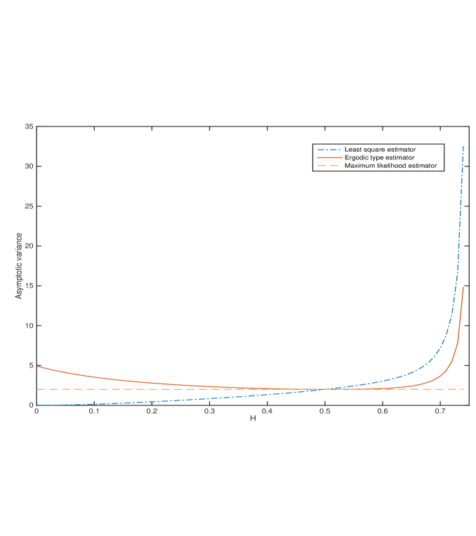
Figure 1: Asymptotic Variance of the Three Estimators

The estimators $\hat{\theta}_{T}$ and $\widetilde{\theta}_{T}$ are based on continuous time data. In practice the process can only be observed at discrete time instants. This motivates us to construct an estimator based on discrete observations. We assume that the fractional Ornstein-Uhlenbeck process $X$ given by (5.2) can be observed at discrete time points $\{t_{k}=kh,k=0,1,\dots,n\}$. We shall use $nh$ instead of $T$ for the time period of the observation. Here $h$ represents the observation frequency and it depends on $n$. We will only consider the high frequency observation case, namely, we shall assume that $h\rightarrow 0$ as $n\rightarrow\infty$. We shall use ergodic type estimator since it can be expressed as a pathwise Riemann integral with respect to time. The following Theorem shows its asymptotic consistency and some results on its asymptotic law.

Theorem 5.6.

Assume the fractional Ornstein-Uhlenbeck process $X$ given by (5.2) is observed at discrete time points $\{t_{k}=kh,k=0,1,...,n\}$. Suppose that $h$ depends on $n$ and as $n\to\infty$, $h$ goes to 0 and $nh$ converges to $\infty$. In addition, we make the following assumptions on $h$ and $n$:

1. When $H\in(0,\frac{3}{4})$, $nh^{p}\rightarrow 0$ for some $p\in(1,\frac{3+2H}{1+2H}\wedge(1+2H))$ as $n\rightarrow\infty$.

2. When $H=\frac{3}{4}$, $\frac{nh^{p}}{\log(nh)}\rightarrow 0$ for some $p\in(1,\frac{9}{5})$ as $n\rightarrow\infty$.

3. When $H\in(\frac{3}{4},1)$, $nh^{p}\rightarrow 0$ for some $p\in(1,\frac{3-H}{2-H})$ as $n\to\infty$.

Set

$$\bar{\theta}_{n}=\left(\frac{1}{n\sigma^{2}H\Gamma(2H)}\sum_{k=1}^{n}X_{kh}^{2}\right)^{-\frac{1}{2H}}\,.$$ (5.22)

Then $\bar{\theta}_{n}$ converges to $\theta$ almost surely as $n\to\infty$. Moreover, as $n$ tends to infinity, we have the following central and noncentral limit theorems.

1. When $H\in(0,\frac{3}{4})$, $\sqrt{nh}(\bar{\theta}_{n}-\theta)\xrightarrow{\mathcal{L}}N(0,\frac{\theta}{(2H)^{2}}\sigma_{H}^{2})$, where $\sigma_{H}^{2}$ is given in Theorem 5.2.

2. When $H=\frac{3}{4}$, $\frac{\sqrt{nh}}{\log(nh)}(\bar{\theta}_{n}-\theta)\xrightarrow{\mathcal{L}}N(0,\frac{16\theta}{9\pi})$.

3. When $H\in(\frac{3}{4},1)$, $(nh)^{2-2H}(\bar{\theta}_{n}-\theta)\xrightarrow{\mathcal{L}}\frac{-\theta^{2H-1}}{H\Gamma(2H+1)}R_{1}$, where $R_{1}=I_{2}(\delta_{0,1})$ is the Rosenblatt random variable and ${\delta}_{0,1}$ is the Dirac-type function defined in (2.6).

Before we prove Theorem 5.6, we state and prove an auxillary result in the following lemma about the regularity of sample paths of the fractional Ornstein-Uhlenbeck process $X$.

Lemma 5.7.

Let $X_{t}$ be given by (5.2). Then for every interval $[0,T]$ and any $0<\epsilon<H$,

$$|X_{t}-X_{s}|\leq V_{1}|t-s|^{H-\epsilon}+V_{2}|t-s|\quad{\rm a.s.},$$ (5.23)

where the random variables $V_{i}$ are defined as follows: $V_{1}=\sigma\eta_{T}$ where $\eta_{T}$ is given by (2.2) with $\alpha=H-\epsilon$, $V_{2}=2\sigma\theta\sup_{u\in[0,T]}|B_{u}^{H}|$.

Proof.

Consider the process $Q_{t}=\sigma\theta\int_{0}^{t}B_{v}^{H}e^{-\theta(t-v)}dv$. Using (5.3), for any $s,t\in[0,T]$ and $s<t$, we have

$$\left|X_{t}-X_{s}\right|=\left|\sigma(B_{t}^{H}-B_{s}^{H})-(Q_{t}-Q_{s})\right|\leq\sigma\left|B_{t}^{H}-B_{s}^{H}\right|+\left|Q_{t}-Q_{s}\right|.$$

Note that

$$|Q_{t}-Q_{s}| \leq \sigma\theta\left|\int_{s}^{t}B_{v}^{H}e^{-\theta(t-v)}dv\right|+\sigma\theta\left|\int_{0}^{s}B_{v}^{H}(e^{-\theta(t-v)}-e^{-\theta(s-v)})dv\right|$$

$$\leq \sigma\theta\sup_{v\in[s,t]}|B_{v}^{H}|\int_{s}^{t}e^{-\theta(t-v)}dv+\sigma\theta\sup_{v\in[s,t]}|B_{v}^{H}|\left(1-e^{-\theta(t-s)}\right)\int_{0}^{s}e^{-\theta(s-v)}dv$$

$$\leq 2\sigma\theta\sup_{v\in[s,t]}|B_{v}^{H}||t-s|\,.$$

Using the above inequality for $|Q_{t}-Q_{s}|$ and Applying (2.2), with $\alpha=H-\epsilon$, for $B_{t}^{H}-B_{s}^{H}$ yield

$$\left|X_{t}-X_{s}\right|\leq\sigma\eta_{T}|t-s|^{H-\epsilon}+2\sigma\theta\sup_{u\in[s,t]}|B_{u}^{H}||t-s|\,.$$

∎

Proof of Theorem 5.6:.

Let $T=nh$, $Z_{n}=\frac{1}{nh}\int^{nh}_{0}X_{t}^{2}dt$, and $\psi_{n}=\frac{1}{n}\sum^{n}_{k=1}X_{kh}^{2}$. Consider the function

$$f(x)=\sqrt{x}\mathbf{1}_{\{0<H<3/4\}}+\sqrt{x}/\log(x)\mathbf{1}_{\{H=3/4\}}+x^{2-2H}\mathbf{1}_{\{3/4<H<1\}}\,.$$

Step 1: We claim that $f(nh)\left|Z_{n}-\psi_{n}\right|\to 0$ almost surely as $n\to\infty$. Applying Markov’s inequality for $\delta>0,q>1$ yields

$$P(f(nh)\left|Z_{n}-\psi_{n}\right|>\delta)\leq\delta^{-q}f(nh)^{q}\mathbb{E}\left|Z_{n}-\psi_{n}\right|^{q}\,.$$ (5.24)

We apply Minkowski’s inequality to obtain

$$\mathbb{E}\left|Z_{n}-\psi_{n}\right|^{q} = (nh)^{-q}\mathbb{E}\Big{|}\sum^{n}_{j=1}\int_{(j-1)h}^{jh}(X_{t}+X_{jh})(X_{t}-X_{jh})dt\Big{|}^{q}$$

$$\leq (nh)^{-q}\left(\sum_{j=1}^{n}\int_{(j-1)h}^{jh}\left(\mathbb{E}(|X_{t}+X_{jh}||X_{t}-X_{jh}|)^{q}\right)^{1/q}dt\right)^{q}\,.$$

Taking into account of Lemma 5.7, we have

$$\mathbb{E}\left|Z_{n}-\psi_{n}\right|^{q}\leq(nh)^{-q}\left(\sum_{j=1}^{n}\int_{(j-1)h}^{jh}\|V_{1}(X_{t}+X_{jh})\|_{L^{q}}|t-jh|^{H-\epsilon}+\|V_{2}(X_{t}+X_{jh})\|_{L^{q}}|t-jh|dt\right)^{q}\,,$$

where the $V_{i}$’s are defined in Lemma 5.7. By Hölder’s inequality and the fact $\|X_{t}\|_{L^{q}}=(\mathbb{E}|X_{t}|^{q})^{1/q}\leq M_{q}$ for all $t>0$, $q>1$, we can write

$$\|V_{i}(X_{t}+X_{jh})\|_{L^{q}}\leq 2M_{qr_{i}}\|V_{i}\|_{qs_{i}}\,,$$

where $1/r_{i}+1/s_{i}=1$. Therefore,

$$\mathbb{E}\left|Z_{n}-\psi_{n}\right|^{q}\leq C\left(M_{qr_{1}}^{q}\|V_{1}\|_{qs_{1}}^{q}h^{q(H-\epsilon)}+M_{qr_{2}}^{q}\|V_{2}\|_{qs_{2}}^{q}h^{q}\right)\,,$$

where $C$ denotes a generic constant.

By (2.2), $\|V_{1}\|_{qs_{1}}^{q}=CT^{q\epsilon}$ for $\epsilon\in(0,H)$. By the self-similarity property of fBm, $\|V_{2}\|_{qs_{2}}^{q}=CT^{qH}$. Using these observations, we obtain

$$\mathbb{E}\left|Z_{n}-\psi_{n}\right|^{q}\leq C\left((nh)^{q\epsilon}h^{q(H-\epsilon)}+(nh)^{qH}h^{q}\right)\,,$$

and plugging this inequality to (5.24), we get

$$P(f(nh)\left|Z_{n}-\psi_{n}\right|>\delta)\leq C\delta^{-q}f(nh)^{q}\left((nh)^{q\epsilon}h^{q(H-\epsilon)}+(nh)^{qH}h^{q}\right)\,.$$ (5.25)

If the right-hand side of the above inequality is summable with respect to $n$, then $f(nh)\left|Z_{n}-\psi_{n}\right|\to 0$ almost surely by the Borel-Cantelli Lemma. We show this summability when $H\in(0,1/2)$ and the other cases are similar. The right-hand side of (5.25) can be written as

$$Cn^{-1-\lambda}\left((nh^{\beta_{1}})^{\gamma_{1}}+(nh^{\beta_{2}})^{\gamma_{2}}\right)\,,$$

where

$$\beta_{1}=\frac{q/2+q\epsilon+q(H-\epsilon)}{1+\lambda+q\epsilon+q/2}\,,\quad\beta_{2}=\frac{3/2q+qH}{1+\lambda+q/2+qH}\,,$$

and $\gamma_{i}$’s are the denominator of $\beta_{i}$’s. Note that the positive variables $\epsilon$ and $\lambda$ can be arbitrarily small and $q$ can be arbitrarily large. In this way, we have $\beta_{1}\in(1,1+2H)$ and $\beta_{2}\in(1,\frac{3+2H}{1+2H})$. If $nh^{p}\to 0$ for some $p\in(1,\min(\frac{3+2H}{1+2H},1+2H))$, then $nh^{\beta_{i}}\to 0$ by carefully choosing these free variables.

Step 2: We prove the almost sure convergence of $\bar{\theta}_{n}$. Denote $\rho=\sigma^{2}H\Gamma(2H)$. Recall that $\widetilde{\theta}_{T}$ is given in Theorem 5.4. By the mean value theorem, we can write

$$\bar{\theta}_{n}-\theta=\left(\frac{\psi_{n}-Z_{n}}{\rho}+\widetilde{\theta}_{T}^{-2H}\right)^{-\frac{1}{2H}}-\theta=\widetilde{\theta}_{T}-\theta+\int_{0}^{1}g_{n}(\lambda)d\lambda,$$ (5.26)

where $g_{n}(\lambda)=-\frac{1}{2H}\frac{\psi_{n}-Z_{n}}{\rho}\left(\lambda\frac{\psi_{n}-Z_{n}}{\rho}+\widetilde{\theta}_{T}^{-2H}\right)^{-\frac{1}{2H}-1}$.

The result in Step 1 also implies $Z_{n}-\psi_{n}\to 0$ almost surely as $n\to\infty$, so $\lim_{n\to\infty}g_{n}(\lambda)=0$ a.s. for all $\lambda\in[0,1]$. Meanwhile, for almost all $\omega$, there exists $N:=N(\omega)\in\mathbb{N}$ such that for $n>N$,

$$\left|\frac{\psi_{n}-Z_{n}}{\rho}\right|<\frac{1}{3}\theta^{-2H},\quad\left|\widetilde{\theta}_{T}^{-2H}-\theta^{-2H}\right|<\frac{1}{3}\theta^{-2H}\,.$$

Then for $n>N$, $|g_{n}(\lambda)|\leq C\theta$. By the dominated convergence theorem,

$$\lim_{n\to\infty}\int_{0}^{1}g_{n}(\lambda)d\lambda=0\quad{\rm a.s.}\,.$$

Then it is clear that $\bar{\theta}_{n}$ converges to $\theta$ almost surely.

Step 3: We prove the asymptotic laws of $\bar{\theta}_{n}$. Equation (5.26) yields

$$f(nh)(\bar{\theta}_{n}-\theta)=f(T)(\widetilde{\theta}_{T}-\theta)+f(nh)\int_{0}^{1}g_{n}(\lambda)d\lambda\,.$$

Using the result of Step 1 and the similar arguments in step 2, we obtain

$$\lim_{n\to\infty}\int_{0}^{1}f(nh)g_{n}(\lambda)d\lambda=0\quad{\rm a.s.}\,.$$

Then it is clear that $f(nh)(\bar{\theta}_{n}-\theta)$ converges in law to the same random variable as $f(T)(\widetilde{\theta}_{T}-\theta)$ when $T$ tends to infinity. By Theorem 5.4, we finish the proof.

∎

6 Appendix

This section contains some technical results needed in the proofs of the main theorems of the paper. First we need to identify the limits of some multiple integrals. Denote

$$\psi(x,u)=\psi_{T}(x,u)=T^{4H+1}e^{-\theta T(u+x)}\;,$$ (6.1)

$$\varphi_{1}(x) := \int^{1}_{x}[(t-x)^{2H-1}-1][(1-t)^{2H-1}-(1-t+x)^{2H-1}]dt\,,$$ (6.2)

$$\varphi_{2}(x) := \int^{1}_{x}[(t-x)^{2H-1}-t^{2H-1}](1-t+x)^{2H-1}dt\,,$$ (6.3)

$$\varphi_{3}(x,u) := \int^{1}_{x}[{\rm sgn}(u-t)|u-t|^{2H-1}-{\rm sgn}(x+u-t)|x+u-t|^{2H-1}]dt\,,$$ (6.4)

$$\varphi_{4}(x,u) := \int^{1}_{x}t^{2H-1}{\rm sgn}(x+u-t)|x+u-t|^{2H-1}$$ (6.5)

$$-(t-x)^{2H-1}{\rm sgn}(u-t)|u-t|^{2H-1}dt\,,$$

$$\varphi_{5}(x,u) := \int_{x}^{1}{\rm sgn}(x+u-t)|x+u-t|^{2H-1}(1-t)^{2H-1}$$ (6.6)

$$-{\rm sgn}(u-t)|u-t|^{2H-1}(1-t+x)^{2H-1}dt\,.$$

Fix an $\epsilon\in(0,\frac{1}{4})$. Denote $[0,1]^{2}=\mathcal{I}_{1}\cup\mathcal{I}_{2}$ where $\mathcal{I}_{1}=[0,\epsilon]^{2}$ and $\mathcal{I}_{2}=[0,1]^{2}\backslash[0,\epsilon]^{2}$.

Lemma 6.1.

Let $H\in(0,\frac{1}{2})$. When $x,u\in\mathcal{I}_{1}$, we have the following estimates.

1. $$|\varphi_{1}(x)|\leq x^{2H}\,,$$ (6.7)

2. $$|\varphi_{3}(x,u)|\leq C(x^{2H}+u^{2H}+|u-x|^{2H})\,,$$ (6.8)

3. $$|\varphi_{5}(x,u)|\leq C(x^{2H}+u^{2H}+|u-x|^{2H})\,,$$ (6.9)

where $C$ is a constant independent of $x,u$.

Proof.

First we prove (6.7). Observe that

$$0\leq\varphi_{1}(x)\leq\int_{x}^{1}f(x,t)dt,$$ (6.10)

where

$$f(x,t)=(t-x)^{2H-1}[(1-t)^{2H-1}-(1-t+x)^{2H-1}]\,.$$

It is clear that for $\frac{1+x}{2}\leq t\leq 1$

$$f(x,t)\leq\big{(}\frac{1-x}{2}\big{)}^{2H-1}[(1-t)^{2H-1}-(1-t+x)^{2H-1}]\,,$$

whereas for $x\leq t\leq\frac{1+x}{2}$. Applying the mean value theorem for the second factor of $f(x,t)$ yields

$$f(x,t)\leq(1-2H)(t-x)^{2H-1}\big{(}\frac{1-x}{2}\big{)}^{2H-2}x\,.$$

Integrating the right-hand side of the above two inequalities with respect to $t$, we obtain

$$\int_{x}^{1}f(x,t)dt \leq \frac{1}{2H}\big{(}\frac{1-x}{2}\big{)}^{2H-1}\big{[}\big{(}\frac{1-x}{2}\big{)}^{2H}-\big{(}\frac{1+x}{2}\big{)}^{2H}+x^{2H}\big{]}+\frac{1-2H}{2H}\big{(}\frac{1-x}{2}\big{)}^{4H-2}x$$

$$\leq \frac{1}{2H}\big{(}\frac{1-\epsilon}{2}\big{)}^{2H-1}x^{2H}+\frac{1-2H}{2H}\big{(}\frac{1-\epsilon}{2}\big{)}^{4H-2}x^{2H}\;,$$

where we have used the inequality $x<x^{2H}$ on $\mathcal{I}_{1}$ (i.e., $x\in(0,\epsilon)$). Thus, (6.7) follows from the above inequality and (6.10).

Next we prove (6.8). Note that the antiderivative of the function ${\rm sgn}(x)|x|^{2H-1}$ is $(2H)^{-1}|x|^{2H}$, so we can compute $\varphi_{3}(x,u)$ as follows

$$\varphi_{3}(x,u)=\frac{1}{2H}(|u-x|^{2H}-(1-u)^{2H}+(1-x-u)^{2H}-u^{2H})\,.\\$$ (6.11)

Applying the inequality

$$\left|(1-x-u)^{2H}-(1-u)^{2H}\right|\leq 2H(1-x-u)^{2H-1}x\leq 2H(1-2\epsilon)^{2H-1}x^{2H}\;,$$

and the triangular inequality to (6.11) yields

$$|\varphi_{3}(x,u)| \leq (2H)^{-1}(|u-x|^{2H}+u^{2H}+2H(1-2\epsilon)^{2H-1}x^{2H})$$

$$\leq C(|u-x|^{2H}+u^{2H}+x^{2H})\quad\forall\;x,u\in\mathcal{I}_{1}\,.$$

Finally, we prove (6.9). Denote

$$\zeta_{x,u}(t)={\rm sgn}(x+u-t)|x+u-t|^{2H-1}(1-t)^{2H-1}-{\rm sgn}(u-t)|u-t|^{2H-1}(1-t+x)^{2H-1}.$$

Let $\delta\in(\frac{1}{2},1)$. Since $\epsilon\in(0,\frac{1}{4})$ and $(x,u)\in(0,\epsilon)^{2}$, the interval $(x,1)$ can be decomposed into the following three intervals, where

$$J_{1}=(x,\,u+x),\quad J_{2}=(u+x,\,\delta),\quad J_{3}=(\delta,\,1)\,.$$

Then $\varphi_{5}(x,u)=\sum_{k=1}^{3}\int_{J_{k}}\zeta_{x,u}(t)dt$. We consider the above three integrals separately.

Case 1: When $t\in J_{1}$, we have

$$(1-t)^{2H-1}\leq(1-u-x)^{2H-1}\leq(1-2\epsilon)^{2H-1}\,.$$ (6.12)

When $t$ falls in different subintervals of $J_{1}$, we bound $(1-t+x)^{2H-1}$ in different ways. Namely, if $t\in(x,u)$ and $u\geq x$,

$$(1-t+x)^{2H-1}\leq(1+x-u)^{2H-1}\leq(1-\epsilon)^{2H-1}\,.$$ (6.13)

If $t\in(x\vee u,x+u)$,

$$(1-t+x)^{2H-1}\leq(1-u)^{2H-1}\leq(1-\epsilon)^{2H-1}\,.$$ (6.14)

Applying (6.12) for the first summand in $\zeta_{x,u}(t)$, (6.13) and (6.14) for the second summand, we can bound the integration of $\zeta_{x,u}(t)$ on $J_{1}$ as follows

$$\Big{|}\int_{J_{1}}\zeta_{x,u}(t)dt\Big{|} \leq (1-2\epsilon)^{2H-1}\int_{x}^{u+x}(x+u-t)^{2H-1}dt$$

$$+\,(1-\epsilon)^{2H-1}\big{(}\int_{x}^{u}(u-t)^{2H-1}1_{\{u\geq x\}}dt+\int_{x\vee u}^{x+u}(t-u)^{2H-1}dt\big{)}\,.$$

Integrating with respect to $t$ yields

$$\Big{|}\int_{J_{1}}\zeta_{x,u}(t)dt\Big{|}\leq C(u^{2H}+(u-x)^{2H}1_{\{u\geq x\}}+x^{2H})\,.$$

Case 2: For $t\in J_{2}$, we rewrite

$$-\int_{J_{2}}\zeta_{x,u}(t)dt = \int_{u+x}^{\delta}(1-t)^{2H-1}\big{(}(t-u-x)^{2H-1}-(t-u)^{2H-1}\big{)}$$

$$+\;(t-u)^{2H-1}\big{(}(1-t)^{2H-1}-(1-t+x)^{2H-1}\big{)}dt\,,$$

which is nonnegative. In the above integrand, we bound $(1-t)^{2H-1}$ by $(1-\delta)^{2H-1}$ for the first summand. For the second summand, we apply the mean value theorem for the difference part and bound $(t-u)^{2H-1}$ by $x^{2H-1}$. Then integrating $t$ yields

$$0\leq-\int_{J_{2}}\zeta_{x,u}(t)dt \leq \frac{(1-\delta)^{2H-1}}{2H}\big{(}(\delta-u-x)^{2H}-(\delta-u)^{2H}+x^{2H}\big{)}$$

$$+\;x^{2H}\big{(}(1-\delta)^{2H-1}-(1-u-x)^{2H-1}\big{)}$$

$$\leq \frac{(1-\delta)^{2H-1}}{2H}x^{2H}+(1-\delta)^{2H-1}x^{2H}\leq Cx^{2H}\;.$$

Case 3: For $t\in J_{3}$, we rewrite

$$-\int_{J_{3}}\zeta_{x,u}(t)dt = \int_{\delta}^{1}(t-u-x)^{2H-1}((1-t)^{2H-1}-(1-t+x)^{2H-1})$$

$$+\;(1-t+x)^{2H-1}((t-u-x)^{2H-1}-(t-u)^{2H-1})dt\,,$$

which is nonnegative. In the above integrand, we bound $(t-u-x)^{2H-1}$ by $(\delta-2\epsilon)^{2H-1}$ for the first summand. For the second summand, apply the mean value theorem for the difference part and bound $(1-t+x)^{2H-1}$ by $x^{2H-1}$. Then integrating $t$ yields

$$0\leq-\int_{J_{3}}\zeta_{x,u}(t)dt \leq \frac{(\delta-2\epsilon)^{2H-1}}{2H}\big{(}(1-\delta)^{2H}-(1-\delta+x)^{2H}+x^{2H}\big{)}$$

$$+\;x^{2H}\big{(}(\delta-u-x)^{2H-1}-(1-u-x)^{2H-1}\big{)}$$

$$\leq \frac{(\delta-2\epsilon)^{2H-1}}{2H}x^{2H}+x^{2H}(\delta-u-x)^{2H-1}\leq Cx^{2H}\,.$$

In the last step we have applied the inequality $\delta-u-x\geq\delta-2\epsilon$. ∎

Lemma 6.2.

Suppose $H\in(0,\frac{1}{2})$. Let $\psi(x,u)$ and $\varphi_{4}(x,u)$ defined by (6.1) and (6.5), respectively. Fix $\epsilon\in(0,1/4)$. Then

$$\lim_{T\to\infty}\int_{[0,\epsilon]^{2}}\psi(x,u)(x^{2H}+u^{2H}+|x-u|^{2H})=0\,,$$ (6.15)

and

$$\lim_{T\to\infty}\int_{[0,1]^{2}}\psi(x,u)\varphi_{4}(x,u)dxdu$$

$$\qquad=\theta^{-1-4H}\Big{(}\Gamma(2H)^{2}(2H-2^{-1})+\frac{\Gamma(2-4H)\Gamma(2H)\Gamma(4H)}{\Gamma(1-2H)}\Big{)}\,.$$ (6.16)

Proof.

We first prove (6.15). For the first summand, making the change of variables $Tx\to x_{1}$ and $Tu\to x_{2}$ yields

$$\int_{[0,\epsilon]^{2}}T^{4H+1}e^{-\theta T(x+u)}x^{2H}dxdu=T^{2H-1}\int_{[0,T\epsilon]^{2}}e^{-\theta(x_{1}+x_{2})}x_{1}^{2H}dx_{1}dx_{2}\;,$$ (6.17)

which goes to $0$ as $T\to\infty$. A similar argument could be applied to the second summand. For the third summand, by symmetry it suffices to consider the integral on the region $\{u>x\}$. Making the change of variables $T(u-x)\to x_{1}$, $Tx\to x_{2}$ yields

$$\int_{[0,\epsilon]^{2}}T^{4H+1}e^{-\theta T(x+u)}|u-x|^{2H}dxdu=2T^{2H-1}\int_{[0,T\epsilon]^{2},x_{1}+x_{2}\leq T\epsilon}e^{-\theta(x_{1}+2x_{2})}x_{1}^{2H}dx_{1}dx_{2}\;,$$ (6.18)

which goes to $0$ as $T\to\infty$.

Next we show (6.16). Set

$$\Theta:=\lim_{T\rightarrow\infty}\int_{[0,1]^{2}}\psi(x,u)\varphi_{4}(x,u)dxdu.$$

Making change of variables, $\theta Tx\to x,\theta Tu\to u,\theta Tt\to t$, we can write

$$\Theta = \theta^{-1-4H}\int_{[0,\infty)^{2}}e^{-(u+x)}dxdu$$

$$\times\int^{\infty}_{x}[t^{2H-1}{\rm sgn}(x+u-t)|x+u-t|^{2H-1}-(t-x)^{2H-1}{\rm sgn}(u-t)|u-t|^{2H-1}]dt\,.$$

The above integral can be decomposed as follows

$$\Theta=\theta^{-1-4H}(L_{1}-L_{2}+L_{3})\;,$$

where

$$L_{1}:=\int_{[0,\infty)^{2}}e^{-(x+u)}dxdu\int_{x}^{x+u}t^{2H-1}(x+u-t)^{2H-1}dt\;,$$

$$L_{2}:=\int_{[0,\infty)^{2},u>x}e^{-(x+u)}dxdu\int_{x}^{u}(t-x)^{2H-1}(u-t)^{2H-1}dt\;,$$

$$L_{3}:=\int_{[0,\infty)^{2}}e^{-(x+u)}dxdu\Big{(}\int_{u\vee x}^{\infty}(t-x)^{2H-1}(t-u)^{2H-1}dt-\int_{x+u}^{\infty}t^{2H-1}(t-x-u)^{2H-1}dt\Big{)}\,.$$

Making the change of variables $t-x\to s$ and integrating $u$, we obtain

$$L_{1}=\Gamma(2H)\int_{[0,\infty)^{2}}e^{-(x+s)}(x+s)^{2H-1}dxds=\Gamma(2H)^{2}2H\,.$$

Denote by ${\rm B}(\alpha,\beta)$ the Beta function. Then

$$L_{2}={\rm B}(2H,2H)\int_{[0,\infty)^{2},u>x}e^{-(x+u)}(u-x)^{4H-1}dxdu\,.$$

By setting $u-x\to v$ and integrating in $x$ first, we deduce $L_{2}=\Gamma(2H)^{2}/2$. To compute $L_{3}$, by symmetry it suffices to integrate on the region $\{u<x\}$. For the second integral, we make the change of variables $t-u\to y$. In this way, we obtain

$$L_{3}=2\int_{0<u<x<y<\infty}e^{-(u+x)}((y-u)^{2H-1}-(y+u)^{2H-1})(y-x)^{2H-1}dydxdu.$$

The change of variables $x-u\to a,y-x\to b$ yields

$$L_{3} = 2\int_{\mathbb{R}_{+}^{3}}e^{-(a+2u)}b^{2H-1}\big{[}(a+b)^{2H-1}-(a+b+2u)^{2H-1}\big{]}dudadb$$

$$= 2\int_{\mathbb{R}_{+}^{3}}e^{-(a+2u)}b^{2H-1}dudadb\int_{a}^{2u+a}(1-2H)(b+z)^{2H-2}dz$$

$$= 2(1-2H)\int_{\mathbb{R}_{+}^{2}}e^{-(a+2u)}duda\int_{a}^{2u+a}(\int_{\mathbb{R}_{+}}b^{2H-1}(b+z)^{2H-2}db)dz\,.$$

Setting $z/(b+z)\to v$ and integrating $v$ on $[0,1]$, we obtain

$$L_{3} = 2(1-2H){\rm B}(2-4H,2H)\int_{\mathbb{R}_{+}^{2}}e^{-(a+2u)}duda\int_{a}^{2u+a}z^{4H-2}dz$$

$$= \frac{\Gamma(2-4H)\Gamma(2H)\Gamma(4H)}{\Gamma(1-2H)}\,.$$

Then, the lemma follows from the above computations of $L_{1}$, $L_{2}$ and $L_{3}$. ∎

Lemma 6.3.

Denote $\mathcal{I}_{1}=[0,\epsilon]^{2}$ and $\mathcal{I}_{2}=[0,1]^{2}\backslash[0,\epsilon]^{2}$. The functions $\psi$ and $\varphi_{i}$ are given by (6.1) to (6.6). For $j=1,2$ and $i=1,2,3,5$, we have the following result.

$$\lim_{T\rightarrow\infty}\int_{\mathcal{I}_{j}}\psi\varphi_{i}dxdu=0\,.$$ (6.19)

Proof.

The proof of (6.19) is divided into the cases $j=2$ and $j=1$.

Case $j=2$: Clearly, for $(x,u)\in\mathcal{I}_{2}$,

$$\psi(x,u)\leq T^{4H+1}e^{-\theta T\epsilon},$$ (6.20)

which implies

$$\int_{\mathcal{I}_{2}}\psi\varphi_{i}dxdu\;\to 0{\text{\quad for}\;}i=1,2,3,5$$ (6.21)

as $T\to\infty$. Thus, (6.19) holds true for $j=2$.

Case $j=1$: For $i=2$, we evaluate the integral of $\psi\varphi_{2}$ on $\mathcal{I}_{1}$ by making change of variables $Tx\to x$, $Tu\to u$ and $Tt\to t$. In this way, we obtain

$$\int_{\mathcal{I}_{1}}\psi\varphi_{2}dxdu=\int_{[0,T\epsilon]^{2}}e^{-\theta(u+x)}dxdu\int^{T}_{x}[(t-x)^{2H-1}-t^{2H-1}](T-t+x)^{2H-1}dt\,.$$ (6.22)

Clearly $(T-t+x)^{2H-1}\leq x^{2H-1}$, so the integrand of the above triple integral is bounded by the function $e^{-\theta(u+x)}((t-x)^{2H-1}-t^{2H-1})\mathbf{1}_{\{t\geq x\}}x^{2H-1}$ which is integrable on $[0,\infty)^{3}$. As $T\to\infty$, $(T-t+x)^{2H-1}\to 0$. Applying the dominated convergence theorem, we have

$$\lim_{T\to\infty}\int_{\mathcal{I}_{1}}\psi\varphi_{2}dxdu=0.$$ (6.23)

The cases $i=1,3,5$ follows from (6.7), (6.8) and (6.9) and Lemma 6.2. ∎

Lemma 6.4.

Let $H\in(0,\frac{1}{2})$. Denote $f_{\alpha}(\xi,\eta,\eta^{\prime})=|\xi-\eta|^{-1+\alpha}|\xi-\eta^{\prime}|^{-1+\alpha}\xi^{1-2H}$ where $\xi,\eta,\eta^{\prime}\in\mathbb{R}_{+}$. Assuming $\eta\geq\eta^{\prime}$ and $0<\alpha<\frac{1}{2}$, we have the following results.

(i)

For any $0<\epsilon<\alpha$, there exists some positive constants $K_{1},K_{2}$ depending on $\alpha,\epsilon$ such that

$$\int_{(0,\eta+\eta^{\prime})}f_{\alpha}(\xi,\eta,\eta^{\prime})d\xi\leq K_{1}(\eta-\eta^{\prime})^{-1+2\alpha-\epsilon}\eta^{1-2H+\epsilon}+K_{2}(\eta-\eta^{\prime})^{-1+2\alpha}\eta^{1-2H}\,.$$

(ii)

If $\alpha\in(0,H)$, then there exists some positive constants $K_{3},K_{4}$ depending on $\alpha$ and $H$ such that

$$\int_{[\eta+\eta^{\prime},\infty)}f_{\alpha}(\xi,\eta,\eta^{\prime})d\xi\leq K_{3}(\eta^{\prime})^{2\alpha-2H}+K_{4}\eta^{1-2H}(\eta^{\prime})^{-1+2\alpha}\,.$$

Proof.

We partition $(0,\eta+\eta^{\prime})$ into three intervals: $(0,\eta^{\prime}]\cup(\eta^{\prime},\eta]\cup(\eta,\eta+\eta^{\prime})$. We shall use the inequality

$$(a+b)^{-r}\leq a^{-s}b^{-r+s},\quad\hbox{ for any}\ 0<s<r{\rm\;and\;}a,b\in\mathbb{R}_{+}.$$ (6.24)

For any $0<\epsilon<\alpha$, we write $\xi-\eta^{\prime}=(\eta-\eta^{\prime})+(\xi-\eta)$ and apply (6.24) for $(\xi-\eta^{\prime})^{-1+\alpha}$ with $s=1-2\alpha+\epsilon$. In this way, we obtain

$$\int_{\eta}^{\eta+\eta^{\prime}}f_{\alpha}(\xi,\eta,\eta^{\prime})d\xi \leq \int_{\eta}^{\eta+\eta^{\prime}}(\xi-\eta)^{-1+\alpha}(\eta-\eta^{\prime})^{-(1-2\alpha+\epsilon)}(\xi-\eta)^{(-1+\alpha)+(1-2\alpha+\epsilon)}\xi^{1-2H}d\xi$$ (6.25)

$$\leq (\eta-\eta^{\prime})^{-1+2\alpha-\epsilon}(\eta+\eta^{\prime})^{1-2H}\int_{\eta}^{\eta+\eta^{\prime}}(\xi-\eta)^{-1+\epsilon}d\xi$$

$$\leq 2^{1-2H}\epsilon^{-1}(\eta-\eta^{\prime})^{-1+2\alpha-\epsilon}\eta^{1-2H+\epsilon}\;.$$

For $\xi\in(\eta^{\prime},\eta]$, observe that

$$\int_{\eta^{\prime}}^{\eta}f_{\alpha}(\xi,\eta,\eta^{\prime})d\xi \leq \eta^{1-2H}\int_{\eta^{\prime}}^{\eta}(\eta-\xi)^{-1+\alpha}(\xi-\eta^{\prime})^{-1+\alpha}d\xi$$ (6.26)

$$\leq \eta^{1-2H}\int_{0}^{\eta-\eta^{\prime}}(\eta-\eta^{\prime}-\xi)^{-1+\alpha}\xi^{-1+\alpha}d\xi$$

$$\leq K_{2}\eta^{1-2H}(\eta-\eta^{\prime})^{-1+2\alpha},$$

where $K_{2}={\rm B}(\alpha,\alpha)$. For $\xi\in(0,\eta^{\prime}]$, writing $\eta-\xi=(\eta-\eta^{\prime})+(\eta^{\prime}-\xi)$ and applying (6.24) with $s=1-2\alpha+\epsilon$ again (for the same $\epsilon$ as above), we obtain

$$\int_{0}^{\eta^{\prime}}f_{\alpha}(\xi,\eta,\eta^{\prime})d\xi \leq (\eta^{\prime})^{1-2H}\int_{0}^{\eta^{\prime}}(\eta-\xi)^{-1+\alpha}(\eta^{\prime}-\xi)^{-1+\alpha}d\xi$$

$$\leq (\eta^{\prime})^{1-2H}\int_{0}^{\eta^{\prime}}(\eta-\eta^{\prime})^{-(1-2\alpha+\epsilon)}(\eta^{\prime}-\xi)^{(-1+\alpha)+(1-2\alpha+\epsilon)}(\eta^{\prime}-\xi)^{-1+\alpha}d\xi$$

$$\leq \epsilon^{-1}\eta^{1-2H+\epsilon}(\eta-\eta^{\prime})^{-1+2\alpha-\epsilon}.$$ (6.28)

Let $K_{1}=3\epsilon^{-1}$. By (6.25), (6.26), and (6.28), the first part of lemma is obtained.

Now if $\alpha\in(0,H)$, then

$$\int_{\eta+\eta^{\prime}}^{\infty}f_{\alpha}(\xi,\eta,\eta^{\prime})d\xi \leq \int_{\eta+\eta^{\prime}}^{\infty}(\xi-\eta)^{-2+2\alpha}\xi^{1-2H}d\xi=\int_{\eta^{\prime}}^{\infty}\xi^{-2+2\alpha}(\xi+\eta)^{1-2H}d\xi$$ (6.29)

$$\leq\int_{\eta^{\prime}}^{\infty}\xi^{-2+2\alpha}(\xi^{1-2H}+\eta^{1-2H})d\xi$$

$$=K_{3}(\eta^{\prime})^{2\alpha-2H}+K_{4}\eta^{1-2H}(\eta^{\prime})^{-1+2\alpha},$$

where in the third step, we apply the inequality $(\xi+\eta)^{1-2H}\leq\xi^{1-2H}+\eta^{1-2H}$ for $H\in(0,\frac{1}{2})$. Here the constants $K_{3}=(2H-2\alpha)^{-1}$, $K_{4}=(1-2\alpha)^{-1}$. This finishes the proof of the lemma.
∎

Lemma 6.5.

For $n\geq 0$, and $H\in[\frac{3}{4},1)$, set

$$A_{1,H}(T)={T^{3-4H}}\int^{T}_{0}\int^{T-t}_{0}s^{n}e^{-\theta s}t^{2H-2}(s+t)^{2H-2}dsdt,$$

and

$$A_{2,H}(T)=T^{3-4H}\int^{T}_{0}\int^{T}_{0}s^{n}e^{-\theta s}t^{2H-2}(s+t)^{2H-2}dsdt.$$

Then

1. For $H\in(\frac{3}{4},1)$, $\displaystyle\lim_{T\to\infty}A_{1,H}(T)=\displaystyle\lim_{T\to\infty}A_{2,H}(T)=\frac{\theta^{-(n+1)}\Gamma(n+1)}{4H-3}$;
   

2. For $H=\frac{3}{4}$, $\displaystyle\lim_{T\to\infty}\frac{A_{1,H}(T)}{\log T}=\displaystyle\lim_{T\to\infty}\frac{A_{2,H}(T)}{\log T}=\Gamma(n+1)\theta^{-(n+1)}$.
   

Proof.

(i) For $H\in(\frac{3}{4},1)$, we have

$$A_{2,H}(T)\leq T^{3-4H}\int^{T}_{0}\int^{T}_{0}s^{n}e^{-\theta s}t^{4H-4}dsdt,$$

and

$$A_{1,H}(T)\geq T^{3-4H}\int^{T}_{0}\int^{T-t}_{0}s^{n}e^{-\theta s}(s+t)^{4H-4}dsdt.$$

For the right-hand sides of the above two inequalities, we integrate first in $t$ to obtain

$$\frac{1}{4H-3}\left(\int_{0}^{T}s^{n}e^{-\theta s}ds-T^{3-4H}\int_{0}^{T}s^{n+4H-3}e^{-\theta s}ds\right)$$

$$\qquad\qquad\leq A_{1,H}(T)\leq A_{2,H}(T)\leq\frac{1}{4H-3}\int^{T}_{0}s^{n}e^{-\theta s}ds.$$

This yields (i) by letting $T\to\infty$.

(ii) For $H=\frac{3}{4}$, by the L’Hopital rule, we have

$$\lim_{T\to\infty}\frac{A_{2,H}(T)}{\log T}=\lim_{T\to\infty}T\Big{[}\int^{T}_{0}s^{n}e^{-\theta s}T^{-\frac{1}{2}}(s+T)^{-\frac{1}{2}}ds+\int^{T}_{0}T^{n}e^{-\theta T}t^{-\frac{1}{2}}(T+t)^{-\frac{1}{2}}dt\Big{]}.$$

The second summand on the right-hand side of the above equation goes to 0 as $T\to\infty$, so

$$\lim_{T\to\infty}\frac{A_{2,H}(T)}{\log T}\leq\int^{\infty}_{0}s^{n}e^{-\theta s}ds.$$ (6.30)

On the other hand, by the inequality $t\leq s+t$,

$$\frac{A_{1,H}(T)}{\log T} \geq \frac{1}{\log T}\displaystyle\int^{T}_{0}\int^{T-t}_{0}s^{n}e^{-\theta s}(s+t)^{-1}dsdt$$

$$= \frac{1}{\log T}\Big{[}\log T\int^{T}_{0}s^{n}e^{-\theta s}ds-\int^{T}_{0}s^{n}e^{-\theta s}\log sds\Big{]}.$$

The function $s^{n}e^{-\theta s}\log s$ is integrable on $[0,\infty)$. Thus,

$$\lim_{T\to\infty}\frac{A_{1,H}(T)}{\log T}\geq\int^{\infty}_{0}s^{n}e^{-\theta s}ds.$$ (6.31)

By (6.30) and (6.31), we conclude the proof of (ii). ∎

Lemma 6.6.

Let $F_{T}$, $\widetilde{F}_{T}$ be defined by (5.11) and (5.19), respectively. Moreover, let $R_{1}$ be defined in Part (iii) of Theorem 5.2. Then we have the following convergence results.

(i)

When $0<H<\frac{1}{2}$ we have

$$\lim_{T\to\infty}\mathbb{E}\left(\frac{1}{T}F_{T}^{2}\right)=4H^{2}\theta^{1-4H}\Gamma(2H)^{2}\Big{(}(4H-1)+\frac{2\Gamma(2-4H)\Gamma(4H)}{\Gamma(2H)\Gamma(1-2H)}\Big{)}\,.$$ (6.32)

(ii)

When $H=\frac{3}{4}$, we have

$$\lim_{T\to\infty}\frac{\mathbb{E}\left(F_{T}^{2}\right)}{T\log(T)}=9/4\theta^{-2}\,\,.$$ (6.33)

(iii)

When $H>\frac{3}{4}$, we have

$$\lim_{T\to\infty}\mathbb{E}\left(T^{2-4H}F_{T}^{2}\right)=\frac{16\alpha_{H}^{2}\theta^{-2}}{(4H-2)(4H-3)}\,,$$ (6.34)

$$\lim_{T\to\infty}\mathbb{E}[T^{1-2H}R_{1}\widetilde{F}_{T}]=\frac{8\alpha_{H}^{2}\theta^{-1}}{(4H-2)(4H-3)}\,,$$ (6.35)

where $\alpha_{H}=H(2H-1)$.

In the above lemma, we do not give a statement when $H\in[\frac{1}{2},\frac{3}{4})$, because this case has been studied in [11].

Proof.

Part (i): Assume $H\in(0,\frac{1}{2})$. Applying L’Hopital’s rule to (5.12) yields

$$\lim_{T\to\infty}\mathbb{E}\left(\frac{1}{T}F_{T}^{2}\right)=\lim_{T\to\infty}4H^{2}\theta^{2}(I_{1}+I_{2})\,,$$ (6.36)

where

$$I_{1}=(H\theta)^{-1}\int_{[0,T]^{3}}e^{-\theta(T-t_{1})}\frac{\partial e^{-\theta|s_{2}-t_{2}|}}{\partial s_{2}}[T^{2H-1}-(T-s_{2})^{2H-1}]\frac{\partial R_{H}(t_{1},t_{2})}{\partial t_{2}}ds_{2}dt_{1}dt_{2}\,,$$

$$I_{2}=-(H\theta)^{-1}\int_{[0,T]^{3}}e^{-\theta(T-s_{1})}\frac{\partial e^{-\theta|s_{2}-t_{2}|}}{\partial s_{2}}\frac{\partial R_{H}(s_{1},s_{2})}{\partial s_{1}}$$

$$\qquad\qquad\times[t_{2}^{2H-1}+(T-t_{2})^{2H-1}]ds_{1}ds_{2}dt_{2}\,.$$ (6.37)

To compute the limit of $\mathbb{E}(\frac{1}{T}F_{T}^{2})$ we will consider that of $I_{1}$ and $I_{2}$.

Computation of $\lim_{T\to\infty}I_{1}$:  We first compute explicitly the partial derivatives in the integrand of $I_{1}$. On the region $\{t_{2}>s_{2}\}$, we make change of variables $1-\frac{t_{1}}{T}\to u$, $\frac{t_{2}}{T}-\frac{s_{2}}{T}\to x$ and $1-\frac{s_{2}}{T}\to t$, and on the region $\{t_{2}<s_{2}\}$, we make change of variables $1-\frac{t_{1}}{T}\to u$, $\frac{s_{2}}{T}-\frac{t_{2}}{T}\to x$ and $1-\frac{t_{2}}{T}\to t$. In this way, $I_{1}$ can be written as

$$I_{1} = \int_{[0,1]^{3},x\leq t}T^{4H+1}e^{-\theta T(u+x)}(1-t^{2H-1})$$

$$\qquad\left((1-t+x)^{2H-1}-{\rm sgn}(x+u-t)|x+u-t|^{2H-1}\right)dudxdt$$

$$-\int_{[0,1]^{3},x\leq t}T^{4H+1}e^{-\theta T(u+x)}\left(1-(t-x)^{2H-1}\right)\left((1-t)^{2H-1}-{\rm sgn}(u-t)|u-t|^{2H-1}\right)dudxdt\,.$$

Reorganize the terms in the above integrals we have

$$I_{1}=\int_{[0,1]^{2}}\psi(x,u)\sum_{i=1}^{4}\varphi_{i}dxdu\,,$$ (6.39)

where the functions $\psi$, $\varphi_{i}$ are given by (6.1) to (6.5).

By (6.19), we see

$$\lim_{T\to\infty}I_{1}=\lim_{T\to\infty}\int_{[0,1]^{2}}\psi(x,u)\varphi_{4}(x,u)dxdu\,,$$ (6.40)

whose value is computed in (6.16) of Lemma 6.2.

Computation of $\lim_{T\to\infty}I_{2}$: We first compute explicitly the partial derivatives in the integrand of (6.37). On the region $\{s_{2}>t_{2}\}$, we make change of variables $T-s_{1}\to Tu$, $s_{2}-t_{2}\to Tx$ and $T-t_{2}\to Tt$, and on the region $\{t_{2}>s_{2}\}$, we make change of variables $T-s_{1}\to Tu$, $t_{2}-s_{2}\to Tx$ and $T-s_{2}\to Tt$. In this way,

$$I_{2} = \int_{[0,1]^{3},t\geq x}T^{4H+1}e^{-\theta T(u+x)}\left((1-u)^{2H-1}+{\rm sgn}(x+u-t)|x+u-t|^{2H-1}\right)$$

$$\left(t^{2H-1}+(1-t)^{2H-1}\right)dudxdt-\int_{[0,1]^{3},t\geq x}T^{4H+1}e^{-\theta T(u+x)}$$

$$\left((1-u)^{2H-1}+{\rm sgn}(u-t)|u-t|^{2H-1}\right)\left((1-t+x)^{2H-1}+(t-x)^{2H-1}\right)dudxdt\,.$$

Note that

$$\int_{x}^{1}\left(t^{2H-1}+(1-t)^{2H-1}\right)-\left((1-t+x)^{2H-1}+(t-x)^{2H-1}\right)dt=0\;,$$

so $I_{2}$ can be simplified and rewritten as

$$I_{2}=\int_{[0,1]^{2}}\psi(x,u)\big{(}\varphi_{4}(x,u)+\varphi_{5}(x,u)\big{)}dxdu\;,$$ (6.42)

where $\psi(x,u)$, $\varphi_{4}(x,u)$ and $\varphi_{5}(x,u)$ are given by (6.1), (6.5) and (6.6) respectively. By (6.40) and the result of (6.19) for $i=5$, we have

$$\lim_{T\to\infty}I_{2}=\lim_{T\to\infty}I_{1}\,.$$ (6.43)

Then part (i) follows from (6.36), (6.40), (6.43) and (6.16).

Part (ii) and (iii): Assume $H\geq 3/4$. Using (2.5), we have

$$\mathbb{E}(F_{T}^{2})=2\alpha_{H}^{2}I_{T}\,,$$ (6.44)

where $\alpha_{H}=H(2H-1)$, and

$$I_{T}=\int_{[0,T]^{4}}e^{-\theta|s_{2}-u_{2}|-\theta|s_{1}-u_{1}|}|s_{2}-s_{1}|^{2H-2}|u_{2}-u_{1}|^{2H-2}du_{1}du_{2}ds_{1}ds_{2}\,.$$ (6.45)

Applying L’Hopital rule yields

$$\lim_{T\to\infty}\mathbb{E}(T^{2-4H}F_{T}^{2})=\frac{8\alpha_{H}^{2}}{4H-2}\lim_{T\to\infty}T^{3-4H}J_{T} H\in(\frac{3}{4},1)$$ when (6.46)

$$\lim_{T\to\infty}\frac{\mathbb{E}F_{T}^{2}}{T\log T}=\frac{9}{8}\lim_{T\to\infty}\frac{J_{T}}{\log T} \qquad\hbox{when $H=\frac{3}{4}$},$$ (6.47)

where

$$J_{T}=\int_{[0,T]^{3}}e^{-\theta|T-u_{2}|-\theta|s_{1}-u_{1}|}(T-s_{1})^{2H-2}|u_{2}-u_{1}|^{2H-2}du_{1}du_{2}ds_{1}\,.$$

Denote

$$h(T)=T^{3-4H}{\bf{1}}_{\{H\in(\frac{3}{4},1)\}}+(\log T)^{-1}{\bf{1}}_{\{H=\frac{3}{4}\}}\,.$$

Then, finding the limits (6.46) and (6.47) is reduced to the computation of $\lim_{T\to\infty}h(T)J_{T}$.

Making the change of variables $x=T-u_{2}$, $y=u_{1}-s_{1}$ and $z=T-s_{1}$ in the region $\{u_{1}>s_{1}\}$ and the change of variables $x=T-u_{2}$, $y=s_{1}-u_{1}$, $z=T-s_{1}$ in the region $\{u_{1}<s_{1}\}$, we can write $J_{T}$ as follows

$$J_{T} = \int_{[0,T]^{3},y<z}e^{-\theta(x+y)}z^{2H-2}|x+y-z|^{2H-2}dxdydz$$ (6.48)

$$+\,\int_{[0,T]^{3},y+z<T}e^{-\theta(x+y)}z^{2H-2}|y+z-x|^{2H-2}dxdydz\,.$$

Consider the functions

$$f_{1}(x,y,z)=e^{-\theta(x+y)}z^{2H-2}|x+y-z|^{2H-2}\,,\qquad f_{2}(x,y,z)=e^{-\theta(x+y)}z^{2H-2}|y+z-x|^{2H-2}\,.$$

For the first integral of (6.48), we split the integration interval $\{y<z\}$ into $\{x+y<z\}\cup\{x+y\geq z,y<z\}$. For the second integral of (6.48), we write the integration interval as $\{y+z<T\}=\{x+y<T,x\leq y\}\cup\{x+y<T,0<x-y<z\}\cup\{x+y<T,x-y\geq z\}\cup\{x+y\geq T\}\backslash\{y+z\geq T\}$. In this way, we can split $J_{T}$ into seven integrals. It turns out that some of them are bounded by a constant independent of $T$ and they do not contribute to the limit, because $h(T)\to 0$. More precisely, we can derive the following bounds:

$$\int_{[0,T]^{3},x+y\geq z,y<z}f_{1}(x,y,z)dxdydz \leq \int_{[0,T]^{3},x+y\geq z}f_{1}(x,y,z)dxdydz$$

$$= C\int_{[0,T]^{2}}e^{-\theta(x+y)}(x+y)^{4H-3}dxdy\leq M\,,$$

where in the second step we integrated in $z$ and the last step follows from the inequality $x+y\geq 2\sqrt{xy}$. It is trivial to show that

$$\int_{[0,T]^{3},x+y\geq T}f_{2}(x,y,z)dxdydz\leq e^{-\theta T}\int_{[0,T]^{3}}z^{2H-2}|y+z-x|^{2H-2}dxdydz\leq M\,,$$

and

$$\int_{[0,T]^{3},x+y<T,x-y\geq z}f_{2}(x,y,z)dxdydz \leq \int_{[0,T]^{3},x-y\geq z}e^{-\theta(x+y)}z^{2H-2}(x-y-z)^{2H-2}dxdydz$$

$$= C\int_{[0,T]^{2}}e^{-\theta(x+y)}(x-y)^{4H-3}dxdy\leq M\,.$$

The last bounded integral is

$$\int_{[0,T]^{3},y+z\geq T}f_{2}(x,y,z)dxdydz \leq \int_{[0,T]^{3},y+z\geq T}e^{-\theta(x+y)}z^{2H-2}(T-x)^{2H-2}dxdydz$$

$$\leq \left(\int_{0}^{T}e^{-\theta x}(T-x)^{2H-2}dx\right)^{2}\leq M\,,$$

where in the second step we have used the inequality $z^{2H-2}\leq(T-y)^{2H-2}$ and the last step follows from the following inequality

$$\int_{0}^{T}e^{-\theta x}(T-x)^{2H-2}dx\leq\int_{0}^{T/2}e^{-\theta x}x^{2H-2}dx+\int_{T/2}^{T}e^{-\theta(T-x)}(T-x)^{2H-2}dx\leq 2\int_{0}^{\infty}e^{-\theta x}x^{2H-2}dx\,.$$

With these observations,

$$\lim_{T\to\infty}h(T)J_{T} = \lim_{T\to\infty}h(T)\int_{x+y<z}f_{1}(x,y,z)dxdydz+\lim_{T\to\infty}h(T)\int_{\{x+y<T,x\leq y\}}f_{2}(x,y,z)dxdydz$$

$$+\lim_{T\to\infty}h(T)\int_{\{x+y<T,0<x-y<z\}}f_{2}(x,y,z)dxdydz\,.$$

We make change of variables $z-(x+y)\to u,x+y\to v,y\to y$ for the first term, $y-x\to u,z\to v,y\to y$ for the second term, and $x-y\to u,z-x+y\to v,y\to y$ for the third term. In this way, we obtain

$$\lim_{T\to\infty}h(T)J_{T} = \lim_{T\to\infty}h(T)\int_{[0,T]^{3},u+v<T,y<v}e^{-\theta v}(u+v)^{2H-2}u^{2H-2}dydudv$$

$$+\lim_{T\to\infty}h(T)\int_{[0,T]^{3},u<y<(T+u)/2}e^{-\theta(-u+2y)}v^{2H-2}(u+v)^{2H-2}dydudv$$

$$+\lim_{T\to\infty}h(T)\int_{[0,T]^{3},u+v<T,y<(T-u)/2}e^{-\theta(u+2y)}(u+v)^{2H-2}v^{2H-2}dydudv\,.$$

Finally, the limits (6.33) and (6.34) follow from integrating in the variable $y$ and an application of Lemma 6.5.

We proceed now to the proof of (6.35). Assume $H>3/4$. Recall that $R_{1}=I_{2}(\delta_{0,1})$ is given in Theorem 5.2 and $\widetilde{F}_{T}$ is given by (5.19). By (2.7), we can write

$$\mathbb{E}(R_{1}(T^{1-2H}\widetilde{F}_{T}))=2\alpha_{H}^{2}T\int_{[0,1]^{3}}e^{-\theta T|t-s|}|t-t^{\prime}|^{2H-2}|s-t^{\prime}|^{2H-2}dsdtdt^{\prime}\,.$$

We make the change of variables $Tt\to x,Ts\to y,Tt^{\prime}\to z$ to rewrite the above equation as

$$\mathbb{E}(T^{1-2H}R_{1}\widetilde{F}_{T})=\frac{2\alpha_{H}^{2}}{T^{4H-2}}\int_{[0,T]^{3}}e^{-\theta|x-y|}|x-z|^{2H-2}|y-z|^{2H-2}dxdydz\,.$$

By the symmetry of $x,y$ in the above equation, applying L’Hopital’s rule yields

$$\lim_{T\to\infty}\mathbb{E}(T^{1-2H}R_{1}\widetilde{F}_{T}) = \frac{\alpha_{H}^{2}}{2H-1}\lim_{T\to\infty}T^{3-4H}\Big{(}2\int_{[0,T]^{2}}e^{-\theta(T-y)}(T-z)^{2H-2}|y-z|^{2H-2}dydz$$ (6.49)

$$+\int_{[0,T]^{2}}e^{-\theta|x-y|}(T-x)^{2H-2}(T-y)^{2H-2}dxdy\Big{)}$$

$$=: \frac{\alpha_{H}^{2}}{2H-1}\lim_{T\to\infty}T^{3-4H}(2L_{1}+L_{2})\,.$$ (6.50)

To compute $L_{1}$, on the region $\{y>z\}$ we make the change of variables $y-z\to t,\;T-y\to s$ and on the region $\{y<z\}$ we make the change of variables $z-y\to s,\;T-z\to t$. In this way we obtain

$$L_{1}=\int_{[0,T]^{2},s+t<T}e^{-\theta s}(s+t)^{2H-2}t^{2H-2}dsdt+\int_{[0,T]^{2},s+t<T}e^{-\theta(s+t)}t^{2H-2}s^{2H-2}dsdt$$

For the term $L_{2}$, by symmetry it is sufficient to consider the region $\{x>y\}$ and making the change of variables $T-x\to t,\;x-y\to s$, we obtain

$$L_{2}=2\int_{[0,T]^{2},s+t<T}e^{-\theta s}t^{2H-2}(s+t)^{2H-2}dsdt\,.$$

Notice that the second summand of $L_{1}$ is bounded by $\int_{[0,\infty)^{2}}e^{-\theta(s+t)}t^{2H-2}s^{2H-2}dsdt$. Therefore,

$$\lim_{T\to\infty}\mathbb{E}(T^{1-2H}R_{1}\widetilde{F}_{T}) = \frac{4\alpha_{H}^{2}}{2H-1}\lim_{T\to\infty}T^{3-4H}\int_{[0,T]^{2},s+t<T}e^{-\theta s}(s+t)^{2H-2}t^{2H-2}dsdt$$

$$= \frac{4\alpha_{H}^{2}\theta^{-1}}{(2H-1)(4H-3)}\,,$$

where the last step is due to Lemma 6.5. This finishes the proof of Lemma 6.6. ∎

Lemma 6.7.

Let $Y_{T}$ be defined by

$$Y_{t}=\sigma\int^{t}_{-\infty}e^{-\theta(t-s)}dB_{s}^{H}=X_{t}+e^{-\theta t}\xi\,,$$ (6.51)

where

$$\xi=\sigma\int^{0}_{-\infty}e^{\theta s}dB_{s}^{H}\,.$$ (6.52)

For any $\alpha>0$, $\dfrac{Y_{T}}{T^{\alpha}}$ converges almost surely to zero as $T$ tends to infinity.

Proof.

The case $H\geq\frac{1}{2}$ was proved in [11]. Here, we present a different proof valid for all $H\in(0,1)$. We denote $\beta:=\mathbb{E}\xi^{2}=\sigma^{2}\theta^{-2H}H\Gamma(2H)$, which is computed in Lemma 6.8. Notice that the covariance of the process $Y_{t}$ for $t>0$ is computed as

$${\rm Cov}(Y_{0},Y_{t}) = e^{-\theta t}\mathbb{E}\Big{(}\xi\Big{[}\xi+\sigma\int^{t}_{0}e^{\theta u}dB^{H}_{u}\Big{]}\Big{)}$$

$$= e^{-\theta t}\beta+e^{-\theta t}\sigma^{2}\mathbb{E}\Big{(}\int^{0}_{-\infty}e^{\theta s}dB_{s}^{H}\int^{t}_{0}e^{\theta u}dB_{u}^{H}\Big{)}\,.$$

We use integration by parts for both integrals in the above equation to rewrite

$${\rm Cov}(Y_{0},Y_{t})=e^{-\theta t}\beta+g_{1}(t)-g_{2}(t)\,,$$

where

$$g_{1}(t)=e^{-\theta t}\sigma^{2}\theta^{2}\mathbb{E}\Big{(}\int^{0}_{-\infty}\int^{t}_{0}B_{s}^{H}B_{u}^{H}e^{\theta(u+s)}duds\Big{)}\,,\quad g_{2}(t)=\sigma^{2}\theta\mathbb{E}\Big{(}\int^{0}_{-\infty}B_{s}^{H}B_{t}^{H}e^{\theta s}ds\Big{)}\,.$$

By Fubini theorem and the explicit form of the covariance of fBm,

$$g_{1}(t) = \frac{1}{2}e^{-\theta t}\sigma^{2}\theta^{2}\int^{0}_{-\infty}\int^{t}_{0}(|s|^{2H}+u^{2H}-(u-s)^{2H})e^{\theta(u+s)}duds$$

$$= \beta(1-e^{-\theta t})+\frac{1}{2}e^{-\theta t}\sigma^{2}\theta\int_{0}^{t}e^{\theta u}u^{2H}du-\frac{\beta}{2}(e^{\theta t}-e^{-\theta t})\,.$$

When we compute the above double integral, we write the integrand as three items by distributing $e^{\theta(u+s)}$ and then integrate the terms one by one. For the term involving $(u-s)^{2H}$, we make the change of variables $u-s\to x,s\to y$ and integrate in the variable $y$ first. Similarly,

$$g_{2}(t) = \frac{1}{2}\sigma^{2}\theta\int^{0}_{-\infty}(|s|^{2H}+t^{2H}-(t-s)^{2H})e^{\theta s}ds$$

$$= \beta+\frac{1}{2}\sigma^{2}t^{2H}-\beta e^{\theta t}+\frac{1}{2}\sigma^{2}\theta e^{\theta t}\int_{0}^{t}e^{-\theta s}s^{2H}ds\,.$$

Denote $a_{t}=o(b_{t})$ if $\lim_{t\to 0}\frac{a_{t}}{b_{t}}=0$. Notice that $\int_{0}^{t}e^{\theta(u-t)}u^{2H}du-\int_{0}^{t}e^{\theta(t-s)}s^{2H}ds=o(t^{2H})$. Based on the above computations, for $t$ small, we have

$${\rm Cov}(Y_{0},Y_{t})=\beta\Big{[}1-\frac{\theta^{2H}}{\Gamma(2H+1)}t^{2H}+o(t^{2H})\Big{]}\,.$$

The lemma now follows from Theorem 3.1 of Pickands [22].
∎

Lemma 6.8.

Let the stochastic process $X_{t}$ satisfy (1.1) (with ${\sigma}_{t}={\sigma}$). Then $\displaystyle\frac{1}{T}\int^{T}_{0}X_{t}^{2}dt\rightarrow\sigma^{2}\theta^{-2H}H\Gamma(2H)$ a.s. and in $L^{2}$, as $T\rightarrow\infty$.

Proof.

When $H\geq\frac{1}{2}$, the Lemma is proved in [11]. We shall handle the case of general Hurst parameter in a similar way. The process $\{Y_{t},t\geq 0\}$ defined by (6.51) is Gaussian, stationary and ergodic for all $H\in(0,1)$. By the ergodic theorem,

$$\frac{1}{T}\int^{T}_{0}Y_{t}^{2}dt\rightarrow\mathbb{E}(Y_{0}^{2}),\quad\hbox{as $T$ goes to infinity,}$$

almost surely and in $L^{2}$. This implies

$$\frac{1}{T}\int^{T}_{0}X_{t}^{2}dt\rightarrow\mathbb{E}(Y_{0}^{2}),$$

as $T$ goes to infinity, almost surely and in $L^{2}$. Moreover, integrating by parts yields

$$\mathbb{E}(Y_{0}^{2})=\mathbb{E}(\xi^{2}) = \sigma^{2}\mathbb{E}\Big{(}\int^{0}_{-\infty}e^{\theta s}dB_{s}^{H}\Big{)}^{2}=\theta^{2}\sigma^{2}\mathbb{E}\int^{0}_{-\infty}\int^{0}_{-\infty}B_{s}^{H}B_{r}^{H}e^{\theta(s+r)}dsdr$$

$$= \theta^{2}\sigma^{2}\int^{\infty}_{0}\int^{\infty}_{0}e^{-\theta(s+r)}R_{H}(s,r)dsdr=\sigma^{2}\theta^{-2H}H\Gamma(2H)\,.$$

In the last step of the above computation, we use the same idea as near the end of the proof for Lemma 6.7. Namely, one writes out the explicit form of $R_{H}(s,r)$, split the integrand into three items by distributing $e^{-\theta(s+r)}$ to the summands of $R_{H}(s,r)$, and then integrate the three items one by one. For the item involving $|s-r|^{2H}$, noticing the symmetry of $s,r$, one can make change of variables $s-r\to u,r\to v$, and then integrate in the variable $v$ first. ∎

References

- [1] Barndorff-Nielsen, Ole E.; Corcuera,J.M.; Podolskij, M. Limit theorems for functionals of higher order differences of Brownian semi-stationary processes. Prokhorov and contemporary probability theory, 69-96, Springer Proc. Math. Stat., 33, Springer, Heidelberg, 2013.
- [2] Barndorff-Nielsen, Ole E.; Shephard, N. Multipower variation and stochastic volatility. Stochastic Finance, 73-82, Springer, New York, 2006.
- [3] Barndorff-Nielsen, Ole E.; Graversen, S.E.; Jacod,J.;Podolskij,M.;Shephard,N. A central limit theorem for realised power and bipower variations of continuous semimartingales. From Stochastic Calculus to Mathematical Finance, 33-68, Springer, Berlin, 2006.
- [4] Bercu, B.; Coutin, L.; Savy, N. Sharp large deviations for the fractional Ornstein-Uhlenbeck process. Theory Probab. Appl., Vol 55, No.4, 575-610, 2011.
- [5] Biagini, F.; Hu, Y.; Øksendal,B.; Zhang, T. Stochastic calculus for fractional Brownian motion and applications. Springer, 2008.
- [6] Billingsley, P. Convergence of probability measures. Second edition. Wiley Series in Probability and Statistics: Probability and Statistics. A Wiley-Interscience Publication. John Wiley & Sons, Inc., New York, 1999.
- [7] Cheridito, P.; Kawaguchi, H. and Maejima, M. Fractional Ornstein-Uhlenbeck processes. Electronic Journal of Probability 8 (2003) 1-14
- [8] Cheridito, P.; Nualart, D. Stochastic integral of divergence type with respect to fractional Brownian motion with Hurst parameter H . Ann. Institut Henri Poincaré 41 (2005) 1049-1081
- [9] Corcuera, J.M.; Nualart, D. and Podolski,M. Asymptotics of weighted random sums. Communications in Applied and Industrial Mathematics, ISSN 2038-0909, e-486.
- [10] Corcuera, J.M.; Nualart, D. and Woerner, J.H.C. Power variation of some integral fractional processes. Bernoulli, 12(4) 713-735, 2006.
- [11] Hu, Y. and Nualart, D. Parameter estimation for fractional Ornstein-Uhlenbeck processes. Statist.Probab.Lett, 80(11-12), 1030-1038, 2010.
- [12] Hu, Y.; Jolis, M. and Tindel, S. On Stratonovich and Skorohod stochastic calculus for Gaussian processes. The Annals of Probability, Vol. 41, No. 3A, 1656-1693, 2013.
- [13] Kleptsyna, M.L. and Le Breton, A. Statistical analysis of the fractional Ornstein-Uhlenbeck type process. Stat. Inference Stoch. Process. 5, 229-248, 2002.
- [14] Nourdin, I. Selected Aspects of Fractional Brownian Motion. Springer, 2012.
- [15] Nourdin, I.; Nualart, D. and Tudor, C. Central and non-central limit theorems for weighted power variations of fractional Brownian motion. Annales de l’Institut Henri Poincaré - Probabilités et Statistiques, Vol. 46, No. 4, 1055-1079, 2010.
- [16] Nualart, D. The Malliavin Calculus and Related Topics. Second edition, Springer, 2006.
- [17] Nualart,D. and Ortiz-Latorre,S. Central limit theorems for multiple stochastic integrals and Malliavin calculus. Stochastic Processes and their Applications, 118, 614-628, 2008.
- [18] Nualart, D. and Peccati, G. Central limit theorems for sequences of multiple stochastic integrals. Ann. Probab., 33, no. 1, 177-193.
- [19] Nualart, D. and Răşcanu, A. Differential equation driven by fractional Brownian motion. Collect. Math., 53, 55-81, 2002.
- [20] Nourdin, I. and Peccati, G. Normal Approximations with Malliavin Calculus: from Stein’s Method to Universality. Cambridge University Press, 2012.
- [21] Peccati, G. and Tudor, C. Gaussian Limits for Vector-valued Multiple Stochastic Integrals. Sém. Probab. XXXVIII, 247-262, 2004.
- [22] Pickands, J. Asymptotic properties of the maximum in a stationary Gaussian process. Trans. Amer. Math. Soc., 145, 75-86, 1969.
- [23] Pipiras,V. and Taqqu, M.S. Integration questions related to fractional Brownian motion. Probab. Theory Relat. Fields, 118, 251-291, 2000.
- [24] Tudor, C. and Viens, F. Statistical aspects of the fractional stochastic calculus. The Annals of Statistics, Vol 35, No. 3, 1183-1212, 2007.
- [25] Taqqu, M.S. Law of the iterated logarithm for sums of non-linear functions of Gaussian variables that exhibit a long range dependence. Z. Wahrscheinlichkeitstheorie Verw. Geb., 40, 203-238, 1977.
- [26] Young, L.C. An inequality of the Hölder type connected with Stieltjes integration. Acta Math., 67, 251-282, 1936.
Yaozhong Hu, David Nualart and Hongjuan Zhou: Department of Mathematics, University of Kansas, 405 Snow Hall, Lawrence, Kansas, 66045, USA.
E-mail address: yhu@ku.edu, nualart@ku.edu, zhj@ku.edu