Manipulating topological-insulator properties using quantum confinement

Abstract

Recent discoveries have spurred the theoretical prediction and experimental realization of novel materials that have topological properties arising from band inversion. Such topological insulators are insulating in the bulk but have conductive surface or edge states. Topological materials show various unusual physical properties and are surmised to enable the creation of exotic Majorana-fermion quasiparticles. How the signatures of topological behavior evolve when the system size is reduced is interesting from both a fundamental and an application-oriented point of view, as such understanding may form the basis for tailoring systems to be in specific topological phases. This work considers the specific case of quantum-well confinement defining two-dimensional layers. Based on the effective-Hamiltonian description of bulk topological insulators, and using a harmonic-oscillator potential as an example for a softer-than-hard-wall confinement, we have studied the interplay of band inversion and size quantization. Our model system provides a useful platform for systematic study of the transition between the normal and topological phases, including the development of band inversion and the formation of massless-Dirac-fermion surface states. The effects of bare size quantization, two-dimensional-subband mixing, and electron-hole asymmetry are disentangled and their respective physical consequences elucidated.

1 Introduction

Topological insulators [1, 2, 3] (TIs) have emerged as a new materials class that provides a testing ground for exploring ground-breaking new ideas [4, 5] about the properties of condensed matter. Realizations are possible in electronically two-dimensional [6, 7, 8, 9, 10] (2D) or three-dimensional [11] (3D) systems, and simulations using cold atoms subject to artificial gauge fields in optical lattices have been explored [12, 13, 14, 15, 16]. Quantum confinement was recognized early on as a mechanism for causing a transition between topological and normal phases [7, 8, 17], as well as a tool to manipulate the massless-Dirac-like surface (edge) states [18, 17, 19, 20, 21, 22] of a 3D (2D) TI. Recently, the interplay between topological properties and quantum confinement has been studied as a way to disentangle various phenomena typically associated with topological materials (protected surface states, band inversion, a finite gap) in a controlled fashion [23].

We utilize an effective-model description of quantum wells made from TI materials to map changes in the size of the fundamental gap, the degree of band inversion, and the hybridization of surface states in a detailed way. As we augment the generic $\mathbf{k}\cdot\mathbf{p}$ Hamiltonian [24, 25] for 3D TIs with a harmonic confinement potential, our work is complementary to previous studies [18, 17, 19, 20, 21] where a hard-wall confinement was considered. Further motivation to investigate influences of the confinement strength on 3D-TI properties is provided by the observation that 2D TIs (realized in HgTe quantum wells or simulated by cold atoms, respectively) subjected to soft confinement experience a proliferation of edge modes that modifies topological properties [12, 13, 26, 27]. Our results serve to differentiate truly universal behavior from properties that depend on the material and/or the dimensionality. We identify Bi₂Te₃ and Sb₂Te₃ as materials where effects due to size quantization are sufficiently prominent to be accessible experimentally, whereas Bi₂Se₃ is typically not in a confinement-dominated regime. Strong mixing of 2D subbands occurs for all layered materials in the limit of thicker samples, resulting in the formation of the 2D-Dirac-like surface states. Electron-hole asymmetry can partly obscure the observability of topological effects. Unravelling the complexity of these various influences enables us to provide insights to guide future experimental study of confined topological insulators.

The remainder of this paper is organised as follows. In section 2, our effective-model description of a quantum-well-confined 3D TI is introduced and relevant notation established. For instruction and greater clarity, basic ramifications of bare subband quantization and confinement-induced subband mixing are discussed for the electron-hole-symmetric case in sections 3 and 4, before presenting results for the realistic situation with typically sizable electron-hole asymmetry in section 5. Signatures of topological behavior in the subband dispersions (section 3) and in bound-state properties such as the band-inversion-related pseudospin and the surface-state hybridization (section 4) are identified, also with respect to their observability in real (electron-hole-asymmetric) systems. Our results are summarized in section 6 and further illustrated by interactive simulations that are provided as supplementary data. Some more mathematical details about the methods used for calculating 3D-TI-layer subband dispersions and eigenstates are given in the appendix.

2 Model for quantum-confined 3D topological insulators

Our starting point is the effective low-energy model Hamiltonian [24, 25] describing the 3D-TI material family $X_{2}Y_{3}$, with $X\in\{\mathrm{Bi},\mathrm{Sb}\}$ and $Y\in\{\mathrm{Se},\mathrm{Te}\}$. We use the representation where basis states are ordered as $|{P1^{+}_{-},\frac{1}{2}}\rangle$, $i|{P2^{-}_{+},-\frac{1}{2}}\rangle$, $|{P1^{+}_{-},-\frac{1}{2}}\rangle$, $-i|{P2^{-}_{+},\frac{1}{2}}\rangle$ and write $H=H_{0}+H_{\parallel}+H_{\epsilon}$, with

$$H_{0}(k_{z},{\bm{\mathrm{k}}}_{\perp}) = \left(\begin{array}[]{cc}h_{0}(k_{z})+h_{\perp}({\bm{\mathrm{k}}}_{\perp})&\mathbf{0}\\ \mathbf{0}&h_{0}(k_{z})+h_{\perp}^{\ast}({\bm{\mathrm{k}}}_{\perp})\end{array}\right)\quad,$$ (1c)

$$H_{\parallel}(k_{z}) = \left(\begin{array}[]{cc}\mathbf{0}&i\,B_{0}\,k_{z}\,\tau_{y}\\ -i\,B_{0}\,k_{z}\,\tau_{y}&\mathbf{0}\end{array}\right)\quad,$$ (1f)

$$H_{\epsilon}(k_{z},{\bm{\mathrm{k}}}_{\perp}) = \left(\begin{array}[]{cc}\epsilon(k_{z},{\bm{\mathrm{k}}}_{\perp})\,\tau_{0}&\mathbf{0}\\ \mathbf{0}&\epsilon(k_{z},{\bm{\mathrm{k}}}_{\perp})\,\tau_{0}\end{array}\right)\quad.$$ (1i)

The asterisk indicates complex conjugation. We introduced $\tau_{x,y,z}$ and $\tau_{0}$ to denote, respectively, the Pauli matrices and the identity matrix acting in the pseudo-spin-$1/2$ subspaces spanned by the conduction and valence-band-edge states $|{P1^{+}_{-},\sigma}\rangle$, $\sigma i|{P2^{-}_{+},-\sigma}\rangle$ for fixed $\sigma$, and used the abbreviations

$$h_{0}(k_{z}) = \left(M_{0}+M_{1}\,k_{z}^{2}\right)\tau_{z}\quad,$$ (1ba)

$$h_{\perp}({\bm{\mathrm{k}}}_{\perp}) = M_{2}\,{\bm{\mathrm{k}}}_{\perp}^{2}\,\tau_{z}+A_{0}\left(k_{x}\,\tau_{x}+k_{y}\,\tau_{y}\right)\quad,$$ (1bb)

$$\epsilon(k_{z},{\bm{\mathrm{k}}}_{\perp}) = C_{0}+C_{1}\,k_{z}^{2}+C_{2}\,{\bm{\mathrm{k}}}_{\perp}^{2}\quad.$$ (1bc)

Somewhat differing values for the band-structure parameters $M_{j}$, $A_{0}$, $B_{0}$ and $C_{j}$ applicable to currently available 3D-TI materials have been quoted in the literature [24, 25, 20, 28, 29]. To be specific, we use band-structure parameters from Table I of Ref. [29]. Although the absolute values differ, basic materials-related trends found in our work generally emerge the same way when previously reported parameter sets are used, e.g., those from Table IV of Ref. [25]. The fact that $M_{0}<0$ embodies the band inversion responsible for the material’s topological properties.

The partition of $H$ into its three parts $H_{0}$, $H_{\parallel}$ and $H_{\epsilon}$ is motivated by the intention to discuss the interplay of various TI band-structure features with a confining potential in $z$ direction. We choose the latter to be of the harmonic-oscillator form given by

$$H_{V}(z) = \left(\begin{array}[]{cc}V(z)\,\tau_{z}&\mathbf{0}\\ \mathbf{0}&V(z)\,\tau_{z}\end{array}\right)\quad,$$ (1bcc)

$$V(z) = \,\,\frac{\hbar^{2}}{4M_{1}}\,\Omega^{2}\,z^{2}\quad.$$ (1bcd)

Although it will generally not be a fully realistic approximation for the electronic confinement in thin layers of TI materials, the harmonic-oscillator potential enables an illuminating theoretical treatment of quantum-confinement effects that yields universally applicable conclusions. Furthermore, investigating the features that are specific to a smooth confinement, in contrast to the typically considered abrupt hard-wall [22, 18, 17, 19, 20] or infinitely steep inverted-mass [21] type, can yield interesting new insights into basic properties of topological protection [27, 26].

To start with, we consider the basic confinement problem embodied in $H_{0}(-i\partial_{z},{\bm{\mathrm{0}}})+H_{V}(z)$, which can be reduced to a Schrödinger equation for the individual blocks representing pseudo-spin-1/2 subspaces that is given by

$$\left[h_{0}(-i\partial_{z})+V(z)\,\tau_{z}\right]\psi_{\bm{\mathrm{0}}}(z)=E_{\bm{\mathrm{0}}}\,\psi_{\bm{\mathrm{0}}}(z)\quad.$$ (1bcd)

It has the energy eigenvalues $E_{n{\bm{\mathrm{0}}}}^{(\tau)}=\tau[M_{0}+\hbar\Omega(n+1/2)]$ with $n=0,1,\dots$, and the corresponding eigenstates can be written as $\psi_{n{\bm{\mathrm{0}}}}^{(\tau)}(z)=\phi_{n}(z/l_{\Omega})\otimes|{\tau}\rangle_{\mathrm{p}}$, where $\phi_{n}(\cdot)$ are familiar harmonic-oscillator eigenfunctions, and $|{\tau}\rangle_{\mathrm{p}}$ denote the eigenstates of $\tau_{z}$ with eigenvalues $\tau=\pm 1$ that are associated with the opposite-parity basis states. This establishes the characteristic energy scale $\hbar\Omega$ for size quantization and $l_{\Omega}\equiv\sqrt{2M_{1}/(\hbar\Omega)}$ as a measure for system size in the confined dimension. Relating these scales to those relevant for real samples enables useful comparisons and detailed predictions based on our model. The form of the energy eigenvalues $E_{n{\bm{\mathrm{0}}}}^{(\tau)}$ also foreshadows how the positive size-quantization energy competes with band inversion arising from a negative $M_{0}$.

3 Emergence of size-quantized subband structure and surface states

We now focus on deriving a general description for the in-plane motion of electrons in the confined 3D TI. To be able to express our results in terms of a minimal set of materials-dependent quantities, we introduce the momentum and energy units $q_{\perp}=A_{0}/M_{2}$ and $E_{\perp}=A_{0}q_{\perp}\equiv A_{0}^{2}/M_{2}$. All other relevant energy scales of our system of interest are then also usefully measured in terms of $E_{\perp}$, yielding the parameters

$$\gamma_{M_{0}}=\frac{M_{0}}{E_{\perp}}\quad,\quad\gamma_{\Omega}=\frac{\hbar\Omega}{E_{\perp}}\equiv\frac{2M_{1}}{M_{2}}\,(q_{\perp}l_{\Omega})^{-2}\quad,\quad\gamma_{\parallel}=\frac{B_{0}^{2}}{A_{0}^{2}}\,\frac{M_{2}}{2M_{1}}\quad.$$ (1bce)

Confined motion in $z$ direction and free motion in the $xy$ plane are simultaneously contained in the Hamiltonian $H_{0}(-i\partial_{z},{\bm{\mathrm{k}}}_{\perp})+H_{V}(z)$, which is block-diagonal. Focusing on the pseudo-spin-1/2 subspace spanned by the basis states $|{P1^{+}_{-},\frac{1}{2}}\rangle$, $i|{P2^{-}_{+},-\frac{1}{2}}\rangle$ yields the Schrödinger equation

$$\left[h_{0}(-i\partial_{z})+h_{\perp}({\bm{\mathrm{k}}}_{\perp})+V(z)\,\tau_{z}\right]\psi_{{\bm{\mathrm{k}}}_{\perp}}(z)=E_{{\bm{\mathrm{k}}}_{\perp}}\,\psi_{{\bm{\mathrm{k}}}_{\perp}}(z)\quad.$$ (1bcf)

Looking for its eigenstates in terms of the superposition $\psi_{n{\bm{\mathrm{k}}}_{\perp}}(z)=\sum_{\tau=\pm}a_{n{\bm{\mathrm{k}}}_{\perp}}^{(\tau)}\,\psi_{n{\bm{\mathrm{0}}}}^{(\tau)}(z)$ transforms (1bcf) into an effective 2D Dirac equation for the subband dispersions,

$$\left[\frac{\Delta_{n{\bm{\mathrm{k}}}_{\perp}}}{E_{\perp}}\,\tau_{z}+\frac{k_{x}}{q_{\perp}}\,\tau_{x}+\frac{k_{y}}{q_{\perp}}\,\tau_{y}\right]\left(\begin{array}[]{c}a_{n{\bm{\mathrm{k}}}_{\perp}}^{(+)}\\[2.84544pt] a_{n{\bm{\mathrm{k}}}_{\perp}}^{(-)}\end{array}\right)=\frac{E_{n{\bm{\mathrm{k}}}_{\perp}}}{E_{\perp}}\left(\begin{array}[]{c}a_{n{\bm{\mathrm{k}}}_{\perp}}^{(+)}\\[2.84544pt] a_{n{\bm{\mathrm{k}}}_{\perp}}^{(-)}\end{array}\right)\quad,$$ (1bcge)

$$\frac{\Delta_{n{\bm{\mathrm{k}}}_{\perp}}}{E_{\perp}}=\gamma_{M_{0}}+\gamma_{\Omega}\left(n+\frac{1}{2}\right)+\frac{{\bm{\mathrm{k}}}_{\perp}^{2}}{q_{\perp}^{2}}\quad,$$ (1bcgf)

which has a gap parameter $\Delta_{n{\bm{\mathrm{k}}}_{\perp}}$ that depends both on the confinement and on the wave vector ${\bm{\mathrm{k}}}_{\perp}$ for in-plane motion. In particular, only the subbands with $\Delta_{n{\bm{\mathrm{0}}}}<0$ still have inverted character close to their band edges, which implies $n\leq n_{\mathrm{c}}$ where

$$n_{\mathrm{c}}=\left\lfloor-\frac{\gamma_{M_{0}}}{\gamma_{\Omega}}-\frac{1}{2}\right\rfloor\quad.$$ (1bcgh)

Thus similarly to the case of 2D TIs realized in semiconductor heterostructures [8, 10], quantum confinement drives transitions between topological and normal phases of individual subbands [17]. For $\gamma_{\Omega}>-2\,\gamma_{M_{0}}$, all subbands are in the normal phase.

Diagonalization of (1bcge) is straightforward and yields the eigenvalues and eigenstate spinor components

$$E_{n{\bm{\mathrm{k}}}_{\perp}\alpha} = \alpha\,E_{\perp}\,\,\sqrt{\left(\frac{\Delta_{n{\bm{\mathrm{k}}}_{\perp}}}{E_{\perp}}\right)^{2}+\left(\frac{k_{\perp}}{q_{\perp}}\right)^{2}}\quad,$$ (1bcgia)

$$a_{n{\bm{\mathrm{k}}}_{\perp}\alpha}^{(\tau)} = \alpha^{\frac{1-\tau}{2}}\,\,\sqrt{\frac{k_{x}-\tau\,i\,k_{y}}{k_{\perp}}}\,\,\sqrt{\frac{E_{n{\bm{\mathrm{k}}}_{\perp}\alpha}+\tau\,\Delta_{n{\bm{\mathrm{k}}}_{\perp}}}{2\,E_{n{\bm{\mathrm{k}}}_{\perp}\alpha}}}\quad,$$ (1bcgib)

where $\alpha=\pm 1$ distinguishes positive-energy (conduction) and negative-energy (valence) subbands. The energy spectrum exhibits the axial symmetry of in-plane motion through the dependence of $E_{n{\bm{\mathrm{k}}}_{\perp}\alpha}$ on $k_{\perp}\equiv\sqrt{k_{x}^{2}+k_{y}^{2}}$. Due to the block-diagonal form of the Hamiltonian $H_{0}(-i\partial_{z},{\bm{\mathrm{k}}}_{\perp})+H_{V}(z)$, its eigenvalues are those given by (1bcgia); each of them doubly degenerate with corresponding eigenstates $\psi_{n{\bm{\mathrm{k}}}_{\perp}\alpha}(z)\otimes|{+}\rangle_{\mathrm{s}}$ and $\psi^{\ast}_{n{\bm{\mathrm{k}}}_{\perp}\alpha}(z)\otimes|{-}\rangle_{\mathrm{s}}$. Here the $|{\sigma}\rangle_{\mathrm{s}}$ denote eigenstates of $\sigma_{z}$ that distinguish the conduction and valence-band-edge subspaces spanned by $\{|{P1^{+}_{-},\sigma}\rangle,\sigma i|{P2^{-}_{+},-\sigma}\rangle\}$ with opposite $\sigma=\pm 1$. The left panel in Fig. 1 shows the dispersions obtained for a situation with $n_{\mathrm{c}}=1$.

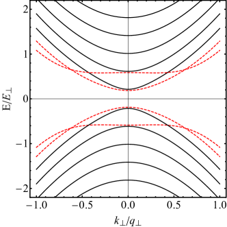
Figure 1: Subband dispersions of the harmonically confined 3D topological insulator. Left panel: Subbands obtained when both electron-hole asymmetry ($H_{\epsilon}$) and the $H_{\parallel}$-induced band mixing between the bare harmonic-oscillator subbands are neglected. Dashed curves indicate inverted bands. Right panel: Subbands calculated with only electron-hole asymmetry ($H_{\epsilon}$) neglected. In contrast to the case in the left panel, the lowest subband exhibits the expected dispersion of weakly hybridized massless-Dirac-like surface states. Parameters used in the calculations are $\gamma_{M_{0}}=-0.785$, $\gamma_{\parallel}=2.34$ (both correspond to Bi₂Se₃ [29]), and $\gamma_{\Omega}=0.400$.

While the oscillator subbands obtained from diagonalizing $H_{0}(-i\partial_{z},{\bm{\mathrm{k}}}_{\perp})+H_{V}(z)$ illustrate how confinement affects topological band inversion on a basic level, they can only yield a correct description when $H_{\parallel}(-i\partial_{z})$ is a small perturbation, i.e., in the confinement-dominated limit where $\gamma_{\parallel}\ll\gamma_{\Omega}$. In Bi₂Se₃, this is not the typical situation as $\gamma_{\parallel}=2.34$ is larger than any reasonably possible value for $\gamma_{\Omega}$, and the inclusion of $H_{\parallel}(-i\partial_{z})$ significantly affects the subband dispersions. Formally, the coupling of individual oscillator subbands by $H_{\parallel}(-i\partial_{z})$ as the 3D limit is approached has many similarities with the way models for 3D TIs have been constructed based on transversely coupled 2D TIs [31]. Using the eigenstates of $H_{0}(-i\partial_{z},{\bm{\mathrm{k}}}_{\perp})+H_{V}(z)$ as a basis, we are able to efficiently diagonalize the full Hamiltonian $H_{0}(-i\partial_{z},{\bm{\mathrm{k}}}_{\perp})+H_{\parallel}(-i\partial_{z})+H_{V}(z)$. See the Appendix for mathematical details and the right panel of Fig. 1 for illustrative results. Most crucially, the band mixing induced by $H_{\parallel}(-i\partial_{z})$ conspires to create the surface-state dispersion expected for a confined 3D TI in the large-width limit [18, 17, 19, 20, 21]. In contrast to Bi₂Se₃, the parameter $\gamma_{\parallel}$ is quite small for Bi₂Te₃ ($0.484$) and Sb₂Te₃ ($0.117$), as compared with the nominal maximum values of $\gamma_{\Omega}$ ($4$ and $3$) derived from equating $\sqrt{2}\,l_{\Omega}$ with their quintuple-layer width ($\approx 1$ nm). Hence, these materials should lend themselves to a more detailed exploration of the transition between the 3D-bulk and confinement-dominated regimes. The interactive simulations provided in the supplementary data for this article show the evolution of subband structure in confined TIs made from Bi₂Se₃, Bi₂Te₃, and Sb₂Te₃.

The fundamental gap $\Delta$ between the lowest conduction (sub-)band and the highest valence (sub-)band is a quantity of both conceptual and practical importance. It was shown to decrease exponentially as a function of system size in the confined direction both in 2D [22] and 3D [18, 17, 19, 20] TIs. For 3D TIs [18, 32, 33] and inversion-symmetry-breaking 2D TIs [34], the exponential decay of $\Delta$ was observed to be modulated by an oscillation. Within our model, we observe the oscillatory behavior, but with interesting materials-dependent features. See Fig. 2. The more strongly confinement-dominated materials Bi₂Te₃ and Sb₂Te₃ (those with a rather small magnitude of the parameter $\gamma_{\parallel}$) show clear oscillations, and the condition for the bare subband crossings, i.e., vanishing effective Dirac gap given in (1bcgf), quite accurately predicts the values of $\gamma_{\Omega}$ at which $\Delta$ is minimal. Thus the period of gap oscillations in these two materials is consistent with $\delta(1/\gamma_{\Omega})\sim 1/\gamma_{M_{0}}$, which corresponds to a period $\delta l_{\Omega}\sim\sqrt{M_{1}/M_{0}}$ for oscillation of the gap as a function of the effective 2D-system width scale $l_{\Omega}$. This estimate agrees with similar ones derived previously using a hard-wall confinement [25] and a tight-binding model [32], respectively, but deviations from such effective-Hamiltonian-based results occur in few-layer samples [35, 36, 29]. In contrast, no gap oscillations are discernible in our model with parameters applicable to Bi₂Se₃, for which the mixing of bare harmonic-oscillator subbands is always important due to the large value of $\gamma_{\parallel}$. Hence, even though transitions between normal and inverted phases occur typically for the 2D subbands in all three materials (see below), their heralding by gap oscillations depends sensitively on band-structure details [37] and, in contrast to expectation [32], is therefore not universal. The observed absence (presence) of gap oscillations in Bi₂Se₃ (Bi₂Te₃ and Sb₂Te₃) also suggests that the system is dominantly a strong (weak) TI [38].

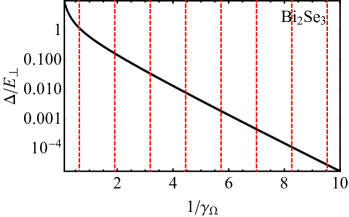
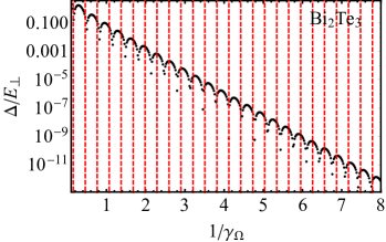
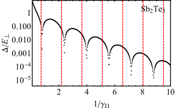
Figure 2: Confinement dependence of the band gap $\Delta$, calculated with $H_{\epsilon}$ neglected. The left (right, bottom) panel shows results obtained using the materials parameters [29] for Bi₂Se₃ (Bi₂Te₃, Sb₂Te₃), i.e., $\gamma_{M_{0}}=-0.785$ ($-3.27$, $-0.683$), $\gamma_{\parallel}=2.34$ ($0.484$, $0.117$). Vertical lines correspond to values of $\gamma_{\Omega}$ for which the confinement-renormalized effective gap $\Delta_{n{\bm{\mathrm{0}}}}$ given in Eq. (1bcgf) vanishes.

4 Confinement tuning of band inversion and surface-state hybridization

The band inversion in TI materials can be measured directly by the pseudo-spin projection of energy eigenstates. Within our present notation, ordinary conduction (valence) band character of a state is quantified by the expectation value $\langle{\tau_{z}\otimes\sigma_{0}}\rangle$ being close to $+1$ ($-1$). We use this measure to study the fate of band inversion in quantum-confined TI systems, complementing recent experimental studies [23]. Within our formalism where a general state is given as a superposition

$$\Psi_{{\bm{\mathrm{k}}}_{\perp}}(z)=\sum_{n\alpha}\left[b_{n{\bm{\mathrm{k}}}_{\perp}}^{(\alpha+)}\,\psi_{n{\bm{\mathrm{k}}}_{\perp}\alpha}(z)\otimes|{+}\rangle_{\mathrm{s}}+b_{n{\bm{\mathrm{k}}}_{\perp}}^{(\alpha-)}\,\psi^{\ast}_{n{\bm{\mathrm{k}}}_{\perp}\alpha}(z)\otimes|{-}\rangle_{\mathrm{s}}\right]\,,$$ (1bcgij)

its pseudo-spin expectation value is straightforwardly calculated as

$$\langle{\tau_{z}\otimes\sigma_{0}}\rangle_{{\bm{\mathrm{k}}}_{\perp}}=\sum_{n\alpha\beta}\Bigg{[}\sum_{\tau}\frac{\tau}{2}\left(1+\tau\,\frac{\Delta_{n{\bm{\mathrm{k}}}_{\perp}}}{E_{n{\bm{\mathrm{k}}}_{\perp}\alpha}}\right)^{\frac{1}{2}}\left(1+\tau\,\frac{\Delta_{n{\bm{\mathrm{k}}}_{\perp}}}{E_{n{\bm{\mathrm{k}}}_{\perp}\beta}}\right)^{\frac{1}{2}}\Bigg{]}\left[\sum_{\sigma}\Re\mathrm{e}\left\{\big{[}b_{n{\bm{\mathrm{k}}}_{\perp}}^{(\alpha\sigma)}\big{]}^{*}b_{n{\bm{\mathrm{k}}}_{\perp}}^{(\beta\sigma)}\right\}\right].$$

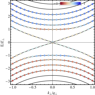
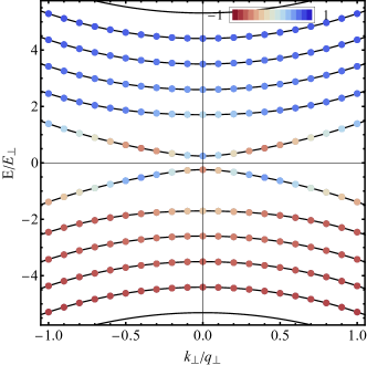
Figure 3: Band inversion in a harmonically confined 3D topological insulator with large band mixing ($\gamma_{\parallel}=2.34$ as for Bi₂Se₃ [29]) and electron-hole asymmetry neglected. The left (right) panel corresponds to $\gamma_{\Omega}=0.400$ ($0.900$). The color of a dot is a measure for the pseudo-spin expectation value $\langle{\tau_{z}\otimes\sigma_{0}}\rangle$ of the corresponding eigenstate as per the given scale. Subbands at large positive (negative) energies are found to have the ordinary conduction-(valence-)band character, as signified by a pseudo-spin value close to $+1$ ($-1$). Lower subbands in not-too-thin samples exhibit band inversion, as exemplified by the 2nd subband in the left panel. The interplay of band inversion and size quantization can also result in nontrivial $k_{\perp}$ dependences of the pseudo-spin projection, an example of which is shown by the lowest subband in the right panel. See also the simulations illustrating the evolution of subband structure and pseudo-spin character as the confinement-related parameter $\gamma_{\Omega}$ is varied continuously, which are provided as supplemental data.

As the thickness of the TI layer decreases, more and more 2D subbands (those with band index $n\gg n_{\mathrm{c}}$) show normal behavior, with conduction and valence band states having the ordinary pseudo-spin character. Low-energy subbands with $n\lesssim n_{\mathrm{c}}$ continue to have band inversion, but the lowest-energy ones become increasingly dominated by confinement effects and less by the band mixing arising from $H_{\parallel}$. In particular, the lowest subband oscillates between normal and inverted character in the strongly confinement-dominated regimes exhibited by Bi₂Te₃ and Sb₂Te₃. Figure 3 shows examples of such features using materials parameters applicable to Bi₂Se₃. More extensive simulations provided as supplementary data illustrate the evolution of band inversion as the confinement-related parameter $\gamma_{\Omega}$ is varied continuously in the three materials of interest. Generally, an oscillating change between normal and inverted character of the lowest subband is observed to follow the cycle of closings for the bare gap parameter $\Delta_{n{\bm{\mathrm{k}}}_{\perp}}$ from Eq. (1bcgf). To a lesser extent, this is the case for the not-confinement-dominated Bi₂Se₃. Generally, the magnitude of the gap appears to be more strongly affected by band mixing than the pseudo-spin character of the size-quantized subband states. Thus it can be misleading to use the measured sequence of gap minima to infer topological and normal regimes in a confined system, whereas the pseudo-spin always serves as a reliable identifier. The cycle of band inversions occurring in the bare harmonic-oscillator part of the model embodied in $H_{0}(-i\partial_{z},{\bm{\mathrm{k}}}_{\perp})+H_{V}(z)$ generally coincides quite well with the succession of band inversions for the lowest 2D subbands obtained from diagonalizing the full model $H_{0}(-i\partial_{z},{\bm{\mathrm{k}}}_{\perp})+H_{\parallel}(-i\partial_{z})+H_{V}(z)$.

Whether a 2D subband is inverted or normal is conventionally determined by the character of states at the band edges. At finite in-plane wave vector ${\bm{\mathrm{k}}}_{\perp}$, inter-band coupling due to the term proportional to $A_{0}$ in (1bb) induces a mixing of pseudo-spin states, and the term proportional to $M_{2}$ contributes to the effective band gap. As a result, a crossover from inverted to normal character generally occurs at large $k_{\perp}$, as can be seen for the first and second subbands shown in the left panel of Fig. 3. Interestingly, for low-lying 2D subbands and in the confinement-dominated regime, band inversion can also just occur within a region of finite $k_{\perp}$. See the right panel of Fig. 3 for a pertinent example, and the simulations provided as supplemental data for further illustration. Again, it should be emphasized that our results regarding the evolution of band inversions with quantum confinement are based on the effective-Hamiltonian approach from which we expect deviations to occur in few-layer samples [35, 36, 29].

In a thick sample, the lowest-lying subband corresponds to states localized at the system’s boundaries. As confinement is increased, i.e., sample thickness reduced, hybridization of states from opposite surfaces becomes important, and the states progressively loose their boundary-localized character. Eventually, even the lowest-lying subband-edge states are extended over the entire 2D-layer width. This general behavior is instructively demonstrated by the shape of probability-density distributions of lowest-subband-edge states shown as part of the interactive simulations provided in the supplementary data. To enable a more quantitative exploration of the transition between the boundary-localized and 2D-layer-extended regimes, we introduce $l_{\Omega}\,|\Psi_{{\bm{\mathrm{k}}}_{\perp}}(z)|^{2}$ for ${\bm{\mathrm{k}}}_{\perp}=0$ and $z=0$ as a measure for the hybridization-induced 2D-bulk character of subband-edge states. See Fig. 4. In Bi₂Se₃, small abrupt changes associated with band inversions occur on top of a systematic change to the strongly hybridized regime for $1/\gamma_{\Omega}\lesssim 3$. The practically vanishing hybridization for a broad range of confinement strengths is indicative of well-defined surface states. In contrast, the transition between surface-localized lowest-energy states to 2D-bulk-like behavior is sharper in the confinement-dominated case of Sb₂Te₃ but, at the same time, hybridization remains substantial even for the larger-thickness samples.

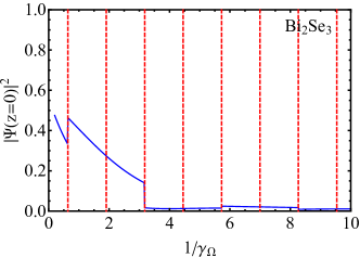
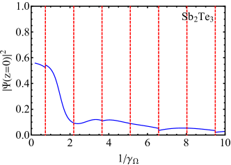
Figure 4: Transition from boundary-localized to 2D-layer-extended character of the lowest conduction subband-edge state, as measured by its probability density $|\Psi_{{\bm{\mathrm{k}}}_{\perp}=0}(z)|^{2}$ at the 2D layer’s center position $z=0$. The left (right) panel shows results calculated for Bi₂Se₃ (Sb₂Te₃) materials parameters [29] with electron-hole asymmetry neglected. Vertical lines correspond to values of $\gamma_{\Omega}$ for which the confinement-renormalized effective gap $\Delta_{n{\bm{\mathrm{0}}}}$ given in Eq. (1bcgf) vanishes.

5 Effect of electron-hole asymmetry

So far, we have neglected the influence of asymmetries between conduction and valence bands that are embodied in the contribution $H_{\epsilon}(k_{z},{\bm{\mathrm{k}}}_{\perp})$ to the TI-material Hamiltonian given in (1i). Comparing the magnitudes of $C_{1}$ and $C_{2}$ with those of $M_{1}$ and $M_{2}$, respectively, in real materials would suggest that electron-hole asymmetry is generally not a small effect. Here we investigate the latter’s influence on the modification of topological properties by quantum confinement.

The effect of the electron-hole-symmetry-breaking contribution $H_{\epsilon}(k_{z},{\bm{\mathrm{k}}}_{\perp})$ on the subband dispersions generally turns out to be indeed quite large, as a comparison of results corresponding to Bi₂Se₃ shown in the left panels of Figs. 3 and 5 clearly demonstrates. Most importantly, the position of the neutrality point for the massless-Dirac-like surface states is shifted in energy, and the conduction and valence subbands acquire different effective masses, even leading to a mass inversion occurring in a valence subband. Significant qualitative differences in the subband structure for Sb₂Te₃, shown in the right panel of Fig. 5, are a consequence of the different magnitudes and opposite sign for the bulk-bandstructure parameters entering $H_{\epsilon}(k_{z},{\bm{\mathrm{k}}}_{\perp})$.

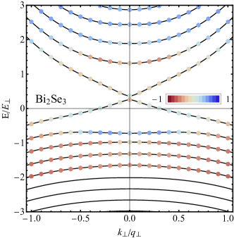
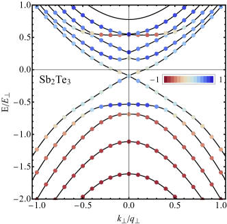
Figure 5: Effect of electron-hole asymmetry on subband dispersions and the pseudo-spin expectation value. The left (right) panel shows results calculated with band-structure parameters [29] for Bi₂Se₃ (Sb₂Te₃) and $\gamma_{\Omega}=0.400$.

Given the drastic changes exhibited in the lineshapes of subband spectra, one may ask whether, and if so how, any of the above-discussed features associated with the interplay of topological properties and quantum confinement survive in the presence of electron-hole asymmetry. We focus here specifically on the fundamental (i.e., lowest-subband energy) gap and the band inversion. Interactive simulations are included as supplemental data to visualize the situation. As it turns out, in the confinement-dominated regime, electron-hole asymmetry is found to lead only to marginal quantitative changes. Basic qualitative features such as gap oscillations and subband inversions occur very similarly to the situation where $H_{\epsilon}(k_{z},{\bm{\mathrm{k}}}_{\perp})$ is neglected, with the gap oscillations typically more significantly affected [37]. This is particularly clearly exhibited by the case of Sb₂Te₃ for not-too-weak confinement. But also for Bi₂Se₃ where mixing of bare-oscillator subbands is strong, the evolution of band inversions is basically identical with and without electron-hole asymmetry included, even for the lowest subband and weakest confinement strengths. Interestingly, for the system whose parameters correspond to Sb₂Te₃, the scrambling of low-energy subbands in the limit of very weak confinement tends to obscure the topological-insulator properties that are still unambiguously exhibited when electron-hole asymmetry is neglected.

6 Conclusions and outlook

We have used the effective-model description of bulk-TI band structures to investigate the effect of a soft, harmonic-oscillator-type, quantum confinement on physical properties that epitomize topological phases. Our study focuses explicitly on three materials systems (Bi₂Se₃, Bi₂Te₃ and Sb₂Te₃) that are representatives for quite different regions of the 3D-TI parameter space and, hence, exhibit distinctive features in the evolution of topological properties as the strength of the confinement is varied. Interactive simulations have been included as supplemental data to enable more detailed exploration of these differences. The results obtained here are also straightforwardly generalized to any materials systems whose band structure is described by the same type of ${\bm{\mathrm{k}}}\cdot{\bm{\mathrm{p}}}$ Hamiltonian that forms the basis for our theoretical approach, including Dirac semimetals [39, 40, 41] and other surmised TIs such as Bi₂Te₂I₂ [42].

The interplay of band inversion, size quantization, and band mixing is found to be governed by the relative magnitudes of unit-less parameters defined in Eq. (1bce). Characteristic features exhibited by the particular materials systems considered here can thus be rationalized in terms of the specific values of these parameters. Fundamentally, as the system size in the confined direction varies, the gaps of inverted bare-oscillator subbands [Eq. (1bcgf)] are successively closing and reopening. Mixing of bare-oscillator subbands significantly modifies the bare-oscillator subband dispersions in the large-width regime ($\gamma_{\Omega}<\gamma_{\parallel}$), establishing the vanishing-mass Dirac-like surface-state dispersion and eventually causing the disappearance of oscillations in the fundamental (lowest-subband) gap value. We track the evolution of band inversions by explicit consideration of the pseudo-spin value of eigenstates, establishing the robustness of TI phases with respect to band mixing and electron-hole asymmetry. In contrast, the occurrence of gap oscillations turns out to be a nonuniversal feature that is generally not a useful measure to monitor TI character in a quantum-confined system.

Our study considering 3D TIs subject to the harmonic-oscillator confining potential complements previous works that assumed hard-wall confinement. In contrast to the situation reported in single-particle analyses of 2D TIs [12, 13, 26], the basic features and overall trends associated with the effects of size quantization on 3D-TI properties do not drastically differ between the cases of hard-wall and soft-harmonic-oscillator potentials. Instead of the type of confining potential, differences in the 3D-TI bandstructure parameters are a major cause of significant variability in the exhibited behaviors.

The conclusions presented in this work have been reached based on an approach where certain aspects of real materials were ignored. One of these is the finite size of thin-film samples in the plane perpendicular to the quantum-confined direction and any effects arising from the conducting lateral surfaces. However, apart from the edge-state structure in strong perpendicular magnetic fields [43], systems with a large-enough aspect ratio are well-described by models assuming them to be infinite in the transverse directions. Another potentially relevant issue concerns the interplay of confinement and interactions. For example, the presence of long-range (Coulomb) interactions is known to induce a reconstruction of the boundary-electronic (edge-state) structure in 2D quantum-Hall [44, 45, 46, 47] and quantum-spin-Hall [27, 48] systems. Although interaction effects often turn out to be less pronounced in higher spatial dimensions, it would be interesting for future studies to address the influence of Coulomb interactions on harmonically confined 3D TIs, especially those where strong correlations are expected to affect topological properties [49, 50]. The goal of such investigations would be to establish how, and where in parameter space, the purely single-particle-related confinement effects in 3D TIs discussed in the present work are modified due to interactions.

Appendix

Here we provide some mathematical details for solving the Schrödinger problem for a quantum-confined 3D TI.

When electron-hole asymmetry is neglected, the Schrödinger equation reads

$$\left[H_{0}(-i\partial_{z},{\bm{\mathrm{k}}}_{\perp})+H_{\parallel}(-i\partial_{z})+H_{V}(z)\right]\Psi_{{\bm{\mathrm{k}}}_{\perp}}(z)=E_{{\bm{\mathrm{k}}}_{\perp}}\,\Psi_{{\bm{\mathrm{k}}}_{\perp}}(z)\quad.$$ (1bcgil)

Making the Ansatz (1bcgij) transforms (1bcgil) into a set of recursive relations

$$\frac{E_{m{\bm{\mathrm{k}}}_{\perp}\beta}-E_{{\bm{\mathrm{k}}}_{\perp}}}{E_{\perp}}\,b^{(\beta\sigma)}_{m{\bm{\mathrm{k}}}_{\perp}}+\sigma\,i\sum_{\alpha}\left[C^{m-1,m}_{\alpha\beta,{\bm{\mathrm{k}}}_{\perp}}\,\,b^{(\alpha,-\sigma)}_{m-1,{\bm{\mathrm{k}}}_{\perp}}+C^{m,m+1}_{\beta\alpha,{\bm{\mathrm{k}}}_{\perp}}\,\,b^{(\alpha,-\sigma)}_{m+1,{\bm{\mathrm{k}}}_{\perp}}\right]=0$$ (1bcgim)

for the unknown coefficients $b^{(\alpha\sigma)}_{n{\bm{\mathrm{k}}}_{\perp}}$, with the matrix elements given explicitly by

$$C^{n,m}_{\alpha\beta,{\bm{\mathrm{k}}}_{\perp}}=\sqrt{\frac{m\,\gamma_{\Omega}\,\gamma_{\parallel}}{8\,E_{n{\bm{\mathrm{k}}}_{\perp}\alpha}\,E_{m{\bm{\mathrm{k}}}_{\perp}\beta}}}\,\Bigg{[}\alpha\,\sqrt{\left(E_{m{\bm{\mathrm{k}}}_{\perp}\beta}+\Delta_{m{\bm{\mathrm{k}}}_{\perp}}\right)\left(E_{n{\bm{\mathrm{k}}}_{\perp}\alpha}-\Delta_{n{\bm{\mathrm{k}}}_{\perp}}\right)}$$

$$\hskip 113.81102pt-\beta\,\sqrt{\left(E_{m{\bm{\mathrm{k}}}_{\perp}\beta}-\Delta_{m{\bm{\mathrm{k}}}_{\perp}}\right)\left(E_{n{\bm{\mathrm{k}}}_{\perp}\alpha}+\Delta_{n{\bm{\mathrm{k}}}_{\perp}}\right)}\Bigg{]}\,\,.$$ (1bcgin)

We truncate this infinite set of equations by writing a matrix equation, $\mathcal{H}_{N}\,b_{N}=E_{N}\,b_{N}$, with $N$ large enough as required to achieve numerical accuracy, and the definitions

$$b_{N}=\left(b_{0,{\bm{\mathrm{k}}}_{\perp}}^{(++)},b_{0,{\bm{\mathrm{k}}}_{\perp}}^{(-+)},b_{0,{\bm{\mathrm{k}}}_{\perp}}^{(+-)},b_{0,{\bm{\mathrm{k}}}_{\perp}}^{(--)},b_{1,{\bm{\mathrm{k}}}_{\perp}}^{(++)},\dots,b_{N-1,{\bm{\mathrm{k}}}_{\perp}}^{(--)}\right)^{T}\quad,$$ (1bcgio)

$$\mathcal{H}_{N}=\left(\begin{array}[]{cccccccc}\mathcal{E}_{0}^{\prime}&\Gamma_{0}&&&&&&\\ (\Gamma_{0})^{\dagger}&\mathcal{E}_{1}^{\prime}&\Gamma_{1}&&&&0&\\ &(\Gamma_{1})^{\dagger}&\mathcal{E}_{2}^{\prime}&\Gamma_{2}&&&&\\ &&.&.&.&&&\\ &&&.&.&.&&\\ &0&&&.&.&.&\\ &&&&&(\Gamma_{N-2})^{\dagger}&\mathcal{E}_{N-1}^{\prime}&\Gamma_{N-1}\end{array}\right)\,,$$ (1bcgiw)

$$\mathcal{E}_{n}^{\prime}=\left(\begin{array}[]{cccc}E_{n{\bm{\mathrm{k}}}_{\perp}+}&0&0&0\\ 0&E_{n{\bm{\mathrm{k}}}_{\perp}-}&0&0\\ 0&0&E_{n{\bm{\mathrm{k}}}_{\perp}+}&0\\ 0&0&0&E_{n{\bm{\mathrm{k}}}_{\perp}-}\end{array}\right),\,\Gamma_{n}=\left(\begin{array}[]{cc}0&\mathrm{i}C_{n}\\ -\mathrm{i}C_{n}&0\end{array}\right),$$ (1bcgiad)

$$C_{n}=\left(\begin{array}[]{cc}C^{n,n+1}_{++,{\bm{\mathrm{k}}}_{\perp}}&C^{n,n+1}_{+-,{\bm{\mathrm{k}}}_{\perp}}\\[8.5359pt] C^{n,n+1}_{-+,{\bm{\mathrm{k}}}_{\perp}}&C^{n,n+1}_{--,{\bm{\mathrm{k}}}_{\perp}}\end{array}\right)\quad.$$ (1bcgiag)

For the case with electron-hole asymmetry included, the contribution $H_{\epsilon}\left(-i\partial_{z},{\bm{\mathrm{k}}}_{\perp}\right)$ from (1i) needs to be added to the Hamiltonian. As a result, the recursion relations (1bcgim) are modified and now read

$$\left[\frac{E_{m{\bm{\mathrm{k}}}_{\perp}\beta}-E_{{\bm{\mathrm{k}}}_{\perp}}}{E_{\perp}}+\gamma_{\epsilon}\,\gamma_{\Omega}\left(m+\frac{1}{2}\right)+\frac{C_{0}}{E_{\perp}}+\frac{C_{2}}{M_{2}}\,\frac{{\bm{\mathrm{k}}}_{\perp}^{2}}{q_{\perp}^{2}}\right]\,b^{(\beta\sigma)}_{m{\bm{\mathrm{k}}}_{\perp}}+\sum_{\alpha}\Big{[}\sigma\,i\,C^{m-1,m}_{\alpha\beta,{\bm{\mathrm{k}}}_{\perp}}\,\,b^{(\alpha,-\sigma)}_{m-1,{\bm{\mathrm{k}}}_{\perp}}$$

$$+\,\,\sigma\,i\,C^{m,m+1}_{\beta\alpha,{\bm{\mathrm{k}}}_{\perp}}\,\,b^{(\alpha,-\sigma)}_{m+1,{\bm{\mathrm{k}}}_{\perp}}+D^{m-2,m}_{\alpha\beta,{\bm{\mathrm{k}}}_{\perp}}\,\,b^{(\alpha,\sigma)}_{m-2,{\bm{\mathrm{k}}}_{\perp}}+D^{m,m+2}_{\beta\alpha,{\bm{\mathrm{k}}}_{\perp}}\,\,b^{(\alpha,\sigma)}_{m+2,{\bm{\mathrm{k}}}_{\perp}}\Big{]}=0\,\,\,,$$ (1bcgiah)

with $\gamma_{\epsilon}=C_{1}/(2M_{1})$ and

$$D^{n,m}_{\alpha\beta,{\bm{\mathrm{k}}}_{\perp}}=\frac{\gamma_{\epsilon}\,\gamma_{\Omega}\,\sqrt{m(n+1)}}{4\sqrt{E_{n{\bm{\mathrm{k}}}_{\perp}\alpha}E_{m{\bm{\mathrm{k}}}_{\perp}\beta}}}\Bigg{[}\sqrt{\left(E_{m{\bm{\mathrm{k}}}_{\perp}\beta}+\Delta_{m{\bm{\mathrm{k}}}_{\perp}}\right)\left(E_{n{\bm{\mathrm{k}}}_{\perp}\alpha}+\Delta_{n{\bm{\mathrm{k}}}_{\perp}}\right)}$$

$$\hskip 99.58464pt+\,\,\alpha\beta\,\sqrt{\left(E_{m{\bm{\mathrm{k}}}_{\perp}\beta}-\Delta_{m{\bm{\mathrm{k}}}_{\perp}}\right)\left(E_{n{\bm{\mathrm{k}}}_{\perp}\alpha}-\Delta_{n{\bm{\mathrm{k}}}_{\perp}}\right)}\Bigg{]}\quad.$$ (1bcgiai)

Consequently, this leads to an expression similar to (1bcgiw),

$$\mathcal{H}_{N}^{\epsilon}=\left(\begin{array}[]{ccccccccc}\mathcal{E}_{0}&\Gamma_{0}&\Delta_{0}&&&&&&\\ (\Gamma_{0})^{\dagger}&\mathcal{E}_{1}&\Gamma_{1}&\Delta_{1}&&&&0&\\ (\Delta_{0})^{\dagger}&(\Gamma_{1})^{\dagger}&\mathcal{E}_{2}&\Gamma_{2}&\Delta_{2}&&&&\\ &.&.&.&.&.&&&\\ &&.&.&.&.&.&&\\ &0&&.&.&.&.&.&\\ &&&&(\Delta_{N-3})^{\dagger}&(\Gamma_{N-2})^{\dagger}&\mathcal{E}_{N-1}&\Gamma_{N-1}&\Delta_{N-1}\end{array}\right)\,\,,$$ (1bcgiaq)

with

$$\mathcal{E}_{n}=\mathcal{E}_{n}^{\prime}+E_{\perp}\,\mathrm{diag}\left[\gamma_{\epsilon}\,\gamma_{\Omega}\,\left(n+\frac{1}{2}\right)+\frac{C_{0}}{E_{\perp}}+\frac{C_{2}}{M_{2}}\,\frac{{\bm{\mathrm{k}}}_{\perp}^{2}}{q_{\perp}^{2}}\right]\quad,$$ (1bcgiar)

$$\Delta_{n}=\left(\begin{array}[]{cc}D_{n}&0\\ 0&D_{n}\end{array}\right)\quad,\quad D_{n}=\left(\begin{array}[]{cc}D_{++,{\bm{\mathrm{k}}}_{\perp}}^{n,n+2}&D_{+-,{\bm{\mathrm{k}}}_{\perp}}^{n,n+2}\\[8.5359pt] D_{-+,{\bm{\mathrm{k}}}_{\perp}}^{n,n+2}&D_{--,{\bm{\mathrm{k}}}_{\perp}}^{n,n+2}\end{array}\right)\quad.$$ (1bcgiaw)

References

References

- [1] Hasan M Z and Kane C L 2010 Rev. Mod. Phys. 82 3045–3067
- [2] Qi X L and Zhang S C 2011 Rev. Mod. Phys. 83 1057–1110
- [3] Hasan M Z, Xu S Y and Bian G 2015 Phys. Scr. T164 014001
- [4] Chiu C K, Teo J C Y, Schnyder A P and Ryu S 2016 Rev. Mod. Phys. 88 035005
- [5] Ludwig A W W 2016 Phys. Scr. T168 014001
- [6] Kane C L and Mele E J 2005 Phys. Rev. Lett. 95 146802
- [7] Bernevig B A, Hughes T L and Zhang S 2006 Science 314 1757–1761
- [8] König M, Wiedmann S, Brüne C, Roth A, Buhmann H, Molenkamp L W, Qi X L and Zhang S C 2007 Science 318 766–770
- [9] Liu C, Hughes T L, Qi X, Wang K and Zhang S 2008 Phys. Rev. Lett. 100 236601
- [10] Knez I, Du R and Sullivan G 2011 Phys. Rev. Lett. 107 136603
- [11] Hasan M Z and Moore J E 2011 Annu. Rev. Cond. Mat. Phys. 2 55–78
- [12] Stanescu T D, Galitski V, Vaishnav J Y, Clark C W and Das Sarma S 2009 Phys. Rev. A 79 053639
- [13] Stanescu T D, Galitski V and Das Sarma S 2010 Phys. Rev. A 82 013608
- [14] Bermudez A, Mazza L, Rizzi M, Goldman N, Lewenstein M and Martin-Delgado M A 2010 Phys. Rev. Lett. 105 190404
- [15] Goldman N, Satija I, Nikolic P, Bermudez A, Martin-Delgado M A, Lewenstein M and Spielman I B 2010 Phys. Rev. Lett. 105 255302
- [16] Béri B and Cooper N R 2011 Phys. Rev. Lett. 107 145301
- [17] Liu C X, Zhang H, Yan B, Qi X L, Frauenheim T, Dai X, Fang Z and Zhang S C 2010 Phys. Rev. B 81 041307
- [18] Linder J, Yokoyama T and Sudbø A 2009 Phys. Rev. B 80 205401
- [19] Lu H Z, Shan W Y, Yao W, Niu Q and Shen S Q 2010 Phys. Rev. B 81 115407
- [20] Shan W Y, Lu H Z and Shen S Q 2010 New J. Phys. 12 043048
- [21] Zhang F, Kane C L and Mele E J 2012 Phys. Rev. B 86 081303
- [22] Zhou B, Lu H Z, Chu R L, Shen S Q and Niu Q 2008 Phys. Rev. Lett. 101 246807
- [23] Salehi M, Shapourian H, Koirala N, Brahlek M J, Moon J and Oh S 2016 Nano Lett. 16 5528–5532
- [24] Zhang H, Liu C X, Qi X L, Dai X, Fang Z and Zhang S C 2009 Nat. Phys. 82 438–442
- [25] Liu C X, Qi X L, Zhang H, Dai X, Fang Z and Zhang S C 2010 Phys. Rev. B 82 045122
- [26] Buchhold M, Cocks D and Hofstetter W 2012 Phys. Rev. A 85 063614
- [27] Wang J, Meir Y and Gefen Y 2017 Phys. Rev. Lett. 118 046801
- [28] Orlita M, Piot B A, Martinez G, Kumar N K S, Faugeras C, Potemski M, Michel C, Hankiewicz E M, Brauner T, Drašar Č, Schreyeck S, Grauer S, Brunner K, Gould C, Brüne C and Molenkamp L W 2015 Phys. Rev. Lett. 114 186401
- [29] Nechaev I A and Krasovskii E E 2016 Phys. Rev. B 94 201410
- [30] Zhang G, Qin H, Teng J, Guo J, Guo Q, Dai X, Fang Z and Wu K 2009 Appl. Phys. Lett. 95 053114
- [31] Kobayashi K, Yoshimura Y, Imura K I and Ohtsuki T 2015 Phys. Rev. B 92 235407
- [32] Ozawa H, Yamakage A, Sato M and Tanaka Y 2014 Phys. Rev. B 90 045309
- [33] Betancourt J, Li S, Dang X, Burton J D, Tsymbal E Y and Velev J P 2016 J. Phys.: Condens. Matter 28 395501
- [34] Takagaki Y 2014 Phys. Rev. B 90 165305
- [35] Förster T, Krüger P and Rohlfing M 2015 Phys. Rev. B 92 201404
- [36] Förster T, Krüger P and Rohlfing M 2016 Phys. Rev. B 93 205442
- [37] Okamoto M, Takane Y and Imura K I 2014 Phys. Rev. B 89 125425
- [38] Imura K I, Okamoto M, Yoshimura Y, Takane Y and Ohtsuki T 2012 Phys. Rev. B 86 245436
- [39] Wang Z, Weng H, Wu Q, Dai X and Fang Z 2013 Phys. Rev. B 88 125427
- [40] Xiao X, Yang S A, Liu Z, Li H and Zhou G 2015 Sci. Rep. 5 7898
- [41] Pan H, Wu M, Liu Y and Yang S A 2015 Sci. Rep. 5 14639
- [42] Nechaev I A, Eremeev S V, Krasovskii E E, Echenique P M and Chulkov E V 2017 Sci. Rep. 7 43666
- [43] Liu Z, Jiang L and Zheng Y 2016 J. Phys.: Condens. Matter 28 275501
- [44] Dempsey J, Gelfand B Y and Halperin B I 1993 Phys. Rev. Lett. 70 3639–3642
- [45] MacDonald A H, Yang S R E and Johnson M D 1993 Aust. J. Phys. 46 345–358
- [46] Chamon C d C and Wen X G 1994 Phys. Rev. B 49 8227–8241
- [47] Barlas Y, Joglekar Y N and Yang K 2011 Phys. Rev. B 83 205307
- [48] Amaricci A, Privitera L, Petocchi F, Capone M, Sangiovanni G and Trauzettel B 2017 Phys. Rev. B 95 205120
- [49] Hohenadler M and Assaad F F 2013 J. Phys.: Condens. Matter 25 143201
- [50] Amaricci A, Budich J C, Capone M, Trauzettel B and Sangiovanni G 2016 Phys. Rev. B 93 235112
- [51] Nöckel J U [accessed 21-11-2016] URL http://mathematica.stackexchange.com/questions/18257/how-to-translate-interactive-graphics-from-mathematica-to-standard-htmlsvg