Mean-Field Theory of Water-Water Correlations in Electrolyte Solutions

Abstract

Long-range ion induced water-water correlations were recently observed in femtosecond elastic second harmonic scattering experiments of electrolyte solutions. To further the qualitative understanding of these correlations, we derive an analytical expression that quantifies ion induced dipole-dipole correlations in a non-interacting gas of dipoles. This model is a logical extension of Debye-Hückel theory that can be used to qualitatively understand how the combined electric field of the ions induces correlations in the orientational distributions of the water molecules in an aqueous solution. The model agrees with results from molecular dynamics simulations and provides an important starting point for further theoretical work.

The electric field of a solvated ion in water induces orientational ordering in the surrounding solvent molecules. However, the length scale over which this ordering persists has been a topic of significant debate, at least in part because the range at which correlations can be detected depends on the experimental probe.Marcus (2009) The results of neutron diffraction,Howell and Neilson (1996); Soper and Weckström (2006) X-ray scattering,Bouazizi et al. (2006); Bouazizi and Nasr (2007) dielectric relaxation,Buchner, Hefter, and May (1999) and femtosecond pump-probe experiments,Omta et al. (2003) as well as atomistic simulations of the reorientation timescales of water moleculesStirnemann et al. (2013) and of the vibrational spectrum of solutions,Smith, Saykally, and Geissler (2007); Funkner et al. (2012) have suggested that the ordering of the surrounding water molecules by ions extends no further than about 3 solvation shells (around 0.8 nm) for sub-molar concentrations. On the other hand, infrared photodissociation experiments,O’Brien et al. (2010); O’Brien and Williams (2012) and a study combining terahertz and femtosecond infrared spectroscopies,Tielrooij et al. (2010) have found evidence for ordering extended to longer ranges. Molecular dynamics simulations looking directly at the orientational correlations between water molecules showed that the presence of ionic solutes have an effect on these correlations at distances of more than 1 nm.Zhang and Galli (2014)

Femtosecond elastic second harmonic scattering (fs-ESHS)Shen (1989); Roke and Gonella (2012) measurements have recently been used to probe the orientational order of water molecules in H₂O and D₂O electrolyte solutions,Chen et al. (2016) revealing intensity changes that are already detectable at micromolar concentrations, and which are identical for more than 20 different electrolytes. The non-specificity of the fs-ESHS response, its magnitude, and its onset at low concentration point to its long-range origin. The isotope exchange experiment, together with the recorded polarization combinations (in conjunction with the selection rules for nonlinear light scattering experiments Bersohn, Pao, and Frisch (1966); Roke and Gonella (2012)) show that the recorded changes in the fs-ESHS response in the concentration range from 1 $\mu$M - 100 mM arise from water-water correlations that are induced by the ions (and not from the ions themselves). This effect shows intriguing correlations with changes in the surface tension of dilute electrolyte solutions, suggesting that the same microscopic phenomenon underlying the second-harmonic signal can have an impact on macroscopic observables.

In this Communication we derive an analytical expression for the correlations induced in a non-interacting gas of dipoles by the electric field of ions. This expression is a natural extension to a simple Debye-Hückel model, which has been shown to qualitatively capture the concentration-dependence of the second-harmonic response,Shelton (2009); Chen et al. (2016) and can be used to elucidate the nature, the range and the energetics of the weak ion-induced ordering probed by fs-ESHS. The expression provides a benchmark for a fundamental understanding of the interplay of ion-dipole and ion-ion interactions. By comparison with classical molecular dynamics simulations of dilute NaCl solutions, we demonstrate that both of these factors are needed to characterize the ion-induced solvent correlations.

We begin by considering the water molecules in an ionic solution to be point dipoles that interact only with the solute, and have no explicit dipole-dipole interactions. Thus, the orientational ordering of these dipoles is caused only by the electric field due to the ions. Although this might appear to be a harsh assumption – and it certainly implies that the model cannot report on short-ranged hydrogen-bonding and dipole-dipole interactions – the dipolar screening is implicitly included through macroscopic quantities such as the dielectric constant and the local field factor. We will also show later that dipole-dipole interactions can be included in a refined version of the model, and have no impact on the long-range behavior.

Figs. 1(a) and (b) show how this model is built up: firstly, the ions are taken to be point charges in a dielectric continuum, with an appropriate spatial distribution, after which the system is filled with a uniform gas of independent dipoles,Shelton (2009) which will align with the local electric field. We then define the dipole correlation function for two solvent molecules separated by a distance $r$ (that is, the average inner product of two dipoles as a function of their separation),

$$\left\langle\cos\phi\right\rangle(r)=\frac{1}{V}\int_{V}\left\langle\boldsymbol{\hat{\mu}}(\boldsymbol{R})\cdot\boldsymbol{\hat{\mu}}(\boldsymbol{R}+\boldsymbol{r})\right\rangle_{\text{o+i}}\,{\rm d}^{3}\boldsymbol{R},$$ (1)

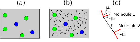
Figure 1: Illustration of the mean-field model considered in this communication: (a) ions are embedded in a dielectric continuum, and then (b) a uniform gas of independent point dipoles is added to the system. (c) Dipole correlation function $\left\langle\cos\phi\right\rangle(r)$: $r$ is the distance between two dipoles, $\boldsymbol{\mu}_{1}$ and $\boldsymbol{\mu}_{2}$ are their dipole moment vectors and $\cos\phi=\hat{\boldsymbol{\mu}}_{1}\cdot\hat{\boldsymbol{\mu}}_{2}$.

where $\boldsymbol{\hat{\mu}}(\boldsymbol{R})$ is the unit vector in the direction of the dipole moment of a molecule at $\boldsymbol{R}$, $V$ is the volume of the system and “o+i” denotes an average over molecular orientations and ionic positions. Fig. 1(c) illustrates how the angle $\phi$ is defined for two representative water molecules.

In the Supplementary Information (SI), we show that by taking a Taylor expansion in the reciprocal temperature $\beta=1/k_{\rm B}T$, we can make the approximation,

$$\left\langle\cos\phi\right\rangle(r)\simeq\frac{1}{V}\left(\frac{\beta\mu}{3}\right)^{2}\int_{V}\left\langle\boldsymbol{E}(\boldsymbol{R})\cdot\boldsymbol{E}(\boldsymbol{R}+\boldsymbol{r})\right\rangle_{\text{i}}\,{\rm d}^{3}\boldsymbol{R},$$ (2)

where $\boldsymbol{E}(\boldsymbol{R})$ is the total electric field at position $\boldsymbol{R}$ due to all of the ions in the solution, and $\mu$ is the permanent dipole moment of a water molecule. The subscript “i” indicates that the average is taken over the positions of ions. For simplicity of notation, any angular brackets in the following work without a subscript are taken over ion positions only. Eqn. (2) shows that in our model the correlation between dipoles is proportional to the correlation between electric fields, which are taken to be the only source of ordering for the molecules.

The electric field $\boldsymbol{E}(\boldsymbol{R})$ at a given position is the sum of electric fields due to all of the ions. This allows us to write,

$$\boldsymbol{E}(\boldsymbol{R})=\sum_{m\in\text{ions}}\frac{eZ_{m}f_{0}}{4\pi\epsilon_{0}\epsilon_{\rm r}}\boldsymbol{\mathcal{E}}(\boldsymbol{R}-\boldsymbol{r}_{m}),$$ (3)

with $Z_{m}$ the charge of the $m^{\rm th}$ ion in units of the electron charge $e$ and $\boldsymbol{r}_{m}$ the position of this ion, $f_{0}$ the Onsager local field factor,Onsager (1936) $\epsilon_{0}$ the vacuum permittivity, $\epsilon_{\rm r}$ the solvent dielectric constant, and $\boldsymbol{\mathcal{E}}(\boldsymbol{r})$ the electric field associated with individual ions (most commonly the Coulomb field, $\boldsymbol{r}/{r^{3}}$). This gives

$$\left\langle\cos\phi\right\rangle(r)\simeq\\ \frac{A}{V}\sum_{m,n}Z_{m}Z_{n}\int_{V}\left\langle\boldsymbol{\mathcal{E}}(\boldsymbol{R}-\boldsymbol{r}_{m})\cdot\boldsymbol{\mathcal{E}}(\boldsymbol{R}+\boldsymbol{r}-\boldsymbol{r}_{n})\right\rangle\,{\rm d}^{3}\boldsymbol{R},$$ (4)

in which we have defined $A=\left(\frac{\beta\mu f_{0}e}{12\pi\epsilon_{0}\epsilon_{\rm r}}\right)^{2}$.

In the thermodynamic ($V\rightarrow\infty$) limit the integral in Eqn. (4) is taken over all space and can be most conveniently expressed in reciprocal space,

$$\left\langle\cos\phi\right\rangle(r)\simeq\\ \frac{A}{V}\int\boldsymbol{\mathcal{E}}(\boldsymbol{K})\cdot\boldsymbol{\mathcal{E}}(-\boldsymbol{K})\left\langle\sum_{m,n}Z_{m}Z_{n}e^{i\boldsymbol{K}\cdot\left(\boldsymbol{r}_{m}-\boldsymbol{r}_{n}\right)}\right\rangle e^{i\boldsymbol{K}\cdot{\boldsymbol{r}}}\,\frac{{\rm d}^{3}\boldsymbol{K}}{\left(2\pi\right)^{3}},$$ (5)

where $\boldsymbol{\mathcal{E}}(\boldsymbol{K})$ is the Fourier transform of the field function $\boldsymbol{\mathcal{E}}(\boldsymbol{r})$. The term in angular brackets is proportional to the charge-charge structure factor $S(\boldsymbol{K})$ of the ions.Barrat and Hansen (2003) This gives the dipole correlation function in terms of the ion number density $\rho$ as,

$$\left\langle\cos\phi\right\rangle(r)\simeq\\ \frac{\rho}{\left(2\pi\right)^{3}}\left(\frac{\beta\mu ef_{0}}{12\pi\epsilon_{0}\epsilon_{\rm r}}\right)^{2}\int\left|\boldsymbol{\mathcal{E}}(\boldsymbol{K})\right|^{2}S(\boldsymbol{K})e^{i\boldsymbol{K}\cdot\boldsymbol{r}}\,{\rm d}^{3}\boldsymbol{K}.$$ (6)

The most appropriate mean-field model can be obtained by taking the field function $\boldsymbol{\mathcal{E}}(\boldsymbol{r})$ to be the Coulomb field $\boldsymbol{r}/r^{3}$ (corresponding to $\boldsymbol{\mathcal{E}}(\boldsymbol{K})=-4\pi i\boldsymbol{K}/K^{2}$), and using the Debye-Hückel (DH) structure factor Barrat and Hansen (2003) $S(K)=\frac{2K^{2}}{K^{2}+\kappa^{2}}$, where $\kappa=\left(\frac{2\rho\beta Z^{2}e^{2}}{\epsilon_{0}\epsilon_{\rm r}}\right)^{1/2}$ is the inverse Debye length. This gives

$$\left\langle\cos\phi\right\rangle_{\text{\tiny{DH}}}(r)=\frac{\rho}{2\pi}\left(\frac{\beta\mu ef_{0}}{3\epsilon_{0}\epsilon_{\rm r}}\right)^{2}\frac{e^{-\kappa r}}{r}.$$ (7)

The variation of $\left\langle\cos\phi\right\rangle_{\text{\tiny{DH}}}(r)$ with ion concentration is instructive. As seen in Figure 2, for small $\rho$, an increase in concentration leads to an increase in correlation between solvent dipoles, while for large $\rho$ the $e^{-\kappa r}$ factor dominates. Increasing the concentration results in ions being more screened and with a lesser propensity to orient solvent dipoles. It should be also noted that, at all of the concentrations shown in Fig. 2, the dipolar correlations at distances above 5 nm are very small. However, because the number of water molecules further than 5 nm away is very large, these correlations can be measured by fs-ESHS experiments, a testimony to the exquisite sensitivity of the probe.

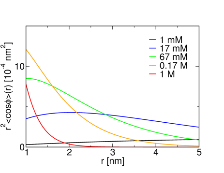
Figure 2: Solvent dipole-dipole correlation functions predicted by Eqn. (7) at different concentrations.

Eqn. (6) allows us to investigate the interplay between the ion-ion spatial correlations (encoded in $S(\boldsymbol{K})$) and the ion-dipole orientational correlations (due to the electric field $\boldsymbol{\mathcal{E}}(\boldsymbol{r})$). By changing the form of $S(\boldsymbol{K})$, one can estimate the response to an arbitrary distribution of ions: for instance, one could extend this model to investigate the correlations induced by charges on an interface. A particularly instructive example involves a completely uncorrelated arrangement of ions. This random-ion (RI) model is equivalent to setting $S(\boldsymbol{K})=2$, which leads to dipole-dipole correlations corresponding to Eqn. (7) with $\kappa=0$, while the concentration $\rho$ is kept constant. At all concentrations, this RI model leads to increased dipole-dipole correlations, because of the lack of screening of the Coulombic ion-dipole interaction by the correlated cloud of counterions. It is worth stressing that, although it might be appealing to qualitatively discuss the dampening of correlations in terms of the exponentially-screened DH field of an ion, this is not an appropriate model. Such a screened-field/random ions (SF-RI) model amounts to setting $\boldsymbol{\mathcal{E}}(\boldsymbol{r})=-\nabla\,\frac{e^{-\kappa r}}{r}=\boldsymbol{r}\left(\frac{e^{-\kappa r}}{r^{3}}+\frac{\kappa e^{-\kappa r}}{r^{2}}\right)$ and $S(\boldsymbol{K})=2$. The resulting functional form of the induced dipole-dipole correlations resembles that of the full DH model at short distances, but then leads to unphysical anticorrelations at large distance (see the SI).

Fig. 3 compares the predicted $\left\langle\cos\phi\right\rangle(r)$ using the full DH theory, the RI and the SF-RI models, and the correlations computed from a MD simulation using a $\sim$ 20 nm cubic box with about 264,000 TIP4P/2005 water molecules.Chen et al. (2016) All curves correspond to a salt concentration of 8 mM and a temperature of 300 K. The other physical constants used are described in the SI. Comparison with MD results in Fig. 3 shows that only the full DH model captures the correct long-range behavior of the dipole-dipole correlations – although the short range structure is clearly absent. Neglecting ion-ion spatial correlations artificially increases the orientational correlations, since randomly distributed ions cannot efficiently screen the fields of other ions. A picture in which one interprets dipole-dipole correlations in terms of the screened electrostatic field of the ions, while providing a qualitative picture of the physics, is inconsistent with the linearized-Boltzmann structure of the mean-field model, and fails to quantitatively reproduce the MD results. This comparison demonstrates that the long-ranged dipole-dipole correlations are most naturally interpreted as being due to the bare electric field of the ions. The correlations are modulated by short range interactions (which are not included in this model), and by the presence of ion-ion spatial correlations, which result in the screening of the Coulomb field. This latter effect leads to decreased dipole-dipole correlations and provides an explanation for the saturation of the fs-ESHS signal at high electrolyte concentrations.

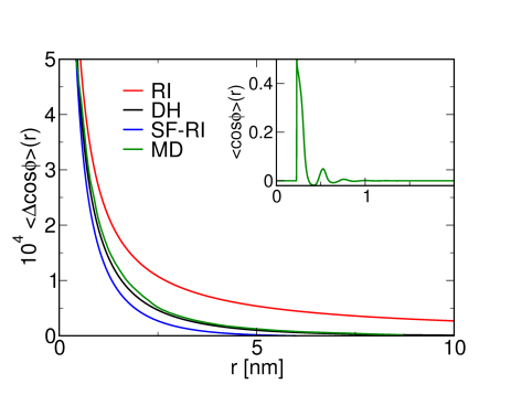
Figure 3: Comparison of the solvent dipole correlation function for the full Debye-Hückel theory (black line), the random-ion approximation (red line) and the screened-field plus random-ion approximation (blue line), with a salt concentration of 8 mM at $T=300$ K. We also show the correlation function calculated from MD at this concentration (green line). In all cases we have subtracted the correlation function for pure water at the same temperature. Note that this correlation is zero for the mean-field model, and so $\left\langle\Delta\cos\phi\right\rangle(r)=\left\langle\cos\phi\right\rangle(r)$ for all curves but MD. Inset: the absolute correlation function $\left\langle\cos\phi\right\rangle(r)$ calculated from MD, showing considerable structure at short range.

We note that the mean-field model can be further improved to include more physical effects. $\left\langle\cos\phi\right\rangle_{\text{\tiny{DH}}}(r)$ diverges in the $r\rightarrow 0$ limit because of the singularity in the electric field at the ion positions. It is possible to remove this short-distance divergence by restricting the volume of space in which water molecules can be found; however, the fact that two water molecules have a distance of minimum approach, below which $\left\langle\cos\phi\right\rangle(r)$ is not meaningful, makes the divergence irrelevant. We can also estimate the impact of neglecting dipole-dipole interactions, by re-introducing them in a perturbative fashion. This can be done by following the procedure used to derive the approximation in Eqn. (2), including also the dipole-dipole interaction. In doing so, we find (as described in the SI) that the lowest-order term in $\left\langle\cos\phi\right\rangle(r)$ that includes the dipole-dipole forces is proportional to $\beta^{4}e^{-\kappa r}/r^{7}$. This term decays much more rapidly than does the model of Eqn. (7), and makes essentially no contribution at long enough distances: above 0.33 nm, the magnitude of this correction is less than 1 % of the magnitude of $\left\langle\cos\phi\right\rangle_{\text{\tiny{DH}}}(r)$, and less than $10^{-3}$ % above 1 nm.

The computed residual orientational correlation of dipoles at a distance of several nm is extremely small, but since it involves many dipoles the total change in free energy may be non-negligible. In order to elucidate the free energy scale associated with ion-induced long-range dipole-dipole correlations, we evaluate the total energetic contribution associated with the oriented dipoles at distances larger than a chosen cut-off length $r_{\text{c}}$, which reads (see the SI), Hill (1986)

$$U=4\pi\rho_{\rm S}\mu\int_{r_{\rm c}}^{\infty}r^{2}E(r)\mathcal{L}\left(\beta\mu E(r)\right)\,{\rm d}r,$$ (8)

where $\mathcal{L}(x)=\coth(x)-1/x$ is the Langevin function and $\rho_{\rm S}$ is the solvent density. The mean electric field $E(r)$ around an ion is given by Debye-Hückel theory. The integral can be computed by expanding the integrand as a Taylor series in $\beta$.

Fig. 4 shows the total energetic contribution of the dipoles oriented by an ion as a function of the electrolyte concentration and for different cut-off distances. At mM concentrations, dipolar order beyond the Bjerrum length ($\sim 0.7$ nm in water at 300 K) is associated with an energy scale of about 3 $k_{B}T$, and even the tails beyond 4 nm correspond to a significant fraction of $k_{B}T$. Due to the large number of dipoles in the far region, the collective effect is significant even though each ion-dipole interaction is very small. Thus, it is plausible that ion-induced dipole-dipole correlations extending well beyond the Bjerrum length could lead to measurable changes in the macroscopic energy (as observed in the surface tension measurements of Ref. Chen et al., 2016). As this analysis is performed with a very simplified model, this conclusion is not definitive, and a more quantitative analysis should include changes in the long-range dipole-dipole order in the bulk and in the surface region. These changes could then be connected to changes in the free energy of the surface and the bulk region.

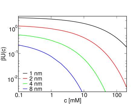
Figure 4: Energy of the dipoles oriented by a single ion as a function of ion concentration, for varying short-range cutoff distances $r_{\rm c}$.

In conclusion, we have shown that long-range, non-specific electrolyte-induced correlations in water as recently observed in fs-ESHS experiments can be captured by a simple mean-field model that treats water molecules as non-interacting dipoles oriented by the electrostatic field of ions, which are themselves correlated following Debye-Hückel theory. Although one can intuitively understand the orientational correlations as arising from the exponentially-screened field of correlated ions, a more accurate picture, leading to quantitative predictions of MD simulations, regards them as arising from unscreened ion-dipole correlations that combine destructively when the physically relevant ion-ion correlations are included. This model is very useful to pinpoint what we think is the main physical origin of the electrolyte-induced change in the fs-ESHS intensity and to estimate the length and energy scale of the effect. It does not, however, explain the dramatic isotope effects that are seen in experiments,Chen et al. (2016) or the temperature dependence of the fs-ESHS signal. As such it is clearly only a first step in a complete description of the experimental data, which should also include a re-evaluation of the molecular hyperpolarizability tensor,Tocci et al. (2016) particularly when probed by femtosecond laser pulses.Liang et al. (2017)

Supplementary Information

See supplementary information for more detailed derivations of the formulas used in the main text, as well as a list of the numerical values of physical constants used.

in 1,2,3,4,5,6,7,8,9 See pages \x of SI