Model atmospheres of sub-stellar mass objects

Abstract

We present an outline of basic assumptions and governing structural equations describing atmospheres of substellar mass objects, in particular the extrasolar giant planets and brown dwarfs. Although most of the presentation of the physical and numerical background is generic, details of the implementation pertain mostly to the code CoolTlusty. We also present a review of numerical approaches and computer codes devised to solve the structural equations, and make a critical evaluation of their efficiency and accuracy.

1 Introduction

There have been a number of theoretical studies dealing with constructing model atmospheres of the sub-stellar mass objects (SMO), most notably extrasolar giant planets (EGP) and brown dwarfs. In the context of EGPs, the first self-consistent model atmospheres were produced by Seager & Sasselov (1998), followed by Goukenleuque et al. (2000) and Barman et al. (2001). The first extended grid of EGP model atmospheres was constructed by Sudarsky et al. (2003). There have been many more theoretical studies afterward, but it is not our aim here to provide a historical review of the field.

Most of the literature deals with the properties of constructed models and with analyses of observations. However, the basic physical assumptions and the methodology of model construction is usually covered only in short sections, usually referring to other papers, or is sometimes lost in Appendices of otherwise application minded papers.

Here, we intend to fill this gap, and provide a systematic overview of basic physical assumptions, structural equations, and numerical methods to solve them. We also would like to clarify some previously confusing points, because researchers in the field of extrasolar giant planets come from both the planetary science and the stellar atmosphere communities and use their respective traditional terminologies, sometimes using the same term (e.g., the effective temperature, albedo, etc.) to mean a completely different concept.

Section 2 of this paper contains an outline of the basic assumptions and governing structural equations describing an SMO atmosphere. Section 3 then reviews the essential elements of the numerical methods used to solve the structural equations without unnecessary approximations, and Section 4 deals with some important details of the numerical procedure. Section 5 briefly discusses the topic of approximate, gray or pseudo-gray, models. They are useful as initial models for a subsequent iterative scheme to solve the structural equations exactly, as well as a pedagogical tool to understand the atmospheric temperature structure. Finally, in Section 6, we discuss a comparison of the present scheme to other modeling approaches. We also include several Appendices where some technical details are described.

We stress that while Section 2 presents a general outline of the physical background which is largely universal and is adopted by a number of approaches and computer codes, the material presented in Sections. 3 and 4 pertains mostly to the code CoolTlusty (Hubeny et al. 2003, Sudarsky et al . 2003) which was developed as a variant of the universal stellar atmosphere code tlusty (Hubeny 1988, Hubeny & Lanz 1995), although analogous or similar techniques are adopted in other codes, as is summarized in Section 6.

2 Physical background

We will describe here a procedure to compute the so-called classical model atmospheres; that is, plane-parallel, horizontally homogeneous atmospheres in hydrostatic and radiative (or radiative+convective) equilibrium.

The basic physical framework employed to model the atmospheres of SMOs represents a straightforward extension of the physical description used in the theory of stellar atmospheres. For a comprehensive discussion and detailed description of the basic physics and numerics in the stellar context, refer to Hubeny & Mihalas (2014; in particular Chaps. 12–13, 16–18).

2.1 Basic structural equations

The basic structural equations are the hydrostatic equilibrium equation and the energy balance equation, Since radiation critically influences the energy balance, the radiative transfer equation has to be viewed as one of the basic structural equations. These equations are supplemented by the equation of state and the equations that define the absorption and emission coefficient for radiation. We shall briefly discuss these equations below.

2.1.1 Radiative transfer equation

For a time-independent, horizontally homogeneous atmosphere, possibly irradiated by an external source which is symmetric with respect to the normal to the surface, the radiative transfer equation is written as

$$\mu\frac{dI(\nu,\mu,z)}{dz}=-\chi(\nu,z)I(\nu,\mu,z)+\eta^{\rm tot}(\nu,\mu,z),$$ (2.1)

where $I$ is the specific intensity of radiation defined such as $I\cos\theta\,d\nu dtdSd\Omega$ is the energy of radiation having a frequency in the range $(\nu,\nu+d\nu)$ going through an elementary surface $dS$ in an element of solid angle $d\Omega$ around direction of propagation ${\bf n}$, with angle $\theta$ between the normal to the surface element $dS$, and ${\bf n}$, in time interval $dt$. In the plane-parallel geometry, the state parameters depend only on one geometrical coordinate, the depth in the atmosphere, and the specific intensity depends only on the angle $\theta$; we use a customary notation $\mu\equiv\cos\theta$.

Further, $\chi$ and $\eta^{\rm tot}$ are the total absorption and emission coefficients, respectively. They include both the thermal as well as the scattering processes – see below. Here we assume that there are no external forces and no macroscopic velocities, so the absorption coefficient does not depend on $\mu$. The emission coefficient may still depend on direction; however, for an isotropic scattering the emission coefficient is also independent of $\mu$, $\eta^{\rm tot}(\nu,\mu,z)=\eta^{\rm tot}(\nu,z)$.

In the following, we denote a dependence on frequency through index $\nu$ and omit an indication of the dependence on depth. The total absorption coefficient, or extinction coefficient, is written as

$$\chi_{\nu}=\kappa_{\nu}+s_{\nu},$$ (2.2)

where $\kappa_{\nu}$ is the coefficient of true absorption, which correspond to a process during which an absorbed photon is destroyed, while $s_{\nu}$ is is the scattering coefficient, corresponding to a process which removes a photon from the beam, but re-emits it in a different direction We note that this coefficient is sometime denoted as $\sigma_{\nu}$, but we use the notation with $s$ to avoid a confusion with cross sections which we denote $\sigma$ – see below.

The total emission coefficient is also given as a sum of thermal and scattering contributions. The latter refers only to continuum scattering; scattering. In the context of SMO model atmospheres, spectral lines are treated with complete frequency redistribution, in which case the scattering term is in fact a part of the thermal emission coefficient. The continuum scattering part is usually treated separately from the thermal part, and the “thermal emission coefficient” is usually called the “emission coefficient.” Specifically, the total emission coefficient is written as

$$\eta_{\nu}^{\rm tot}=\eta_{\nu}+\eta_{\nu}^{\rm sc}.$$ (2.3)

In the case of coherent isotropic scattering,

$$\eta_{\nu}^{\mathrm{sc}}=s_{\nu}J_{\nu}.$$ (2.4)

For cold objects, brown dwarfs and exoplanets, one usually assumes local thermodynamic equilibrium (LTE), in which case

$$\eta_{\nu}=\kappa_{\nu}B_{\nu},$$ (2.5)

where $B_{\nu}$ is the Planck function,

$$B_{\nu}=\frac{2h\nu^{3}}{c^{2}}\frac{1}{\exp(h\nu/kT)-1},$$ (2.6)

where $T$ is the temperature, and $h$, $k$, $c$ are the Planck constant, Boltzmann constant, and the speed of light, respectively.

It is customary to introduce the optical depth,

$$d\tau_{\nu}=-\chi_{\nu}dz,$$ (2.7)

and the source function

$$S_{\nu}=\frac{\eta_{\nu}^{\rm tot}}{\chi_{\nu}},$$ (2.8)

In LTE, and for coherent isotropic scattering, the source function is given by

$$S_{\nu}=\epsilon_{\nu}B_{\nu}+(1-\epsilon_{\nu})J_{\nu},$$ (2.9)

where

$$\epsilon_{\nu}=\frac{\kappa_{\nu}}{\chi_{\nu}}.$$ (2.10)

The term $(1-\epsilon_{\nu})$ is sometimes called a single-scattering albedo.

The transfer equation now reads

$$\mu\frac{dI_{\nu}(\mu)}{d\tau_{\nu}}=I_{\nu}(\mu)-S_{\nu}.$$ (2.11)

Introducing the moments of the radiation intensity as

$$[J_{\nu},H_{\nu},K_{\nu}]\equiv\frac{1}{2}\int_{-1}^{1}I_{\nu}(\mu)[1,\mu,\mu^{2}]\,d\mu,$$ (2.12)

the moment equations of the transfer equation read

$$\frac{dH_{\nu}}{d\tau_{\nu}}=J_{\nu}-S_{\nu},$$ (2.13)

and

$$\frac{dK_{\nu}}{d\tau_{\nu}}=H_{\nu}$$ (2.14)

Combining Eqs. (2.13) and (2.14) one obtains a second-order equation

$$\frac{d^{2}\!K_{\nu}}{d\tau_{\nu}^{2}}=J_{\nu}-S_{\nu},$$ (2.15)

When dealing with an iterative solution of the set of all structural equations that specifically include the radiative transfer equation, it is advantageous to introduce a form factor, usually called the (variable) Eddington factor

$$f_{\nu}=\frac{K_{\nu}}{J_{\nu}},$$ (2.16)

and to write the second-order form as

$$\frac{d^{2}(f_{\nu}J_{\nu})}{d\tau_{\nu}^{2}}=J_{\nu}-S_{\nu}.$$ (2.17)

This equation contains only the mean intensity, $J_{\nu}$, that depends on frequency and depth, but not the specific intensity, $I_{\nu}(\mu)$, which is also a function of the polar angle $\theta$. The Eddington factor is not known or given a priori, but is computed in the formal solution of the transfer equation, and is held fixed during the subsequent iteration of the linearization procedure. By the term “formal solution” we mean a solution of the transfer equation with known source function. It is done between two consecutive iterations of the iterative scheme, with current values of the state parameters.

We stress that introducing the Eddington factor does not represent an approximation. Equation (2.17) is exact at the convergence limit. It should also be stressed that the Eddington factor technique offers some, but not spectacular, advantages in solving the transfer equation for radiation intensities alone, because the computer time for solving directly a linear, angle-dependent transfer equation, Eq. (2.11), or solving a second-order equation (2.17) iteratively, is not very much different unless one deals with a large number of directions. However, its main strength lies in providing an efficient way of solving simultaneously the radiative transfer equation together with other structural equations to determine the radiation intensity and other state parameters (temperature, density, etc.) self-consistently.

The upper boundary condition is written as

$$\left[\frac{d(f_{\nu}J_{\nu})}{d\tau_{\nu}}\right]_{0}=g_{\nu}J_{\nu}(0)-H_{\nu}^{\rm{ext}},$$ (2.18)

where $g_{\nu}$ is the surface Eddington factor defined by

$$g_{\nu}\equiv\frac{1}{2}\int_{0}^{1}I_{\nu}(\mu,0)\mu\,d\mu\Big{/}J_{\nu}(0),$$ (2.19)

and

$$H_{\nu}^{\rm{ext}}\equiv\frac{1}{2}\int_{0}^{1}I_{\nu}^{\rm{ext}}(-\mu)\mu\,d\mu,$$ (2.20)

where $I_{\nu}^{\rm{ext}}(-\mu)$ is the external incoming intensity at the top of the atmosphere. Two features are worth stressing. First, the right-hand side of Eq. (2.18) can be written as $H_{\rm out}-H_{\rm in}$, that is, as a difference of the outgoing and incoming flux at the top of the atmosphere. Second, the integral in Eq. (2.19) is evaluated only over the outgoing directions, but the definition of the surface Eddington factor $g$ contains the mean intensity $J$ which is defined through an integral over all, outgoing and incoming, directions.

The lower boundary condition is written similarly,

$$\left[\frac{d(f_{\nu}J_{\nu})}{d\tau_{\nu}}\right]_{\tau_{\rm{max}}}=H_{\nu}^{+}-\frac{1}{2}J_{\nu},$$ (2.21)

where $H_{\nu}^{+}=\frac{1}{2}\int_{0}^{1}I_{\nu}(\mu,\tau_{\mathrm{max}})\mu\,d\mu$. The factor $1/2$ on the right-hand side of Eq. (2.21) could be replaced by another Eddington factor analogous to $g_{\nu}$, but because the radiation field at the lower boundary is essentially isotropic, this factor would be very close to $1/2$ anyway. One typically assumes the diffusion approximation at the lower boundary, in which case $I_{\nu}(\mu)=B_{\nu}+\mu(dB_{\nu}/d\tau_{\nu})$, thus $H_{\nu}^{+}=(1/2)B_{\nu}+(1/3)(dB_{\nu}/d\tau_{\nu})$; hence Eq. (2.21) is written as

$$\left[\frac{d(f_{\nu}J_{\nu})}{d\tau_{\nu}}\right]_{\tau_{\mathrm{max}}}=\left[\frac{1}{2}(B_{\nu}-J_{\nu})+\frac{1}{3}\frac{dB_{\nu}}{d\tau_{\nu}}\right]_{\tau_{\mathrm{max}}}.$$ (2.22)

To compare this treatment of the radiative transfer equation to the approaches usually used in the Earth or for the solar system planetary atmospheres, several points are worth stressing:

1. All frequencies are treated at the same footing. There is no artificial separation of frequencies into the “solar” (optical) region, in which the dominant mechanism of photon transport is scattering, and the “infrared” region, in which the dominant mechanism of transport is absorption and thermal emission of photons.

2. External irradiation is treated simply, but at the same time exactly, as an upper boundary condition for the radiative transfer equation. No additional contribution of an attenuated irradiation intensity is artificially added to the source function.

3. The transfer equation does not contain any assumptions about a division of an atmosphere into a series of vertically homogeneous slabs, with constant properties within a slab, as is often done in planetary studies. The transfer equation is discretized, as shown explicitly in Appendix A, and a manner of discretization in fact stipulates a behavior of the source function between the discretized grid points, in which it is determined exactly. For instance, a second-order form of the transfer equation, Eq. (2.17), automatically yields a second-order accurate numerical scheme, i.e. the solution of the transfer equation is exact for a piecewise parabolic form of the source function between the grid points.

2.1.2 Hydrostatic equilibrium equation

Under the conditions met in SMO atmospheres, the radiation pressure is negligible, and the hydrostatic equilibrium equation is given simply as

$$\frac{dP}{dz}=-\rho g,\quad{\rm or}\quad\frac{dP}{dm}=g,$$ (2.23)

where $P$ is the gas pressure, and $m$ the column mass,

$$dm=-\rho\,dz,$$ (2.24)

which is typically used (at least in stellar applications) as the basic depth coordinate. Equation (2.23) has a simple solution $P=mg$, so one can use either $P$ or $m$ as a depth coordinate.

2.1.3 Radiative equilibrium equation

In the convectively stable layers, the condition of energy balance is represented by the radiative equilibrium equation,

$$\int_{0}^{\infty}\!\!\left(\chi_{\nu}J_{\nu}-\eta^{\rm tot}_{\nu}\right)\,d\nu=0,$$ (2.25)

which states that no energy is being generated in, or removed from, an elementary volume in the atmosphere. In other words, the total radiation energy emitted in a given volume is exactly balanced to the total energy absorbed. This form of the radiative equilibrium equation is called the integral form.

In view of Eqs. (2.2) - (2.5), the term representing the net radiative energy generation can be written as

$$\int_{0}^{\infty}\!\!(\chi_{\nu}J_{\nu}-\eta_{\nu}^{\rm tot})\,d\nu=\int_{0}^{\infty}\!\!(\kappa_{\nu}J_{\nu}-\eta_{\nu})\,d\nu$$ (2.26)

because the scattering terms exactly cancel. Physically, Eq. (2.26) states that the coherent scattering, which represents a process of an absorption plus subsequent re-emission of a photon without a change of its energy, does not contribute to the energy balance.

As follows from Eq. (2.5), in LTE one has

$$\int_{0}^{\infty}\!\!(\kappa_{\nu}J_{\nu}-\eta_{\nu})\,d\nu=\int_{0}^{\infty}\!\!\kappa_{\nu}(J_{\nu}-B_{\nu})\,d\nu=0,$$ (2.27)

but we will use a general term in the following text.

Using Eq. (2.13), the radiative equilibrium equation can also be written as

$$\int_{0}^{\infty}\frac{dH_{\nu}}{dz}d\nu=0,$$ (2.28)

or, equivalently,

$$H\equiv\int_{0}^{\infty}H_{\nu}d\nu={\rm const}\equiv\frac{\sigma_{\!R}}{4\pi}T_{\rm eff}^{4},$$ (2.29)

where $\sigma_{\!R}$ is the Stefan-Boltzmann constant, and $T_{\mathrm{eff}}$ the effective temperature, which is a measure of the total energy flux coming from the interior. It is one of the basic parameters of the problem.

We stress that we use the term “effective temperature” as it is used in the stellar context. In the planetary studies, this term is traditionally used to describe an equilibrium temperature of the upper layers of an irradiated atmosphere. So, this term has in a sense an opposite meaning in these two fields: in the stellar atmosphere terminology it describes the energy flux coming from the interior, and, in view of Eq. (2.29), the net flux flux passing through the atmosphere, while in the planetary terminology it reflects the energy flux coming from the outside. More accurately, in the planetary terminology it describes the outgoing flux which, in most cases, almost balances the flux coming from the outside and which can be substantially larger than the net flux.

Equation (2.28) can be rewritten, using Eqs. (2.14) and (2.16), as

$$\int_{0}^{\infty}\frac{d(f_{\nu}J_{\nu})}{d\tau_{\nu}}\,d\nu=\frac{\sigma_{\!R}}{4\pi}\,T_{\mathrm{eff}}^{4},$$ (2.30)

which is called a differential form of the radiative equilibrium equation. Experience with computing model stellar atmospheres (e.g. Hubeny & Lanz 1995) revealed that it is numerically advantageous to consider a linear combination of both forms of the radiative equilibrium equation, namely

$$\alpha\bigg{[}\int_{0}^{\infty}\!\!\left(\kappa_{\nu}J_{\nu}-\eta_{\nu}\right)d\nu\bigg{]}+\beta\bigg{[}\int_{0}^{\infty}\frac{d(f_{\nu}J_{\nu})}{d\tau_{\nu}}\,d\nu-\frac{\sigma_{\!R}}{4\pi}\,T_{\mathrm{eff}}^{4}\bigg{]}=0,$$ (2.31)

where $\alpha$ and $\beta$ are empirical coefficients that satisfy $\beta\rightarrow 0$ in upper layers, and $\beta\rightarrow 1$ in deep layers, while $\alpha\rightarrow 1$ in upper layers, and may be essentially arbitrary elsewhere.

The reason for this treatment is the following: The condition of a constant total flux, $dH/dm=0$, or equivalently, $\int[d(f_{\nu}J_{\nu})/d\tau_{\nu}]\,d\nu=(\sigma_{\!R}/4\pi)T_{\rm eff}^{4}$, (the differential form), is accurate and numerically stable at deeper layers, where the mean intensity and the flux change appreciably from depth to depth. Consequently, the derivatives with respect to optical depth are well constrained. In fact, it must be applied at the lower boundary in order to impose the condition for the total flux given through the effective temperature.

At low optical depths, the flux is essentially constant and moreover fixed by the conditions deeper in the atmosphere (around monochromatic optical depths of the order of unity), so that an evaluation of the derivatives is unstable, and often dominated by errors in the current values of $\kappa_{\nu}$ and $J_{\nu}$. Moreover, the local temperature is constrained by this condition only indirectly.

The integral form, which is mathematically equivalent, schematically written as $\int\kappa_{\nu}J_{\nu}d\nu=\int\kappa_{\nu}B_{\nu}d\nu$, is stable at all depths, including low optical depths, and is directly linked to the local temperature through the Planck function. It is applicable everywhere in the atmosphere..

2.1.4 Radiative/convective equilibrium equation

An atmosphere is locally unstable against convection if the Schwarzschild criterion is satisfied,

$$\nabla_{\rm rad}>\nabla_{\rm ad},$$ (2.32)

where $\nabla_{\rm rad}=(d\ln T/d\ln P)_{\rm rad}$ is the logarithmic temperature gradient in radiative equilibrium, and $\nabla_{\rm ad}$ is the adiabatic gradient. The latter is viewed as a function of temperature and pressure, $\nabla_{\rm ad}=\nabla_{\rm ad}(T,P)$. The density $\rho$ is considered to be a function of $T$ and $P$ through the equation of state.

If convection is present, equation (2.31) is modified to read

$$\alpha\bigg{[}\int_{0}^{\infty}\!\!\left(\kappa_{\nu}J_{\nu}-\eta_{\nu}\right)d\nu+\frac{\rho}{4\pi}\frac{dF_{\rm conv}}{dm}\bigg{]}$$

$$+\beta\bigg{[}\int_{0}^{\infty}\!\frac{d(f_{\nu}J_{\nu})}{d\tau_{\nu}}\,d\nu-\frac{\sigma_{\!R}}{4\pi}\,T_{\rm eff}^{4}+\frac{F_{\rm conv}}{4\pi}\bigg{]}=0$$ (2.33)

where $F_{\rm conv}$ is the convective flux. Using the mixing-length approximation, it is given by [e.g., Hubeny & Mihalas (2014; § 16.5]

$$F_{\rm conv}=(gQH_{P}/32)^{1/2}(\rho c_{P}T)(\nabla-\nabla_{\rm el})^{3/2}(\ell/H_{P})^{2},$$ (2.34)

where $H_{P}\equiv-(d\ln P/dz)^{-1}=P/(\rho g)$ is the pressure scale height, $c_{P}$ is the specific heat at constant pressure, and $Q\equiv-(d\ln\rho/d\ln T)_{P}$. Further, $\ell/H_{P}$ is the ratio of the convective mixing length to the pressure scale height, taken as a free parameter of the problem. $\nabla$ is the actual logarithmic temperature gradient, and $\nabla_{\rm el}$ is the gradient in the convective elements. The latter is determined by considering the efficiency of the convective transport; see, e.g., Hubeny & Mihalas (2014; § 16.5),

$$\nabla-\nabla_{\rm el}=(\nabla-\nabla_{\rm ad})+{\cal B}^{2}/2-{\cal B}\sqrt{{\cal B}^{2}/2-(\nabla-\nabla_{\rm ad})},$$ (2.35)

where

$${\cal B}=\frac{12\sqrt{2}\,\sigma_{\!R}T^{3}}{\rho c_{p}(gQH_{P})^{1/2}(\ell/H_{P})}\,\frac{\tau_{\rm el}}{1+\tau_{\rm el}^{2}/2},$$ (2.36)

and where $\tau_{\rm el}=\chi_{\!R}\ell$ is the optical thickness of the characteristic convective element with size $\ell$.

The gradient in the convective elements is thus a function of temperature, pressure, and the actual gradient, $\nabla_{\rm el}=\nabla_{\rm el}(T,P,\nabla)$. The convective flux can also be viewed as a function of $T$, $P$, and $\nabla$. It should be noted that although in many cases $\nabla\approx\nabla_{\rm ad}$, we do not enforce this relation explicitly.

2.1.5 Equation of state

In the present context, the equation of state gives a relation between density and pressure. The gas pressure is given, assuming an ideal gas, by

$$P=kTN=kT\sum_{j}N_{j},$$ (2.37)

and the mass density as

$$\rho=\sum_{j}N_{j}m_{j}=m_{H}\sum_{j}N_{j}\frac{m_{j}}{m_{H}}=\frac{\bar{\mu}m_{H}}{kT}P,$$ (2.38)

where $N$ is the total particle number density, and $k$ the Boltzmann constant. The total particle number density is given by the sum of the number densities of the individual atomic or molecular species, $N_{j}$; we assume that the number density of free electrons is negligible. $m_{j}$ is the mass of the species $j$, $m_{H}$ the mass of the hydrogen atom, and $\bar{\mu}$ the mean molecular weight, given by

$$\bar{\mu}=\frac{\sum_{j}N_{j}(m_{j}/m_{H})}{\sum_{j}N_{j}}.$$ (2.39)

The individual number densities (concentrations) $N_{j}$ are obtained by solving the chemical equilibrium equations, or possibly taking into account some departures from chemical equilibrium (see § 2.4).

However, in an essentially solar-composition cold gas, a majority of particles are the hydrogen molecules and neutral helium atoms, in which case the mean molecular weight is simply $\bar{\mu}=(1+4Y)/(0.5+Y)\approx 2.33$, where $Y\approx 0.1$ is the solar helium abundance (by number, with respect to hydrogen). Taking into account a contribution of heavier elements, in particular C, N, O, a more reasonable (yet still approximate) value is $\mu\approx 2.38$.

2.1.6 Absorption and emission coefficients

The absorption coefficient is given by

$$\kappa_{\nu} = \sum_{i}\sum_{\ell}\sum_{u>\ell}n_{\ell,i}\sigma^{\rm line}_{\ell u}(\nu)+\sum_{i}N_{i}\sigma^{\rm cont}_{i}(\nu)$$ (2.40)

$$+ \sum_{j}N_{j}\sigma^{\rm cond,abs}_{j}(\nu)+\kappa_{\nu}^{\mathrm{add}},$$

where the first term represents the contribution of spectral lines, summed over all species $i$, lower levels $\ell$ and upper levels $u$. The second term is the contribution of continuum processes of species $i$. Unlike the case of stellar atmospheres, these processes are not very important in the case of SMO atmospheres, with the exception of the collisional-induced absorption of H₂. The third term represents an absorption of photons on condensed particles, and the last term a possible additional or empirical opacity not included in the previous terms. In all cases, $\sigma(\nu)$ represents the corresponding cross section, $N$ the corresponding number density, and $n$ the individual level population. The correction for stimulated emission, $1-\exp(-h\nu/kT)$ is assumed to be included in the transition cross sections.

It should be stressed that cross sections for spectral lines describe line broadening effects and thus depend on temperatures and appropriate perturber number densities; the most important being the hydrogen molecule, H₂, and atomic helium, He. Absorption cross sections for condensates depend on assumed distribution of cloud particle sizes. There are several distributions considered in the literature, most commonly used ones being a lognormal distribution (Ackerman & Marley 2001), or a distribution given by Deirmendjian (1964), used by Sudarsky et al (2000, 2003), and subsequently in all applications using the CoolTlusty modeling code,

$$n(a)\propto(a/a_{0})^{6}\exp[-6(a/a_{0})],$$ (2.41)

where $a_{0}$ is the modal particle size, usually taken as a free parameter. The adopted cross section is then a function of $a_{0}$, and is given by

$$\sigma(a_{0},\nu)=\int_{0}^{\infty}\!\!n(a)\sigma(a,\nu)\,da\,\Bigg{/}\int_{0}^{\infty}\!\!n(a)da,$$ (2.42)

where $\sigma(a,\nu)$ is the cross section for absorption on condensates of a single size, $a$, typically given by the Mie theory.

The scattering coefficient is given by

$$s_{\nu}=\sum_{i}N_{i}\sigma^{\mathrm{Ray}}_{i}(\nu)+\sum_{j}N_{j}\sigma^{\mathrm{cond,sc}}_{j}(\nu),$$ (2.43)

where $\sigma^{\mathrm{Ray}}_{i}$ is the Rayleigh scattering cross section of species $i$, and $\sigma^{\mathrm{cond,sc}}_{j}$ is the cross section for Mie scattering on condensate species $j$. The same averaging as that expressed by Eq. (2.42) is applied here as well. Notice that the scattering and the absorption cross sections $\sigma^{\rm cond,sc}_{j}(\nu)$ and $\sigma^{\rm cond,abs}_{j}(\nu)$ are generally different.

The absorption coefficient (2.40 and the scattering coefficient (2.43) express the so-called opacities per length. They are measured in units of cm^-1 (since cross sections are in cm² and number densities in cm^-3). In actual applications, one often works in terms of opacities per mass, in units of cm²g^-1. They are given by, for instance for the total opacity,

$$\chi_{\nu}^{\prime}\equiv\chi_{\nu}/\rho.$$ (2.44)

Since the particle number densities are roughly proportional to the mass density, the opacity per mass is much less sensitive to the density than the opacity per length. This property is used to advantage when constructing opacity tables, because interpolating in density is more accurate using the opacity per mass.

2.2 Treatment of external irradiation

Assuming that the distance, $D$, between the star and the planet is much larger than the stellar radius, $r_{\ast}$, then all the rays from the star to a given point at the planetary surface are essentially parallel. The total energy received per unit area at the planetary surface at the substellar point is (e.g., Hubeny & Mihalas 2014, Eq. 3.72)

$$E=2\pi(r_{\ast}/D)^{2}\int_{0}^{1}I_{\ast}(\mu)\,\mu\,d\mu=4\pi(r_{\ast}/D)^{2}\,H_{\ast}=(r_{\ast}/D)^{2}F_{\ast}\,,$$ (2.45)

where $H_{\ast}$ is the first moment of the specific intensity at the stellar surface, $H_{\ast}=(1/2)\int_{-1}^{1}I_{\ast}(\mu)\,\mu\,d\mu=(1/2)\int_{0}^{1}I_{\ast}(\mu)\,\mu\,d\mu$ (the second equality is valid if there is no incoming radiation at the stellar surface). The incoming (physical) flux at the planetary surface, intercepted by an area perpendicular to the line of sight toward the star (i.e., at the substellar point) is thus given by

$$F^{\rm ext}_{0}\equiv 2\pi\int_{0}^{1}I^{\rm ext}\,\mu\,d\mu=E=4\pi(r_{\ast}/D)^{2}H_{\ast}\,,$$ (2.46)

Expressing the intercepted flux as the first moment of the specific intensity, $H^{\rm ext}_{0}=F^{\rm ext}_{0}/4\pi$, then

$$H^{\rm ext}_{0}=(r_{\ast}/D)^{2}H_{\ast}\,,$$ (2.47)

If one does not compute separate model atmospheres for individual annuli corresponding to different positions of a star on the planetary sky (i.e., at different distances from the substellar point), and instead uses some sort of averaging over the planetary surface, then one has to introduce an additional parameter, $f$, that accounts for the fact that the planet has a non-flat surface. If we assume that the incoming irradiation energy is evenly distributed over the irradiated hemisphere, then $f=1/2$; if we assume that the incoming energy is redistributed over the whole surface, then $f=1/4$. Such an averaged incoming flux is thus given by

$$H^{\rm ext}=f\,H^{\rm ext}_{0}=f\,(r_{\ast}/D)^{2}H_{\ast}\,.$$ (2.48)

Finally, one needs to relate the incoming flux to the incoming specific intensity because this is the quantity used for the upper boundary condition for the transfer equation for specific intensity. If we assume that the irradiation at the stellar surface is isotropic; better speaking, we artificially isotropise a highly anisotropic irradiation, $I^{\rm ext}(\mu)=I_{0}^{\rm ext}$, then

$$H^{\rm ext}=\frac{1}{2}\int_{0}^{1}I^{\rm ext}(\mu)\mu\,d\mu=\frac{1}{4}I_{0}^{\rm ext},$$ (2.49)

and thus

$$I_{0}^{\rm ext}=4H_{\ast}(r_{\ast}/D)^{2}f=\frac{F_{\ast}}{\pi}\left(\frac{r_{\ast}}{D}\right)^{2}\,f\,.$$ (2.50)

This equation can be rewritten in a useful form, expressing $H_{\ast}=(\sigma_{\!R}/4\pi)T_{\ast}^{4}$. where $T_{\ast}$ is the effective temperature of the irradiating star, as

$$I_{0}^{\rm ext}=(\sigma_{\!R}/\pi)T_{\ast}^{4}W=B(T_{\ast})W,$$ (2.51)

where

$$W\equiv(r_{\ast}/D)^{2}f$$ (2.52)

is the so-called dilution factor. In the second equality in Eq. (2.51), $B(T_{\ast})$ is the total (frequency-integrated) Planck function.

2.2.1 Day/night side interaction

The above described formalism applies for any type of object that is irradiated from an external source, such as a planet, a brown dwarf, or even a star in a close binary system. Close-in planets that exhibit a tidally-locked rotation present a special case. Their day and night sides exhibit a vastly different atmospheric conditions, and therefore it is quite natural that an interaction of the day and the night side is important. A proper description of this effect requires a hydrodynamic simulations (e.g., Komacek & Showman 2016, and references therein) and is thus beyond the scope of simple atmospheric models considered here. However, there are several approaches suggested in the literature that deal with this effect in an approximate way, which will be described below.

This simplest way, considered e.g. in Sudarsky et al. (2003). is based on characterizing the degree of the day/night side heat redistribution through an empirical parameter $f$, as described above. Burrows et al. (2006) introduced an analogous parameter, $P_{n}$, as a fraction of incoming flux that is redistributed to the night side. The underlying assumption is that the fraction $P_{n}$ of the incoming flux is somehow removed before the incoming radiation reaches the upper boundary of the atmosphere, and is deposited at the lower boundary of the night-side atmosphere.

A more realistic approach was suggested by Burrows et al. (2008). The day side of the planet is irradiated by the true external radiation coming from the star, but then a fraction $P_{n}$ is being removed at a certain depth range, parameterized by limiting pressures $P_{0}$ and $P_{1}$. The same amount of energy is deposited at the night side, also in a certain depth range, usually but not necessarily in the same pressure range. The rationale for this approach is that meridional circulations, that may occur below the surface, may actually carry a significant amount of energy to the night side.

Specifically, the total radiation flux (expressed as $H$) received by a unit surface of a planet at the angular distance $\mu_{0}$ from the substellar point is given by

$$H_{\rm tot}^{\rm ext}(\mu_{0})=\left(\frac{r_{\ast}}{D}\right)^{2}\mu_{0}\int_{0}^{\infty}\!\!H^{\ast}_{\nu}d\nu=\left(\frac{r_{\ast}}{D}\right)^{2}\mu_{0}\frac{\sigma_{\!~{}R}}{4\pi}T_{\ast}^{4},$$ (2.53)

so that the integrated flux over the surface of the dayside hemisphere is

$$\bar{H}_{\rm tot}^{\rm ext}\equiv\int_{0}^{1}\!H_{\rm tot}^{\rm ext}(\mu_{0})\,d\mu_{0}=\frac{1}{2}\left(\frac{r_{\ast}}{D}\right)^{2}\frac{\sigma_{\!R}}{4\pi}T_{\ast}^{4}.$$ (2.54)

One defines a local gain/sink of energy, $D(m)$, such that

$$\int_{0}^{\infty}D(m)=H^{\rm irr},$$ (2.55)

where

$$H^{\rm irr}\equiv P_{n}\bar{H}_{\rm tot}^{\rm ext}.$$ (2.56)

One assumes that $D(m)$ is non-zero only between column masses $m_{0}$ and $m_{1}$ defined through limiting pressures $P_{0}$ and $P_{1}$. These are free, essentially ad-hoc parameters that aim to mimic a complex radiation-hydrodynamical process. Hydro simulations may in principle provide a guidance to the choice of these parameters. Burrows et al. (2008) adopted as an educated guess the values $P_{0}=0.05$, $P_{1}=0.5$ bars. $D(m)$ is negative (better speaking, non-positive) on the day side, and is non-negative on the night side.

One is free to choose an actual form of function $D(m)$; Burrows et al (2008) considered two models, (i) $D(m)$ being constant between $m_{0}$ and $m_{1}$, i.e., $D(m)=H^{\rm irr}/(m_{1}-m_{0})$, or (ii) a model with $D(m)$ linearly decreasing between $m_{0}$ and $m_{1}$, in such a way the $D(m)$ reaches 0 at $m=m_{1}$; then $D(m)=2H^{\rm irr}(m_{1}-m)/(m_{1}-m_{0})^{2}$.

The radiative equilibrium equation then becomes: in the integral form

$$\int_{0}^{\infty}\!\!\!\kappa_{\nu}(J_{\nu}-B_{\nu})=-D(m),$$ (2.57)

and in the differential form

$$\frac{dH}{dm}=-D(m),\quad{\rm or}\quad H(m)=\frac{\sigma_{\!R}}{4\pi}T_{\rm eff}^{4}+\int_{m}^{m_{1}}\!\!\!D(m^{\prime})\,dm^{\prime}.$$ (2.58)

These equations are easily modified for the convection zone, in the case where the gain/sink energy region overlaps the convection zone.

2.3 Treatment of clouds

Ideally, the cloud properties, namely its position, extent, and a distribution of condensed particle sizes, should be determined self-consistently with local atmospheric conditions. However, this is a very difficult problem which is not yet fully solved, even in the context of cloud formation in the Earth atmosphere. In the context of SMO atmospheres, one has to resort to various approximations and parameterizations of the problem.

Ackerman and Marley (2001) reviewed an earlier work, and developed a simple, yet physically motivated treatment of cloud formation. They formulate an equation for the mole fractions of the gas and condensed phases of a condensable species, $q_{g}$ and $q_{c}$, respectively. This approach sets the cloud base at depth $z$ where the $q_{g}(z)=q_{s}(z)$, where $q_{s}(z)$ is the vapor mole fraction corresponding to the saturation vapor pressure at depth $z$.. In other words, the cloud base is set at the point where the actual $T$-$P$ profile intersects the condensation curve of the species. Below this point, there are no condensates,

$$q_{c}(z)=0,\quad{\rm if}\quad q_{g}(z)<q_{s}(z),$$ (2.59)

and above this point, where $q_{g}(z)\geq q_{s}(z)$, the mole fraction of the condensate is given by an equation that expresses a balance between turbulent diffusion that mixes both the gas and condensed particles and transport them upward, and sedimentation that transport condensate downward,

$$-K\frac{\partial(q_{g}+q_{c})}{\partial z}-v_{\rm sed}q_{c}=0,$$ (2.60)

where $v_{\rm sed}$ is the mass-weighted droplet sedimentation velocity, and $K$ is the vertical eddy diffusion coefficient. The latter can be expressed, assuming a free convection, as a function of basic state parameters (Ackerman & Marley 2001), namely the atmospheric scale height, convective mixing length, mean molecular weight, temperature, and density. Sedimentation velocity is expressed as

$$v_{\rm sed}=f_{\rm rain}v_{\rm conv}$$ (2.61)

where $f_{\rm rain}$, the ratio of the sedimentation velocity to the convective scale velocity, is taken as a free parameter of the problem. For $f_{\rm rain}\rightarrow 0$, sedimentation is essentially disregarded, which leads to a cloud extending from the base all the way upward. For $f_{\rm rain}\gg 1$, sedimentation is very efficient, and the cloud mass distribution exhibits a sharp, essentially exponential, decline above the base.

Equations (2.60) and (2.61) apply in the convection zone. In the convectively stable regions, one introduces two more free parameters, a minimum “mixing length”, and a minimum value of the $K$ coefficient, to be able to use the same expressions as in the convection zone.

For the distribution of cloud particle sizes, Ackerman & Marley (2001) assume a lognormal distribution, in which the geometric mean radius and the number concentration of particles is expressed through $q_{c}$ and $f_{\rm rain}$, so that it contains only one free parameter, the geometric standard deviation of the distribution.

Although the Ackerman-Marley model is physical motivated, it still inevitably contains several adjustable free parameters. Alternatively, one can devise an approach that treats the cloud mass distribution parametrically, but can mimic a cloud composed of several condensed species. It can also offer some additional flexibility in treating cloud shapes (Sudarsky et al 2000, 2003, Burrows et al. 2006).

This treatment of the clouds is based on the following simple model, which is also adopted in the CoolTlusty code.

The opacity (per gram of atmospheric material) of the given condensate $j$ at pressure $P$ s given by

$$\kappa^{\prime}_{j}(\nu,P)={\cal N}_{j}M_{j}\,(A/\mu)\,S_{j}\,\bar{k}_{j}(\nu,a_{0,j})\,f_{j}(P)\,,$$ (2.62)

where ${\cal N}_{j}$ is the number density (mixing ratio) of the species $j$, $M_{j}$ its molecular weight, $\mu$ the mean molecular weight of the atmospheric material, $A$ the Avogadro number. Factor ${\cal N}_{j}M_{j}(A/\mu)$ transforms the opacity per gram of condensate to the opacity per gram of atmospheric material. $S_{j}$ is the supersaturation ratio, $\bar{k}_{j}(\nu,a_{0,j})$ is the opacity per gram of species $j$ at frequency $\nu$ and for the modal particle size $a_{0,j}$. CoolTlusty, uses a previously computed table of $\bar{k}_{j}$ for a number of values of $a_{0}$ and frequencies $\nu$. An analogous expression is used for the scattering opacity.

In Eq. (2.62), the supersaturation ratio and the modal particle size are taken as free parameters of the model. Intrinsic optical properties of cloud particles (i.e., the absorption and scattering coefficients) are contained in appropriate tables. All the physics of cloud absorption and scattering is thus set up independently of the model atmosphere code.

Cloud shape function is parametrized in the following way (Burrows et al. 2006): The cloud base is set at pressure $P_{0}$, given typically as an intersection of the current $T$-$P$ profile and the corresponding condensation curve. It can however be set differently – see below. One also introduces a plateau region between this and a higher pressure, $P_{1}\geq P_{0}$, which is meant to mimic a contribution of other condensate species for which the given one serves as a surrogate. For a single isolated cloud, $P_{1}\rightarrow P_{0}$, and the flat part would shrink to a zero extent. However, for multiple cloud condensates, or for a convective regions with multiple $T$-$P$ intersection points, it is advantageous to introduce a flat part that mimics these phenomena. On both sides of the flat part, $f$ decreases as a power low whose exponents are free parameters of the problem. The cloud shape function is thus given by

$$f(P)=\left\{\begin{array}[]{ll}(P/P_{0})^{c_{0}},&P\leq P_{0},\\[4.0pt] 1,&P_{0}\leq P\leq P_{1},\\[4.0pt] (P/P_{1})^{-c_{1}},&P\geq P_{1},\end{array}\right.,$$ (2.63)

In this model, the supersaturation ratio $S$ and the modal particle size $a_{o}$ are taken as free parameters. The cloud shape function contains three more free parameters, $P_{1}$, $c_{0}$, and $c_{1}$.

2.4 Departures from chemical equilibrium

There are two kinds of departures from chemical equilibrium that are taken into account in a number of studies of SMO atmospheres:

1. Departures due to the rainout of a condensable species. Burrows & Sharp (1999) developed a simple and useful procedure to treat such departures from chemical equilibrium. The concentrations of the species that are influenced by a rainout depend only on temperature and pressure, and therefore one may construct corresponding opacity tables independently of an actual model atmosphere. In other words, such departures from strict chemical equilibrium lead only to a modification of the opacity table, but not to a necessity to change a computational algorithm of constructing model atmospheres, in contrast to the next case, described below.

2. The second type of departures occurs in the case when the chemical reaction time for certain important reactions is much larger than vertical transport (mixing) timescale. The mechanism is sometimes referred to as “quenching" (for a recent review of the literature on the subject, see Madhusudhan et al. 2016) It is usually considered for the carbon and nitrogen chemistry. These are described schematically by the net reactions

   $${\rm CO}+3{\rm H}_{2}\longleftrightarrow{\rm CH}_{4}+{\rm H}_{2}{\rm O},$$ (2.64)

   and

   $${\rm N}_{2}+3{\rm H}_{2}\longleftrightarrow 2{\rm NH}_{4}.$$ (2.65)

   Because of the strong C=C and N$\equiv$N bonds, the reactions (2.64) and (2.65) proceed much faster form right to left than from left to right. For instance, for carbon the reaction in which CO is converted to CH₄ is very slow, and therefore CO can be vertically transported by convective motions or eddy diffusion to the upper and cooler atmospheric layers, in which it would be virtually absent in chemical equilibrium. The net result is an overabundance of CO and N₂ and an underabundance of CH₄ and NH₃ in the upper layers of the atmosphere. The mechanism was first suggested by Prinn & Barshay (1977) for the Jovian planets in the solar system, and subsequently applied by Fegley & Lodders (1996), Griffith & Yelle (1999) and Saumon et al. (2000) for the atmospheres of brown dwarfs. Hubeny & Burrows (2007) performed a systematic study of this effect for the whole range of L and T dwarfs. We will use their notation and terminology below.

The mixing time is given by

$$t_{\rm mix}=\left\{\begin{array}[]{ll}H^{2}K_{zz},&{\rm in\ the\ radiative\ zone},\\[4.0pt] 3H_{c}/v_{c},&{\rm in\ the\ convection\ zone},\end{array}\right.$$ (2.66)

where $H$ is the pressure scale height, $K_{zz}$ is the coefficient of eddy diffusion, $H_{c}$ the convective mixing length (typically taken equal to $H$), and $v_{c}$ is the convective velocity. While the mixing time in the convective region is well defined, its value in the radiative region is quite uncertain because of uncertainties in $K_{zz}$, which can attain values between $10^{2}$ and $10^{8}$, as discussed, e.g., by Saumon et al. (2006, 2007).

The chemical time is also uncertain. One can use the value of Prinn & Barshay (1977) for carbon chemistry,

$$t_{\rm chem}\equiv t_{\rm CO}=\frac{N({\rm CO})}{\kappa_{\rm CO}N({\rm H}_{2})N({\rm H}_{2}{\rm CO})},$$ (2.67)

with

$$\kappa_{\rm CO}=2.3\times 10^{-10}\exp(-36200/T),$$ (2.68)

where $N({\rm A})$ is the number density of species A. Some other estimates of the chemical time are available, see Hubeny & Burrows (2007). For a more recent treatment of non-equilibrium carbon chemistry, see, e.g., Visscher & Moses (2011) and Moses et al. (2011).

For nitrogen, the corresponding expressions are

$$t_{\rm chem}\equiv t_{{\rm N}_{2}}=\frac{1}{\kappa_{{\rm N}_{2}}N({\rm H}_{2})},$$ (2.69)

with

$$\kappa_{{\rm N}_{2}}=8.54\times 10^{-8}\exp(-81515/T),$$ (2.70)

For a more recent treatment of non-equilibrium nitrogen chemistry, see, e.g., Moses et al. (2011).

The effects of departures of chemical equilibrium are treated in a simple way. For the current $T$-$P$ profile, one finds an intersection point where the mixing time for the current $T$-$P$ profile equals the chemical reaction time. Above this point (for lower pressures) the number densities of CO and CH₄ are set to constant values equal to those found at the intersection point. Analogous procedure is done for the nitrogen chemistry, fixing the N₂ and NH₃ number densities above the intersection point. Since the amount of available oxygen atoms is changed by this process (more are being sequestered by CO), the number density of water is also held fixed above the intersection point.

2.5 Empirical modifications of the basic equations

2.5.1 Modifications of radiative equilibrium

The radiative equilibrium equation (2.31), or radiative/convective equilibrium equation (2.1.4) can be modified by adding an empirical energy loss/gain term, as was done foe instance by Burrows et al. (2008). One can introduce an empirical term $E(m)$, together with another parameter $D(m)$ discussed in § 2.2, so that the integral form of the radiative equilibrium is written as

$$\int_{0}^{\infty}(\kappa_{\nu}J_{\nu}-\eta_{\nu})\,d\nu=-D(m)-E(m),$$ (2.71)

where $E(m)$ represents an energy gain $E>0$ or loss ($E<0$) per unit volume. Quantity $D(m)$ is related to an empirical redistribution of incoming radiation (as was done in Burrows et al 2008), while $E(m)$ refers to some unspecified empirical energy gain/sink.

2.5.2 Modifications of chemical equilibrium

There are several possible modifications of the chemical equilibrium:

1. A simple modification for a rainout of the species after Sharp & Burrows (1997).

2. Considering departures from chemical equilibrium due to quenching for carbon and nitrogen chemistry, arising from long chemical timescales as compared to dynamical timescales, as described above in § 2.4;

3. Mixing ratios of the individual species can be set up completely empirically, such as in Madhusudhan & Seager (2009); see also Line et al (2012), Madhusudhan et al. (2014); for a review refer to Madhusudhan et al. (2016). In that case the mixing ratios of selected species are treated as free parameters of the problem.

2.5.3 Modifications of opacities

As indicated in Eq. (2.40), one can include empirical opacity sources. For instance, one may consider an artificial optical absorber as in Burrows et al (2008) that represents an additional opacity source in the optical region, placed at a certain depth range in the atmosphere.

2.6 Synthetic (forward) versus analytic (retrieval) approach

There are essentially two types of approaches to modeling atmospheres of substellar-mass objects, and in particular the giant planets:

1. A synthetic, or forward, approach, in which one solves the basic structural equations to determine the structure of the atmosphere. computes a predicted spectrum, and compares the synthetic spectrum to observations. When an agreement is consistently reached for the given set of basic input parameters of the model (effective temperature, surface gravity, chemical composition, external irradiation, ), the analyzed object is declared to be described by the basic input parameters equal to those of the model. In this sense, one usually calls this procedure a “determination of the basic parameters.” Another, perhaps even more important result of such a study is that it verifies the validity of the basic physical picture of the studied object. This approach is exactly parallel to a usual approach in stelar physics where one constructs a grid of model atmospheres together with synthetic spectra, and by comparison to observations determines the basic input parameters of the model.

2. An inverse, or retrieval approach (also called or analytic, or semi-empirical approach). Here one assumes a given structure of the atmosphere. Typically, the temperature is assumed to be a prescribed function of depth (pressure), and the chemical composition is either computed consistently with this $T$-$P$ profile, or is also set empirically. One then computes emergent radiation for this atmosphere, and tries many such structures until an agreement with observations is achieved. In the context of analysis of exoplanets, this approach is usually called the retrieval’ method (Madhusudhan & Seager 2009), also see Irwin et al. (2008), Line et al (2012, 2013), Madhusudhan et al. (2014), and for a review refer to Madhusudhan et al. (2016).

An advantage of the synthetic approach is that it computes a model based on true physical and chemical description. But, the disadvantage is that the input physics and chemistry is often very uncertain or approximate. Thus the analytic approaches have a potential to highlight missing parts of physics and chemistry. As an example from a different field, semi-empirical models of the solar atmosphere (e.g. Vernazza et al. 1973) showed that the radiative equilibrium assumption cannot hold in the uppermost layers (the chromosphere), and some additional source of energy has to be invoked. These models determined the temperature as a function of depth needed to explain the observed spectral features, and even estimated the amount of extra energy needed to produce such a temperature structure.

Here, we will mostly describe the synthetic approach, but will also describe the methods used to obtain the emergent radiation from the given structure, which is at the heart of the analytic method.

2.7 1-D versus multi-D models

The basic approximation inherent in the above described modeling approach is the assumption of a plane-parallel horizontally-homogeneous, i.e. a 1-dimensional (1-D) atmosphere. In other words, the structural parameters are allowed to depend only on one coordinate – the depth in the atmosphere.

There are several essential reasons why this approximation may be violated:

1. In the case of strong external irradiation, the atmospheric conditions depend on the angular distance of the given position in the atmosphere from the substellar point.

2. If clouds of condensates are formed, they are most likely formed with an inhomogeneous distribution on the stellar/planetary surface.

3. For a close-in planet with a tidally-locked rotation period, an interaction between the day and night sides will inevitable lead to meridional circulations that may exhibit a rather complicated pattern (e.g., Komacek & Showman 2016).

4. The presence of convection leads to inhomogeneities, but these typically occur on small geometrical scales, so they are usually treated using horizontally-averaged (1-D) models.

The first two issues may be dealt with approximately by using the concept of a $1\scriptsize{\frac{1}{2}}$-D approach, in which one constructs a series of 1-D models for individual patches of an atmosphere.

1. In the case of strongly irradiated planets, one can construct models for rings (belts) with an equal distance from the substellar point. In other words, all points on a given belt see the irradiating star at the same polar angle. This was actually done by Barman et al. (2001). They found that the differences between this approach and the original, fully 1-D one, are not big. Nevertheless, for more accurate models these effects should be taken into account.

2. Similarly, one can deal with horizontal inhomogeneities due to clouds by constructing 1-D models with and without clouds. Introducing an empirical cloud-covering factor, $a$, one can approximate the predicted radiation from the object as

   $$F_{\lambda}=aF_{\lambda}^{\rm clouds}+(1-a)F_{\lambda}^{\rm no\ clouds}.$$ (2.72)

   One can also form a final spectrum by a linear combination of models with various cloud extents, but in such a case the number of input empirical parameters will become too large, with a questionable physical meaning.

3. To deal with inhomogeneities caused by meridional circulation and other dynamical phenomena, the current approach is first to construct a hydrodynamical model without radiation, or with a simplified treatment of radiation transport (e.g., Showman & Guillot 2002, Showman et al. 2009, 2010), and using the atmospheric structure following from such a model to compute “snapshot” spectra using detailed radiation transport, possibly using methods described in the paper. This was done for instance by Burrows et al. (2010)..

One can in principle construct, using present computational facilities, more sophisticated 3-D radiation hydrodynamic model atmospheres of SMOs, and in particular close-in exoplanets, but this field of study is still in its infancy.

3 Numerical solution

The set of structural equations (2.17), (2.18), (2.22), (2.31) or (2.1.4), and necessary auxiliary expressions, are discretized in depth and frequency, replacing derivatives by differences and integrals by quadrature sums. This yields a set of non-linear algebraic equations. Detailed forms of the discretized equations are summarized in Hubeny & Mihalas (2014; § 18.1); see also Appendix A.

Upon discretization, the physical state of an atmosphere is fully described by the set of vectors $\psi_{d}$ for every depth point $d$, $(d=1,\ldots,N\!D)$, $N\!D$ being the total number of discretized depth points. The full state vector ${\bf\psi}_{d}$ is given by

$${\bf\psi}_{d}=\{J_{1},\ldots,J_{N\!F},T,[\rho],[\nabla]\},$$ (3.1)

where $J_{i}$, $(i=1,\ldots,N\!F)$ is the mean intensity of radiation in the $i$-th frequency point; we have omitted the depth subscript $d$. $N\!F$ is the number of discretized frequency points. The quantities in the square brackets are optional, and are considered to be components of vector $\psi$ only in specific cases. In most applications, $\rho$ and $\nabla$ are taken as function of $T$ and $P$. However, with the pressure $P$ being given a priori as $P=mg$, they are viewed as functions of the temperature $T$ only.

3.1 Linearization

Although the individual methods of solution may differ, the resulting set of non-linear algebraic equations is solved by some kind of linearization. Generally, a solution is obtained by an application of the Newton-Raphson method. Suppose the required solution ${\bf\psi}_{d}$ can be written in terms of the current, but imperfect, solution ${\bf\psi}_{d}^{0}$ as ${\bf\psi}_{d}={\bf\psi}_{d}^{0}+{\bf\delta\psi}_{d}$. The entire set of structural equations can be formally written as an operator $P$ acting on the state vector ${\bf\psi}_{d}$ as

$$P_{d}({\bf\psi}_{d})=0.$$ (3.2)

To obtain the solution, we express $P_{d}({\bf\psi}_{d}^{0}+{\bf\delta\psi}_{d})=0$, using a Taylor expansion of $P_{d}$,

$$P_{d}({\bf\psi}_{d}^{0})+\sum_{j}\frac{\partial P_{d}}{\partial\psi_{d,j}}{\bf\delta\psi}_{d,j}=0,$$ (3.3)

and solve for ${\bf\delta\psi}_{d}$. Because only the first–order (i.e., linear) term of the expansion is taken into account, this approach is called a linearization. To obtain the corrections ${\bf\delta\psi}_{d}$, one has to form a matrix of partial derivatives of all the equations with respect to all the unknowns at all depths—the Jacobi matrix, or Jacobian—and to solve equation (3.3). The radiative equilibrium equation (in the differential form) couples two neighboring depth points $d\!-\!1$ and $d$, and the radiative transfer equation couples depth point $d$ to two neighboring depths $d\!-\!1$ and $d\!+\!1$; see equations (2.17) – (2.21). Consequently, the system of linearized equations can be written as

$$-{\bf A}_{d}{\bf\delta\psi}_{d-1}+{\bf B}_{d}{\bf\delta\psi}_{d}-{\bf C}_{d}{\bf\delta\psi}_{d+1}={\bf L}_{d},$$ (3.4)

where ${\bf A}$, ${\bf B}$, and ${\bf C}$ are $N\!N\times N\!N$ matrices, with $N\!N$ being the dimension of vector $\psi_{d}$. The minus signs at the ${\bf A}$ and ${\bf C}$ terms in Eq. (3.4) are for convenience only. The block of the first $N\!F$ rows and $N\!F$ columns of any of matrices ${\bf A}$, ${\bf B}$, and ${\bf C}$ forms a diagonal sub-matrix (because there is no coupling of the individual frequencies in the transfer equation), while the row and the column corresponding to $T$ are full (because the radiative or radiative/convective equilibrium equation contains the mean intensity at all frequency points). ${\bf L}$ is a residual error vector, given by

$${\bf L}_{d}=-P_{d}({\bf\psi}_{d}^{0}).$$ (3.5)

At the convergence limit, $L\rightarrow 0$ and thus $\delta\psi_{d}\rightarrow 0$.

Equation (3.4) forms a block-tridiagonal system, which is solved by a standard Gauss-Jordan elimination. It consists of a forward elimination

$${\bf D}_{d}=({\bf B}_{d}-{\bf A}_{d}{\bf D}_{d-1})^{-1}{\bf C}_{d},\quad d=2,\ldots,N\!D,$$ (3.6)

starting with ${\bf D}_{1}={\bf B}_{1}^{-1}{\bf C}_{1}$; and

$${\bf Z}_{d}=({\bf B}_{d}-{\bf A}_{d}{\bf D}_{d-1})^{-1}({\bf L}_{d}+{\bf A}_{d}{\bf Z}_{d-1}),\quad d=2,\ldots,N\!D.$$ (3.7)

with ${\bf Z}_{1}={\bf B}_{1}^{-1}{\bf L}_{1}$. The second part is a back-substitution,

$${\bf\delta\psi}_{d}={\bf D}_{d}{\bf\delta\psi}_{d+1}+{\bf Z}_{d},\quad d=N\!D-1,\ldots,1,$$ (3.8)

starting with ${\bf\delta\psi}_{\!N\!D}={\bf Z}_{N\!D}$.

This procedure, known as complete linearization, was developed in the seminal paper by Auer & Mihalas (1969). However, one has to perform $N\!D$ inversions of a $N\!N\times N\!N$ matrix per iteration – see Eqs. (3.7) and (3.8). Since the dimension of the state vector $\psi$, that is, the total number of structural parameters $N\!N$ can be large; so unless the number of frequencies is very small (of the order of few hundreds), a direct application of the original complete linearization is too time consuming and therefore not practical.

3.2 Hybrid CL/ALI method

The method, developed by Hubeny & Lanz (1995), combines the basic advantages of the complete linearization (CL) and the accelerated lambda iteration (ALI) method. We stress that this method employs just one aspect of the general idea of the ALI schemes, expressed by Eq. (3.9) below. More traditional applications of ALI provide an iterative solution of the radiative transfer equation with a dominant scattering term in the source function. One such application is outlined in § 4.4.

The hybrid CL/ALI method is essentially the linearization method, with the only difference from the traditional CL method being that the mean intensity in some (most) frequency points is not treated as an independent state parameter, but is instead expressed as

$$J_{di}=\Lambda^{\ast}_{di}[\eta_{di}/\kappa_{di}]+\Delta J_{di},$$ (3.9)

where $d$ and $i$ represent indices of the discretized depth and frequency points, respectively, $\Lambda^{\ast}$ is the so-called approximate Lambda operator, and $\Delta J$ is a correction to the mean intensity. The approximate operator is in most cases taken as a diagonal (local) operator, hence its action is just an algebraic multiplication. It is evaluated in the formal solution of the transfer equation, and is held fixed in the next iteration of the linearization procedure, and so is the correction $\Delta J$. Since the absorption and emission coefficients $\kappa$ and $\eta$ are known functions of temperature, one may express the linearization correction to the mean intensity $J_{di}$ as

$$\delta J_{di}=\Lambda^{\ast}_{di}\frac{\partial(\eta_{di}/\kappa_{di})}{\partial T_{di}}\delta T_{di},$$ (3.10)

Equation (3.10) shows that $J_{di}$ is effectively eliminated from the set of unknowns, thus reducing the size of vector $\psi$ to $N\!N=N\!F_{C\!L}+1$, where $N\!F_{C\!L}$ is the number of frequency points (called explicit frequencies) for which the mean intensity is kept to be linearized. As was shown by Hubeny & Lanz (1995), $N\!F_{C\!L}$ can be very small, of the order of $O(10^{0})$ to a few times $10^{1}$. In the context of SMOs, this method was used for instance by Sudarsky et al. (2003) to construct a grid of exoplanet model atmospheres.

3.3 Rybicki scheme

An alternative scheme, which can be used in conjunction with either the original complete linearization, or with the hybrid CL/ALI scheme, is a generalization of the method developed originally by Rybicki (1969) for solving a NLTE line transfer problem. It starts with the same set of linearized structural equations, and consists of a reorganization of the state vector and the resulting Jacobi matrix in a different form. Instead of forming a vector of all state parameters in a given depth point, it considers a set of vectors of tmean intensity, each containing the mean intensities in one frequency point for all depths,

$$\delta{\bf J}_{i}\equiv\{\delta J_{1i},\delta J_{2i},\ldots,\delta J_{N\!D,i}\},\quad i=1,\ldots,N\!F,$$ (3.11)

and analogously for the vector of temperatures

$$\delta{\bf T}\equiv\{\delta T_{1},\delta T_{2},\ldots,\delta T_{N\!D}\}.$$ (3.12)

In a description of the method presented in Hubeny & Mihalas (2014; § 17.3), an analogous vector $\delta{\bf N}$ for the particle number density was introduced, but this is not necessary here.

The linearized radiative transfer equation can be written as

$$\sum_{d^{\prime}=d-1}^{d+1}U_{dd^{\prime},i}\delta{\bf J}_{d^{\prime}i}+\sum_{d^{\prime}=d-1}^{d+1}R_{dd^{\prime},i}\delta{\bf T}_{d^{\prime}}={E}_{di},$$ (3.13)

for $i=1,\ldots,N\!F$. In the matrix notation

$${\bf U}_{i}\delta{\bf J}_{i}+{\bf R}_{i}\delta{\bf T}={\bf E}_{i},$$ (3.14)

where ${\bf U}_{i}$ and ${\bf R}_{i}$ are $N\!D\times N\!D$ tridiagonal matrices that account for a coupling of the corrections to the radiation field at frequency $\nu_{i}$ and the material properties that are taken as a function of $T$, at the three adjacent depth points $(d-1,d,d+1)$.

Analogously, the linearized radiative/convective equilibrium equation is written as

$$\sum_{i=1}^{N\!F}{\bf V}_{i}\delta{\bf J}_{i}+{\bf W}\delta{\bf T}={\bf F},$$ (3.15)

where ${\bf V}_{i}$ and ${\bf W}$ are generally bi-diagonal matrices (in the differential form of the radiative/convective equilibrium equation; in the purely integral form they would be diagonal).

The overall structure here is reversed from the original complete linearization, in the sense that the role of frequencies and depths is reversed. The matrix elements are the same; they only appear in different places. For instance,

$$U_{dd,i}\equiv(B_{d})_{ii},\quad U_{d,d-1,i}\equiv(A_{d})_{ii},\quad U_{d,d+1,i}\equiv(C_{d})_{ii},$$ (3.16)

$$R_{dd,i}\equiv(B_{d})_{i,N\!F+1},\quad R_{d,d-1,i}\equiv(A_{d})_{i,N\!F+1},$$ (3.17)

and so on.

The global system is a block-diagonal (since the frequency points are not coupled), with an additional block (“row”) with the internal matrices being tridiagonal. Corrections to the mean intensities are found from Eq. (3.14),

$$\delta{\bf J}_{i}={\bf U}_{i}^{-1}{\bf E}_{i}-({\bf U}_{i}^{-1}{\bf R}_{i})\delta{\bf T}.$$ (3.18)

Substituting Eq. (3.18) into (3.15), one obtains for the correction of temperature

$$\left({\bf W}-\sum_{i=1}^{N\!F}{\bf V}_{i}{\bf U}_{i}^{-1}{\bf R}_{i}\right)\delta{\bf T}=\left({\bf F}-\sum_{i=1}^{N\!F}{\bf V}_{i}{\bf U}_{i}^{-1}{\bf E}_{i}\right),$$ (3.19)

which is solved for $\delta{\bf T}$., and then $\delta{\bf J}_{i}$ are obtained from Eq. (3.18).

In this scheme, one has to invert $N\!F$ tridiagonal matrices ${\bf U}_{i}$, which is very fast, plus one inversion of the $N\!D\times N\!D$ grand matrix in Eq. (3.19), which is also fast. Since the computer time scales linearly with the number of frequency points, the method can be used even for models with a large number of frequency points (several times $10^{4}$). In the context of SMO’s, this method was first used by Burrows et al. (2006) to construct a grid of L and T model atmospheres.

Figure 1: Illustration of the convergence properties of the Rybicki scheme. We display here a convergence log for a model atmosphere of a brown dwarf with $T_{\rm teff}=1500$ K, $\log g=5$; without clouds. Left panel: relative change of temperature, defined as $\delta T/T\equiv(T^{\rm new}-T^{\rm old})/T^{\rm old}$ as a function of depth, expressed as the depth index $d$. Here, $d=1$ corresponds to the uppermost point with the column mass $m_{1}=4.1\times 10^{-3}$ or pressure $P=4.1\times 10^{-4}$ bar, and $d=84$ corresponds to the deepest point with $P=1.14\times 10^{2}$ bar, which correspond to the span of the Rosseland optical depths between $5.7\times 10^{-5}$ and $1.23\times 10^{2}$. The uppermost full line corresponds to the 1st iteration, dotted line to the 2nd, dashed line to the 3rd, and the subsequent lower lines correspond to the consecutive iteration steps. The right panel displays the maximum relative change of temperature as a function of the iteration number. Both panels clearly demonstrate a very smooth and stable convergence behavior of the Rybicki scheme.

We illustrate the convergence properties of the Rybicki scheme on two examples. First, we consider a brown dwarf model atmosphere computed with CoolTtlusty. Convergence pattern, displayed in Fig. 1, is similar to most of other SMO model atmosphere calculations. Overall, the convergence properties are excellent. The iteration process could have been safely stopped after the maximum relative change of temperature decreased below $10^{-4}$; however we set the convergence criterion here to be $10^{-5}$.

For the purposes of demonstration of numerical properties of the method, we chose a simplified numerical treatment with 5000 discretized frequency points between $\nu=6\times 10^{12}$ and $7\times 10^{14}$ s^-1. Calculation of the model took about 30 s on a MacBook Pro, OSX 10.9.5 with 2.2 GHz Intel i7 processor, using an open-source gfortran compiler. We will show the properties of the actual model (temperature structure, conservation of the total flux, numerical check of the radiative/convective equilibrium) later in § 7.3.

Another example is a model atmospheres of a giant planet with $T_{\rm eff}=100$ K (in the stellar atmosphere terminology, i.e., with $T_{\rm eff}$ describing the total energy flux coming from the interior), $\log g=3$, irradiated by a solar-type star at a distance of 0.06 AU. The convergence pattern is shown in Fig 2.

Figure 2: Convergence pattern for a model of a giant planet with $T_{\rm teff}=100$ K, $\log g=3$ irradiated by a solar-type star at a close distance of 0.06 A.U, computed using the Rybicki scheme. The plot is analogous to Fig. 1.

For comparison, we also show the convergence pattern for the same model computed using the hybrid CL/ALI method, where 10 highest frequencies are treated using complete linearization, while the rest of frequencies are treated with ALI – see Fig. 3.

Figure 3: Convergence pattern for the same model as in Fig. 2, but computed with the hybrid CL/ALI method.

In order to be able to converge the model, one has to set the division parameters $\alpha$ and $\beta$ in such a way that $\beta=1$ for $\tau_{\rm ross}\geq 0.5$, and $\beta=0$ elsewhere, while $\alpha=1$ everywhere except the last 5 depth points where it is set to 0.. Convergence is now much slower, although still stable. The corresponding temperature structure is displayed in Fig. 4. The upper panel shows the temperature as a function of the column mass, while the lower panel shows the temperature difference between the two models. Because the radiative/convective equilibrium equation is solved differently in both cases, there are some differences, albeit quite small and otherwise inconsequential.

Figure 4: Temperature structure for the models displayed in Figs. 2 and 3. Upper panel: temperature as a function of the column density $m$. Lower panel: temperature difference between the two models.

3.4 Overall procedure of the model construction

Construction of a model is composed of several basic steps, which are described below.

3.4.1 Initialization

Since the overall scheme is an iterative one, an initial estimate of a model is needed. It can be obtained in three possible ways:

1. Using a previously constructed model atmosphere for similar input parameters. This way, one can compute a model with a different chemical composition, or with a slightly different irradiation flux than a model computed earlier. If one does not change the input parameters significantly, the iterations may proceed fast, and the overall computer time is shorter than when using other methods for providing the initial model.

2. Using an LTE-gray model atmosphere. This is a typical method of obtaining a starting model from scratch. The numerical procedure is described in Appendix C.

3. In some cases one can use an empirical temperature structure, using for instance the parametric approach of Madhusudhan & Seager (2009).

3.4.2 Global iteration loop

Each iteration consists of two main steps:

(A) Formal solution.

This step includes all calculation before entering any linearization step of the global scheme. Take the current temperature, $T(m)$, and then:

1. Possibly smooth it if it exhibits a oscillatory behavior as a function of depth.

2. Compute opacities (by interpolating in the opacity tables).

3. Solve the radiative transfer equation for all frequency points – see § 4.1 and § 4.3.

4. Recompute the temperature gradients (current and adiabatic), determine the position of the convection zone, and possibly correct the temperature to satisfy the conservation of the total (radiative + convective) flux – § 5.4.

5. With the new temperature, recalculate the mass density, and possibly return to step (ii) and iterate several times.

This procedure results in a set of new values of structural parameters, $T$, $\rho$, and $J_{\nu}$, which are as internally consistent as possible, and with which one enters the next iteration of the global linearization scheme. This prudent procedure increases the convergence speed and, in many cases, prevents convergence problems or even a divergence of the global scheme.

(B) Linearization proper.

This step includes evaluating the components of the Jacobi matrix, and solving the global system, either for the corrections $\delta\psi$—when using the hybrid CL/ALI method (see § 3.2), or for ${\bf\delta T}$—when using the Rybicki scheme (see § 3.3). As pointed out above, the latter scheme is preferable. Using ${\bf\delta T}$, one evaluates the new temperature structure $T(m)$, and returns to step (A).

We stress that the step (B), which may be called the “temperature correction”, should not be confused with a procedure that is usually referred to by the same name. The usual meaning of the term temperature correction is that it is a procedure which employs the radiative/convective equilibrium equation to update the local temperature to yield an improved total energy flux, while keeping other parameters (radiation intensities, chemical composition, opacities) fixed. Here, step (B) indeed corrects the temperature, but simultaneously with other state parameters and the radiation intensities. Consequently, the resulting convergence process is global and fast.

4 Formal solution of the radiative transfer equation

In the previous text, in particular in § 3.1 – 3.3, we have considered a simultaneous solution of the transfer equation together with other structural equations. To this end, we did not employ an angle-dependent transfer equation for the specific intensity, but rather its combined moment equation for the mean intensity. Although such an equation is exact, it contains the Eddington factor which is not known a priori, and which needs to be determined by a formal solution of the (angle-dependent) transfer equation.

By the term formal solution of the transfer equation we understand here a determination of the specific intensity for a given absorption and (thermal) emission coefficient. There are several types of the formal solution; a detailed description of the most popular numerical schemes is presented in Hubeny & Mihalas (2014; § 12.4).

4.1 Feautrier method

If the source function is independent of $\mu$, as it is in the case of isotropic scattering, or is an even function of $\mu$, then the most convenient method of the solution is the Feautrier (1964) method. It is based on introducing the symmetric and antisymmetric averages of the specific intensity for $\mu\geq 0$,

$$j_{\nu}(\mu)\equiv[I_{\nu}(\mu)+I_{\nu}(-\mu)]/2,$$ (4.1)

$$h_{\nu}(\mu)\equiv[I_{\nu}(\mu)-I_{\nu}(-\mu)]/2.$$ (4.2)

Adding and subtracting the two forms of the transfer equation for $\mu$ and $-\mu$, namely (suppressing the frequency index) $\mu[dI(\mu)/d\tau]=I(\mu)-S$, and $-\mu[dI(-\mu)/d\tau]=I(-\mu)-S$, one obtains

$$\mu\frac{dh_{\nu}(\mu)}{d\tau_{\nu}}=j_{\nu}(\mu)-S_{\nu},\\$$ (4.3)

and

$$\mu\frac{dj_{\nu}(\mu)}{d\tau_{\nu}}=h_{\nu}(\mu),$$ (4.4)

and by differentiating Eq. (4.4) once more and substituting into (4.3), one obtains an exact equation for the symmetric average $j$, sometimes called the Feautrier equation,

$$\mu^{2}\,\frac{d^{2}j_{\nu}(\mu)}{d\tau_{\nu}^{2}}=j_{\nu}(\mu)-S_{\nu}.$$ (4.5)

It is interesting to point out that this scheme somewhat resembles the two-stream approximation, often used in radiative transfer applications. However, unlike the two-stream approaches, which are always approximate because they involve some kind of averaging over one hemisphere, or representing one hemisphere by a single direction, the Feautrier equations (4.3) - (4.5) are exact.

Discretizing in the frequency and angle, and using Eq. (2.9) for the source function, Eq. (4.5) becomes

$$\mu_{i}^{2}\,\frac{d^{2}j_{ni}}{d\tau_{n}^{2}}=j_{ni}-(1-\epsilon_{n})\sum_{i^{\prime}=1}^{N\!A}w_{i^{\prime}}j_{ni^{\prime}}-\epsilon_{n}B_{n},$$ (4.6)

where $N\!A$ is the number of angle points in one hemisphere, and $w_{i}$ are the angular quadrature weights.

This equation is supplemented by the boundary conditions

$$\mu_{i}\left.\frac{dj_{ni}}{d\tau_{n}}\right|_{0}=j_{ni}(0)-I_{ni}^{\rm ext},$$ (4.7)

where $I_{ni}^{\rm ext}$ is the incoming specific intensity $I(\nu_{n},-\mu_{i})$. The lower boundary condition reads

$$\mu_{i}\left.\frac{dj_{ni}}{d\tau_{n}}\right|_{\tau_{\rm max}}\!\!=I^{+}_{ni}(\tau_{\rm max})-j_{ni}(\tau_{\rm max}),$$ (4.8)

where $I^{+}_{ni}(\tau_{\rm max})$ is the outward-defected specific intensity at the deepest point, given by the diffusion approximation

$$I^{+}_{ni}(\tau_{\rm max})=B(\nu_{n},\tau_{\rm max})+\mu_{i}\!\left.\frac{\partial B(\nu_{n})}{\partial\tau_{\nu_{n}}}\right|_{\tau_{\rm max}},$$ (4.9)

All the individual frequency points in Eqs. (4.6) – (4.9) are independent, so the transfer equation can by solved for one frequency at a time. We drop the frequency index $n$ and discretize in depth, described by index $d$. Upon introducing a column vector ${\bf j}_{d}\equiv(j_{d,1},J_{d,2},\ldots,j_{d,N\!A})$, one writes Eqs. (4.6) – (4.9) as a linear matrix equation

$$-{\bf A}_{d}{\bf j}_{d-1}+{\bf B}_{d}{\bf j}_{d}-{\bf C}_{d}{\bf j}_{d+1}={\bf L}_{d},$$ (4.10)

where ${\bf A}_{d}$, ${\bf B}_{d}$, and ${\bf C}_{d}$, are $N\!A\times N\!A$ matrices; ${\bf A}$ and ${\bf C}$ are diagonal, while ${\bf B}$ is full. For illustration, we present here the matrix elements for the inner depth point $d=2,\ldots,N\!D-1$; $i,j=1,\ldots,N\!A$,

$$(A_{d})_{ij} = \mu_{i}^{2}/(\Delta\tau_{d-1/2,i}\Delta\tau_{d,i})\,\delta_{ij},$$ (4.11)

$$(C_{d})_{ij} = \mu_{i}^{2}/(\Delta\tau_{d+1/2,i}\Delta\tau_{d,i})\,\delta_{ij},$$ (4.12)

$$(B_{d})_{ij} = (A_{d})_{ij}+(C_{d})_{ij}+\delta_{ij}-(1-\epsilon_{d})w_{j}$$ (4.13)

and

$$(L_{d})_{i}=\epsilon_{d}B_{d},$$ (4.14)

where $\delta_{ij}$ is the Kronecker $\delta$-symbol, $\delta_{ij}=1$ for $i=j$ and $\delta_{ij}=0$ for $i\not=j$. The expressions for the boundary conditions are analogous.

The system is solved by the standard Gauss-Jordan elimination, equivalent to Egs. (3.6) - (3.8). In terms of the Feautrier symmetric average $j$, the mean intensity and the Eddington factor are given by

$$J_{d}=\sum_{j=1}^{N\!A}w_{j}j_{dj},\quad{\rm and}\quad f_{d}=\sum_{j=1}^{N\!A}w_{j}\mu_{j}^{2}j_{dj}\Big{/}J_{d}.$$ (4.15)

There are several variants of the Feautrier scheme, such as an improved second-order scheme by Rybicki & Hummer (1991), or a fourth-order Hermitian scheme by Auer (1976); for a detailed description refer to Hubeny & Mihalas (2014; § 12.3).

All variants of the Feautrier method involve $N\!D$ inversions of $N\!A\times N\!A$ matrices. Since the typical value of $N\!A$ is quite low (typically $N\!A=3$, which corresponds to 6 actual discretized angles), inverting such matrices does not present any problem or any appreciable time consumption. The basic advantage of the Feautrier scheme is that it treats scattering directly, without any need to iterate.

It should be stressed that when using the Feautrier method for the formal solution of the transfer equation between the subsequent iterations of the global linearization scheme, one uses the above described procedure to determine the Eddington factors. For consistency, one does not use the resulting mean intensities directly, instead they are determined by solving Eq. (2.17), written as

$$\frac{d^{2}(f_{\nu}J_{\nu})}{d\tau_{\nu}^{2}}=\epsilon_{\nu}(J_{\nu}-B_{\nu}),$$ (4.16)

because this is exactly the transfer equation as employed in the linearization step. Otherwise the differences, albeit tiny, between $J_{\nu}$ determined from Eq. (4.15) and from (4.16) would prevent the overall iteration scheme to formally converge when using a very stringent convergence criterion, because very near the converged solution the linearization would correct the mean intensities to satisfy Eq. (4.16), while the formal solution through Eq. (4.15) would change it back.

4.2 Discontinuous Finite Element method

If the source function depends on direction, or if the number of angles is large (which may occur for some specific applications), or if an atmospheric structure exhibits very sharp variations with depth, it is advantageous to use the Discontinuous Finite Element (DFE) scheme by Castor et al. (1992). It solves the linear transfer equation (2.11) directly for the specific intensity, and therefore if scattering is present, which is essentially always, the scattering part of the source function has to be treated iteratively. To this end, a simple ALI-based procedure is used. It is described, for a more complex case, below. Here we describe the method assuming that the total source function is fully specified.

The method is essentially an application of the Galerkin method. The idea is to divide a medium into a set of cells, and to represent the source function within a cell by a simple polynomial, in this case by a linear segment. The crucial point is that the segments are assumed to have step discontinuities at grid points. The specific intensity at grid point $d$ is thus characterized by two values $I_{d}^{+}$ and $I_{d}^{-}$ appropriate for cells $(\tau_{d},\tau_{d+1})$ and $(\tau_{d-1},\tau_{d})$, respectively (notice that we are dealing with an intensity in a given direction; the superscripts “$+$” and “$-$” thus do not denote intensities in opposite directions as it is usually the case in the radiative transfer theory). The actual value of the specific intensity $I(\tau_{d})$ is given as an appropriate linear combination of $I_{d}^{+}$ and $I_{d}^{-}$. We skip all details here; suffice to say that after some algebra one obtains simple recurrence relations for $I_{d}^{+}$ and $I_{d}^{-}$, for $d=1,\ldots,N\!D-1$,

$$a_{d}I_{d+1}^{-} = 2I_{d}^{-}+\Delta\tau_{d+1/2}S_{d}+b_{d}S_{d+1},$$ (4.17)

$$a_{d}I_{d}^{+} = 2(\Delta\tau_{d+1/2}+1)\,I_{d}^{-}+b_{d}S_{d}-\Delta\tau_{d+1/2}S_{d+1},\ \ \ \ \ \ \ \ \$$ (4.18)

where

$$a_{d} = \Delta\tau_{d+1/2}^{2}+2\Delta\tau_{d+1/2}+2,$$ (4.19)

$$b_{d} = \Delta\tau_{d+1/2}(\Delta\tau_{d+1/2}+1),$$ (4.20)

and

$$\Delta\tau_{d+1/2}=(\tau_{d+1}-\tau_{d})/|\mu|,$$ (4.21)

which represents the optical depth differences along the line of photon propagation, while $\tau$ measures the optical depth in the direction of the normal to the surface. The boundary condition is $I_{1}^{-}=I^{\rm ext}$, where $I^{\rm ext}$ is the specific intensity of external irradiation (for inward-directed rays, $\mu<0$).

For outward-directed rays ($\mu>0$), one can either use the same expressions as above, renumbering the depth points such as $N\!D\rightarrow 1,N\!D-1\rightarrow 2,\ldots,1\rightarrow N\!D$; or to use the same numbering of depth points while setting the recursion, for $d=N\!D-1,\ldots,1$, as

$$a_{d}I_{d}^{-}\!\!\! = \!\!\!2I_{d+1}^{-}+\Delta\tau_{d+1/2}S_{d+1}+b_{d}S_{d},$$ (4.22)

$$a_{d}I_{d+1}^{+}\!\!\! = \!\!\!2(\Delta\tau_{d+1/2}\!+\!1)\,I_{d+1}^{-}+b_{d}S_{d+1}-\Delta\tau_{d+1/2}S_{d},\ \ \ \ \ \ \$$ (4.23)

with $I_{d}^{-}=B_{d}+\mu(B_{d}-B_{d-1})/\Delta\tau_{d-1/2}$ for $d=N\!D$.

Finally, the resulting specific intensity at $\tau_{d}$ is given by a linear combinations of the “discontinuous" intensities $I_{d}^{-}$ and $I_{d}^{+}$ as

$$I_{d}=\frac{I_{d}^{-}\Delta\tau_{d+1/2}+I_{d}^{+}\Delta\tau_{d-1/2}}{\Delta\tau_{d+1/2}+\Delta\tau_{d-1/2}}.$$ (4.24)

At the boundary points, $d=1$ and $d=N\!D$, we set $I_{d}=I_{d}^{-}$. As was shown by Castor et al., it is exactly the linear combination of the discontinuous intensities expressed by Eq. (4.24) that makes the method second-order accurate. Since one does not need to evaluate any exponentials, the method is also very fast.

We stress again that the above described scheme applies for a solution of the transfer equation along a single angle of propagation. The source function is assumed to be given. Therefore, when scattering is not negligible, one has to iterate on the source function. This is done most efficiently using a very powerful Accelerated Lambda Iteration (ALI) method, which will be outlined in § 4.4.

4.3 Anisotropic scattering on condensates

The scattering part of the emission coefficient is generally written as

$$\eta_{\nu}^{sc}({\bf n})=s_{\nu}\oint(d\Omega^{\prime}/4\pi)\,I_{\nu}({\bf n}^{\prime})\,g({\bf n}^{\prime},{\bf n}),$$ (4.25)

where $g({\bf n}^{\prime},{\bf n})$ is the phase function for the scattering, ${\bf n}^{\prime}$ and ${\bf n}$ are the directions of the incoming and the scattered photon, respectively. In the following text, the primed quantities refer to the incoming radiation and unprimed to scattered radiation.

Introducing the usual polar ($\theta$) and the azimuthal ($\phi$) angles, with $\mu=\cos\theta$, the source function with a general scattering term can be written as

$$S(\nu,\mu,\phi)=\frac{1-\epsilon_{\nu}}{4\pi}\!\!\!\int_{-1}^{1}\!\!\!d\mu^{\prime}\!\!\int_{0}^{2\pi}\!\!\!\!d\phi^{\prime}I(\nu,\mu^{\prime}\!,\phi^{\prime})\,g(\nu,\mu^{\prime}\!,\phi^{\prime}\!,\mu,\phi)+\epsilon_{\nu}B_{\nu}.$$ (4.26)

The transfer equation to be solved is written as

$$\mu\frac{dI(\mu,\phi)}{d\tau}=I(\mu,\phi)-S(\mu,\phi).$$ (4.27)

Here, and in the following expressions, we omit an explicit indication of the dependence on frequency. In general, Eq. (4.27) is not advantageous to be considered in the second-order form, so the first-order form is solved, using the Discontinuous Finite Element method.

In the absence of external forces, the phase function depends only on the scattering angle, that is the angle between the directions of the incoming and scattered photon, which we denote as $\gamma$, where $\cos\gamma={\bf n}^{\prime}\cdot{\bf n}$. In terms of the polar and azimuthal angles,

$$\cos\gamma=\sin\theta^{\prime}\sin\theta\,(\cos\phi^{\prime}\cos\phi+\sin\phi^{\prime}\sin\phi)+\cos\theta^{\prime}\cos\theta.$$ (4.28)

The simplest approximation is to treat both types of scattering that we deal with here, namely the Rayleigh and the Mie scattering, as being isotropic. In this case the phase function is simply

$$g(\gamma)=1,$$ (4.29)

and the source function is written in the usual form

$$S_{\nu}=(1-\epsilon_{\nu})J_{\nu}+\epsilon_{\nu}B_{\nu}.$$ (4.30)

For the Rayleigh scattering, one can either assume isotropic scattering, which is a crude but acceptable approximation, or use an exact phase function which in this case is given by the dipole phase function,

$$g(\gamma)=\frac{3}{4}\,(1+\cos^{2}\gamma).$$ (4.31)

For a scattering on cloud particles (condensates), there are three possible approaches:

1. Assuming the isotropic phase function. This is a rough approximation, but is acceptable for simple models, in particular when external irradiation is weak or absent.

2. Employing the Henyey-Greenstein phase function,

   $$g(\gamma)=\frac{1-\bar{g}^{2}}{(1+\bar{g}^{2}-2\bar{g}\cos\gamma)^{3/2}},$$ (4.32)

   where $\bar{g}$ is the asymmetry parameter that is coming from the Mie theory.

3. Finally, the most accurate treatment is using an exact phase function that follows from the Mie theory.

In the two latter cases, one solves the transfer equation iteratively. One introduces a form factor, analogous to the Eddington factor, as (see Sudarsky et al. 2005)

$$a_{\mu\phi}=\frac{\int_{-1}^{1}d\mu^{\prime}\int_{0}^{2\pi}d\phi^{\prime}I(\mu^{\prime},\phi^{\prime})\,g(\mu^{\prime},\phi^{\prime},\mu,\phi)}{4\pi J}.$$ (4.33)

Notice that for isotropic scattering, $a_{\mu\phi}=1$. The iteration scheme proceeds as follows:

1. Initialize $a_{\mu\phi}$, usually as $a_{\mu\phi}=1$.

2. While holding $a_{\mu\phi}$ fixed, solve the transfer equation with the source function given by

   $$S_{\mu\phi}=(1-\epsilon)a_{\mu\phi}J+\epsilon B,$$ (4.34)

   for all angles $\mu$ and $\phi$, This can be done by the procedure described below.

3. After this is done, update $a_{\mu\phi}$, and repeat.

In the absence of strong irradiation the radiation field is essentially independent of the polar angle, so one can use a simpler procedure where the phase function is averaged over azimuthal angles,

$$g(\mu^{\prime},\mu)=\int_{0}^{2\pi}g(\mu^{\prime},\mu,\phi^{\prime},\phi_{0})\,d\phi^{\prime},$$ (4.35)

where $\phi_{0}$ is an arbitrary value of the polar angle, typically chosen $\phi_{0}=0$. The integration is performed numerically. The above equations are modified correspondingly, essentially omitting the dependences on the polar angle.

The transfer equation is now

$$\mu\frac{dI(\mu)}{d\tau}=I(\mu)-S(\mu),$$ (4.36)

which can be put into the form involving the symmetric and antisymmetric averages, analogous to the Feautrier scheme, namely

$$\mu\frac{dh(\mu)}{d\tau}=j(\mu)-s\int_{-1}^{1}g^{+}(\mu^{\prime}\!,\mu)j(\mu^{\prime})d\mu^{\prime},$$ (4.37)

and

$$\mu\frac{dj(\mu)}{d\tau}=h(\mu)-s\int_{-1}^{1}g^{-}(\mu^{\prime}\!,\mu)h(\mu^{\prime})d\mu^{\prime},$$ (4.38)

where

$$g^{\pm}(\mu^{\prime}\!,\mu)=\frac{1}{2}[g(\mu^{\prime}\!,\mu)\pm g(\mu^{\prime},-\mu)],$$ (4.39)

because the following symmetry relations hold:

$$g(\mu^{\prime}\!,\mu)=g(-\mu^{\prime}\!,-\mu),$$ (4.40)

$$g(\mu^{\prime}\!,-\mu)=g(-\mu^{\prime}\!,\mu).$$ (4.41)

The numerical method for solving Eqs. (4.37) and (4.38) is described by Sudarsky et al. (2000). However, it is still simpler and more straightforward to employ the ALI-based method descried in § 4.4.

4.3.1 $\delta$-function reduction of the phase function

The phase function is typically computed in a set of discrete values of the scattering angle $\gamma=\gamma_{1},\gamma_{2},\ldots\gamma_{N\!A}$, with $\gamma_{1}=0$ and $\gamma_{N\!A}=\pi$. However, in many cases the phase function is a very strongly peaked function of $\gamma$, with a peak at $\gamma=0$ (forward scattering). Any simple angular quadrature is inaccurate because $g(\gamma_{1}=0)$ may be by several orders of magnitude larger than $g(\gamma_{2})$ even for very small values of $\gamma_{2}$. Describing the phase function close to the forward-scattering peak with sufficient accuracy would necessitate to consider a large number of angles, which would render the overall scheme impractical

A more efficient approach was developed in Sudarsky et al. (2005; Appendix), which splits the phase function into two components. The first one, $g^{\prime}$, is defined as $g^{\prime}(\gamma_{1})=g(\gamma_{2})$ and $g^{\prime}(\gamma_{i})=g(\gamma_{i})$ for $i>1$; i.e. $g^{\prime}$ is the original phase function with a forward-scattering peak being cut off. The second part is expressed through the $\delta$-function, so that the modified phase function is written as

$$g(\gamma)=g^{\prime}(\gamma)+\alpha\delta(\gamma),$$ (4.42)

where $\alpha$ is determined by a requirement that the modified phase function is normalized to unity, i.e.

$$\frac{1}{2}\int_{-1}^{1}ig(\xi)\,d\xi=\frac{1}{2}\int_{-1}^{1}g^{\prime}(\xi)\,d\xi+\frac{\alpha}{2}=1,$$ (4.43)

where $\xi=\cos\gamma$. With this phase function, one can write down the source function (4.26) as (skipping an indication of the frequency dependence)

$$S(\mu,\phi) = \frac{1-\epsilon}{4\pi}\int_{-1}^{1}\!\!d\mu^{\prime}\!\!\!\int_{0}^{2\pi}\!\!\!d\phi^{\prime}I(\mu^{\prime},\phi^{\prime})\,g(\mu^{\prime}\!,\phi^{\prime}\!,\mu,\phi)+\epsilon B$$ (4.44)

$$= \frac{1-\epsilon}{4\pi}\int_{-1}^{1}\!\!d\mu^{\prime}\!\int_{0}^{2\pi}\!\!\!d\phi^{\prime}I(\mu^{\prime}\!,\phi^{\prime})\,g^{\prime}(\mu^{\prime}\!,\phi^{\prime}\!,\mu,\phi)+\epsilon B$$

$$+ (1-\epsilon)\alpha I(\mu,\phi).$$

The last term, $(1-\epsilon)\alpha I(\mu,\phi)$, represents a creation of photons with the rate proportional; to the specific intensity, and therefore acts as a reduction of the absorption coefficient and thus the optical depth. This is quite natural because the forward scattering reduces the extinction of radiation because a photon removed from the beam is immediately added to it, and thus cancels the previous act of photon absorption.

4.3.2 Combined moment equation in the presence of anisotropic scattering

The above formalism applies for the formal solution of the transfer equation in the case the thermal structure is given. However, to consider the effects of anisotropic scattering to determine the atmospheric structure, we need to consider an equation for the mean intensity $J$, analogous to Eq. (2.17). For simplicity, we consider a $\phi$-averaged case, but the full $\mu$- and $\phi$-dependent case is analogous.

Starting with the transfer equation (4.36) with the source function given by (4.34), the moment equations obtained by integrating over $\mu$, and by multiplying by $\mu$ and integrating, are as follows

$$\frac{dH}{d\tau}=J-S=\epsilon(J-B),$$ (4.45)

because

$$\frac{1}{2}\!\int_{-1}^{1}\!\!d\mu\,\,\frac{1}{2}\!\int_{-1}^{1}\!\!d\mu^{\prime}\,p(\mu^{\prime},\mu)I(\mu^{\prime})\ \ \ \ \ \$$

$$=\frac{1}{2}\!\int_{-1}^{1}\!\!d\mu^{\prime}I(\mu^{\prime})\,\,\frac{1}{2}\!\int_{-1}^{1}\!\!d\mu\,p(\mu^{\prime},\mu)=J.$$ (4.46)

The second moment equation presents more problems because while $(1/2)\int_{-1}^{1}d\mu\,p(\mu^{\prime},\mu)=1$, the analogous quantity $(1/2)\int_{-1}^{1}d\mu\,\mu\,p(\mu^{\prime},\mu)\not=1$, unless $p$ is an even function of $\mu$. One can however introduce a form factor

$$\beta\equiv\frac{1}{J}\!\left[\frac{1}{2}\int_{-1}^{1}\!\!d\mu^{\prime}\,I(\mu^{\prime})\,\,\frac{1}{2}\!\int_{-1}^{1}\!\!d\mu\,\mu\,p(\mu^{\prime},\mu)\right],$$ (4.47)

so that the second moment equation can be written as

$$\frac{dK}{d\tau}=H-(1-\epsilon)\beta J.$$ (4.48)

The combined moment equation, using Eq. (4.45) and the traditional Eddington factor defined by (2.16), becomes

$$\frac{d^{2}(fJ)}{d\tau^{2}}=\epsilon(J-B)-\frac{d}{d\tau}[(1-\epsilon)\beta J].$$ (4.49)

Analogously to the Eddington factor, the new factor $\beta$ is determined during the formal solution, and is kept fixed in the next linearization step where Eq. (4.49) is used as one of the basic structural equations. The second term on the right-hand side is discretized using a three-point difference formula, analogously as described in Appendix A. The important point to realize is that the global tri-diagonal structure of resulting matrices is preserved, so that the global linearization procedure, e.g. the Rybicki scheme, is unchanged. The effects of anisotropy are contained in the form factor $\beta$, and also indirectly in the Eddington factor $f$ which is modified with respect to the isotropic case.

To the best of our knowledge, the procedure outlined above was not yet used for actual computations. Studies that examined an importance of anisotropic scattering on condensates (e.g., Sudarsky et al. 2005) calculated a formal solution of the transfer equation for the specific intensity, with the source function given by (4.26) or (4.44), but only for a given atmospheric structure (i.e., the $T$-$P$ profile). They did not iterate to obtain a modified temperature structure. These effects are expected to be small, but this remains to be verified using the procedure outlined above.

4.4 Application of the Accelerated lambda iteration

We describe here a formalism for the general, $\mu$- and $\phi$-dependent case; an analogous formalism applies for the azimuthally-averaged, $\phi$-independent, case. The transfer equation is written as (suppressing the frequency subscript)

$$\mu\frac{dI_{\mu\phi}}{d\tau}=I_{\mu\phi}-S_{\mu\phi},$$ (4.50)

where the source function is given by Eq. (4.34), i.e.,

$$S_{\mu\phi}=(1-\epsilon)a_{\mu\phi}J+\epsilon B,$$ (4.51)

with the factor $a_{\mu\phi}$ given by Eq. (4.33). Solution of Eq. (4.50) can be written as

$$I_{\mu\phi}=\Lambda_{\mu\phi}[S_{\mu\phi}],$$ (4.52)

where $\Lambda$ is an operator that acts on the (total) source function to yield the specific intensity. Although Eq. (4.52) is written in an operator form, we stress that the $\Lambda$-operator does not have to be assembled explicitly; Eq. (4.52) should rather be understood as a process of obtaining the specific intensity from the source function. In fact, a construction of an explicit $\Lambda$ operator (i.e., a matrix, upon discretizing) would be possible, but cumbersome and rather time consuming. It is never done in actual astrophysical applications.

The basic idea of the Accelerated Lambda Iteration (ALI) class of methods is to write Eq. (4.52) as an iterative process,

$$I_{\mu\phi}^{\rm new}=\Lambda^{\ast}_{\mu\phi}[S^{\rm new}_{\mu\phi}]+(\Lambda_{\mu\phi}-\Lambda^{\ast}_{\mu\phi})\left[S_{\mu\phi}^{\rm old}\right],$$ (4.53)

where $\Lambda^{\ast}_{\mu\phi}$ is a suitably chosen approximate operator. Equation (4.53) is exact at the convergence limit. The “new” mean intensity is given by

$$J^{\rm new}=\frac{1}{4\pi}\int_{0}^{2\pi}\!\!d\phi\int_{-1}^{1}\!d\mu\,I^{\rm new}_{\mu\phi}.$$ (4.54)

Using Eqs. (4.53) and (4.26) in (4.54), one obtains, after some algebra [for details, refer to Hubeny & Mihalas (2014, § 13.5)]

$$\delta J\equiv J^{\rm new}-J^{\rm old}=\left[I-(1-\epsilon)\bar{\Lambda}^{\ast}\right]^{-1}\left[J^{\rm FS}-J^{\rm old}\right],$$ (4.55)

where $I$ is the unit operator, and

$$\bar{\Lambda}^{\ast}=\frac{1}{4\pi}\int_{0}^{2\pi}\!\!d\phi\int_{-1}^{1}\!d\mu\,a_{\mu\phi}\Lambda^{\ast}_{\mu\phi},$$ (4.56)

is the angle-averaged approximate operator. Finally,

$$J^{\rm FS}=\frac{1}{4\pi}\int_{0}^{2\pi}\!\!d\phi\int_{-1}^{1}d\mu\,\Lambda_{\mu\phi}[S^{\rm old}_{\mu\phi}]$$ (4.57)

is a newer value of the mean intensity obtained from the formal solution of the transfer equation with the “old” source function.

Although there are several possibilities, the most practical choice of the approximate operator is a diagonal (i.e., local) operator, in which case its action is simply a multiplication by a real number, which we also denote as $\Lambda^{\ast}$ (or its angle-averaged value as $\bar{\Lambda}^{\ast}$). The correction to the mean intensity is then simply

$$\delta J=\frac{J^{\rm FS}-J^{\rm old}}{1-(1-\epsilon)\bar{\Lambda}^{\ast}}.$$ (4.58)

Before proceeding further, we employ Eq. (4.55) to point out some basic properties of the ALI scheme, and to explain a motivation for using it.

If one sets $\Lambda^{\ast}=0$, one recovers the traditional Lambda iteration, in which $J^{\rm new}=J^{\rm FS}$, i.e. the iteration procedure simply alternates between solving the transfer equation with the known source function, and recalculating the source function with just determined intensity of radiation. This procedure is known to converge very slowly if the scattering term dominates, i.e., if the single scattering albedo is very close to unity.

On the other hand, if one sets $\Lambda^{\ast}=\Lambda$, one recovers an exact solution which can be done in a single step without a need to iterate. However, the inversion of the $\Lambda$ operator (matrix) may be quite costly. Therefore, in order an ALI scheme to be efficient, $\Lambda^{\ast}$ must be chosen in such a way that it is easy and cheap to invert, yet still leads to a fast convergence of the overall iteration process.

From the physical point of view, we see that the ALI iteration process is driven, as is the ordinary Lambda iteration, by the difference between the old source function (or mean intensity) and the newer source function (mean intensity) obtained from the formal solution. But Eq. (4.55) shows that in the case of ALI this difference is effectively amplified by an acceleration operator $[1-(1-\epsilon)\Lambda^{\ast}]^{-1}$. For example, any diagonal (i.e. local) $\Lambda^{\ast}$ operator must be constructed to satisfy $\Lambda^{\ast}(\tau)\rightarrow 1$ for large $\tau$ (because $I_{\nu}\rightarrow S_{\nu}$ for large $\tau$). In a typical case $\epsilon\ll 1$, and thus $[1-(1-\epsilon)\Lambda^{\ast}]^{-1}\rightarrow\epsilon^{-1}$, so that the acceleration operator does in fact act as a large amplification factor.

From the mathematical point of view, an idea of solving large linear systems by splitting the system matrix into two parts, one being inverted, and the other one being used to compute an appropriate correction to the solution, goes back to Jacobi in the mid nineteenth century. In the current literature these methods are known as preconditioning techniques.

A comprehensive review of their mathematical properties that are important in the context of astrophysical radiative transfer is given in the recent textbook by Hubeny & Mihalas (2014, § 13.2). The most important conclusion is that the convergence speed of any preconditioning method is determined by the largest eigenvalue of the amplification matrix, which is given through the original matrix and the preconditioner, in our case by $\Lambda$ and $\Lambda^{\ast}$. This gives an objective criterion for judging the quality of the chosen approximate operator. From this analysis (first done by Olson et al. 1986) it follows that a diagonal (local) $\Lambda^{\ast}$, given as a diagonal part of the exact $\Lambda$, provides a reasonable compromise between the convergence speed and a time consumption per iteration. Its construction, in one particular case, is described below.

Returning back to the present application, here is an algorithm for solving Eq. (4.50) using the ALI method:

1. For a given $S^{\rm old}$ (with an initial estimate $S^{\rm old}=B$ or some other suitable value), perform a formal solution of the transfer equation fro all directions, but one direction (given $\mu$ and $\phi$) at a time. This yields new values specific intensity $I_{\mu\phi}$ and also new values of the angle-dependent approximate operator approximate $\Lambda_{\mu\phi}^{\ast}$ – see below.

2. By integrating over directions using Eq. (4.57) obtain new values of the formal-solution mean intensity $J^{\rm FS}$.

3. Using (4.58), evaluate a new iterate of the mean intensity $J^{\rm new}=J^{\rm old}+\delta J$.

4. Update the source function from (4.51) using the newly found mean intensity and repeat steps (i) to (iii) to convergence.

4.4.1 Construction of the approximate operator

Remaining part of the solution is a construction of the approximate operator $\Lambda^{\ast}$. There are several possibilities, depending on which formal solver of the transfer equation is being used.

As explained in Hubeny & Mihalas (2014; § 13.3), the matrix elements of the $\Lambda$-operator can be formally evaluated by setting the source function to the unit pulse function, $S(\tau_{d})=\delta(\tau-\tau_{d})$, so that

$$\Lambda_{dd^{\prime}}=\Lambda_{\tau_{d}}[\delta(\tau_{d^{\prime}}-\tau)].$$ (4.59)

Therefore, one could obtain the diagonal elements of exact $\Lambda$ by solving the transfer equation with the source function given by the $\delta$-function. However, in practice one does not have to solve the full transfer equation, but only to collect coefficients that stand at $S_{d}$ in the expressions to evaluate $I_{d}$.

In the case of DFE scheme, one proceeds along the recurrence relations (4.17) and (4.18) to compute

$$L_{d+1}^{-} = b_{d}/a_{d},$$ (4.60)

$$L_{d}^{+} = [2(\Delta\tau_{d+1/2}+1)\,L_{d}^{-}+b_{d}]/a_{d}$$ (4.61)

where $a_{d}$ and $b_{d}$ are given by (4.19) and (4.20). The complete diagonal element of the (angle-dependent) elementary operator is obtained, in parallel with Eq. (4.24), as

$$\Lambda^{\ast}_{d}(\mu,\phi)\equiv\Lambda_{dd}=\frac{L_{d}^{-}\Delta\tau_{d+1/2}+L_{d}^{+}\Delta\tau_{d-1/2}}{\Delta\tau_{d+1/2}+\Delta\tau_{d-1/2}}.$$ (4.62)

The values at the boundaries are $\Lambda_{dd}=0$ for $d=1$, and $\Lambda_{dd}=L_{d}^{-}$ for $d=N\!D$. An evaluation of the diagonal elements for outward-directed rays is analogous,

$$L_{d}^{-} = b_{d}/a_{d},$$ (4.63)

$$L_{d+1}^{+} = [2(\Delta\tau_{d+1/2}+1)\,L_{d+1}^{-}+b_{d}]/a_{d}$$ (4.64)

As stressed in § 4.2, a solution of the transfer equation using the DFE method is performed for one direction at a time, so $L$ and $\Lambda$ in Eqs. (4.60) - (4.62) are evaluated for given $\mu$ and $\phi$. An angle-averaged approximate operator needed to evaluate the new iterate of the source function or the mean intensity, as in Eq. (4.58), is then given by

$$\bar{\Lambda}^{\ast}_{d}=\frac{1}{4\pi}\int_{0}^{2\pi}\!\!d\phi\int_{-1}^{1}\!d\mu\,\Lambda^{\ast}_{d}(\mu,\phi).$$ (4.65)

In the case of Feautrier scheme, which is however useful only for isotropic scattering, one uses a special procedure to evaluate an elementary $\Lambda^{\ast}$ suggested by Rybicki & Hummer (1991), see also Hubeny & Mihalas (2014, § 13.3).

5 Details of numerical implementation

5.1 Treatment of opacities and the state equation

Unlike model stellar atmospheres, where the opacities are evaluated on the fly, here we use pre-calculated extensive tables of opacity as a function of frequency, temperature, and density (or pressure). Such an approach is used for instance in the computer code Cooltlusty (e.g. Hubeny et al. 2003; Sudarsky et al. 2003),, which is a variant of the stellar atmosphere code tlusty (Hubeny 1988; Hubeny & Lanz 1995).

The opacity table can be set either (i) as the total opacity of all gaseous species, or (ii) opacities of the individual species separately. In the latter case, the table contains the corresponding cross sections $\sigma$. This approach is mandatory when treating departures form chemical equilibrium. On the other hand, one needs an additional table of concentrations of the species, or an analytical or empirical prescription how to evaluate them.

In both cases, the individual values of $\kappa_{i}(\nu_{j})$ or $\sigma_{i}(\nu_{j})$ for the individual frequencies are set using one of the two possible approaches:

1. Using the idea of Opacity Sampling (see, e.g. Hubeny & Mihalas 2014, § 18.5) that is used in the stellar atmospheres applications. In the planetary context, it is known as the line-by-line approach. It consists simply of evaluating the exact opacity at the actual set of frequencies $\nu_{j}$. If the set of frequencies is dense enough, this scheme essentially amounts to an exact representation of the opacity. However, if the frequency points are not spaced sufficiently densely, this approach may miss cores of strong lines, or windows between them.

2. Using the idea of Opacity Distribution Functions (ODF), also often used in the context of stellar atmospheres (e.g. Hubeny & Mihalas 2014; § 17.6 and 18.5). This approach consists of three parts:

   (a) Dividing the global range of frequencies into a set of relatively narrow intervals (typically $10^{2}$ to several times $10^{3}$ intervals);

   (b) For each interval, one first computes a detailed line-by-line opacity with a very high frequency resolution, and then resamples the opacity to form a monotonic function of frequency, called ODF.

   (c) This function is represented by a small number (typically of the order of $10^{1}$) frequency points.

   This approach is analogous to the so-called correlated k-coefficient method (Goody et al. 1989; for an illuminating discussion, see Burrows et al. 1997), used in the planetary context. An advantage of this approach is that both high- and low-opacity points are well represented; however, a disadvantage is that the position of, say, the highest peak in the true opacity distribution is generally different from the position of the peak of an ODF. Nevertheless, if the intervals are chosen to be small, the resulting errors are also small.

   In the context of SMO model atmospheres, where the opacity is dominated by strong molecular bands composed of many closely spaced lines, the ODF approach is expected to work better than in the stellar atmosphere context where an ODF represents a set of relatively well separated lines.

From the practical point of view, one needs several tables:
– a table (or a set of tables) of the gaseous opacity;
– a table of the total Rayleigh scattering opacity;
– a set of Mie scattering cross sections for the individual condensates;
– a set of cross sections for absorption of the individual condensates.

The corresponding derivatives with respect to the temperature, needed to evaluate the Jacobian, are computed numerically.

Analogously, one needs pre-calculated tables of density as a function of $T$ and $P$ and, for evaluating the thermodynamic parameters needed for treating convection, the internal energy ($E$) or entropy ($S$) as a function of $T$ and $P$. Summarizing, one needs two more tables:
– a table of $\rho=\rho(T,P)$;
– a table of $E=E(T,P)$ or $S=S(T,P)$.

In this manner, all calculations that are connected to chemical equilibrium and determining the opacities are separated from the calculation of the atmospheric structure.

5.2 Setting up the cloud bases

Ideally, the position of the (upper) cloud base should be given as an intersection of the current $T$-$P$ profile and the condensation curve. The lower cloud base is an artificial concept. If it is set through the condensation curve of the surrogate species, or is set at a fixed temperature, it mimics the situation where there are many condensates with actual condensation curves between these two limits, so that the given species is in fact a representative of a cumulative effect of many condensates.

For instance, Burrows et al (2006) chose forsterite (Mg₂SiO₄) to represent about 20 individual species of magnesium and aluminum silicates; with upper cloud base determined through the forsterite condensation curve, and the lower base at fixed temperature $T=2300$ K, which roughly corresponds to a characteristic highest condensation temperature of other silicates (see Fig.1 of Burrows et al., 2006).

This procedure works well if the cloud is located in an optically thick portion of the atmosphere. However, numerical experience showed that in cases where the upper or lower base is located in an optically thin part of the atmosphere, tcloud position may oscillate between two or more locations, and in fact in no location can one obtain a cloud position fully consistently with the atmospheric structure. For instance, at certain iteration a cloud base is determined to be at a certain, say low-$P$ position. When the cloud is located there, its influence modifies the temperature, and as a consequence the cloud moves to higher $P$. Again, this modifies the temperature, and in the next iteration the cloud moves back to the low-$P$ location. After a few iterations, the model starts to oscillate between two identical cloud positions. Moreover, regardless where the cloud position is set empirically, for instance anywhere between the two positions mentioned above, the resulting temperature structure that is obtained after such a cloud is taken into account, moves the cloud away. In such situations, there is no stationary solution of the problem. To obtain at least an approximate solution in those cases, several procedures were devised. They were used by Burrows et al. (2006) and Hubeny & Burrows (2007), but not explicitly described there.

In those procedures, one first calculates the cloud base position that depends only on the current atmospheric structure. As mentioned above, there are three possibilities:

(1) Setting the cloud base at an intersection of the $T$-$P$ profile with the condensation curve – the “exact” way.

(2) Setting the cloud base at a specified temperature (which corresponds to an approximate condensation curve that is independent of pressure).

(3) Setting the cloud base at a specified pressure. In this case, since the pressure is unchanged during iterations, the cloud base is also fixed in space. Obviously, this is not a good physical model, but this approach may be useful for testing, and for diagnosing problems when the code cannot find the self-consistent cloud bases. For instance, one may construct a series of models with many fixed cloud base positions, and to study which position is closest to a consistent one, that is to the one where the computed $T$-$P$ profile intersects the condensation curve closest to the position where the cloud base was set.

The cloud bases determined by any of the procedures (1) or (2) are called “tentative bases”. The tentative cloud bases may be either kept as they are, or may be modified by several possible procedures:

(a) The position of the new cloud base cannot be moved more that a prescribed number of depth points.

(b) The actual position of the base is set at the midpoint between the tentative and the previous base. The “previous” base is the final base determined (by any procedure) at the preceding iteration.

(c) The actual position of the base is set as a weighted geometrical mean of the tentative and the previous base. In this case, one computes the geometrical mean of the pressures at the cloud bases. Specifically, say for the upper base,

$$P_{0}^{\rm actual}=(P_{0}^{\rm tent})^{w}\times(P_{0}^{\rm previous})^{1-w}\,,$$

where $w$ is a weight for the geometrical mean, typically set to $w=1/2$, i.e., as s true geometrical mean.

Figure 5: Convergence pattern for a model analogous to that displayed in Fig. 2, but with adding a forsterite cloud.

Figure 6: Temperature structure for a model atmosphere with $T_{\rm eff}$ = 1500 K, $\log g=5$, computed without clouds (solid line), and with a forsterite cloud (diamonds).

Figure 7: Conservation of the total flux for the model atmospheres displayed in Fig. 6. Upper panel: model without clouds; lower panel: model with clouds. The basic parameters (effective temperature, surface gravity) are otherwise the same Here, $F^{\rm exact}\equiv\sigma_{\!R}T_{\rm eff}^{4}$ is the nominal total flux. Dashed line represents the radiation flux, and crosses represent the convective flux, both divided by the total nominal flux. Dotted line in the lower panel displays the cloud shape function $f$, which essentially shows the position and the opacity distribution of the cloud.

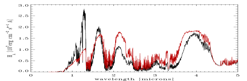
Figure 8: Predicted emergent flux for the models displayed in Fig. 6. Black line: cloudless model; gray line (red in the online version): cloudy model.

Another possible numerical trick is a “rezoning” of depth points. It was found that it is more accurate and numerically mode stable to add several depth points at the newly determined low-pressure base of the cloud deck and immediately above it. Otherwise, if there are too few depth points in the region of exponential decline of the cloud-shape function on the low-pressure side of the main cloud, the opacity of the cloud would be overestimated. Analogously, if there is no depth point exactly at the cloud base, the opacity of the cloud is underestimated.

Some results that illustrate an influence of clouds are shown in Figs. 5 – 8. We compare a cloudless model considered earlier with $T_{\rm eff}$ = 1500 K, $\log g=5$, to an analogous model with an added forsterite (Mg₂SiO₄) cloud. The low (high-pressure) cloud boundary is set at a fixed temperature of $T=2300$ K that simulates an effect of a whole set of other magnesium silicate condensates, as suggested by Burrows et al. (2006). Notice that even if the lower cloud boundary is specified at a fixed temperature, it is not fixed in the physical space because the temperature structure varies from iteration to iteration. The upper (low-pressure) cloud boundary is set exactly at the intersection of the $T-P$ profile and the forsterite condensation curve. The power-law cloud shape parameters defined by Eq. (2.63) are set to $c_{0}=2$ and $c_{1}=10$. The modal particle size is taken to be 100 microns.

Figure 5 displays the convergence pattern of a model with clouds, computed using the Rybicki scheme. As is clearly seen, the convergence is again quite fast a very stable; the whole computation took about 30 s on the same MacBook Pro laptop as mentioned in § 3.3. Figure 6 shows the temperature structure, displayed as the temperature as a function of Rosseland optical depth for both, cloudless and cloudy models. Differences in the temperature structure are clearly seen.

The effects of the cloud are best seen on a plot of the total radiative and convective energy flux, displayed in in Fig. 7. The upper panel shows the cloudless model, which exhibits a smooth rise of $F^{\rm conv}/(\sigma_{\!R}T_{\rm eff}^{4})$ toward deep layers, starting around $\tau_{\rm ross}\approx 1$. From the numerical point of view, notice that the total flux is conserved within about 0.05%; this is not seen on this plot but is shown later in Fig. 10. The lower panel represents an analogous plot for the cloudy model, together with the cloud shape function. The later plot clearly shows that the cloud contributes to the total opacity at Rosseland optical depths roughly between 1 and 10. Because of an additional opacity as compared to the cloudless model, the temperature gradient is flatter in this region, and consequently the radiative flux is somewhat lower. The relative portion of the convective flux in this region thus somewhat increases. In contrast, in the region just below the cloud, the temperature gradient increases and so does the radiative flux, and consequently the portion of the convective flux decreases dramatically.

Finally, we show in Fig. 8 the predicted emergent flux for both models. The main effect of clouds is to fill the opacity windows at 1.2 and 1.6 microns where the cloudless model exhibits the highest peaks of the spectral energy distribution. By virtue of the radiative equilibrium, this energy has to be redistributed in other spectral regions, and therefore the flux increases essentially everywhere for wavelengths larger than about 1.8 microns.

5.3 Global formal solution

The term “global formal solution” refers to the set of all calculations between two iterations of the overall iteration (i.e., linearization) scheme.

The main part of this procedure is a solution of the radiative transfer equation for specific intensities and an evaluation of the Eddington factors, as described above in § 4.

In parallel with, or on top of, this procedure, one performs other “formal” solutions, essentially updating one state parameter by solving the appropriate equation, while keeping other state parameters fixed. For instance, and most importantly, one solves the radiative/convective equilibrium equation to update temperature in the convection zone and below it. To this end, several procedures were devised for convective models to iteratively improve the $T$-$P$ profile before entering the next linearization step. In most cases, using such procedures has very favorable consequences for the convergence properties, or even prevents an otherwise violent divergence of the iteration scheme. These procedures will be described next in § 5.4.

For models with clouds, one then determines the new positions of the cloud bases as described in § 5.2. This changes the opacity as a function of depth, so one has to perform another formal solution of the radiative transfer equation, as well as the radiative/convective equilibrium, and the whole procedure may be iterated several times.

5.4 Correction of temperature in the convection zone

Although the linearization scheme may in principle converge without additional correction procedures, in practice it is a rare situation. The essential point is that a linearization iteration may yield current values of temperature and other state parameters such that, for instance, the actual logarithmic gradient of temperature in a previously convective region may spuriously decrease below the adiabatic gradient at certain depth points. Consequently, these points would be considered as convectively stable, and in the next iteration the radiative flux would be forced to be equal to the total flux. This would lead to a serious destabilization of the overall scheme, likely ending in a fatal divergence.

It is therefore often necessary to perform certain correction procedures to assure that the convection zone is not disturbed by spurious non-convective regions, and analogously the radiative zone is not disturbed by spurious convective region, so that the temperature and other state parameters are smooth functions of depth before one enters the next iteration of the overall linearization scheme. We describe these schemes below.

5.4.1 Improved definition of convection zone

. After a completed linearization iteration, one examines the depth points in which the actual temperature gradient surpasses the adiabatic one. If such a point is solitary, or if it occurs at much lower pressures than the upper boundary of the convection zone in the previous iteration, the point is declared as convectively stable, and the usual radiative equilibrium equation is solved for it in the next iteration step.

On the other hand, if there is/are depth points in which $\nabla<\nabla_{\rm ad}$ (so that they are seemingly convectively stable), surrounded on both sides by points that are convectively unstable, $\nabla\geq\nabla_{\rm ad}$, these points are declared as convectively unstable, and are considered to be part of the convection zone. In such a newly defined convection zone, one or both of the following correction procedures are performed.

5.4.2 Standard correction procedure

. The idea of the correction is as follows. In view of eq. (2.34), the convective flux is given by

$$F_{\rm conv}=F_{0}(\nabla-\nabla_{\rm el})^{3/2},$$ (5.1)

where

$$F_{0}=(gQH_{P}/32)^{1/2}(\rho c_{P}T)(\ell/H_{P})^{2}.$$ (5.2)

After a completed iteration of the global linearization scheme, one takes the current values of the state parameters and the radiation flux, and computes, in the convection zone, the new convective flux corresponding to this radiation flux so that the total flux is perfectly conserved,

$$F_{\rm conv}^{\ast}=F_{\rm tot}-F_{\rm rad},$$ (5.3)

where $F_{\rm tot}=\sigma_{\!R}T_{\rm eff}^{4}$. If $F_{\rm rad}$ is spuriously larger than $F_{\rm tot}$, then $F_{\rm rad}$ is set to $0.999F_{\rm tot}$. The new difference of the temperature gradients corresponding to this convective flux is then

$$\nabla-\nabla_{\rm el}=(F_{\rm conv}^{\ast}/F_{0})^{2/3},$$ (5.4)

which is related to $\nabla-\nabla_{\rm ad}$ through

$$\nabla-\nabla_{\rm ad}=(\nabla-\nabla_{\rm el})+B\sqrt{\nabla-\nabla_{\rm el}}.$$ (5.5)

where $B$ is given by eq. (2.36). Both $B$ and $\nabla_{\rm ad}$ are computed using the current values of the state parameters. Equation (5.5) thus yields the new gradient $\nabla$ and, with the pressure being fixed, the new temperature. With the new temperature, one recalculates the thermodynamic variables, and iterates the process defined by equations (5.2) - (5.5) to convergence.

In solving eq. (5.5), one proceeds from the top of the convection zone to the bottom, because the gradient $\nabla$ is numerically given by

$$\nabla_{d}\equiv\nabla_{d-1/2}=\frac{T_{d}-T_{d-1}}{P_{d}-P_{d-1}}\frac{P_{d}+P_{d-1}}{T_{d}+T_{d-1}}.$$ (5.6)

or by

$$\nabla_{d}=\ln(T_{d}/T_{d-1})/\ln(P_{d}/P_{d-1}),$$ (5.7)

so in order to evaluate $T_{d}$ one needs to know $T_{d-1}$ in the previous depth point.

5.4.3 Refined correction procedure

The above procedure is improved by recognizing that the coefficient $B$ is an explicit function of temperature, so $B$ can be expressed as $B\equiv\beta T^{3}$. More importantly, the radiation flux is not kept fixed, but is written as

$$F_{\rm rad}\equiv\alpha T^{4}\nabla,$$ (5.8)

so that instead of keeping $F_{\rm rad}$ fixed, one first computes $\alpha$ from (5.8) for the current values of $T$ and $\nabla$, and rewrites combined equations (5.3) –(5.5) as a non-linear equation for temperature,

$$\nabla(T)=\nabla_{\rm ad}+\left(\frac{F_{\rm tot}-\alpha T^{4}\nabla(T)}{F_{0}}\right)^{2/3}+\beta T^{3}\left(\frac{F_{\rm tot}-\alpha T^{4}\nabla(T)}{F_{0}}\right)^{1/3},$$ (5.9)

where the parameters $\alpha$ and $\beta$ are held fixed. Equation (5.9) is solved by the Newton-Raphson method, again going from the top of the convection zone to the bottom.

These procedures were developed by Hubeny & Burrows (2007), but not explicitly described there. Experience showed that they may be very helpful, but should be used judiciously. The best strategy is to start using them around the third or fourth iteration of the linearization scheme (otherwise, the radiation flux is so far from the correct value that the correction cannot work properly), and to stop using them at some later (e.g., 15th) global iteration. The reason for this cutoff is that an application of the refinement procedures for an almost converged model may lead to an oscillatory behavior of the temperature corrections, in the sense that the refinement procedures change the temperature slightly, while the subsequent linearization iteration changes it back.

6 Gray and pseudo-gray models

It is instructive to consider the so-called gray, or pseudo-gray models. These are approximate models, but they serve two purposes: (i) they can be used as initial models for the linearization scheme, and (ii) they can provide a valuable physical insight into the properties of the computed atmospheric structure.

They are based on the two moment equations of the transfer equation, Eqs (2.13) and (2.14), rewritten to contain derivatives with respect to the column mass $m$, and integrated over frequencies, namely

$$\frac{dH}{dm} = \kappa_{J}J-\kappa_{B}B,$$ (6.1)

$$\frac{dK}{dm} = \chi_{\!H}H,$$ (6.2)

where

$$[J,H,K]\equiv\int_{0}^{\infty}[J_{\nu},H_{\nu},K_{\nu}]\,d\nu$$ (6.3)

are the frequency-integrated moments of the specific intensity, and

$$\kappa_{J} \equiv \int_{0}^{\infty}\!\!(\kappa_{\nu}/\rho)J_{\nu}d\nu/J,$$ (6.4)

$$\kappa_{B} \equiv \int_{0}^{\infty}\!\!(\kappa_{\nu}/\rho)B_{\nu}d\nu/B,$$ (6.5)

$$\chi_{\!H} \equiv \int_{0}^{\infty}\!\!(\chi_{\nu}/\rho)H_{\nu}d\nu/H,$$ (6.6)

are the absorption mean, the Planck mean, and the flux-mean opacities, respectively. Here

$$B\equiv\int_{0}^{\infty}\!\!B_{\nu}d\nu=(\sigma_{\!R}/\pi)T^{4},$$ (6.7)

is the frequency-integrated Planck function, which is proportional to $T^{4}$. As is customary, the mean opacities are defined using the monochromatic opacities per gram. Notice that $\kappa_{J}$ and $\kappa_{B}$ are defined through the true absorption coefficient (without scattering), while $\chi_{\!H}$ is defined through the total absorption (extinction) coefficient.

Assuming radiative equilibrium, $dH/dm=0$, Eq. (6.1) reduces to

$$\kappa_{J}J=\kappa_{B}B,\quad{\rm or}\quad B=(\kappa_{J}/\kappa_{B})J,$$ (6.8)

which shows that the temperature structure is given through the ratio of the absorption mean to the Planck mean opacities, and the integrated mean intensity, which is given by the solution of the transfer equation. From the second moment equation we have

$$K(\tau_{H})=H\tau_{H}+K(0)=(\sigma_{\!R}/4\pi)T_{\rm eff}^{4}\tau_{H}+K(0),$$ (6.9)

where $d\tau_{H}=\chi_{\!H}dm$ is the optical depth associated with the flux-mean opacity. We express the moment $K$ through $J$ via an integrated Eddington factor, $f_{K}\equiv K/J$, and using an integrated second Eddington factor, $f_{H}\equiv H(0)/J(0)$, Eq. (6.8) together with (6.9) gives (see also Hubeny et al. 2003)

$$T^{4}=\frac{\kappa_{J}}{\kappa_{B}}\left[\frac{3}{4}T_{\rm eff}^{4}\left(\frac{1}{3f_{K}}\tau_{H}+\frac{1}{3f_{H}}\right)+\frac{\pi}{\sigma_{\!R}}H^{\rm ext}\right].$$ (6.10)

This expression is exact, but is only formal because $\kappa_{J}$, $f_{K}$, $f_{H}$, and $\tau_{H}$ are not a priori known. However, this expression is very useful if one makes some additional approximations.

Classical gray model without irradiation. It assumes that the opacity is independent of frequency. In this case one has an exact mathematical solution,

$$T^{4}=\frac{3}{4}\,T_{\rm eff}^{4}\,[\tau+q(\tau)],$$ (6.11)

where $q(\tau)$ is the Hopf function, a monotonically varying function between $q(0)=1/\sqrt{3}\approx 0.577$ and $q(\infty)\approx 0.71$. Temperature structure given by (6.11) is exact for a truly frequency-independent (gray) opacity, but it can be used as a useful starting approximation for any opacity, provided that $\tau$ is presented by a properly chosen mean opacity. As follows from the general expression (6.10), the appropriate opacity should be an approximation of the flux mean opacity. It turns out that such an approximation is the Rosseland mean opacity. Specifically, in the deep layers where the diffusion approximation applies,

$$H_{\nu}\approx\frac{1}{3}\frac{dB_{\nu}}{d\tau_{\nu}}=\frac{1}{3}\frac{dB_{\nu}}{(\chi_{\nu}/\rho)dm}=\frac{1}{3}\frac{1}{(\chi_{\nu}/\rho)}\frac{dB_{\nu}}{dT}\frac{dT}{dm},$$ (6.12)

and therefore

$$\chi_{\!H}=\frac{\int_{0}^{\infty}\!\!(\chi_{\nu}/\rho)H_{\nu}d\nu}{\int_{0}^{\infty}\!\!H_{\nu}d\nu}\approx\frac{\int_{0}^{\infty}(dB_{\nu}/dT)\,d\nu}{\int_{0}^{\infty}[1/(\chi_{\nu}/\rho)](dB_{\nu}/dT)\,d\nu}\equiv\chi_{\!R},$$ (6.13)

where the second equality is the definition of the Rosseland opacity.

Gray model with Eddington approximation. In our notation, the Eddington approximation sets $f_{K}=1/3$ and $f_{H}=1/2$, and the Hopf function is taken as constant, $q(\tau)=2/3$. Equation (6.11) still applies.

Eddington approximation, but allowing for non-gray opacity. In this case, the temperature structure is

$$T^{4}=\frac{\kappa_{J}}{\kappa_{B}}\left(\frac{3}{4}\,T_{\rm eff}^{4}\big{[}\tau+2/3\big{]}\right).$$ (6.14)

Eddington approximation, with non-gray opacity, and with external irradiation.

$$T^{4}=\frac{\kappa_{J}}{\kappa_{B}}\left(\frac{3}{4}\,T_{\rm eff}^{4}\big{[}\tau_{H}+2/3\big{]}+WT_{\ast}^{4}\right),$$ (6.15)

where the external irradiation flux is expressed through the effective temperature of the irradiating star, $T_{\ast}$, and the dilution factor, $W$, given by Eq. (2.52). As shown by Hubeny et al. (2003), this expression helps to understand a possible temperature rise at the surface of strongly irradiated planets,, and even the fact that under certain circumstances one can obtain two legitimate solutions of the structural equations – one for the temperature monotonically decreasing outward, and one exhibiting a temperature rise toward the surface.

Mathematically speaking, these effects arise due to an inequality of the absorption mean and the Planck mean opacities in the surface layers, namely that $\kappa_{J}/\kappa_{B}$ may become significantly larger than unity. The reason for this is that the Planck mean opacity weighs the monochromatic opacity by $B_{\nu}(T)$, the Planck function at the local temperature, while $\kappa_{J}$ close to the surface weighs the monochromatic opacity by $B_{\nu}(T_{\ast})$, the Planck function at the effective temperature of the irradiating star, $T_{\ast}$, which is significantly larger than $T$. If, in addition, one has a strong opacity source acting in the optical region (where the stellar irradiation has the maximum), one can easily obtain $\kappa_{J}/\kappa_{B}\gg 1$ close to the surface. Further from the surface, where less incoming radiation penetrates, $\kappa_{J}\rightarrow\kappa_{B}$, which leads to a decrease of the local $T$ as compared to the surface value. A more comprehensive discussion is presented in Hubeny et al. (2003) and Hubeny & Mihalas (2014; § 17.7).

Two-step gray models. A variant of the above approaches is a two-step gray model, which divides the whole frequency range into two regions, typically a "visible" and an "infrared", one, and assumes a frequency independent opacity $\chi_{\rm vis}$ and $\chi_{I\!R}$, with $\chi_{\rm vis}\not=\chi_{I\!R}$, and analogously for $\kappa$ and the scattering coefficient $s$. In the two regions one typically invokes different approximations. Such models were developed by Hansen (2008), Guillot (2010) and Parmentier & Guillot (2014).

We will not discuss this topic any further because our emphasis here is on constructing model atmospheres without any unnecessary approximations. We use gray or pseudo-gray models just as am initial estimate for subsequent iterative procedure, or as a pedagogical tool to understand the atmospheric temperature structure.

7 Comparison to available modeling approaches and codes

Here we briefly describe various modeling approaches and codes used in the literature and compare them to the formalism described above. We stress that we will consider here only the codes and approaches that aim at determining a self-consistent atmospheric structure, obtained by a simultaneous solution of the basic structural equations summarized in Section 2, or at least a temperature structure that is consistent with the radiation filed. We will not consider here approaches that employ for instance an ad hoc, or parametrized, temperature structure and solve just for the radiation field, or using an approximately described, fixed radiation field to determine the atmospheric structure.

Therefore, in the exoplanet terminology, we will consider here only the forward, self-consistent codes, but we will not consider the retrieval codes, such as the code of Madhusudhan & Seager (2009, 2011), NEMESIS (Irwin et al. 2008; Barstow et al. 2017), CHIMERA (Line et al., 2012, 2013), or Tau-REX (Waldmann et al., 2015), to name just a few.

From the basic physical point of view, we will limit ourselves here to hydrostatic, plane-parallel models, because considering more sophisticated multi-dimensional dynamical models is a different topic that requires different computational strategies.

7.1 Philosophy

Modeling atmospheres of substellar-mass objects is obviously a young field, whose beginnings occurred in the mid and late 1990’s, shortly after observational discoveries of these objects. In an endeavor to provide a needed theoretical background, it was deemed most straightforward to adapt some already available modeling approaches and codes to the physical conditions expected to occur in SMO atmospheres. There were two avenues taken in this regard: (i) adapting modeling codes for stellar atmospheres, and (ii) adapting codes developed for modeling solar system planets and moons. Both avenues offer certain advantages and certain challenges, as we will outline below. Only recently, there appear new codes which were developed from the scratch, and which may potentially offer a possibility of avoiding drawbacks and biases inherent in adapting existing codes.

We shall briefly discuss the most popular and widely used codes in these three categories. We stress that this is not meant as a comprehensive review of the subject, but rather as a brief guide to understand what is involved, from both physical and numerical point of view, in the present most popular modeling codes.

7.2 Adapting stellar atmosphere codes

The first category of codes are those that were created by adapting a code for computing model stellar atmospheres. It should be pointed out that computing model stellar atmospheres is a very mature subject, having been developing during the last almost seven decades. Even the state-of-the-art NLTE metal-line blanketed models are around for over two decades. The stakes in the stellar atmospheres theory are also very high thanks to an unprecedented quality and quantity of high-resolution, high signal-to-noise spectroscopic observations that put heavy demands of the accuracy and reliability of theoretical analysis tools.

It is therefore quite natural to model atmospheres of SMOs by adapting existing stellar atmospheres codes. There are specific features that make computing SMO model atmospheres easier that computing model stellar atmospheres, and vice versa. We will briefly summarize them below.

The features that make the SMO models easier to compute are:

1. In stellar atmospheres, in particular for hot stars, the hydrostatic equilibrium equation contains a contribution of radiation pressure, which involves an additional coupling of the gas pressure (and therefore the mass density) to the radiation field.

2. For both types of objects, the opacity varies rapidly with frequency. However, for stars, the (mostly) atomic lines are distributed randomly in frequency, while for SMOs, the (mostly) molecular lines tend to be organized in bands, which makes it more suitable to employ various statistical techniques such as the opacity distribution functions, or, as they are called in the planetary community, the correlated $k$-coefficients. Also, for stars, there are no frequency regions that can be treated as purely (or mostly) scattering or purely (or mostly) absorbing.

3. These two issues play a role already in LTE models. For NLTE models, a major difficulty comes from the fact that the opacities and emissivities depend on the populations of levels involved in the corresponding atomic transitions, which in turn depend on the radiation field via the kinetic equilibrium equation. The opacities thus cannot be evaluated a priori as functions of temperature and density, but have to be computed self-consistently with all the structural equations. There are typically thousands to tens of thousands atomic energy levels involved in the atomic transition (lines or continua) that make a significant contribution to the total opacity. Although in the field of SMO model atmosphere, there are studies that consider NLTE effects (e.g., Fortney et al. 2004), stellar atmosphere models consider NLTE on much larger scale. For instance, in a grid of model atmospheres of B stars (Lanz & Hubeny 2007), one considers about 1130 energy levels and about 39,000 lines of light elements, and 500,000 to 2 million lines dynamically selected from a list of about 5.6 million lines of the iron peak elements, in full NLTE.

All these complications are absent or alleviated for models of SMO’s. Modifying a modern NLTE stellar atmosphere code thus mostly involves removing many routines dealing with special issues of NLTE (an evaluation of transition rates, solving the kinetic equilibrium equation, etc.), and evaluating opacities and emissivities on the fly, because in any LTE model atmosphere code, including that for SMO’s, it is much more efficient to use pre-calculated opacity tables.

On the other hand, computing SMO model atmospheres is more difficult than computing model stellar atmosphere, particularly for hot stars. We stress that at the cool end of the main sequence, K and M stars, one meets most of the challenges listed below for SMO’s.

1. One has to include a solution of chemical networks to determine the concentrations of the individual molecular species as functions of temperature and pressure. However, this is not difficult numerically or algorithmically; the difficulty is mostly in finding appropriate molecular data. In any case, this can be done independently of a model construction.

2. As pointed out above, more sophisticated models needs to consider departures from chemical equilibrium.

3. One has to add a treatment of cloud formation, together with an evaluation of cloud absorption and scattering. This is perhaps the most difficult part of the process of adapting approaches and codes designed for hotter objects, because it involves basic physical problems (e.g., determining consistent particle sizes, their distribution, and a position of a cloud in the atmospheres), as well as algorithmic and numerical problems in incorporating these effect in a self-consistent manner.

4. Although not as serious as other problems listed above, the presence of strong (and generally anisotropic) external irradiation brings challenges on adopted numerical schemes, in particular for self-consistent models.

Here is a list of the codes that were created by adapting their stellar atmospheric counterpart.

7.2.1 CoolTLUSTY

This code is a variant of a general stellar atmosphere (and accretion disk) code tlusty, originally described in Hubeny (1988) and Hubeny & Lanz (1995). Its modification for SMO atmospheres, called CoolTlusty was briefly described in Sudarsky et al. (2003) and Hubeny et al. (2003).

The present paper in fact describes in more detail the physical and numerical background of CoolTlusty. The input atomic and molecular physics and chemistry is quite flexible. It can either use opacity tables generated using the Burrows & Sharp (1999) and Sharp & Burrows (2007) approach, or any other opacity tables, both for the total opacity, as well as a set of tables for individual species. The input properties of condensates (cloud absorption and scattering) can accept any tables generated by a Mie code. Originally, it was using tables generated as described in Sudarsky et al. (2000); recently it switched to tables generated by Budaj et al. (2014).

7.2.2 PHOENIX

Code PHOENIX was developed for stellar or even supernova applications, see Hauschildt & Baron (1999). The first application for extrasolar giant planets was done by Barman et al. (2001). The input physics is analogous to that used in CooTtlusty, described above. The basic difference is the adopted numerical scheme; PHOENIX is using a different flavor of the ALI method. It also uses a different set of chemical/molecular data, and a different treatment fo clouds.

7.2.3 UMA

UMA stands for Upsalla Model Atmospheres code (Gustafsson et al. 1974), somewhat modified by Vaz & Nordlund (1985). It was further adapted to studies of extrasolar giant planets by Seager & Sasselow (1998), see also Seager & Sasselow (2000), and Seager et al. (2000). It does not use an ALI scheme; it solves the radiative transfer equation by the Feautrier method, and determines the temperature structure self-consistently with the radiation field by a classical temperature correction.

7.3 Adapting planetary atmosphere codes

Generally, the codes of this category are directly based on approaches used originally for atmospheres of the solar-system planets or moons. Some, but not all, are based on, or use the spirit of, approaches used originally for the Earth atmosphere. After the observational detections of brown dwarfs and extrasolar giant planets in the mid and late 1990’s and early 2000’s, some of these codes were adapted to these objects.

In the Earth atmosphere there is a clear distinction between the two following wavelength regions:

1. The optical wavelength region (often called “solar frequencies”), which is optically thin in most of the visible wavelengths, and the transport of radiation is dominated by the scattering processes; and

2. The infrared region, where the radiation transport is dominated by absorption and thermal emission. It should be noted that the atmosphere is opaque in the short-wavelength regions (UV and X-ray), but these regions are inconsequential for constructing structural models.

The original Earth-atmosphere codes used that distinction explicitly to develop suitable approximations of the radiative transfer equation that differ in the optical and the infrared region. The early codes for modeling solar-system planets often used at least some aspects of this distinction. However, when applying such a dichotomous model to significantly hotter or otherwise quite different conditions in the exoplanets and brown dwarfs, these procedures may become less accurate or less efficient than those based on the formalism outlined above.

While the existing codes of this category do still yield valuable results, the above considerations should be kept in mind when developing new codes for modeling atmospheres of extrasolar planets of brown dwarfs. Figuratively speaking, it seems more efficient to treat exoplanets and brown dwarfs as small and cool stars rather than hot and big Earths’ or solar system planets.

7.3.1 McKay-Marley code

The code was first developed by McKay et al. (1989) for calculating atmospheric structure and spectra of Titan, and subsequently extended and applied for atmospheres of brown dwarfs by Marley et al. (1996); Burrows et al. (1997), to the solar-system giant planets by Marley & McKay (1999), and applied for atmospheres of exoplanets by Marley et al. (1999), Fortney et al. (2005, 2008), and subsequently in a large number of SMO studies.

Here we list the main assumptions and approaches used by the code, stressing the differences form the approach described in this paper and/or used in the above mentioned codes.

The code determines the $T$-$P$ profile in the following way: In the convection zone (or possibly multiple zones) the temperature gradient is assumed to be strictly adiabatic, and all the flux is transported solely by convection. In the radiative zone, where the strict radiative equilibrium applies, one employs a special temperature-correction procedure, which somewhat resembles the Rybicki scheme described above, in the sense that one forms a vector of the local temperatures, ${\bf T}\equiv\{T_{1},\ldots,T_{N\!R}\}$, where $N\!R$ is the number of depth points in the radiative zone, and computes a correction $\delta{\bf T}$ by using the following matrix equation (in our notation)

$${\bf A}\,\delta{\bf T}=\sigma_{\!R}T_{\rm eff}^{4}-{\bf F}({\bf T}_{0}),$$ (7.1)

where ${\bf F}({\bf T}_{0})$ is a vector of the total radiative flux in all the depth points of the radiative zone, computed for the current vector of temperatures, ${\bf T}_{0}$.. Equation (7.1) in fact represents a linearization, or a Newton-Raphson solution, of a non-linear implicit relation between the radiative flux and the temperature, ${\bf F}({\bf T})=\sigma_{\!R}T_{\rm eff}^{4}$, expressing the constancy of the total radiative flux. Matrix ${\bf A}$ is the corresponding Jacoby matrix, $A_{ij}=\partial F_{i}/\partial T_{j}$; that is, the $ij$-component of ${\bf A}$ expresses the response of the total flux at depth $i$ to the temperature at depth $j$. Unlike the Rybicki scheme, the elements of the Jacoby matrix are not evaluated analytically. Instead, they are obtained by solving a set of additional radiative transfer equations, by consecutively modifying a single component of vector ${\bf T}$, for instance $T_{j}\rightarrow T_{j}+\Delta T$ (with $\Delta T$ having a small, arbitrary value such as 1 K), while keeping the other components unchanged, to obtain a perturbed flux at all depth points, ${\bf F}^{p,j}$. The elements of the Jacoby matrix are then set to

$$A_{ij}=(F_{i}^{p,j}-F_{i})/\Delta T.$$ (7.2)

Radiative transfer equation is solved by a variant of the two-stream approximation, called two-stream source function method (Toon et al. 1989). It considers an atmosphere composed of a set of zones, and assumes that the thermal source function (i.e., the Planck function) is a linear function of optical depth within a given zone. The method essentially solves the first moment equation of the radiative transfer equation directly for the radiative flux, where some empirical relation between the zero-order moment (mean intensity) and the first-order moment (flux) is invoked. This scheme improves the traditional two-stream methods in situations where scattering is present, by considering the scattering source function computed using the proper phase functions, but using the specific intensities obtained from the traditional two-stream approximation for the thermal radiation.

The line opacity is treated using a variant of the Opacity Distribution Function approach (see § 5.1), called here the $k$-coefficient method. The opacity is assumed to be constant within a given depth zone, which allows one to introduce a $k$-coefficient not as a true opacity distribution function, as is done in the stellar context, but directly as a distribution of the transmission coefficients.

In conclusion, the adopted method for solving the transfer equation is inherently approximate and only first-order accurate, in contrast to the Feautrier scheme or DFE used in the above approaches, which are second-order accurate (i.e., a numerical solution of the transfer equation is exact for a piecewise parabolic source function). However, this is usually not a big concern or a source of inaccuracies of the resulting model.

A potentially more serious source of inaccuracies lies in the treatment of radiative equilibrium. While the temperature correction expressed by Eq. (7.1) correctly takes into account the fact that a local flux is determined by the global temperature structure, an evaluation of the elements of the Jacobian numerically by differencing two numerical solutions, moreover approximate ones, of the transfer equation, may lead to inaccuracies, in particular in optically thin regions.

Even more seriously, the radiative equilibrium constraint is applied solely for the flux, and only the condition $\int\!F_{\nu}d\nu={\rm const}$ is checked. A fulfillment of this condition is viewed as a verification that a model is well converged for the $T$-$P$ profile. However, experience gained from constructing model stellar atmospheres revealed that at the upper, optically thin portion of the atmosphere, the radiation flux is quite insensitive to the local temperature, because it is essentially fixed by the source function at the monochromatic optical depth around 2/3. The temperature structure in the upper layers may thus remain quite inaccurate even if the total flux is conserved within, say, 1% or even less. As discussed above, what is needed in upper layers is to employ the integral form of the radiative equilibrium, $\int\kappa_{\nu}(B_{\nu}-J_{\nu})d\nu=0$, which does not seem to be done in this approach.

Figure 9: Temperature structure for the radiative zone of a brown dwarf model with with $T_{\rm eff}=1500$ K, $\log g=5$, considered in § 3.3 – full line, and an artificially perturbed model – crosses.

Figure 10: Upper panel: relative difference (in per cents) of the computed radiative and the nominal flux, $\sigma_{\!R}T_{\rm eff}^{4}$ for the models displayed in Fig. 9. Full line represents the original model, while the diamonds represent the perturbed model. Dotted line corresponds to the exact flux with the relative difference equal to zero. Lower panel: the net relative cooling rate for the same models. Here the crosses represent the exact model. Notice that while the total radiative flux for the perturbed model as still accurate within about 1%, the net relative cooling exhibits huge differences from the exact model, reaching about 120%.

To demonstrate these considerations numerically, we take a brown dwarf model with $T_{\rm eff}=1500$ K, $\log g=5$, considered in § 3.3, and perturb artificially the temperature structure in the upper layers by adding a damped wavy pattern with an amplitude $0.3$ times the actual temperature – see Fig. 9. For this model we recompute the radiative flux, and the heating/cooling rates. Figure 10 shows the flux and the heating/cooling rates. While the computed radiation flux differs at most by 1% (close to the column mass $m\approx 1$ g cm${}^{{}_{2}}$), and therefore such model could have easily been declared as reasonably converged, the net cooling rate, $\int\kappa_{\nu}(B_{\nu}-J_{\nu})\,d\nu\Big{/}\int\kappa_{\nu}B_{\nu}d\nu$ shows significant differences from zero. This illustrates the above stated warning that in order to assess an accuracy of the model, one needs to check not only a conservation of the total flux, but also an equality of the heating and cooling rates as stipulated by the constraint of the radiative equilibrium.

However, we stress that while the above analysis demonstrates that the McKay-Marley temperature correction scheme may lead to an inaccurate determination of the temperature in the upper layers of an atmosphere, it did not prove that the results are necessarily inaccurate. Moreover, even if inaccuracies occur, they are likely limited to the optically layers, which in turn have relatively little influence on the predicted emergent radiation.

7.3.2 Goukenleuque et al.’s code

Goukenleuque et al. (2000) presented one of the first self-consistent model atmospheres of an extrasolar giant planet, 51 Peg b in this case. To our knowledge, this code was not used very much after this study. It takes into account cloud opacity and scattering, but on the other hand completely neglects convection, which represents a significant drawback. Radiative transfer equation is solved approximately, using a variant of the two-stream method with Eddington approximation. The code iterates between solving the transfer equation, and subsequently correcting temperature by solving the radiative equilibrium equation.

One invokes two nested iteration loops. In the inner loop one holds the chemical composition, cloud position, and the opacities fixed at the current values, and determines the temperature that gives the correct total flux. The outer loop takes the $T$-$P$ profile determined in the inner loop, and computes new chemical equilibrium composition and new opacities corresponding to this $T$-$P$ profile. The authors mention that some 1000 (!) iterations were needed in the inner loop, which, when compared to the linearization scheme outlined above that requires some 10 - 20 iterations, clearly demonstrates a relative inefficiency of this and other similar schemes that do not solve all the structural equations simultaneously.

7.4 Independent, newly developed codes

7.4.1 PETIT

The code is described in detail by Mollière et al. (2015). Although we list the code as newly developed, the radiative transfer solver and the method of the solution of the radiative equilibrium equation were developed already by Dullemond et al. (2002), and used in a code for computing vertical structure of massive circumstellar disks.

Code PETIT solves the radiative equilibrium and chemical equilibrium equations together with the radiative transfer equation using a specific application of the variable Eddington factor technique. Molecular line opacity is treated using the correlated $k$-coefficient method. The radiative equilibrium equation is considered in a form analogous to our Eq. (6.10), where the Planck mean and the absorption mean opacities, together with the Eddington factors, are determined iteratively by solving the radiative transfer equation frequency by frequency. In the convectively unstable layers, the temperature gradient is taken to be adiabatic, and the integrated mean intensity of radiation is taken as a scaled integrated Planck function. External irradiation is treated by a variant of the two-stream approximation.

Other approximation is that the PETIT code neglects any scattering process in the transfer equation (see Appendix C1 of Mollière et al. 2015). Also, although the chemical equilibrium calculations contain some condensed species, cloud formation and opacity is not considered, which limits the general applicability of the code.

7.4.2 GENESIS

The code, together with its first actual applications, is described in detail in Gandhi & Madhusuhan (2017). It essentially uses the structural equations and the numerical procedures described in this paper, namely the linearization method with the Rybicki reorganization scheme to solve the coupled radiative transfer together with the radiative/convective equilibrium equation, and the Feautrier method for the formal solution of the transfer equation. Convection is treated using the mixing-length formalism, analogously as described here. In the present version, the code does not consider cloud opacity and scattering.

7.4.3 HELIOS

The code and its benchmark tests are described in a recent paper (Malik et al. 2017) Although the code is newly developed from the scratch, it keeps using approximate and thus potentially inaccurate approaches and numerical schemes, having their origin in an old Earth/planetary-type philosophy of atmospheric modeling, briefly discussed above. Here is a list of some shortcomings of the adopted procedure:

1. The radiative transfer equation is solved by a variant of the two-stream approximation which uses an analytic solution for the individual layers, assuming either isothermal structure inside a layer, or a linearly varying Planck function within a layer. The latter still yields only a first-order accurate numerical scheme. Although a solution for one layer is obtained analytically, the final solution of the transfer equation for all layers still requires a numerical procedure. Relative complexity of the proposed algorithm, which is still approximate, contrasts with the procedure outlined above which yields an “exact” numerical solution, for physical problems of varying complexity, in a very simple and transparent way.

2. From the paper (Malik et al. 2017) it appears that the scheme does not include convection at all. If this is indeed so, it is a significant drawback which seriously limits an applicability of the code.

3. Analogously, the published description does not contain any mention of the cloud opacity and scattering. Such a limitation is however present in other codes mentioned here.

4. In any case, regardless of the deficiencies expressed in (ii) and (iii), the radiative equilibrium constraint is treated as a some sort of time-dependent approach to equilibrium. While this is in principle acceptable, the whole procedure still represents an iterative scheme alternating between (an approximate) solution of the transfer equation with fixed temperature and a solution (again approximate) of the radiative equilibrium equation. Experience gained from computing model stellar atmospheres revealed that this procedure may converge very slowly, or may even suffer from the problems of false convergence (i.e., relative changes may become small, but the current solution is still far from the correct one – see, e.g. Hubeny & Mihalas (2014; § 13.2). Furthermore, their formulation of the radiative equilibrium equation uses thermodynamic parameters such as specific heat $c_{P}$, and thus ignores the microphysics of the interaction of radiation and matter, as contained e.g. in Eq. (2.25).

8 Conclusions

The aim of this paper was to summarize current physical, mathematical, and numerical methodology for computing model atmospheres of substellar mass objects within a framework of plane-parallel, static models. These two basic assumptions make the problem tractable on present-day computers. The remaining uncertainties and problems are not of an algorithmical or computational nature, but rather are caused by the lack of data from other branches of physics and chemistry – in particular, data for molecular lines, details of line broadening, formation and detailed properties of condensed particles, and the rates of chemical reactions for treating non-equilibrium chemistry, to name just few of the most pressing problems.

Our basic philosophy is the following. While we acknowledge the existence of many problems and uncertainties that plague our description of the SMO atmospheres, we feel that the physical formulation and corresponding mathematical treatment of phenomena that are currently well understood has to be done accurately, reliably, and without unnecessary approximations and simplifications.

For instance, a treatment of an interaction of radiation and matter, moreover in a highly non-equilibrium conditions, has been developed to a high degree of sophistication in stellar astrophysics; for a recent summary, see, e.g, Hubeny & Mihalas (2014). Also, many efficient and fast numerical algorithms were developed in the last two decades. Yet, many approaches and numerical codes used for modeling SMO atmospheres are still unnecessarily based on old and outdated methodologies. In our opinion, this is caused, at least in part, by the lack of proper communication between researchers in the fields of planetary and stellar atmospheres. Another reason is the fact that in the present period of a rapid development of the field of exoplanets and brown dwarfs, most of the research emphasis is obviously devoted to observational issues, like discovering and classifying new objects. Even in the subfield of computing SMO model atmospheres most emphasis if given to applications rather than to a development of new approaches or to adapting algorithms from different fields.

We have therefore formulated a physical and numerical framework which we believe should be a standard for dealing with the “classical” problem, that is a plane-parallel, horizontally homogeneous (i.e. 1-D) atmosphere, in the hydrostatic, radiative/convective, and chemical equilibrium (or with some simple departures from the latter). We have stressed that since the radiation field is an important, or even crucial, ingredient of the energy balance, radiation transport must be treated accurately, and self-consistently with the global atmospheric structure.

We believe that this effort does not represent an imbalanced emphasis on radiation while making serious approximations for other phenomena, for instance the cloud formation. A sophisticated and accurate treatment of an interaction of radiation and matter is now quite routine, and even not very costly from the point of view of computational resources. It is therefore unnecessary or even counterproductive to keep applying inefficient and approximate methods for treating radiation transfer with the argument that there are many uncertainties in describing the SMO atmospheres anyway.

Finally, it should be kept in mind that any information, not only about the physical state of a studied object, but also about a realism of our description, comes only through observed radiation. Therefore, interpreting spectroscopic observations using unsatisfactory or oversimplified treatments of radiation may easily yield incorrect results and conclusions. This can be avoided by using proper methods for treating radiative transfer, for instance those outlined in this paper, or their future improvements.

Appendix A Discretization and linearization of the basic structural equations

A.1 Discretization

A.1.1 Radiative transfer equation

We assume the source function in the form (i.e., for LTE and isotropic scattering)

$$S_{\nu}=\frac{\kappa_{\nu}}{\chi_{\nu}}B_{\nu}+\frac{s_{\nu}}{\chi_{\nu}}J_{\nu}\equiv\epsilon_{\nu}B_{\nu}+(1-\epsilon_{\nu})J_{\nu}.$$ (A.1)

Denoting $d$ the depth index and $i$ the frequency index, the transfer equation (2.17), together with boundary conditions (2.18) and (2.22), is discretized as follows:

For $d=1$, the upper boundary condition,

$$\frac{f_{2i}J_{2i}-f_{1i}J_{1i}}{\Delta\tau_{3/2,i}}=g_{i}J_{1,i}-H_{i}^{\mathrm{ext}}+\frac{\Delta\tau_{3/2,i}}{2}\epsilon_{1i}(J_{1i}-B_{1i}),$$ (A.2)

where we used the the second-order form of the boundary condition (Hubeny & Mihalas, 2014, Eq. 12.50).

For $d=2,\ldots,N\!D-1$,

$$\frac{f_{d-1,i}}{\Delta\tau_{d-1/2,i}\Delta\tau_{di}}\,J_{d-1,i}-\frac{f_{di}}{\Delta\tau_{di}}\left(\frac{1}{\Delta\tau_{d-1/2,i}}+\frac{1}{\Delta\tau_{d+1/2,i}}\right)J_{di}$$

$$+\frac{f_{d+1,i}}{\Delta\tau_{d+1/2,i}\Delta\tau_{di}}J_{d+1,i}=\epsilon_{di}(J_{di}-B_{di})\ \ \ \ \ \ \ \ \ \ \ \ \ \ \ \ \ \ .$$ (A.3)

For $d=N\!D$, the lower boundary condition,

$$\frac{f_{di}J_{di}-f_{d-1,i}J_{d-1,i}}{\Delta\tau_{d-1/2,i}} = \frac{1}{2}(B_{di}-J_{di})+\frac{1}{3}\frac{B_{di}-B_{d-1,i}}{\Delta\tau_{d-1/2,i}}$$ (A.4)

$$- \frac{\Delta\tau_{d-1/2,i}}{2}\epsilon_{di}(J_{di}-B_{di}),$$

where we again used the second-order form.

In the above expressions

$$\Delta\tau_{d\pm 1/2,i}\equiv(\omega_{d\pm 1,i}+\omega_{di})|m_{d\pm 1}-m_{d}|/2,$$ (A.5)

with $\omega_{di}\equiv\chi_{di}/\rho_{d}$, and

$$\Delta\tau_{di}\equiv(\Delta\tau_{d-1/2,i}+\Delta\tau_{d+1/2,i})/2.$$ (A.6)

A.1.2 Radiative/convective equilibrium equation

Analogously, discretizing the radiative equilibrium equation, one obtains

$$\alpha_{d} \!\!\!\!\sum_{i=1}^{N\!F}w_{i}(\kappa_{di}J_{di}-\eta_{di})+$$

$$\beta_{di} \!\!\!\!\left[\sum_{i=1}^{N\!F}w_{i}\frac{f_{dI}J_{di}-f_{d-1,i}J_{d-1,i}}{\Delta\tau_{d-1/2}}-\frac{\sigma_{\!R}}{4\pi}T_{\rm eff}^{4}\right]=0.$$

In the convectively unstable regions, Eq. (A.1.2) is modified to read

$$\alpha_{d}\!\left[\sum_{i=1}^{N\!F}w_{i}(\kappa_{di}J_{di}-\eta_{di})+\frac{\rho_{d}(F_{{\rm conv},d+1/2}-F_{{\rm conv},d-1/2})}{4\pi\Delta m_{d}}\right]+\quad\quad\quad\,$$

$$\beta_{di}\!\!\left[\sum_{i=1}^{N\!F}w_{i}\frac{f_{dI}J_{di}-f_{d-1,i}J_{d-1,i}}{\Delta\tau_{d-1/2}}+\frac{F_{{\rm conv},d-1/2}}{4\pi}-\frac{\sigma_{\!R}}{4\pi}T_{\rm eff}^{4}\right]=0.\quad\quad\quad$$

where $\Delta m_{d}\equiv\Delta m_{d+1/2}+\Delta m_{d-1/2}=(m_{d+1}-m_{d-1})/2$.

A.2 Outline of the linearization

The expressions for matrix elements of the Jacobi matrix are straightforward, but tedious to compute. We just present an example of linearizing Eq. (A.1.1). Let us write this equation as $P_{di}({\bf\psi})=0$, which represents the discretized transfer equation for the frequency point $i$ at depth point $d$. Then

$$(A_{d})_{ij}\!\! \equiv \!\!-\frac{\partial P_{di}}{\partial J_{d-1,j}}=\frac{f_{d-1,i}}{\Delta\tau_{d-1/2,i}\Delta\tau_{di}}\delta_{ij},\ \ \ \ \ \ \ \ \ \ \ \ \ \ \$$ (A.8)

$$(C_{d})_{ij}\!\! \equiv \!\!-\frac{\partial P_{di}}{\partial J_{d+1,j}}=\frac{f_{d+1,i}}{\Delta\tau_{d+1/2,i}\Delta\tau_{di}}\delta_{ij},$$ (A.9)

$$(B_{d})_{ij}\!\! \equiv \!\!\frac{\partial P_{di}}{\partial J_{dj}}=\left[\frac{f_{di}}{\Delta\tau_{d,i}}\left(\frac{1}{\Delta\tau_{d-1/2,i}}+\frac{1}{\Delta\tau_{d+1/2,i}}\right)+\epsilon_{di}\right]\delta_{ij}$$

where $d=2,\ldots,N\!D-1$ and $i=1,\ldots,N\!F$. The columns corresponding to the temperature are

$$(A_{d})_{ik} \equiv -\frac{\partial P_{di}}{\partial T_{d-1}}=a_{di}\frac{\partial\omega_{d-1,i}}{\partial T_{d-1}},$$ (A.11)

$$(C_{d})_{ik} \equiv -\frac{\partial P_{di}}{\partial T_{d+1}}=c_{di}\frac{\partial\omega_{d+1,i}}{\partial T_{d+1}},$$ (A.12)

$$(B_{d})_{ik} \equiv -\frac{\partial P_{di}}{\partial T_{d}}=-(a_{di}+c_{di})\frac{\partial\omega_{d,i}}{\partial T_{d}}$$ (A.13)

$$+ \frac{\partial\epsilon_{d,i}}{\partial T_{d}}(J_{di}-B_{di})-\epsilon_{di}\frac{\partial B_{di}}{\partial T_{d}},$$

where $k=N\!F+1$ is the index of $T$ in the state vector, and

$$\alpha_{di} = (f_{di}J_{di}-f_{d-1}J_{d-1})/(\Delta\tau_{d-1/2,i}\Delta\tau_{di}),$$ (A.14)

$$\gamma_{di} = (f_{di}J_{di}-f_{d+1}J_{d+1})/(\Delta\tau_{d+1/2,i}\Delta\tau_{di}),$$ (A.15)

$$\beta_{di} = \alpha_{di}+\gamma_{di},$$ (A.16)

$$a_{di} = \big{[}\alpha_{di}+(\beta_{di}/2)(\Delta\tau_{d-1/2,i}\Delta\tau_{di}\big{]}/\omega_{d-1/2,i},$$ (A.17)

$$c_{di} = \big{[}\gamma_{di}+(\beta_{di}/2)(\Delta\tau_{d+1/2,i}\Delta\tau_{di}\big{]}/\omega_{d+1/2,i},\ \ \ \$$ (A.18)

where $\omega_{d\pm 1/2}\equiv\omega_{d}+\omega_{d\pm 1}$. The right-hand side vector is given by

$$L_{di}=-\beta_{di}-\epsilon_{di}(J_{di}-B_{di}),$$ (A.19)

Linearization of the boundary conditions and the radiative/convective equilibrium equation is analogous

Appendix B Evaluation of the thermodynamic quantities

The adiabatic gradient and other thermodynamic quantities can be evaluated using either the internal energy ($E$), or the entropy ($S$).

When using the internal energy, the corresponding expressions are

$$\nabla_{\rm ad}=\left(\frac{\partial\ln T}{\partial\ln P}\right)_{\!\!S}=-\frac{P}{\rho c_{P}T}\left(\frac{\partial\ln\rho}{\partial\ln T}\right)_{\!\!P},$$ (B.1)

where the specific heat is given by

$$c_{P}=\left(\frac{\partial E}{\partial T}\right)_{\!P}-\frac{P}{\rho^{2}}\left(\frac{\partial\rho}{\partial T}\right)_{\!P},$$ (B.2)

and

$$\left(\frac{\partial\ln\rho}{\partial\ln T}\right)_{\!\!P}=\frac{T}{\rho}\left(\frac{\partial\rho}{\partial T}\right)_{\!P}.$$ (B.3)

The internal energy is evaluated as

$$\frac{E}{kT}=\frac{3}{2}+\sum_{j}N_{j}\left(\frac{d\ln U_{j}}{d\ln T}\right),$$ (B.4)

where $N_{j}$ and $U_{j}$ are the number density and the partition function of species $j$, respectively. The summation is carried over all species.

When using entropy, one has

$$\nabla_{\rm ad}=-\left(\frac{\partial S}{\partial T}\right)_{\!\!P}\Bigg{/}\left(\frac{\partial S}{\partial P}\right)_{\!\!T}\frac{P}{T},$$ (B.5)

and

$$c_{P}=-\frac{P}{\rho T}\left(\frac{\partial\ln\rho}{\partial\ln T}\right)_{\!\!P}\Bigg{/}\nabla_{\rm ad}$$ (B.6)

The entropy is given by

$$S/k=\sum_{j}N_{j}[1+\ln(U_{j}/N_{j})]+E/kT.$$ (B.7)

All derivatives are evaluated numerically.

Appendix C Construction of the initial gray model

The procedure to construct the initial gray model is very similar to that described by Kurucz (1970).

First, one sets up a grid of Rosseland optical depths, usually as logarithmically equidistant between $\tau_{1}$ and $\tau_{N\!D}$, which are input parameters of the model. These are typically chosen as $\tau_{1}\approx 10^{-7}$ and $\tau_{N\!D}\approx 10^{2}$. The temperature is a known function of the Rosseland optical depth, see § 6,

$$T^{4}(\tau)=(3/4)T_{\rm eff}^{4}[\tau+q(\tau)].+(\pi/\sigma_{\!R})H^{\rm ext}$$ (C.1)

where $q(\tau)$ is the Hopf function, and $H^{\rm ext}=\int_{0}^{\infty}H_{\nu}^{\rm ext}d\nu$ is the frequency-integrated external irradiation flux.

The hydrostatic equilibrium equation is written as

$$\frac{d\ln P}{d\ln\tau}=\frac{g\tau}{\chi_{\!R}P},$$ (C.2)

because $\tau$ and $P$ span many orders of magnitude, so it is advantageous to integrate the equation for logarithms. $\chi_{\!R}$ is the Rosseland mean opacity.

One then proceeds to solving Eq. (C.2) from the top of the atmosphere to the bottom. At the first depth point, $\tau_{1}$, one makes a first estimate of the Rosseland mean opacity, $\chi_{\!R,1}$, and assumes it is constant from this point upward. Using the boundary condition $P(0)=0$, one obtains the first estimate of the pressure $P_{1}$ as

$$P_{1}=(g/\chi_{\!R,1})\tau_{1}.$$ (C.3)

Having an estimate of the pressure, one uses the following procedure which is valid for every depth point $d$: From known temperature $T(\tau_{d})$, given by Eq. (C.1), one computes monochromatic opacities, and, by integrating over frequency, the new value of the Rosseland mean opacity $\chi_{\!R}$. We will refer to this procedure as $P\!\rightarrow\chi_{\!R}$. With the new value of $\chi_{\!R}$, one returns to Eq. (C.3), evaluates an improved estimate of $P_{1}$, and repeats the procedure $P\!\rightarrow\chi_{\!R}$ until convergence. Once this is done, one proceeds to the subsequent depth point.

For the next three depth points, $d=2,\ldots,4$, one obtains the first estimate (a predictor step) of the total pressure is:

$$\ln P_{d}^{\rm pred}=\ln P_{d-1}+\Delta\!\ln P_{d-1},$$ (C.4)

which is followed by a $P\!\rightarrow\chi_{\!R}$ procedure, and with the new $\chi_{\!R}$ one goes to the corrector step,

$$\ln P_{d}=(\ln P_{d}^{\rm pred}+2\ln P_{d-1}+\Delta\!\ln P_{d}+\Delta\!\ln P_{d-1})/3,$$ (C.5)

where

$$\Delta\!\ln P_{d}=\frac{g\tau_{d}}{\chi_{R,d}P_{d}}(\ln\tau_{d}-\ln\tau_{d-1}).$$ (C.6)

For the subsequent depth points, one uses the Hamming’s predictor-corrector scheme (see Kurucz 1970; Eqs. 4.17 and 4.18), where the predictor step is

$$\ln P_{d}=(3\ln P_{d-4}+8\ln P_{d-1}-4\Delta\!\ln P_{d-2}+8\Delta\!\ln P_{d-3})/3,$$ (C.7)

and the corrector step

$$\ln P_{d}=(126\ln P_{d-1}-14\ln P_{d-3}+9\ln P_{d-4}+42\Delta\!\ln P_{d}$$

$$+108\Delta\!\ln P_{d-1}-54\Delta\!\ln P_{d-2}+24\Delta\!\ln P_{d-3})/121.$$ (C.8)

After completing the above procedure for all depths, one constructs the column mass scale, which will subsequently be used as the basic depth scale, as

$$m_{d}=P_{d}/g.$$ (C.9)

When convection is taken into account, one first computes the radiative gradient of temperature,

$$\nabla_{d}=\frac{(T_{d}-T_{d-1})}{(P_{d}-P_{d-1})}\frac{(P_{d}+P_{d-1})}{(T_{d}+T_{d-1})},$$ (C.10)

and compares to the adiabatic gradient, $\nabla_{\rm add}$. If $\nabla_{\rm rad}>\nabla_{\rm add}$, the criterion for stability against convection is violated, one determines the true gradient $\nabla$, where $\nabla_{\mathrm{ad}}\leq\nabla\leq\nabla_{\mathrm{rad}}$, that gives the correct total, radiative plus convective, flux. If the instability occurs deep enough for the diffusion approximation to be valid, then $(F_{\mathrm{rad}}/F)=(\nabla/\nabla_{\mathrm{ad}})$, and the energy balance equation reads (see Hubeny & Mihalas 2014, § 17.4),

$$\mathcal{A}\big{(}\nabla-\nabla_{\mathrm{el}}\big{)}^{3/2}=\nabla_{\mathrm{rad}}-\nabla,$$ (C.11)

where

$$\mathcal{A}=(\nabla_{\mathrm{rad}}/\sigma_{\mathrm{R}}T_{\mathrm{eff}}^{4})(gQH_{P}/32)^{1/2}(\rho c_{P}T)(\ell/H_{P})^{2}.$$ (C.12)

We see that $\mathcal{A}$ depends only on local variables. Adding $\big{(}\nabla-\nabla_{\mathrm{el}}\big{)}+\big{(}\nabla_{\mathrm{el}}-\nabla_{\mathrm{ad}}\big{)}$ to both sides of (C.11), and using the expression $\nabla_{\rm el}-\nabla_{\rm ad}=B\sqrt{\nabla-\nabla_{\rm el}}$, where $B$ is given by Eq. (2.36), to eliminate $\big{(}\nabla_{\mathrm{el}}-\nabla_{\mathrm{ad}}\big{)}$, we obtain a cubic equation for $x\equiv\big{(}\nabla-\nabla_{\mathrm{el}}\big{)}^{1/2}$, namely

$$\mathcal{A}\big{(}\nabla-\nabla_{\mathrm{el}}\big{)}^{3/2}+\big{(}\nabla-\nabla_{\mathrm{el}}\big{)}+B\big{(}\nabla-\nabla_{\mathrm{el}})^{1/2}=\big{(}\nabla_{\mathrm{rad}}-\nabla_{\mathrm{ad}}\big{)}.$$ (C.13)

or

$$\mathcal{A}x^{3}+x^{2}+Bx=\big{(}\nabla_{\mathrm{rad}}-\nabla_{\mathrm{ad}}\big{)},$$ (C.14)

which can be solved numerically for the root $x_{0}$. We thus obtain the true gradient $\nabla=\nabla_{\mathrm{ad}}+\mathcal{B}x_{0}+x_{0}^{2}$, and can proceed with the integration, now regarding $T$ as a function of $P$ and the logarithmic gradient $\nabla$.

References

- (1) Ackerman A., Marley M., 2001, ApJ, 556, 872
- (2) Allard. F., Hauschildt P. H., Alexander, D. R., Tamanai, A., Schweitzer, A., 2001, ApJ, 556, 357
- (3) Auer L. H., 1976, J. Quant. Spectrosc. Radiat. Transfer, 16, 931
- (4) Auer L. H., Mihalas D., 1969, ApJ 158, 641
- (5) Barman T. S., Hauschildt P. H., Allard F., 2001, ApJ, 556, 885
- (6) Barstow, J. K., Aigrain, S., Itwin, P. G. J., Sing, D. K., 2017, ApJ, 834, 50
- (7) Budaj J., Kocifaj M., Salmeron R., Hubeny I., MNRAS, 454, 2
- (8) Burrows A., Budaj J., Hubeny I., 2008, ApJ, 678, 1436
- (9) Burrows A., Marley M. S., Hubbard W. B., Lunine J. I., Guillot T., Saumon D., Freedman R., Sudarsky D., Sharp, C., 1997, !pJ, 491, 856
- (10) Burrows A., Rauscher, ER., Spiegel, D. S., Menou, K., 2010, ApJ, 719, 341
- (11) Burrows A., Sharp C. M., 1999, ApJ, 512, 843
- (12) Burrows A., Sudarsky D., Hubeny I., 2006, ApJ, 640, 1063
- (13) Burrows A., Sudarsky D., Hubeny I., Li A., 2005, ApJ, 627, 520
- (14) Castor J. I., Dykema P., Klein R. I., 1992, ApJ 387, 561
- (15) Dullemond, C., van Zadelhoff, G. J., Natta, A., A&A, 389, 464
- (16) Feautrier P., 1964, C. R. Acad. Sci. Paris., Ser. B, 258, 3189
- (17) Fegley H. Jr, Lodders K., 1996, ApJ, 472, L37
- (18) Fortney, J. J., Marley M. S., Lodders K., Saumon D., Freedman R., 2005, ApJ, 627, L69
- (19) Fortney J. J., Lodders K., Marley M. S., Freedman R., 2008, ApJ, 678, 1419
- (20) Ghandhi, S., Madhusudhan, N., 2017, MNRAS (in press).
- (21) Goody R., West R., Chen L., Crisp D., 1989, J. Quant. Spectrosc. Radiat. Transfer, 42, 539
- (22) Goukenleuque C., Bézart R., Joguett B., Lelouch E., Freedman, R., 2000, Icarus, 143, 308
- (23) Griffith C. A., Yelle R. V., 1999, ApJ, 519, L85
- (24) Guillot T., 2010, A&A, 520, A27
- (25) Gustafsson B., Bell R. A., Eriksson K., Nordlund Å., 1975, A&A, 42, 407
- (26) Hansen B. M. S., 2008, ApJS, 179, 484
- (27) Hauschildt P. H., Baron E., 1999, J. Comput. Appl. Math., 102, 41
- (28) Hubeny I., 1988, Computer Physics Comm. 52, 103
- (29) Hubeny I., Burrows A., 2007, ApJ, 669, 1248
- (30) Hubeny I., Burrows A., Sudarsky, D., 2003, ApJ, 594, 1011
- (31) Hubeny I., Lanz T., 1995, ApJ, 439, 875
- (32) Hubeny I., Mihalas D. 2014, Theory of Stellar Atmospheres, Princeton Univ. Press, Princeton
- (33) Irwin, P. G. J., Teanby, E. A., de Kok, R., et al., 2008, J. Quant. Spectrosc. Radiat. Transfer, 109, 1136
- (34) Komacek T. D., Showman A. P., 2016, ApJ, 821, 16
- (35) Kurucz R. L., 1970, SAO Spec. Rep. 309
- (36) Lanz, T., Hubeny, I., 2007, ApJS, 169, 83
- (37) Line, M. R., Zhang, X., Vasisht, G., Natraj, V., Chen, P., Yung, Y. L., 2012, ApJ, 749, 93
- (38) Line, M. R., Wolf, A. S., Zhang, X., Knutson, H., Kammer, J. A., Ellison, E., Deroo, P., Crisp, D., Yung, Y. L., 2013, ApJ, 775, 137
- (39) Madhusudhan N., Agúndez, M., Moses, J. I., Hu, Y., 2016, preprint, (arXiv:16.06, 06092).
- (40) Madhusudhan N., Amin, M. A., Kennedy, G. M., 2014, ApJ, 794, L2.
- (41) Madhusudhan N., Seager S., 2009, ApJ, 725, 261
- (42) Madhusudhan N., Seager S., 2011, ApJ, 729, 41
- (43) Malik, M, Grosheintz, L., Mendonca, J.M., et al. 2017, AJ, 153, 56.
- (44) Marley, M. S., McKay C. P., 1999, Icarus, 138, 268.
- (45) Marley, M. S., Saumion, D., Guillot, T., Freedman, R. S., Hubbard, W. B., Burrows, A., Lunine, J. I., 1996, Science, 272, 1919.
- (46) Marley, M. S., Gelino, C., Stephens, D., Lunine, J. I., Freedman, R. S., 1999, ApJ, 513, 879.
- (47) McKay C. P., Pollack J. B., Courtin R., 1989, Icarus, 80, 23
- (48) Mollière, P., van Boekel, R., Dullemond, C., Henning, Th., Mordasini, C., 2016, ApJ, 813, 47
- (49) Moses, J. I., Visscher, C., Fortney, J. J., Shownman, A. P., Lewis, N. K., Griggith, C. A., Klippenstein, S. J., Shabram, M., Friedson, A. J., Marley, M. S., Friedman, R. S., 2011, ApJ, 737, 15.
- (50) Olson G, Auer L. H., Buchler J.,1986, J. Quant. Spectrosc. Radiat. Transfer, 38, 325.
- (51) Olson G., Kunasz P. B., 1987, J. Quant. Spectrosc. Radiat. Transfer, 38, 325
- (52) Parmentier V., Guillot T., 2014, A&A, 562, A133
- (53) Prinn G. G., Barshay S. S., 1977, Science, 198, 1031
- (54) Rybicki G. B., 1969, J. Quant. Spectrosc. Radiat. Transfer, 11, 589
- (55) Rybicki G. B., Hummer D. G., 1991, A&A 245, 171
- (56) Saumon D., Geballe T. R., Leggett S. K., Marley M. S., Freedman R., Lodders K., Fegley R., Jr., Sengupta S. K., 2000, ApJ, 541, 374
- (57) Saumon D., Marley M. S., Cushing, M. C., Leggett S. K., Roellig, T. I., Lodders K., Friedman, R. S., 2006, ApJ, 647, 552.
- (58) Saumon D., et al., 2007, ApJ, 656, 1136
- (59) Seager S., Sasselov D. D., 1998, ApJ, 502, L157
- (60) Seager S., Sasselov D.D., 2000, ApJ, 537, 916
- (61) Seager S., Whitney, B. A., Sasselov D. D., 2000, ApJ, 540, 504.
- (62) Sharp C. S., Burrows A., 2007, ApJS, 168, 140
- (63) Showman, A. P., Guillot, T., 2002, A&A, 385, 166.
- (64) Showman, A. P., Fortney, J. J., Lian, Y., Marley, M. S., Freedman, R. S., Knutson, H. A., Charbonneau, D., 2009, ApJ, 699, 564.
- (65) Showman, A. P., Polvani,
- (66) Sudarsky D., Burrows A., Hubeny I., 2003, ApJ, 588, 1121
- (67) Sudarsky D., Burrows A., Pinto P., 2000, ApJ, 538, 885
- (68) Toon C. P., McKay C. P., Ackerman, T. P., 1989. J. Geophys. Res. 94, 16,287
- (69) Vaz L. P. R., Nordlund Å., 1985, A&A 147, 281
- (70) Vernazza J., Avrett E. H., Loeser R., 1973, ApJ, 184, 605
- (71) Visscher, C., Moses, J. I., 2011, ApJ, 738, 72.
- (72) Waldmann, I. P., Tinetti, G., Rocchetto, M., Barton, E. J., Yurchenko, S. N., Tennyson, J., 2015, ApJ, 802, 107