Critical properties of the contact process with quenched dilution

Abstract

We have studied the critical properties of the contact process on a square lattice with quenched site dilution by Monte Carlo simulations. This was achieved by generating in advance the percolating cluster, through the use of an appropriate epidemic model, and then by the simulation of the contact process on the top of the percolating cluster. The dynamic critical exponents were calculated by assuming an activated scaling relation and the static exponents by the usual power law behavior. Our results are in agreement with the prediction that the quenched diluted contact process belongs to the universality class of the random transverse-field Ising model. We have also analyzed the model and determined the phase diagram by the use of a mean-field theory that takes into account the correlation between neighboring sites.

1 Introduction

In many experiments on condensed matter, quenched disorder may be present either because it is an unavoidable feature of the sample or because disorder is deliberated introduced in the sample. In either case, if we wish to describe the properties of these systems by statistical mechanical models, quenched disorder should be taken into account in these models. In some cases the quenched disorder is irrelevant in the sense that it does not change the critical behavior. In other cases, the quenched disorder is a relevant feature that changes the critical behavior of the pure system. According to a criterion due to Harris [1], a spatially quenched disorder will be irrelevant with respect to the critical properties if the inequality $d\nu_{\perp}>2$ is obeyed for the pure system, where $\nu_{\perp}$ is the spatial correlation length exponent and $d$ is the dimension of the system. For models belonging to the directed percolation universality class, such as the contact process [2, 3, 4, 5], this inequality is not fulfilled for $d<4$. We should thus expect a change in the critical properties of the contact process with quenched disorder, as is the case of the quenched diluted contact process, which is the object of our study here. Numerical simulations of the quenched diluted contact process in two dimensional lattices [6, 7, 8, 9, 10, 11] indeed confirm the change in the critical properties.

A remarkable critical behavior of the quenched diluted contact process is the slow activated dynamics, of the logarithmic type, instead of the usual power law type. This result was advanced by Hooyberghs et al. [12, 13] by mapping the evolution operator of the stochastic process describing the quenched diluted contact process into a random quantum spin-1/2 operator, and by the use of a renormalization group approach. This critical behavior places the quenched diluted contact process into the universality class of the random transverse-field Ising model [14, 15, 16, 17, 18, 19, 20, 21]. The slow activated dynamics of the quenched diluted contact process has been confirmed by numerical simulations in two dimensions [8, 9, 10, 11].

Here we study a quenched diluted contact process in which the quenched dilution is obtained by the removal of a fraction of sites of the lattice. The remaining sites form then clusters of site percolation. We aim to study the critical properties of the contact process with quenched dilution by a method in which the percolation clusters are understood as related to the stationary state of stochastic models for the spreading of disease [22, 23, 24]. The use of an epidemic process turns out to be a procedure to create percolation clusters as efficient as the ordinary method of simply creating random vacancies and then using a clustering algorithm to find the percolating cluster. A straightforward numerical approach to the diluted contact process is to consider all the remaining sites of a lattice after a certain fraction of them has been removed [6, 7, 10]. Other methods such as ours consider instead just the sites of the percolating cluster [9, 11]. In this case the total computer time should include the time it takes to generate the percolating cluster. However, this time is very short, representing in our approach less than 1% of the total computer time.

The stochastic model we use to generate clusters of site percolation is defined as follows [23, 24]. Each site of a regular lattice is occupied by an individual that can be in one of three states: susceptible, exposed or immune. A susceptible individual, in the presence of an exposed individual, becomes exposed with certain probability $p$ and immune with the complementary probability. The exposed and immune individuals remain forever in these states. Starting with a single exposed individual in a lattice full of susceptible individuals, a cluster of exposed individual is generated such that at the stationary state it is exactly mapped into a cluster of site percolation [23, 24], with $p$ being identified as the probability of a site occupation.

Once a cluster of site percolation is generated by the model of spreading of disease explained above, we simulate the contact process in the top of the percolating cluster. Only the percolating cluster is needed because a finite cluster cannot sustain an active state. That is, if we wait enough time, the absorbing state will be reached. This procedure is thus interpreted as the contact process with quenched site dilution. More details on the models will be given in the next section. In this same section we set up the evolution equations for one and two-site correlations and solve them by the use a pair mean-field approximation, which allows us to construct the phase diagram. This phase diagram shows that at the percolation threshold the critical creation rate of the quenched diluted contact process is finite.

Using the method presented above, we have obtained the critical properties and the phase diagram of the diluted contact process by numerical simulations and also by a mean-field theory. The method allowed us to obtain more accurate values for the critical exponents and thus confirming the prediction that the quenched diluted contact process belongs to the universality class of the random transverse-field Ising model. The mapping of the epidemic processes into the quenched dilution contact process, allows also to conclude that this universality class may include some models for epidemic spreading.

The contact process, and other models belonging to the universality of directed percolation, describes the transition of an active state to an absorbing state, in which a system cannot never scape. This nonequilibrium phase transition is very common in nature and may occur in various situations [25]. However, the experimental observation of the critical exponents is very difficult, as any amount of disorder should alter the critical behavior, but the exponents were eventually measured in a electrohydrodynamic convection of nematic liquid crystals [26].

2 Models and pair approximation

We begin by defining the two models by using the spreading of disease language. The two models are illustrated in figure 1. The first model (A) is the one that generates the site percolation clusters, and is thus the underlying support over which the second model (B), the contact process, is defined.

2.1 First model

Each site of a regular lattice is occupied by an individual that can be susceptible (S), immune (U) or exposed (E). The possible processes of the first model are as follows:

$${\rm S+E}\to{\rm U+E},\qquad{\rm rate}\quad a,$$ (1)

$${\rm S+E}\to{\rm E+E},\qquad{\rm rate}\quad b.$$ (2)

These two processes define a continuous time stochastic process whose probability distribution obeys a master equation. Instead of writing down the master equation, which gives the time evolution of the probability distribution, we write the time evolution of some marginal probability distribution such as the one-site and two-site probability distributions. Using a procedure developed earlier [24, 23] and the notations $P_{X}$, $P_{XY}$, $P_{XYZ}$ for one-site, two-site and three-site probabilities, the following time evolution equations can be derived

$$\frac{d}{dt}P_{S}=-(a+b)P_{ES},$$ (3)

$$\frac{d}{dt}P_{E}=bP_{ES},$$ (4)

$$\frac{d}{dt}P_{ES}=-\frac{a+b}{k}P_{ES}-(a+b)\mu P_{ESE}+b\mu P_{ESS},$$ (5)

$$\frac{d}{dt}P_{US}=-(a+b)\mu P_{ESU}+a\mu P_{ESS},$$ (6)

$$\frac{d}{dt}P_{EU}=\frac{a}{k}P_{ES}+a\mu P_{ESE}+b\mu P_{ESU},$$ (7)

where $k$ is the coordination number of the regular lattice and $\mu=(k-1)/k$.

Figure 1: (A) The processes S $\to$ U and S $\to$ E are catalytic and represent the reactions S+E $\to$ U+E and S+E $\to$ E+E, respectively. (B) The process E $\to$ I is catalytic and represents the reactions S+E $\to$ U+E. The reaction I $\to$ E is spontaneous.

An approximate solution can be obtained by the use of the pair mean-field approach which amounts to use the approximation $P_{XYZ}=P_{XY}P_{YZ}/P_{Y}$. Using the notation $x=P_{S}$, $y=P_{E}$, $v=P_{ES}$, $u=P_{US}$, and $w=P_{EU}$, we may write

$$\frac{dx}{dt}=-(a+b)v,$$ (8)

$$\frac{dy}{dt}=bv,$$ (9)

$$\frac{dv}{dt}=-\frac{a+b}{k}v-(a+b)\mu\frac{v^{2}}{x}+b\mu\frac{v(x-v-u)}{x},$$ (10)

$$\frac{du}{dt}=-(a+b)\mu\frac{vu}{x}+a\mu\frac{v(x-v-u)}{x},$$ (11)

$$\frac{dw}{dt}=\frac{a}{k}v+a\mu\frac{v^{2}}{x}+b\mu\frac{vu}{x},$$ (12)

where we have taken into account that $P_{SS}=P_{S}-P_{ES}-P_{US}=x-v-u$. Equations (8)-(12) have been solved in reference [23]. At the stationary state, the solution is

$$x=s^{k},$$ (13)

$$y=p(1-s^{k}),$$ (14)

$$v=0,$$ (15)

$$u=qs^{k-1}(1-s^{k-1}),$$ (16)

$$w=pq(1-s^{k-1}),$$ (17)

where $s$ is the root of the polynomial equation

$$p\,s^{k-1}-s+q=0,$$ (18)

and $p=b/(a+b)$ and $q=1-p$. The trivial solution is $s=1$, which gives $x=1$, $y=v=u=w=0$ and corresponds to the non spreading regime. The solution $s\neq 1$ corresponds to the spreading regime and occurs only when $p>p_{c}=1/(k-1)$. We remark that the stationary solution is exactly mapped into the site percolation model with $p$ playing the role of the probability of occupancy or the fraction of occupied sites in the percolation model. The spreading regime ($s\neq 1$) corresponds to the existence of the percolating cluster. The non-spreading regime corresponds to the absence of the percolating cluster ($s=1$).

2.2 Second model

As before, an individual can be susceptible (S), immune (U) or exposed (E). In addition, an individual can also be infected (I). Thus in the second model, each site can be in one of the states: S, U, E, and I. However, the sites in states S and U remains forever in these states. The only sites that have their states modified are the E and I sites. They are modified according to the following processes

$${\rm E+I}\to{\rm I+I},\qquad{\rm rate}\quad c,$$ (19)

$${\rm I}\to{\rm E},\qquad\qquad\quad\,{\rm rate}\quad r,$$ (20)

which are the reactions of the contact process. The relation between the infection rate $\lambda$, often used in studies of the contact process, and $c$ and $r$ is given by $\lambda=c/r$. For convenience, we also make use of a parameter $\alpha$, defined by $\alpha=r/c=\lambda^{-1}$.

The initial state of the second model is chosen to be the stationary state of the first model. However, this state has no site in state I and the dynamics does not start. To start the dynamics we choose randomly one site in state E and replace it by a state I. By this procedure, a cluster of sites in state I growths in the top of the percolation cluster. It should be understood that the percolation cluster is formed by sites of type E and I. The sites of type U are at the border of the percolation cluster. The rest of the sites are in state S, and they are not connected to the sites of the percolation cluster.

The two reactions (19) and (20) show that the number of sites E and sites I is a constant implying that the sum $P_{E}+P_{I}$ is a constant. Since these two reactions do not involve the sites U and S, it follows that the number of sites U and the number of sites S are invariants, and the sum $P_{EU}+P_{IU}$ is a constant.

Again, using the procedure developed earlier [24, 23], the following time evolution equations for the one-site and two-site probabilities can be obtained

$$\frac{d}{dt}P_{I}=-rP_{I}+cP_{IE},$$ (21)

$$\frac{d}{dt}P_{IE}=-rP_{IE}+rP_{II}-\frac{c}{k}P_{IE}-c\mu P_{IEI}+c\mu P_{IEE},$$ (22)

$$\frac{d}{dt}P_{IU}=-rP_{IU}+c\mu P_{IEU},$$ (23)

where $\mu=(k-1)/k$. Due to the constraints stated above it is not necessary to write down the time evolution equations for the other one-site and two-site probabilities.

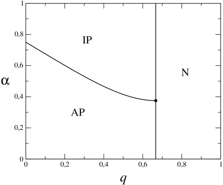
Figure 2: Phase diagram from the pair approximation in the plane $\alpha=\lambda^{-1}$ versus $q=1-p$, for a lattice of coordination $k=4$. The phases are: active percolating (AP), inactive percolating (IP), and nonpercolating (N).

Using again the pair approximation and the previous notation together with the notations $z=P_{I}$, $g=P_{IE}$, $h=P_{IU}$, we may write

$$\frac{dz}{dt}=-rz+cg,$$ (24)

$$\frac{dg}{dt}=-rg+r(z-g-h)-\frac{c}{k}g-c\mu\frac{g^{2}}{y}+c\mu\frac{g}{y}(y-g-w),$$ (25)

$$\frac{dh}{dt}=-rh+c\mu\frac{gw}{y},$$ (26)

where we have taken into account that $P_{II}=P_{I}-P_{IE}-P_{IU}=z-g-h$ and $P_{EE}=P_{E}-P_{EI}-P_{EU}=y-g-w$.

Equations (24)-(26) are to be solved using as initial conditions the stationary state of the first model. Since $P_{E}+P_{I}=y+z$ is invariant, it follows that $y+z=y_{0}$ where $y_{0}$ is the value of $P_{E}$ at the stationary state of the first model, given by equation (14). Analogously, $P_{EU}+P_{IU}=w+h$ is invariant implying $w+h=w_{0}$ where $w_{0}$ is the value of $P_{EU}$ at the stationary state of the first model, given by equation (17). At stationary state, equations (24)-(26) have a trivial solution $z=0$, characterizing the absorbing state, and a nontrivial solution for which $z\neq 0$, characterizing the active state. Solving for $z$, it is possible to obtain an expression for the nontrivial solution $z$. By taking the limit $z\to 0$ of the nontrivial solution we get the critical line, which is given by

$$\alpha=\frac{r}{c}=\frac{k-1}{k}\left(1-\frac{q(1-s)}{p(1-s^{k})}\right),$$ (27)

where $s$ is the root of the polynomial equation given by equation (18). The critical line $\alpha$ versus $q$, shown in figure 2, separates the active percolating phase from the inactive percolation phase. Notice that, when $p\to p_{c}=1/(k-1)$ we get $\alpha=2(k-1)/k^{2}=\alpha_{0}$, so that the critical line meet the vertical line $p=p_{c}$ at $\alpha=\alpha_{0}$, as shown in figure 2. It straightforward to show that the critical exponent related to the order parameter is the same as that of the pure system.

3 Scaling relations and numerical simulations

Around the critical point, the quantities that characterize the critical behavior are assumed to obey scaling relations. In the present case of the diluted contact model, for which the quenched disorder is relevant, the usual scaling relation in terms of power laws in time is replaced by power laws in the logarithm of time, called activated scaling [11, 12]. At the critical point, the space correlation length $\xi$ behaves as [12]

$$\xi\sim(\ln t/t_{0})^{1/\psi},$$ (28)

where $\psi$ is the tunneling critical exponent [15] and $t_{0}$ is a constant. Other quantities behave similarly at the critical point, such as $N_{I}$, the number of infected individuals,

$$N_{I}\sim(\ln t/t_{0})^{\theta},$$ (29)

and $P$, the survival probability at time $t$,

$$P\sim(\ln t/t_{0})^{-\delta}.$$ (30)

From the scaling relations (28), (29), and (30) we find that

$$N_{I}\sim P^{-\theta/\delta},$$ (31)

$$N_{I}\sim\xi^{\,\theta\,\psi},$$ (32)

$$P\sim\xi^{-\delta\psi},$$ (33)

valid at the critical point. These are useful relations because they do not depend on $t_{0}$.

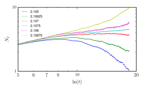
Figure 3: Log-log plot of the number of infected sites $N_{I}$ versus $t$ obtained from numerical simulations at $p=0.8$ for the values of $\lambda$ indicated.

At the stationary state ($t\to\infty$), the quantities that describe the critical behavior follow the usual power laws, but with exponents distinct from those of the pure system. The order parameter $\rho$, defined as the fraction of infected sites in the percolating cluster, behaves as

$$\rho\sim(\lambda-\lambda_{c})^{\beta}.$$ (34)

Initially, we have simulated the first model to generate a percolating cluster. The simulation, with periodic boundary conditions, was performed as follows. At each time step, we choose at random a bond from a list of active bonds. An active bond is a pair of SE nearest neighbor sites. The site S of the chosen bond becomes E with probability $p$ and becomes U with the complementary probability $q=1-p$. The chosen bond is removed from the list and the list us updated. The time is then incremented by an amount $1/N_{a}$, where $N_{a}$ is the number of active bonds in the list. Notice that, if a site S has $n_{E}$ nearest neighbor sites in states E, then it will appear $n_{E}$ times in the list. Starting with just one E site in a lattice full of S sites, this algorithm will generate a cluster of E sites. This process stops when there is no SE bonds in the lattice. When this happens the cluster of E sites is a site percolating cluster with U sites standing in the border of the cluster, separating the E sites from the S sites.

Having generated a percolating cluster of E sites, we simulate the contact model on top of the cluster using the following algorithm. At each time step, a site is chosen at random among a list of I sites. With probability $p_{a}=\lambda/(\lambda+1)$ it becomes an E site and with the complementary probability $1-p_{a}$ a nearest neighbor site is chosen at random. If the chosen neighboring site is in state E, it becomes I, otherwise, nothing happens. The time is then incremented by an amount $1/N_{I}$, where $N_{I}$ is the number of I sites. The initial condition is formed by the cluster of E sites with one E site turned into an I site. This I site is taken as the origin.

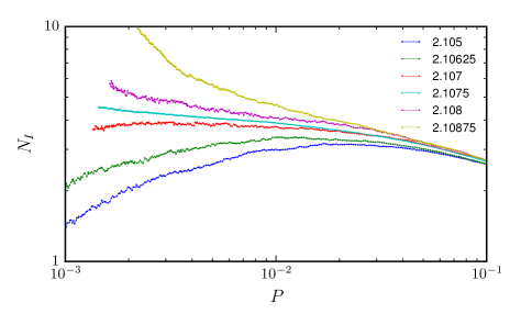
Figure 4: Log-log plot of the number of infected sites $N_{I}$ as a function of the survival probability $P$ obtained from numerical simulations at $p=0.8$ for the values of $\lambda$ indicated.

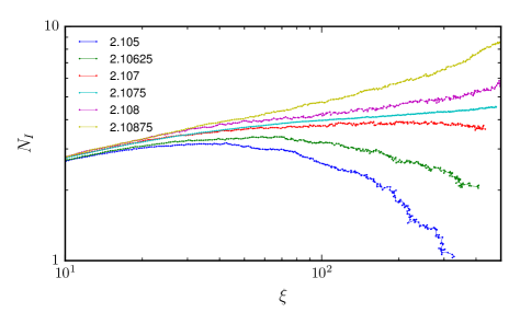
Figure 5: Log-log plot of the number of infected sites $N_{I}$ as a function of the spatial correlation length $\xi$ obtained from numerical simulations at $p=0.8$ for the values of $\lambda$ indicated.

We have performed simulations on a square lattice with $N=L^{2}$ sites with $L$ up to $L=8192$. For several values $p$ and $\lambda$, we have measured, as a function of time, the number of infected sites $N_{I}$, the survival probability $P$ and the correlation length $\xi$ defined by

$$\xi^{2}=\frac{1}{N_{I}}\sum_{i}\langle r_{i}^{2}\rangle,$$ (35)

where the summation is over the sites occupied by an infected and $r_{i}$ is the distance from the site $i$ to the origin. Each quantity was measured by averaging over $10^{5}$ to $10^{6}$ disorder configurations, where each disorder configuration is obtained by the simulation of the first model starting with a distinct seed of random number. We have also performed simulation with smaller values of $L$. However, results coming from lattice with $L=4096$ agree, within statistical errors and up to the maximum time we have used, with those coming from $L=8192$. The statistical errors were determined by the calculation of the standard statistical deviation. The results for the three quantities $N_{I}$, $P$ and $\xi$, determined for several values of $\lambda$, are shown in figures 3, 4, and 5. The error bars in these figures are not shown, but they are less than 8%. At the critical point, $\lambda=2.1075$, they are even less reaching 1%.

Figure 3 shows the plot of the number of infected $N_{I}$ as a function of time $t$ for $p=0.8$. Fitting the expression (29) to the data points of figure 3 we estimate the critical parameter as being $\lambda=2.1075(1)$, the critical exponent as $\theta=0.13(2)$, and $\ln t_{0}=6.0(5)$. To find the exponents $\psi$ and $\delta$ and a better estimate of $\theta$ we use a procedure similar to the one used in [11] in which we first determine the quantities $\theta/\delta$, $\theta\,\psi$ and $\delta\psi$, by fitting the expressions (31), (32) and (33) to the data points. After that, we use expressions (28), (29) and (30) to find the exponents $\theta$, $\delta$ and $\psi$ by a constrained fitting, to be explained below.

From the plots of $N_{I}$ versus $P$, shown in figure 4, $N_{I}$ versus $\xi$, shown in figure 5, and $P$ versus $\xi$, we may get, respectively, $\theta/\delta$, $\theta\,\psi$ and $\delta\psi$. Since the scaling relations (31) (32) and (33) do not involve time, the estimates of these quantities are independent of the $t_{0}$, resulting in more precise values, which are found to be

$$\theta/\delta=0.075(5),$$ (36)

$$\theta\,\psi=0.078(4)$$ (37)

$$\delta\psi=1.034(23).$$ (38)

The consistency of these values can be checked by dividing equations (37) and (38). The result is $\theta\,\psi/\delta\psi=0.0758(57)$, which is in fair agreement with (36). The value of $\theta/\delta$ can be used to get the ratio $\beta/\nu_{\perp}$ between the order parameter critical exponents $\beta$ and the critical exponents $\nu_{\perp}$ related to the spatial correlation length. Using the relation $\theta/\delta=d\nu_{\perp}/\beta-2$ we find

$$\beta/\nu_{\perp}=0.964(2).$$ (39)

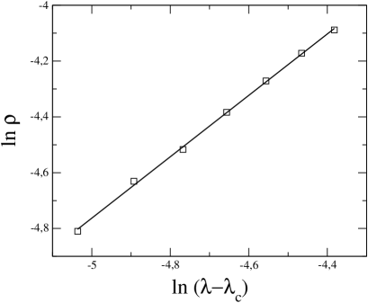
Figure 6: Fraction of infected sites $\rho$ in the percolating cluster as a function of $\lambda$. The slope of the strait line fitted to the data points gives $\beta=1.11(6)$.

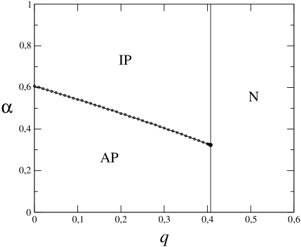
Figure 7: Phase diagram from numerical simulations on a square lattice in the plane $\alpha=\lambda^{-1}$ versus $q=1-p$. The phases are: active percolating (AP), inactive percolating (IP), and nonpercolating (N).

The exponents $\theta$, $\delta$ and $\psi$ are found by a procedure as follows. For each value of $t_{0}$ in the interval $5.5\leq t_{0}\leq 6.5$, we determine the exponents $\theta$, $\delta$ and $\psi$ by fitting the expressions (28), (29) and (30) to the data points. After that we choose the actual values of these exponents as the ones such that the quantities $\theta/\delta$, $\theta\,\psi$ and $\delta\psi$ are as close as possible to the values given by (36), (37), (38). This procedure leads to the following values for the exponents:

$$\theta=0.145(8),$$ (40)

$$\delta=1.88(11),$$ (41)

$$\psi=0.55(3).$$ (42)

Table 1: Critical exponents obtained by numerical simulations on a square lattice at $p=0.8$ and $\lambda_{c}=2.1075$ (second column). The third and fourth columns show results for the quenched diluted contact process [10, 11] in $d=2$ whereas the last two columns show results for the random transverse-field Ising model [16, 20] also in $d=2$.

ref.	this work	[10]	[11]	[16]	[20]
$\theta$	$0.145(8)$		$0.15(3)$
$\psi$	$0.55(3)$	$0.48(7)\,$	$0.51(6)$	$0.42(6)$	$0.48(2)$
$\delta$	$1.88(11)$		$1.9(2)$
$\phi$	$1.87(10)$			$2.5(4)$
$\beta/\nu_{\perp}$	$0.964(2)$	$0.95(2)\,$	$0.96(2)$	$1.0(1)$	$0.982(15)$
$\beta$	$1.11(6)$		$1.15(9)$
$\nu_{\perp}$	$1.15(6)$		$1.20(15)$	$1.07(15)$	$1.24(2)$
$d_{F}$	$1.036(2)$			$1.0(1)$	$1.018(15)$

We have also performed simulations to get the stationary properties by using systems of linear size $L=2048$. The interest quantities were obtained by the use of $10^{8}$ Monte Carlo steps after discarding $10^{7}$ Monte Carlo steps. In this case, we use as the initial state a configuration in which a fraction of sites is in the infected state. Again we determined the number of infected sites $N_{I}$ at the stationary state from which we obtained the density $\rho=N_{I}/N_{C}$ where $N_{C}$ is the number of sites of the cluster, that is, the number of I sites plus the number of E sites. Assuming the critical behavior (34), we get the value $\beta=1.11(6)$ by plotting $\rho$ as a function of $\lambda-\lambda_{c}$, as shown in figure 6 for the case of $p=0.8$. This result for $\beta$ together with the numerical value for the ratio $\beta/\nu_{\perp}$, obtained above, gives us $\nu_{\perp}=1.15(6)$.

We have also performed similar simulations for other value of $p$ and obtained the critical line, shown in figure 7. In particular, at the percolation critical point $p=p_{c}=0.59274$, we get $\lambda=3.10(1)$.

The critical exponents obtained here are shown in table 1 together with results coming from other papers on the quenched diluted contact process [11, 10] and on the random transverse-field Ising model [16, 20]. To make contact with exponents used to describe the critical behavior of the random transverse-field Ising model, we have determined from our results the fractal dimension critical exponent $d_{F}=d-\beta/\nu_{\perp}$ and the exponent $\phi$, related to the fractal dimension and the tunneling exponent by $d_{F}=\phi\psi$ [16]. We see that our results agree, within the statistical errors, to all other results cited in table 1. The results are $d_{F}=1.036(2)$ and $\phi=1.87(10)$.

4 Conclusion

We have studied the critical properties of the quenched diluted contact process through a mean-field theory and Monte Carlo simulations by using a two stage procedure. The first was the generation of the percolating cluster, obtained by the use of a stochastic lattice model whose stationary states are the clusters of percolation model. The second stage was the simulation of the contact process on the top of the percolating cluster. It should be remarked that, only the percolating clusters is necessary if we wish to study the static stationary properties because finite clusters cannot support an active state. For a finite cluster, the absorbing state will be reached if we wait enough time. As to the dynamic properties, our results show that they can also be obtained from the percolating cluster, or at least their critical properties, as can be inferred by comparing our critical exponents with other works. The present method allowed to obtain more precise critical exponents, with errors that are at most equal to 6%, confirming the prediction that the quenched diluted contact process belongs to the universality class of the random transverse-field Ising model.

The mapping of the two epidemic models into the quenched diluted contact process allows to speculate about the existence of epidemic models that are in the universality class of transverse-field Ising model. In fact, this is the case of the model illustrated in figure 8, which may be thought as a merger of the two models in figure 1. The epidemic model of figure 8 is defined on a lattice in which each site can be in one of four states: S, U, E, and I, and is composed by three catalytic reactions: S $\to$ U, S $\to$ E, E $\to$ I, and by a spontaneous reaction I $\to$ E. At the stationary states, the I and E sites form a connected cluster of sites consisting of a site percolation cluster. The E and I sites evolves then as the contact process on the top of a percolating cluster. Therefore, the model defined by rules of figure 8 is also mapped into the quenched diluted contact process and its critical properties puts the model in the universality class of the transverse-field Ising model.

Figure 8: The processes S $\to$ U and S $\to$ E are catalytic with E or I playing the role of catalysts. The process E $\to$ I is autocatalytic and the reaction I $\to$ E is spontaneous.

References

References

- [1] A. B. Harris, J. Phys. C 7, 1671 (1974).
- [2] T. E. Harris, Ann. Prob. 2, 969 (1974).
- [3] J. Marro and R. Dickman, Noequilibrium Phase Transitions in Lattice Models, (Cambridge University Press, Cambridge, 1999).
- [4] M. Henkel, H. Hinrichesen and S. Lübeck, Non-Equilibrium Phase Transitions, Vol. I: Absorbing Phase Transitions (Springer, Dordrecht, 2008).
- [5] T. Tomé and M. J. de Oliveira, Stochastic Dynamics and Irreversibility, Springer, 2015.
- [6] A. G. Moreira and R. Dickman, Phys. Rev. E 54, R3090 (1996).
- [7] R. Dickman and A. G. Moreira, Phys. Rev. E 57, 1263 (1998).
- [8] T. Vojta and M. Dickison, Phys. Rev. E 72, 036126 (2005).
- [9] S. R. Dahmen, L. Sittler and H. Hinrichsen, J. Stat. Mech. P01011 (2007).
- [10] M. M. de Oliveira and S. C. Ferreira, J. Stat. Mech. P11001 (2008).
- [11] T. Vojta, A. Farquhar and J. Mast, Phys. Rev. E 79, 011111 (2009).
- [12] J. Hooyberghs, F. Iglói, and C. Vanderzande, Phys. Rev. Lett. 90, 100601 (2003).
- [13] J. Hooyberghs, F. Iglói, and C. Vanderzande, Phys. Rev. E 69, 066140 (2004).
- [14] D. S. Fisher, Phys. Rev. Lett. 69, 534 (1992).
- [15] D. S. Fisher, Physica A 263, 222 (1999).
- [16] O. Motrunich, S. C. Mau, D. Huse, and D. S. Fisher, Phys. Rev. B 61, 1160 (2000).
- [17] Y.-C. Lin, N. Kawashima, F. Iglói, and H. Rieger, Prog. Theor. Phys. Supplement 138 479 (2000).
- [18] D. Karevski, Y-C. Lin, H. Rieger, N. Kawashima and F. Iglói, Eur. Phys. J. B 20, 267 (2001).
- [19] J. A. Hoyos, Phys. Rev. E 78, 032101 (2008).
- [20] I. A. Kovács and F. Iglói, Phys. Rev. B 82, 054437 (2010).
- [21] R. Miyazaki and H. Nishimori, Phys. Rev. E 87, 032154 (2013).
- [22] T. Tomé and R. M. Ziff, Phys. Rev. E 82, 051921 (2010).
- [23] T. Tomé and M. J. de Oliveira, J. Phys. A 44, 095005 (2011).
- [24] A. H. O. Wada, T. Tomé and M. J. de Oliveira, J. Stat. Mech. P04014 (2015).
- [25] H. Hinrichsen, Braz. J. Phys. 30, 69 (2000).
- [26] K. A. Takeuchi, M. Kuroda, H. Chaté, and M. Sato, Phys. Rev. Lett. 99, 234503 (2007).