Asymmetric noise-induced large fluctuations in coupled systems

Abstract

Networks of interacting, communicating subsystems are common in many fields, from ecology, biology, epidemiology to engineering and robotics. In the presence of noise and uncertainty, interactions between the individual components can lead to unexpected complex system-wide behaviors. In this paper, we consider a generic model of two weakly coupled dynamical systems, and show how noise in one part of the system is transmitted through the coupling interface. Working synergistically with the coupling, the noise on one system drives a large fluctuation in the other, even when there is no noise in the second system. Moreover, the large fluctuation happens while the first system exhibits only small random oscillations. Uncertainty effects are quantified by showing how characteristic time scales of noise induced switching scale as a function of the coupling between the two coupled parts of the experiment. In addition, our results show that the probability of switching in the noise-free system scales inversely as the square of reduced noise intensity amplitude, rendering the virtual probability of switching to be an extremely rare event. Our results showing the interplay between transmitted noise and coupling are also confirmed through simulations, which agree quite well with analytic theory.

I Introduction

Understanding the interaction between noise and system dynamics is key to understanding unexpected system behaviors Gardiner (2004); Van Kampen (2007), and hence to robust and efficient operation of autonomous systems deployed in noisy, uncertain environments. It is often assumed that dynamics with small noise input can be modeled as small perturbations of the deterministic system dynamics; however, there are many known cases where small noise inputs can drive large-scale transitions in system behavior. Examples include noise-induced switching between attractors in continuous systems Freidlin and Wentzell (1984); Doering and Gadoua (1992); Castellano et al. (1996); Lapidus et al. (1999); Kim et al. (2005); Siddiqi et al. (2005); Chan and Stambaugh (2007); Dykman and Schwartz (2012); D’Huys et al. (2014); Emenheiser et al. (2016); Huang et al. (2016), and noise-induced switching and extinction in finite-size systems Allen et al. (2005); Barzel and Biham (2008); Kamenev et al. (2008); Kamenev and Meerson (2008); Dykman et al. (2008); Wells et al. (2015); Chen et al. (2016); Hindes and Schwartz (2016).

In both switching and extinction, a significant change in the state of the system occurs as the result of a noise-induced large fluctuation. For systems with small noise, such a large fluctuation is a rare event, and occurs on average when the noise signal lies along a so-called “optimal path” Schwartz et al. (2011). For systems operating in most common environments, noise is assumed to be homogeneous, and it is relatively straight-forward to compute the optimal paths which lead to large fluctuations Dykman (1990).

In contrast to homogeneous noise, finite systems, whether continuous or discrete, are often subject to asymmetric noise Le Masne et al. (2009); Ankerhold and Pechukas (1999). One excellent example of multiple independent noise sources occurs in coupled finite communicating systems operating in noisy environments Lindley et al. (2013), where the effects of noise on the collective motions of swarms of self-propelled autonomous agents results in drastic pattern changes. Such systems are of tremendous practical importance; coordinated groups of agents have been deployed for a wide range of applications, including exploration and mapping of unknown environments Earon et al. (2001); Benerjee and Deepthi (2015); Bhattacharya et al. (2012); Lynch et al. (2008); Wu and Zhang (2011), search and rescue Takano et al. (2014); Al Tair et al. (2015), and construction Augugliaro et al. (2014). Extensions to the basic swarming dynamics by using teams of heterogeneous agents capable of cooperatively executing more complex tasks are presented in Ramp et al. (2009); Dorigo et al. (2013). In addition, network structure and uncertainties in delay communication have been shown to give rise to dynamic patterns in collective swarm motion Szwaykowska et al. (2016a); Hindes et al. (2016).

Usually, sophisticated models are used to predict behavioral patterns for large groups of interacting individual agents Ben-Jacob et al. (1997); Calovi et al. (2014); Carlen et al. (2013); Hsieh et al. (2008). However, testing these behaviors in real-world environments often presents significant logistical challenges. In many cases, it is more practical to rely on mixed-reality experiments (similar to ideas in Gintautas and Hübler (2007)), where real agents are deployed alongside simulated ones, in order to better understand how real-world noise affects the collective dynamics, as well as validate the theory against a critical number of agents Szwaykowska et al. (2016b). This creates a situation where we have two coupled systems with asymmetric noise characteristics: the set of real agents, operating in a high-noise real-world environment, and the simulated agents, operating in a (at least partly) idealized simulated world. Our current paper is inspired by this situation; we consider a generic pair of coupled dynamical systems, and study the effects of interaction on switching in the low-noise system.

As shown e.g. in Kozlov et al. (2016), even weak coupling between system dynamics can significantly affect the behavior of the coupled systems. We show that even weak interaction between a low noise, or noise-free, simulated system and a noisy “real” system can cause catastrophic transitions between states. That is to say, even if only part of the system operates in noisy real-world conditions, we can observe large changes in the dynamics of the idealized, low-noise virtual part, since noise is transmitted from the real to virtual world via coupling. Since one of our main results shows how the probability exponent is enhanced by the ratio of two noise sources, we refer to the state transitions induced in the noise-free virtual system by coupling with the noisy real-world system as extreme rare events.

The rest of the paper is laid out as follows. In Section II we define the general asymmetric noise problem for coupled systems (which include MR systems). Gaussian noise is considered here, but the theory can be made more general to include non-Gaussian perturbations Dykman (2010) and correlations Feynman and Hibbs (1965a); Dykman (1990). Noise induced large fluctuations are posed in a variational setting for the coupled problem. Linear response to the noise is derived in general. In Section III, we consider a model problem of coupled bi-stable attractors subjected to asymmetric noise. For the specific problem we compare our theory to Monte Carlo simulations, and derive scalings as a function of the heterogeneity of the noise. We derive a general scaling relation between the noise ratio and the coupling strength that governs the mean probability to switch. To quantify the extreme rare event of the low-noise system switching, we derive the exponent of the probability distribution, and show that this exponent varies as the inverse noise ratio squared. Comparisons between our general theory and numerical experiments of such large fluctuation events show excellent agreement. A discussion of the results and conclusions are given in Section IV.

II Problem Setup in General

The problem formulation described here is motivated by the mixed-reality system shown in Fig. 1. In this setup, the physical agents operate in an uncertain, noise-ridden environment, which imposes a larger noise source on all of the agents. In contrast, the virtual agents are isolated from any real environmental perturbations, and experience only the noise modeled in the simulation. We let the time dependent vectors ${\bm{x},\bm{y}}$ denote the state-space configurations of agents operating in virtual and real environments, respectively.

We wish to examine the situation where there is a significant asymmetry in the noise characteristics of the two coupled systems; in particular, where the noise intensity in the low-noise (“virtual”) system goes to zero.

Figure 1: Experimental setup with virtual swarm of agents. The real robots operate in a lab testbed. The positions of the real and simulated agents are passed to the virtual swarm simulator, which models the response of the virtual swarm agents to the current swarm configuration; and to the controller, which computes the real robot response and passes target velocities to the real swarm agents. The agents use internal proportional $-$ integral $-$ derivative (PID) controllers to achieve the target velocities.

II.1 The stochastic equations of motion

To analyze how noise impacts the dynamics from one environment to another, we consider a general coupled stochastic differential equation of the form

$$\dot{\bm{x}}(t) =\bm{f}(\bm{x}(t))+{\bf h}_{1}(\bm{x}(t),\bm{y}(t),K)+\epsilon\bm{G}_{1}({\bm{x}}(t))\bm{\xi_{x}}(t),$$ (1a)

$$\dot{\bm{y}}(t) =\bm{f}(\bm{y}(t))+{\bf h}_{2}(\bm{x}(t),\bm{y}(t),K)+\bm{G}_{2}(\bm{y}(t))\bm{\xi_{y}}(t),$$ (1b)

where $\bm{x}\in\mathbb{R}^{n_{x}}$ and $\bm{y}\in\mathbb{R}^{n_{y}}$ represent the state-space configurations of the low- and high-noise systems, respectively, and the matrices ${\bm{G}}_{i}$, $i=1,2$ are given by $\bm{G}_{i}(\bm{x}(t))=\text{diag}\{g_{i1}(\bm{x}(t)),g_{i2}(\bm{x}(t)),...g_{in_{i}}(\bm{x}(t))\}$, where the $g_{ij}$’s are general nonlinear functions. Coupling strength is denoted by parameter $K$, and we choose ${\bf h}_{1}$, ${\bf h}_{2}$ so that ${\bf h}_{1}(\bm{x}(t),\bm{y}(t),0)={\bf h}_{2}(\bm{x}(t),\bm{y}(t),0)=0$; i.e., the systems $\bm{x},\bm{y}$ are uncoupled when $K=0$.

We assume that the noise inputs $\bm{\xi}_{x}\in\mathbb{R}^{n_{x}}$ and $\bm{\xi}_{y}\in\mathbb{R}^{n_{y}}$ are independent Gaussian-distributed stochastic processes with independent components, and intensity $D$. They are both characterized by a probability density functional $\mathcal{P}_{\bm{\xi}}=e^{-\mathcal{R}_{\xi}/D}$, where $\mathcal{R}_{\xi}$ is defined as

$${\cal R}_{{\bm{\xi}}}[{\bm{\xi}}(t)]=\frac{1}{4}\int dt\,dt^{\prime}\,{\bm{\xi}}(t){\bm{\xi}}(t^{\prime}).$$ (2)

In order to capture the asymmetric noise levels between the two systems, we introduce a parameter, $\epsilon\ll 1$, that controls the noise intensity of the state variable ${\bm{x}}$. The case $\epsilon=0$ corresponds to noise-free operation. However, even with $\epsilon=0$, noise-induced transitions can still occur as a result of noise transference through the coupling with the high-noise system.

II.2 Deterministic dynamics

In the absence of any noise, Eqs. 1 are ordinary differential equations, and we suppose that there exist steady states which depend on the coupling strength, $K$. We therefore assume that there exists an attracting equilibrium $({\bm{x}}_{a}(K),{\bm{y}}_{a}(K))$ and at least one saddle equilibrium point, $({\bm{x}}_{s}(K),{\bm{y}}_{s}(K))$.

The stationary states satisfy.

$$\bm{f}(\bm{x}_{a})+{\bf h}_{1}(\bm{x}_{a},\bm{y}_{a},K) =\bm{f}(\bm{x}_{s})+{\bf h}_{1}(\bm{x}_{s},\bm{y}_{s},K)=0$$ (3a)

$$\bm{f}(\bm{y}_{a})+{\bf h}_{2}(\bm{x}_{a},\bm{y}_{a},K) =\bm{f}(\bm{y}_{s})+{\bf h}_{2}(\bm{x}_{s},\bm{y}_{s},K)=0.$$ (3b)

The stability of the equilibrium states is given by the linear variational equations of motion about that state:

$$\dot{\bf X}(t)={\bf{\cal M}}({\bar{\bm{x}}},{\bar{\bm{y}}},K){\bf X}(t),$$ (4)

where ${\bar{\bm{x}}},{\bar{\bm{y}}}$ denote either $\bm{x}_{a},\bm{y}_{a}$ or $\bm{x}_{s},\bm{y}_{s}$, and

$${\bf{\cal M}}({\bar{\bm{x}}},{\bar{\bm{y}}},K)=\begin{bmatrix}\frac{\partial{\bf f}({\bar{\bm{x}}})}{\partial x}+\frac{\partial{\bf h}_{1}({\bar{\bm{x}}},{\bar{\bm{y}}},K)}{\partial x}&\frac{\partial{\bf h}_{1}({\bar{\bm{x}}},{\bar{\bm{y}}},K)}{\partial y}\\ \frac{\partial{\bf h}_{2}({\bar{\bm{x}}},{\bar{\bm{y}}},K)}{\partial x}&\frac{\partial{\bf f}({\bar{\bm{y}}})}{\partial y}+\frac{\partial{\bf h}_{2}({\bar{\bm{x}}},{\bar{\bm{y}}},K)}{\partial y}\end{bmatrix}.$$

The matrix ${\bf{\cal M}}({\bar{\bm{x}}},{\bar{\bm{y}}},K)$ evaluated at the saddle point is assumed to have only one positive real eigenvalue (associated with an unstable direction in the space of dynamical variables), while the rest of the eigenvalue spectrum lies in the left hand side of the complex plane. In particular, we assume that for all values of interest $K$, the saddle point lies on the basin boundary of the attractor. The generic switching scenario occurs for arbitrarily small noise when the dynamics in one basin approaches the stable manifold of the saddle point, which guides the dynamics to the saddle. Once in the neighborhood of the saddle point, noise may cause the switch from one basin to another along the direction of the unstable manifold associated with the unstable eigenvalue.

When noise is added to the system, we wish to compute the probability of escaping from the basin of attraction of attractor $(\bm{x}_{a},\bm{y}_{a})$. The asymmetry of the noise between the virtual and real agents is controlled by $\epsilon$, which scales the noise intensity of ${\bm{x}}$. Computing the probability of escape in the small noise limit implies that we compute the most likely paths which cross the basin boundary of the attractor at the saddle point $(\bm{x}_{s},\bm{y}_{s})$. In describing the effect of how noise bleeds into the virtual world from the real world, we want to measure noise-induced changes that are large in the dynamics of the state of ${\bm{x}}$ while ${\bm{y}}$ remains approximately stationary; i.e., ${\bm{y}}$ does not change as much as ${\bm{x}}$. Thus, in the presence of noise, we are interested in describing how the most likely path develops when ${\bm{x}}_{a}(K)$ changes its position much more than ${\bm{y}}_{a}(K)$. In order to focus on this case, we assume that, when noise and coupling are both 0, ${\bm{x}}_{a}(0)$ lies in a different part of phase space than ${\bm{y}}_{a}(0)$. Correspondingly, we also assume that $||{\bm{x}}_{a}(K)-{\bm{x}}_{s}(K)||\gg||{\bm{y}}_{a}(K)-{\bm{y}}_{s}(K)||$, while $||{\bm{y}}_{a}(K)-{\bm{y}}_{s}(K)||\ll 1$ given that the equilibria depend smoothly on the coupling strength $K$. We note, however, that these assumptions do not affect the general theory, and our methods could be equally well applied if these assumptions were dropped.

II.3 The Variational Formulation of Noise Induced Escape

For a given coupling $K$, we wish to determine the path with the maximum probability of noise induced switching from the initial attracting state $({\bm{x}}_{a}(K),{\bm{y}}_{a}(K))$ to another $({\bm{x}}_{b}(K),{\bm{y}}_{b}(K))$, where the initial and final states are equilibria of the noise-free versions of Eqs. 1. Each attractor possesses its own basin of attraction, and therefore on average, small noise is expected to induce small fluctuations about the stable equilibria. However, sometimes the noise will organize itself in such a way that a large fluctuation occurs, allowing escape over the effective energy barrier away from the stable equilibrium. If the fluctuation is sufficiently large to bring the system state close to the saddle point, there is a possibility of switching. Near the saddle point, depending on the sign of the projection of the local trajectory onto the unstable manifold of the positive eigenvalue, the system will approach one or the other attractor. Switching occurs once the trajectory enters a different basin of attraction from the one where it started.

We assume the noise intensity $D$ is much smaller than the effective barrier height, and that the scaling on the noise input $\epsilon$ satisfies $0\leq\epsilon<1$. Note that the noise terms $({\bm{\xi}}_{\mathbf{x}},{\bm{\xi}}_{\mathbf{y}})$ are formally the time derivative of a Brownian motion, sometimes referred to as white noise Fleming and Rishel (1975).

For $D$ sufficiently small, we make the ansatz that the probability distribution of observing such a large fluctuation scales exponentially as the inverse of $D$ Freidlin and Wentzell (1984); Dykman (1990),

$$\mathcal{P}_{x}=e^{-R/D},$$ (5)

where

$$R(K)=\min_{(\bm{x},\bm{y},\bm{\xi}_{x},\bm{\xi}_{y},\bm{\lambda_{1}},\bm{\lambda_{2}})}\mathcal{R}(\bm{x},\bm{y},\bm{\xi}_{x},\bm{\xi}_{y},\bm{\lambda_{1}},\bm{\lambda_{2}};K),$$ (6)

and

$$\mathcal{R}(\bm{x},\bm{y},{\bm{\xi}}_{x},{\bm{\xi}}_{y},\bm{\lambda_{1}},\bm{\lambda_{2}};K)=R_{{\bm{\xi}}_{x}}[{\bm{\xi}}_{x}(t)]+R_{{\bm{\xi}}_{y}}[{\bm{\xi}}_{y}(t)]\\ +\int_{-\infty}^{\infty}dt\bm{\lambda_{1}}(t)\cdot[\dot{\bm{x}}(t)-\bm{f}(\bm{x}(t))-{\bf h}_{1}(\bm{x}(t),\bm{y}(t),K)-\epsilon\bm{G}_{1}({\bm{x}}(t)){\bm{\xi}}_{x}(t)]\\ +\int_{-\infty}^{\infty}dt\bm{\lambda_{2}}(t)\cdot[\dot{\bm{y}}(t)-\bm{f}(\bm{y}(t))-{\bf h}_{2}(\bm{x}(t),\bm{y}(t),K)-{\bm{G}}_{2}(\bm{y}(t)){\bm{\xi}}_{y}(t)].$$ (7)

We will see later that the Lagrange multipliers, $\bm{\lambda}_{1},\bm{\lambda}_{2}$, also correspond to the conjugate momenta of the equivalent Hamilton-Jacobi formulation of this problem . Similar to classical mechanics, the exponent $R$ of Eq. 5 is called the action, and corresponds to the minimizer of the action in the Hamilton-Jacobi formulation which occurs along the optimal path Feynman and Hibbs (1965a). This path will minimize the integral of Eq. 7, and is found by setting the variations along the path $\delta\mathcal{R}$ to zero. The transition rate exponent is proportional to the action, $R$.

When computing the action, the boundary conditions are important, especially since in general they depend on the parameters of the problem. Therefore, we suppose that dynamics starts near the attractor $(\bm{x}_{a},\bm{y}_{a})$. Small fluctuations will on average remain in the basin of the attractor until at some point in time, the dynamics hits the saddle point, $(\bm{x}_{s},\bm{y}_{s})$. Thus, we have the boundary conditions given by:

$$\lim_{t\rightarrow-\infty}({\bm{x}}(t),{\bm{y}}(t)) =({\bm{x}}_{a}(K),{\bm{y}}_{a}(K))$$ (8)

$$\lim_{t\rightarrow\infty}({\bm{x}}(t),{\bm{y}}(t)) =({\bm{x}}_{s}(K),{\bm{y}}_{s}(K)).$$ (9)

To examine the structure of the Hamiltonian governing the large fluctuations, we take the variational derivative of $\mathcal{R}(\bm{x},\bm{y},{\bm{\xi}}_{x},{\bm{\xi}}_{y},\bm{\lambda_{1}},\bm{\lambda_{2}};K)$ with respect to the noise sources, $\bm{\xi}_{i}$ (where $i=\bm{x},\bm{y}$). Setting the derivative equal to 0 gives

$$\bm{\xi_{x}} =2\epsilon\bm{G}_{1}({\bm{x}})\bm{\lambda}_{1}$$ (10)

$$\bm{\xi_{y}} =2\bm{G}_{2}({\bm{y})}\bm{\lambda}_{2}.$$ (11)

The full set of equations of motion is then derived by taking the variational derivatives with respect to the state variables and their corresponding momenta:

$$\dot{\bm{x}} =\bm{f}(\bm{x})+{\bf h}_{1}(\bm{x},\bm{y},K)+2\epsilon^{2}\bm{G_{1}}^{2}(\bm{x})\bm{\lambda}_{1}$$ (12)

$$\dot{\bm{\lambda}_{1}} =-\epsilon^{2}\bm{G_{1}(x)}{\frac{\partial\bm{G_{1}}{(\bm{x})}}{\partial\bm{x}}}\bm{\lambda}_{1}\bm{\lambda}_{1}-\frac{\partial(\bm{f}(\bm{x})+{\bf h}_{1}(\bm{x},\bm{y},K))}{\partial\bm{x}}\bm{\lambda}_{1}$$

$$-\frac{\partial({\bf h}_{2}(\bm{x},\bm{y},K))}{\partial\bm{x}}\bm{\lambda}_{2}$$

$$\dot{\bm{y}} =\bm{f}(\bm{y})+{\bf h}_{2}(\bm{x},\bm{y},K)+2\bm{G_{2}}^{2}({\bm{y}})\bm{\lambda}_{2}$$

$$\dot{\bm{\lambda}_{2}} =-\bm{G_{2}(y)}{\frac{\partial\bm{G_{2}}{(\bm{y})}}{\partial\bm{y}}}\bm{\lambda}_{2}\bm{\lambda}_{2}-\frac{\partial(\bm{f(y)}+{\bf h}_{2}(\bm{x},\bm{y},K))}{\partial\bm{y}}\bm{\lambda}_{2}$$

$$-\frac{\partial({\bf h}_{1}(\bm{x},\bm{y},K))}{\partial\bm{y}}\bm{\lambda}_{1}.$$

The full Hamiltonian is derived by substituting the ansatz in Eq. 5 into the appropriate Fokker-Planck equation and dropping terms of order higher than $1/D$, which results in a Hamilton-Jacobi equation with Hamiltonian:

$$H =[\epsilon^{2}\bm{G_{1}}^{2}(\bm{x})\bm{\lambda}_{1}]\cdot\bm{\lambda}_{1}+[\bm{G_{2}}^{2}(\bm{y})\bm{\lambda}_{2}]\cdot\bm{\lambda}_{2}$$ (13)

$$+\bm{\lambda}_{1}\cdot[\bm{f}(\bm{x})+{\bf h}_{1}(\bm{x},\bm{y},K)]$$

$$+\bm{\lambda}_{2}\cdot[\bm{f}(\bm{y})+{\bf h}_{2}(\bm{x},\bm{y},K)].$$

One immediate observation from Eq. 12 is that from the conjugate variables, $({\bm{\lambda}}_{1},{\bm{\lambda}}_{2})\equiv({\bm{0}},{\bm{0}})$ is an invariant manifold. Moreover, for the system to remain at the equilibria, in Eq. 12, the conjugate variables must vanish. (Here, we assume that multiplicative noise functions do not vanish at the equilibria.) Although the action is in the exponent of the distribution, the conjugate momenta act as an effective control force that pushes the system along a most likely path from the attractor to the saddle point. From Eqs. 10 and 11, it is therefore clear that the noise must be related to a large fluctuation governed by the conjugate variables in the system. Since at the equilibrium points of the attractor or saddle, the noise does not contribute to the exponent of the distribution, we assume that the other boundary conditions at equilibrium points for ${\bm{\lambda}}_{i}$ are

$$\lim_{t\rightarrow\pm\infty}({\bm{\lambda}}_{1}(t),{\bm{\lambda}}_{2}(t)) =({\bf 0},{\bf 0}).$$ (14)

Locating and computing the most likely, or optimal, path for basin escape revolves around computing the solution to the two point boundary value problem consisting of Eqs. 12 and boundary condition Eqs. 14 and 9. However, one must check the local stability of the equilibria at the boundaries. It can be shown that if the attractor and saddle points in the deterministic system are hyperbolic, then the full set of conservative equations of motion will have saddle points at the boundaries. That is, both the deterministic attractors and saddles will appear as saddles in the Hamiltonian formulation. A fairly general proof in finite dimensions as well as a useful general method of computing the solutions for the optimal path can be found in Lindley and Schwartz (2013).

Finally, we note that once we have the optimal path satisfying the variational problem above, the switching rate from one attractor to the other is given to logarithmic accuracy by

$$W=C{\exp}(-\frac{R}{D}),$$ (15)

where $C$ is a constant and $R$ is given by Eq. 6.

II.4 Perturbation of Variation

Because the optimal-path equations are in general nonlinear, solving them analytically is unrealistic. However, in the case where the coupling constant $K$ is small, we can use perturbation theory, assuming that the variational trajectories remain close to the corresponding trajectories for $K=0$. Even though the measured perturbation terms will be small, they affect the exponent of the distribution, and since the action is divided by a small intensity, $D$, even a small change in the action could have a large effect on the density and mean switching times.

Assuming the terms in the vector field of Eq. 12 are sufficiently smooth, we suppose the coupling terms $({\bf h}_{1}(\bm{x},\bm{y},K),{\bf h}_{2}(\bm{x},\bm{y},K))$ may be expanded in terms of $K$ as:

$${\bf h}_{1}(\bm{x},\bm{y},K) =K\hat{{\bf h}}_{1}(\bm{x},\bm{y})+O(K^{2})$$ (16)

$${\bf h}_{2}(\bm{x},\bm{y},K) =K\hat{{\bf h}}_{2}(\bm{x},\bm{y})+O(K^{2}).$$ (17)

Using Eq. 17, we can write, to first order in $K$:

$$\mathcal{R}(\bm{x},\bm{\xi},\bm{y},\bm{\xi},\bm{\lambda_{1}},\bm{\lambda_{2}};K) =\mathcal{R}_{0}(\bm{x},\bm{\xi},\bm{y},\bm{\xi},\bm{\lambda_{1}},\bm{\lambda_{2}})$$ (18)

$$+K\mathcal{R}_{1}(\bm{x},\bm{\xi},\bm{y},\bm{\xi},\bm{\lambda_{1}},\bm{\lambda_{2}})$$

where

$$\mathcal{R}_{0}(\bm{x},\bm{\xi_{x}},\bm{y},\bm{\xi_{y}},\bm{\lambda_{1}},\bm{\lambda_{2}}) =R_{\xi_{x}}[{\bm{\xi}}_{x}(t)]+R_{\xi_{y}}[{\bm{\xi}}_{y}(t)]$$ (19)

$$+\int_{-\infty}^{\infty}dt\bm{\lambda_{1}}(t)\cdot[\dot{\bm{x}}(t)-\bm{f}(\bm{x}(t))-\epsilon\bm{G}_{1}({\bm{x}}(t)){\bf\xi_{x}}(t)]$$ (20)

$$+\int_{-\infty}^{\infty}dt\bm{\lambda_{2}}(t)\cdot[\dot{\bm{y}}(t)-\bm{f}(\bm{y}(t))-{\bm{G}}_{2}(\bm{y}(t))\bm{\xi_{y}}(t)]$$ (21)

and

$$\mathcal{R}_{1}(\bm{x},\bm{\xi_{x}},\bm{y},\bm{\xi_{x}},\bm{\lambda_{1}},\bm{\lambda_{2}}) =$$ (22)

$$-\int_{-\infty}^{\infty}dt[\bm{\lambda_{1}}(t)\cdot\hat{{\bf h}}_{1}(\bm{x}(t),\bm{y}(t))$$

$$+\bm{\lambda_{2}}(t)\cdot\hat{{\bf h}}_{2}(\bm{x}(t),\bm{y}(t))].$$

The first order correction to the action can be found by first finding the solution $(\bm{x}^{0},\bm{\xi_{x}}^{0},\bm{y}^{0},\bm{\xi_{y}}^{0},\bm{\lambda_{1}}^{0},\bm{\lambda_{2}}^{0})$ that minimizes $\mathcal{R}_{0}(\bm{x},\bm{\xi_{x}},\bm{y},\bm{\xi_{y}},\bm{\lambda_{1}},\bm{\lambda_{2}})$. We then explicitly evaluate the integral in Eq. 22 at the zeroth-order minimization. We note that higher order terms may be found by applying standard perturbation theory to the equations of motion and boundary conditions directly, or we may use the general distribution theory Bouchet and Reygner (2016) to get the next order in K, which we do below.

The Hamiltonian for the variation of the action $\mathcal{R}_{0}$ of the uncoupled system is given by

$$H^{0} =\epsilon^{2}[\bm{G_{1}}^{2}(\bm{x}^{0})\bm{\lambda}^{0}_{1}]\cdot\bm{\lambda}^{0}_{1}+[\bm{G_{2}}^{2}(\bm{y}^{0})\bm{\lambda}^{0}_{2}]\cdot\bm{\lambda}^{0}_{2}$$ (23)

$$+\bm{\lambda}^{0}_{1}\cdot\bm{f}(\bm{x}^{0})+\bm{\lambda}^{0}_{2}\cdot\bm{f}(\bm{y}^{0}).$$

The structure of Eq. 23 is such that the total action is just the sum of the action of the $\bm{x}$ and $\bm{y}$ variables since $K=0$. In addition the initial and final states for $K=0$ are given for the attractor $(\bm{x}^{0}_{a},\bm{y}^{0}_{a})$ and saddle $(\bm{x}^{0}_{s},\bm{y}^{0}_{s})$. Since we are interested in moving $\bm{x}$ through a large fluctuation while holding $\bm{y}$ approximately constant, when uncoupled the initial states satisfy $\bm{x}^{0}_{a}\neq\bm{y}^{0}_{a}$, while $\bm{y}^{0}_{s}=\bm{y}^{0}_{a}$, the latter assuming no movement in $\bm{y}$.

The effect of the noise reducing parameter on the action is now evident from the equations of motion derived from Eq. 23. The total action is just the sum of the $\bm{x}$ and $\bm{y}$ actions, ${\cal R}^{0}[\bm{x}],{\cal R}^{0}[\bm{y}]$, respectively. Moreover, since there is no movement in $\bm{y}$, ${\cal R}^{0}[\bm{y}]\equiv 0$. Assuming the multiplicative noise term is non-singular, the resulting uncoupled action is therefore given by

$${\cal R}^{0}[\bm{x}]=-\frac{1}{\epsilon^{2}}{\int_{\bm{x}_{a}}^{\bm{x}_{s}}}[{{\bm{G}}_{1}^{2}}]^{-1}{\bm{f}}(\bm{x})d\bm{x}.$$ (24)

The expected effect of the parameter $\epsilon$ is evident, in that the action scales as $\frac{1}{\epsilon^{2}}$. Coupled with the fact that the action is in the exponent of the distribution means that the exponent should scale as $\frac{1}{\epsilon^{2}D}$, which will make the probability of $\bm{x}$ transitioning through a large fluctuation conditioned on $\bm{y}$ staying approximately constant a very rare event.

Notice that we can also consider how $\bm{y}$ switches while keeping $\bm{x}$ approximately constant, by changing the boundary conditions. In this case the switching rate is much higher since the exponent of the switching rate scales as $\frac{1}{D}$.

To see how such a rare event explicitly comes about, we consider the following generic bi-stable situation.

III A model example of mixed reality noise induced perturbations

For clarity, we now give an example of noise-induced switching in a generic coupled system where the individual components are affected by different scales of noise. Consider two coupled particles interacting in a double-well potential $U(x)$. One particle represents a simulated robotic agent, while the other represents the real-world robot that interacts with the simulation. The two-particle system is used because it is sufficiently complex to illustrate our argument, while remaining simple enough to be understood analytically. Our approach follows the general theory of switching in the previous section, but for purposes of analysis we consider the following symmetric double-well potential:

$$U(x)=\frac{x^{4}}{4}-\frac{x^{2}}{2}.$$ (25)

In the absence of coupling, the resulting motion of a single particle is described by $\frac{{\rm d}x}{{\rm d}t}=f(x)=-\frac{dU(x)}{dx}$. Now suppose that the $(x,y)$ particles are coupled with a spring potential Szwaykowska et al. (2016a), and a white Gaussian noise $\xi_{x},\xi_{y}$ is assumed to act on each particle independently. Let $x$ and $y$ denote the positions of particles 1 and 2, respectively. Their equations of motion are then:

$$\dot{x} =f(x)-K\cdot(x-y)+\epsilon\xi_{x}$$ (26a)

$$\dot{y} =f(y)+K\cdot(x-y)+\xi_{y}.$$ (26b)

We assume that $E[\xi_{x}(s)\xi_{y}(t)]=2D\delta(t-s)\delta(x-y)$, where $D\ll 1$ is the noise intensity, and $\epsilon$ the satisfies the hypotheses in the previous section.

III.1 The deterministic picture

Consider the noise-free system obtained by setting $\xi_{x}\equiv 0,\xi_{y}\equiv 0$ in (26). The system has an effective potential $V(x,y;K)$ given by:

$$\begin{split}V(x,y;K)=&-\frac{1}{2}\,{x}^{2}+\frac{1}{4}\,{x}^{4}-\frac{1}{2}\,{y}^{2}+\frac{1}{4}\,{y}^{4}\\ &+\frac{1}{2}\,K\left(x-y\right)^{2}\end{split}.$$ (27)

The topology of the equilibria for $K=0.1$ is pictured in Fig. 2.

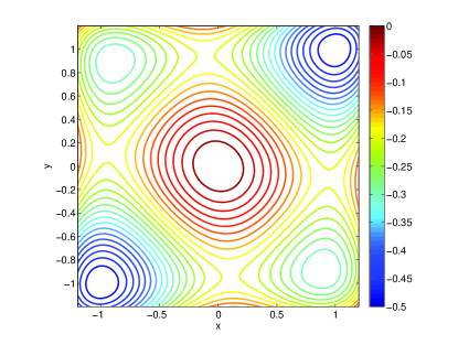
Figure 2: (Color) A contour plot of the potential function $V(x,y;0.1)$.

The system has stable equilibria at $(x,y)=(-1,-1)$ and $(1,1)$. The equilibrium solution $(x,y)=(0,0)$ is unstable for $K<1/2$ and a saddle point for $K>1/2$. For $K\leq 1/2$, the symmetric configuration about $0$, with $(x,y)=(\pm\sqrt{1-2K},\mp\sqrt{1-2K})$, is stable for $K\in[0,1/3)$ and a saddle for $K\in(1/3,1/2]$. As $K\rightarrow 1/2^{-}$, this solution approaches the unstable equilibrium at $(0,0)$. The solutions collide at $K=1/2$, resulting in a saddle point at $(0,0)$.

The system has 4 additional equilibria, defined by

$$(x,y)=(\zeta,\frac{\zeta}{K}(\zeta^{2}+K-1))$$ (28)

where $\zeta$ is a root of

$$\zeta^{4}+(K-1)\zeta^{2}+K^{2}=0.$$ (29)

Solutions exist for $K\in[0,1/3]$; the corresponding equilibria are saddle points. A plot of the equilibria for this system for different $K$ is shown in Fig. 3.

Figure 3: (Color) Values of zeroes of the deterministic vector field as a function of the coupling strength $K$. The solid black lines denotes a solutions to the exact expression in Eq. 28, showing the location of a saddle point $(x_{s},y_{s})$ of the system. Dashed lines denote the asymptotic approximate of the saddle point location for $K\ll 1$. Solid colored lines denote the location of the attractor $(x_{a},y_{a})$. Blue and red are used to denote the positions of $\bar{x}$ and $\bar{y}$, respectively, where $\bar{x}=x_{a}$ or $x_{s}$ and $\bar{y}=y_{a}$ or $y_{s}$.

III.2 Switching

When adding noise into the system, it is possible to observe noise-induced switching between stable equilibria of the noise-free system. Here we will derive most-likely noise-induced switching paths starting from the stable symmetric configuration where the particles are located in separate basins; $x$ then experiences a large fluctuation and transitions to the basin occupied by $y$. In the small-noise limit, the most likely path passes through a saddle point of the noise-free system. In the following analysis, we therefore compute the optimal switching path from the initial system configuration to the saddle point; the remaining transition from the saddle to the final stable configuration occurs much more rapidly, since it is dominated by the deterministic dynamics.

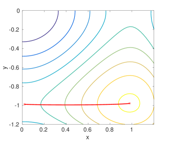
Figure 4: (Color) The potential function Eq. 27 for $K=0.0209$ for the zero noise case. Overlaid is the predicted optimal path (red line) computed when $\epsilon=\frac{1}{2}$. For the boundary conditions chosen, $x$ starts near 1 and goes through a large fluctuation, while $y$ remains approximately stationary near -1.

For sufficiently small noise intensity $D$, the switching dynamics can be described using the Hamiltonian formulation of Eq. 12, where we extend the system to 4 dimensions by adding in conjugate momenta ($\lambda_{1}$ and $\lambda_{2}$), and set the multiplicative noise terms to the identity:

$$\dot{x} =f(x)-K\cdot(x-y)+2\epsilon^{2}\lambda_{1}$$ (30a)

$$\dot{y} =f(y)+K\cdot(x-y)+2\lambda_{2}$$ (30b)

$$\dot{\lambda}_{1} =-(f^{\prime}(x)-K)\lambda_{1}-K\lambda_{2}$$ (30c)

$$\dot{\lambda}_{2} =-(f^{\prime}(y)-K)\lambda_{2}-K\lambda_{1},$$ (30d)

with corresponding Hamiltonian

$$\mathcal{H}(x,y,\lambda_{1},\lambda_{2}) =[f(x)-K\cdot(x-y)]\lambda_{1}$$ (31)

$$+[f(y)+K\cdot(x-y)]\lambda_{2}+\lambda_{2}^{2}+\epsilon^{2}\lambda_{1}^{2}.$$

Note that $\mathcal{H}(x^{*},y^{*},0,0)=0$ for all $(x^{*},y^{*})$ in the set of equilibria of (26). Since $\mathcal{H}$ is time-invariant, optimal switching paths between equilibria are required to satisfy a two-point boundary problem on the zero level sets of $\mathcal{H}=0$ in order to compute the action.

We use the numerical approach described in Lindley and Schwartz (2013) to compute the optimal path starting at $(x_{a},y_{a})=(\sqrt{1-2K},-\sqrt{1-2K})$ for $t\rightarrow-\infty$ and passing through the saddle point given by $(x_{s},y_{s})=(\zeta,\frac{\zeta}{K}(\zeta^{2}+K-1))\approx(K+K^{2}/2,-1+2K+5K^{2}/8)$ as $t\rightarrow\infty$, where $1/\sqrt{3}<\zeta<1$, and $K\ll 1$. An example of such a path is shown in Fig. 4.

In Eqs. 30, consider the limit $K\rightarrow 0$. The particle motions are uncoupled, and the situation is equivalent to a single-particle switching problem. In this case, it is possible to find an analytic solution in time explicitly, and make use of the general perturbation theory. From Eq. 24, we know that for non-zero $\epsilon$, the zeroth order term of the action scales inversely with $\epsilon^{2}$, and in fact is given by

$$R^{0}=\frac{1}{4\epsilon^{2}},$$ (32)

where we have used the fact that from the Hamiltonian, the optimal path when $K=0$ is given explicitly by $\lambda_{1}^{0}=-\frac{1}{\epsilon^{2}}f(x^{0})$.

To get the first order corrections, we need the solution to the two point value problem along the zeroth order optimal path as a function of time:

$$x^{0}(t) =\frac{1}{\sqrt{1+e^{2t}}}$$ (33a)

$$y^{0}(t) =-1$$ (33b)

$$\lambda_{1}^{0}(t) =-{\frac{{{\rm e}^{2\,t}}}{\left(1+{{\rm e}^{2\,t}}\right)^{3/2}{\epsilon}^{2}}}$$ (33c)

$$\lambda_{2}^{0}(t) =0$$ (33d)

Notice that as $t\rightarrow\pm\infty$, we have the following boundary conditions satisfied for $(x^{0}(t),\lambda_{1}^{0}(t))$ while holding $(y^{0}\equiv-1,\lambda_{2}^{0}=0)$ constant:

$$\lim_{t\rightarrow-\infty} \lim_{t\rightarrow\infty}$$

$$x^{0}(t) \rightarrow x_{a}^{0}=1 x^{0}(t) \rightarrow x_{s}^{0}=0$$ (34a)

$$\lambda_{1}^{0}(t) \rightarrow 0 \lambda_{1}^{0}(t) \rightarrow 0.$$ (34b)

Using the zeroth order time series in the first order expression of the action gives, to linear order in $K$:

$${\cal R}=\frac{1}{4\epsilon^{2}}-K\frac{3}{2\epsilon^{2}}.$$ (35)

III.3 Second order effects

We can get the second order effects of the coupling strength $K$ on the action by considering the potential function of Eq. 27, and using the general results of computing the probability of escape for Gaussian noise in Bouchet and Reygner (2016). However, the approach here is one that will be problem-specific. We choose to formally examine the Hamiltonian in Eq. 31, and notice that $y$ and its conjugate momenta remain approximately near the attractor. Therefore, we use the asymptotic expression of the attractor and saddle, in the limits of Eq. 22.

$$\mathcal{R}_{1} =\int_{-\infty}^{\infty}dt[\bm{\lambda_{1}}(t)\cdot\hat{{\bf h}}_{1}(\bm{x}(t),\bm{y}(t))$$ (36)

$$\quad\quad\quad+\bm{\lambda_{2}}(t)\cdot\hat{{\bf h}}_{2}(\bm{x}(t),\bm{y}(t))]$$

$$=-\int_{-\infty}^{\infty}dt\frac{f(x_{0}(t)}{\epsilon^{2}}(x_{0}(t)-y_{0}(t))$$

$$=\frac{1}{\epsilon^{2}}\int_{x_{a}(K)}^{x_{s}(K)}dx_{0}(x_{0}+1)$$

Using the asymptotic expressions for the attractor and saddle for $x_{0}$, expanding for small $K$, and collecting terms, we have

$${\cal R}\approx\frac{1}{4\epsilon^{2}}-\frac{3K}{2\epsilon^{2}}+\frac{2{K}^{2}}{\epsilon^{2}}.$$ (37)

An example of the optimal path projections is given in Fig. 5 for moderate noise reduction ($\epsilon=0.5$) and small coupling $K$. Notice that in the figure, $(x(t),y(t))$ spend most of their time near the equilibria specified at the boundaries. In addition, $x(t)$ traverses a distance of order unity when it switches from the attractor to the saddle point, while deviations of $y(t)$ from the equilibrium position are only of order $K$. Therefore, even though the scaled reduction of the noise parameter is small, the noise transmitted to $x$ has a very strong effect through the coupling.

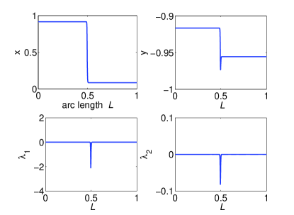
Figure 5: (Color) Trajectory projections of the optimal path where time is rescaled to be arc length, L, along the trajectory. Shown are trajectories for $x,y$ and their conjugate variables $\lambda_{1},\lambda_{2}$. The parameters used are $\epsilon=0.5,K=0.08$.

Using the theory for the action, Fig. 6 shows how it scales as a function of $K$ when $\epsilon=0.5$. Along with the numerically computed action are the results from the asymptotic analysis for small coupling using Eq. 37. Notice that for $K<0.2$, the agreement is good, and improves as $K$ gets smaller.

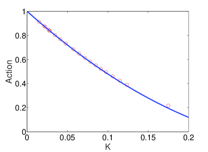
Figure 6: (Color) The numerically computed action (red circles) plotted as a function of coupling parameter $K$, for $\epsilon=0.5$. The asymptotic result for small $K$ obtained using Eq. 37 is shown by the blue curve.

One of the interesting facets of the problem occurs when there is noise only on the $y$ component. This situation occurs when $\epsilon$ approaches zero. Although asymptotically the action is seen to approach $\infty$ as $\epsilon$ approaches zero, since the system is coupled it is possible to compute an optimal path conditioned on that large fluctuations occur only in $x$. Using the results for finite $\epsilon$ as an initial guess, we use continuation to decrease $\epsilon$ to $0$, and obtain the optimal path for switching in the coupled system with noise acting only on particle $y$ (see Fig. 7), where the coupling constant is relatively small; i.e. $K\approx 0.06$. The action along the optimal path is on the order of $10^{5}$, which indicates that switching would be an extremely rare event. In this case we do observe a relatively large change in $y$ which is on the order of unity rather than $K$, but $y$ does spend most its time near its equilibrium.

The interaction of the coupling and noise induced forces is key in determining the switching times for the system. Increasing the coupling $K$ by an order of magnitude results in a drastic change in the values of the conjugate variables along the optimal switching path, as shown in Fig. 7-8. Here we see that in the system with increased $K$ (Fig. 8), both $x$ and $y$ still undergo a change of order unity; however, the values of the conjugate variables $\lambda_{1},\lambda_{2}$, have been reduced by several orders of magnitude. The action is therefore much smaller (${\cal R}\approx 500$ compared to ${\cal R}\approx 5.7\cdot 10^{5}$ with weak coupling), implying a much shorter switching time.

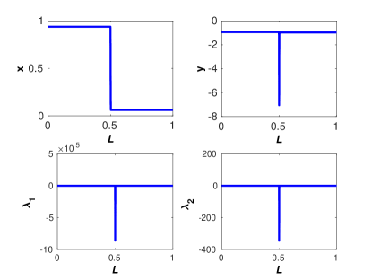
Figure 7: (Color) Optimal switching path for the system in (30), with $K=0.0595$ and $\epsilon=0$ to machine precision.

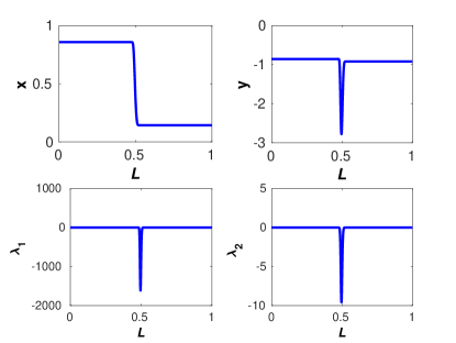
Figure 8: (Color) Trajectory projections of the optimal path where time is rescaled to be arc length, L, along the trajectory. Shown are trajectories for $x,y$ and their conjugate variables $\lambda_{1},\lambda_{2}$. The parameters used are $\epsilon=0.0,K=0.1324$.

The effect of coupling strength on action along the optimal path is shown in Fig. 9, for different values of $\epsilon$. We observe that the range of $K$ for which the asymptotic prediction ($K\ll 1$) of the action holds decreases as $\epsilon$ decreases.

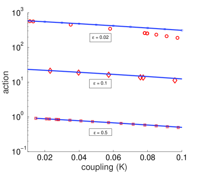
Figure 9: (Color) A plot showing the numerically computed log of the action and the asymptotic approximation (Eq. 37) as a function of coupling strength, $K$. Shown are results for $\epsilon=0.5,0.1,0.02$. The computed action is shown in red, while the asymptotic expression is depicted by the blue lines.

III.4 Monte Carlo Simulation

We consider the problem of switching in Eqs. 26 where the asymmetry in noise intensity between two coupled systems is governed by the parameter $\epsilon$. Using the Milstein method for numerical solution of stochastic differential equations (SDEs), we implement a Monte Carlo scheme to compute the mean time for the $x$ variable to switch while the $y$ variable remains in its basin, given that the particles start in different basins of attraction. That is, we compute the mean time it takes for $x$ to transition from $x(0)=x_{a}(K)$ to the saddle point $x(T)=x_{s}(K)$.

We first check the existence of an exponential distribution of times by computing the switching time as a function of the inverse noise intensity for various values of $\epsilon$ and $K$. From the ansatz that the mean switching time exponents are proportional to ${\cal R}/D$, we plot the log of the mean switching time as a function of $1/D$, where the slope should be the action evaluated at the parameters of $\epsilon,K$.

We can see how the asymptotic theory holds as a function of $K$ by comparing it with the mean switching times in Figs. 10-11. For small $K$, the theory holds up quite well for a range of noise intensities (where noise intensity is small compared to the barrier height), and over sufficiently large range of $K$.

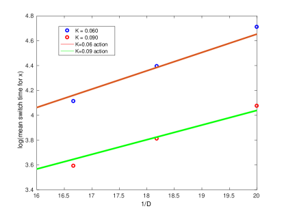
Figure 10: (Color) Plotted is the mean switching time for $x$ to go from the attractor to the saddle point while $y$ remains in its basin of attraction, as a function of inverse noise intensity ($1/D$). Here $\epsilon=0.75$. Results are shown for $K=0.060$ and $0.090$. The solid lines show theoretical values computed using Eq. 30, while values obtained from Monte Carlo simulations are depicted by circles.

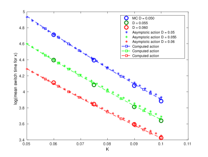
Figure 11: (Color) Plotted is the mean switching time for $x$ as a function of coupling strength $K$. Here $\epsilon=0.75$. Results for $D=0.050$, $0.055$, and $0.060$ are shown in blue, green, and red, respectively. Values obtained from Monte Carlo simulations are plotted as circles; values computed using the asymptotic theory (Eq. 37) are plotted as stars; and true values for the action are plotted as dashed lines. Since the prefactor is not directly computed in the asymptotic calculations of action, the plotted values are shifted to coincide with the first data point. Note that the asymptotic values deviate from the true values for large K.

IV Discussion and Conclusion

In this paper, we addressed the problem of how coupling can enhance noise-induced switching in systems with highly asymmetric noise characteristics. As a motivating example, we considered a simple mixed-reality experiment in which a virtual system with very low or zero noise is coupled with a noisy real system. We showed that the effect of coupling was sufficient to cause the virtual dynamics to undergo a large fluctuation while the real dynamics, which was driven by larger noise intensity, remained quiescent. It was very natural to take a variational approach to describing such a large fluctuation, and although it was applied to Gaussian noise, the same approach can be extended to more general noise sources Billings et al. (2010).

Using the variational approach, we generated a Hamiltonian two-point boundary value problem with asymmetric driving representing the effect of the heterogeneous noise sources. We used scaling parameter $\epsilon\in[0,1]$ to quantify the asymmetry in the noise. The solution to the Hamiltonian equations generates the optimal switching path, which in turn can be used to predict mean switching rates.

We focused on the case where a large fluctuation occurs in the low noise system, while the system with higher intensity noise remains near its equilibrium point. Note that, because of the asymmetry in noise levels, the probability of a large transition in the high noise system occurring before the fluctuation in the low noise system is very high. Thus having the low noise system transition first is an extremely rare event.

We illustrated the general theory using a general model of a pair of coupled particles in a bi-stable potential. This example was inspired by bistable behaviors predicted for a mixed-reality system of swarming agents Szwaykowska et al. (2016a). We quantified the action as a function of coupling strength over a range of scaling values $\epsilon$, revealing an excellent comparison between asymptotic theory and numerical solutions of the optimal paths. However, we note that, for very small values of $\epsilon$, the asymptotic theory diverges from the true action for even moderate values of $K$. This is a result of two small parameters in the approximation; higher-order corrections may need to be included in Eq. 37. We also quantified the mean escape times in terms of parameters $\epsilon$ and $D$, again with excellent agreement between simulation and theory for the log of the mean switching time.

We computed the paths as the noise scaling parameter $\epsilon$ approaches zero, so that the probability of extremely rare events is governed by coupling strength alone. That is, the noise is only transmitted through the coupling terms. The asymptotic theory predicts an logarithmic exponent of the probability of virtual switching given that the real dynamics exhibits only small fluctuations, where the exponent scales as $1/\epsilon^{2}$. Although extremely rare, the switching is still observed when $\epsilon\rightarrow 0$ and coupling $K$ is sufficiently large Meerson , as we have shown in Fig. 8.

The physical interpretation of the transmitted noise induced large fluctuation is that the coupling also acts as an effective force along with the effective stochastic momenta to enhance the observation of an extremely rare event. The coupling used in the generic example is similar to the couplings found in many physical systems, including the swarm experiment we described. Since our theory is generic, it predicts that such noise transmitted fluctuations should appear in many coupled systems, including mixed-reality situations, where the noise intensities are highly skewed.

V Acknowledgments

The authors gratefully acknowledge the Office of Naval Research for their support under N0001412WX20083, and support of the NRL Base Research Program N0001412WX30002. KS was a National Research post doctoral fellow while performing the research. We acknowledge useful conversations with Ani Hsieh, Luis Mier, and Brandon Lindley about early versions of the research, and Jason Hindes for an initial reading of the manuscript.

References

- Gardiner (2004) C. W. Gardiner, Handbook of Stochastic Methods for Physics, Chemistry and the Natural Sciences (Springer-Verlag, 2004).
- Van Kampen (2007) N. G. Van Kampen, Stochastic Processes in Physics and Chemistry (Elsevier, 2007).
- Freidlin and Wentzell (1984) M. I. Freidlin and A. D. Wentzell, Random Perturbations of Dynamical Systems (Springer-Verlag, 1984).
- Doering and Gadoua (1992) C. R. Doering and J. C. Gadoua, Phys. Rev. Lett. 69, 2318 (1992).
- Castellano et al. (1996) M. G. Castellano, G. Torrioli, C. Cosmelli, A. Costantini, F. Chiarello, P. Carelli, G. Rotoli, M. Cirillo, and R. L. Kautz, Phys. Rev. B 54, 15417 (1996).
- Lapidus et al. (1999) L. J. Lapidus, D. Enzer, and G. Gabrielse, Phys. Rev. Lett. 83, 899 (1999).
- Kim et al. (2005) K. Kim, M. S. Heo, K. H. Lee, H. J. Ha, K. Jang, H. R. Noh, and W. Jhe, Phys. Rev. A 72, 053402 (2005).
- Siddiqi et al. (2005) I. Siddiqi, R. Vijay, F. Pierre, C. M. Wilson, L. Frunzio, M. Metcalfe, C. Rigetti, R. J. Schoelkopf, M. H. Devoret, D. Vion, and D. Esteve, Phys. Rev. Lett. 94, 027005 (2005).
- Chan and Stambaugh (2007) H. B. Chan and C. Stambaugh, Phys. Rev. Lett. 99, 060601 (2007).
- Dykman and Schwartz (2012) M. I. Dykman and I. B. Schwartz, PHYSICAL REVIEW E 86 (2012), 10.1103/PhysRevE.86.031145.
- D’Huys et al. (2014) O. D’Huys, T. Juengling, and W. Kinzel, PHYSICAL REVIEW E 90 (2014), 10.1103/PhysRevE.90.032918.
- Emenheiser et al. (2016) J. Emenheiser, A. Chapman, M. Posfai, J. P. Crutchfield, M. Mesbahi, and R. M. D’Souza, CHAOS 26 (2016), 10.1063/1.4960191.
- Huang et al. (2016) Q. Huang, C. Xue, and J. Tang, AIP Adv. 6, 015219 (2016).
- Allen et al. (2005) R. J. Allen, P. B. Warren, and P. R. Ten Wolde, Phys. Rev. Lett. 94 (2005), 10.1103/PhysRevLett.94.018104, arXiv:0406006 [q-bio] .
- Barzel and Biham (2008) B. Barzel and O. Biham, Phys. Rev. E - Stat. Nonlinear, Soft Matter Phys. 78, 1 (2008).
- Kamenev et al. (2008) A. Kamenev, B. Meerson, and B. Shklovskii, Phys. Rev. Lett. 101, 268103 (2008).
- Kamenev and Meerson (2008) A. Kamenev and B. Meerson, Phys. Rev. E 77, 061107 (2008).
- Dykman et al. (2008) M. I. Dykman, I. B. Schwartz, and A. S. Landsman, Phys. Rev. Lett. 101, 078101 (2008).
- Wells et al. (2015) D. K. Wells, W. L. Kath, and A. E. Motter, PHYSICAL REVIEW X 5 (2015), 10.1103/PhysRevX.5.031036.
- Chen et al. (2016) H. Chen, P. Thill, and J. Cao, J. Chem. Phys. 144 (2016), 10.1063/1.4948461.
- Hindes and Schwartz (2016) J. Hindes and I. B. Schwartz, Phys. Rev. Lett. 117, 028302 (2016).
- Schwartz et al. (2011) I. Schwartz, E. Forgoston, S. Bianco, and L. Shaw, Journal of The Royal Society Interface 8, 1699 (2011).
- Dykman (1990) M. I. Dykman, Phys. Rev. A 42, 2020 (1990).
- Le Masne et al. (2009) Q. Le Masne, H. Pothier, N. O. Birge, C. Urbina, and D. Esteve, PHYSICAL REVIEW LETTERS 102 (2009), 10.1103/PhysRevLett.102.067002.
- Ankerhold and Pechukas (1999) J. Ankerhold and P. Pechukas, JOURNAL OF CHEMICAL PHYSICS 111, 4886 (1999).
- Lindley et al. (2013) B. S. Lindley, L. Mier-y-Teran Romero, and I. B. Schwartz, in 2013 American Control Conference (Ieee, 2013) pp. 4587–4591.
- Earon et al. (2001) E. Earon, T. Barfoot, and G. D’Eleuterio (2001) pp. 1267–1272, IEEE/ASME International Conference on Advanced Intelligent Mechatronics.
- Benerjee and Deepthi (2015) C. Benerjee and N. Deepthi (2015) pp. 1–6, International Conference on Robotics, Automation, Control and Embedded Systems.
- Bhattacharya et al. (2012) S. Bhattacharya, R. Ghrist, and V. Kumar, International Journal of Robotics Research 33, 113 (2012).
- Lynch et al. (2008) K. M. Lynch, I. B. Schwartz, P. Yang, and R. A. Freeman, IEEE Transactions on Robotics 24, 710 (2008).
- Wu and Zhang (2011) W. Wu and F. Zhang, Automatica 47, 2044 (2011).
- Takano et al. (2014) R. Takano, D. Yamazaki, Y. Ichikawa, K. Hattori, and K. Takadama (2014) pp. 585 – 590, IEEE International Conference on Systems, Man and Cybernetics.
- Al Tair et al. (2015) H. Al Tair, T. Taha, M. Al-Qutayri, and J. Dias (2015) pp. 210–213, International Conference on Information and Communication Technology Research.
- Augugliaro et al. (2014) F. Augugliaro, S. Lupashin, M. Hamer, C. Male, M. Hehn, M. W. Mueller, J. S. Willmann, F. Gramazio, M. Kohler, and R. D’Andrea, IEEE Control Systems 34, 46 (2014).
- Ramp et al. (2009) S. R. Ramp, R. E. Davis, N. E. Leonard, I. Shulman, Y. Chao, A. R. Robinson, J. E. Marsden, P. F. J. Lermusiaux, D. M. Fratantoni, J. D. Paduan, F. P. Chavez, F. L. Bahr, S. Liang, W. Leslie, and Z. Li, Deep Sea Research Part II: Topical Studies in Oceanography 56, 68 (2009).
- Dorigo et al. (2013) M. Dorigo, D. Floreano, L. M. Gambardella, F. Mondada, S. Nolfi, T. Baaboura, M. Birattari, M. Bonani, M. Brambilla, A. Brutschy, D. Burnier, A. Campo, A. L. Christensen, A. Decugniere, G. Di Caro, F. Ducatelle, E. Ferrante, A. Forster, J. M. Gonzales, J. Guzzi, V. Longchamp, S. Magnenat, N. Mathews, M. Montes de Oca, R. O’Grady, C. Pinciroli, G. Pini, P. Retornaz, J. Roberts, V. Sperati, T. Stirling, A. Stranieri, T. Stutzle, V. Trianni, E. Tuci, A. E. Turgut, and F. Vaussard, IEEE Robotics & Automation Magazine 20, 60 (2013).
- Szwaykowska et al. (2016a) K. Szwaykowska, I. B. Schwartz, L. M.-y.-T. Romero, C. R. Heckman, D. Mox, and M. A. Hsieh, Physical Review E 93, 032307 (2016a).
- Hindes et al. (2016) J. Hindes, K. Szwaykowska, and I. B. Schwartz, PHYSICAL REVIEW E 94, 032306 (2016).
- Ben-Jacob et al. (1997) E. Ben-Jacob, I. Cohen, A. Czirók, T. Vicsek, and D. L. Gutnick, Physica A 238, 181 (1997).
- Calovi et al. (2014) D. S. Calovi, U. Lopez, S. Ngo, C. Sire, H. Chaté, and G. Theraulaz, New Journal of Physics 16, 015026 (2014), arXiv:1308.2889 .
- Carlen et al. (2013) E. Carlen, R. Chatelin, P. Degond, and B. Wennberg, Physica D: Nonlinear Phenomena 260, 90 (2013).
- Hsieh et al. (2008) M. A. Hsieh, Á. Halász, S. Berman, and V. Kumar, Swarm Intelligence 2, 121 (2008).
- Gintautas and Hübler (2007) V. Gintautas and A. W. Hübler, Phys. Rev. E 75, 057201 (2007).
- Szwaykowska et al. (2016b) K. Szwaykowska, I. B. Schwartz, L. Mier-y Teran-Romero, C. R. Heckman, D. Mox, and M. A. Hsieh, Physical Review E 93, 032307 (2016b).
- Kozlov et al. (2016) V. Kozlov, S. Vakulenko, and U. Wennergren, Phys. Rev. E 93, 1 (2016).
- Dykman (2010) M. I. Dykman, Phys. Rev. E 81, 051124 (2010).
- Feynman and Hibbs (1965a) R. P. Feynman and A. R. Hibbs, Quantum Mechanics and Path Integrals (McGraw-Hill, Inc., 1965).
- Note (1) Throughout the paper, boldface lower-case letters will indicate vectors, while boldface upper-case letters will indicate matrices.
- Fleming and Rishel (1975) W. Fleming and R. Rishel, Deterministic and stochastic optimal control (Springer New York, 1975).
- Note (2) The vector multiplication here is assumed to be an inner product.
- Feynman and Hibbs (1965b) R. P. Feynman and A. R. Hibbs, Quantum Mechanics and Path Integrals (McGraw-Hill, New-York, 1965).
- Lindley and Schwartz (2013) B. S. Lindley and I. B. Schwartz, Physica D: Nonlinear Phenomena 255, 22 (2013).
- Bouchet and Reygner (2016) F. Bouchet and J. Reygner, Annales Henri Poincaré 17, 3499 (2016).
- Billings et al. (2010) L. Billings, I. B. Schwartz, M. McCrary, A. N. Korotkov, and M. I. Dykman, Phys. Rev. Lett. 104, 140601 (2010).
- (55) B. Meerson, Private communication.