New Physics in $b\to s\mu^{+}\mu^{-}$: Distinguishing Models through CP-Violating Effects

Abstract

At present, there are several measurements of $B$ decays that exhibit discrepancies with the predictions of the SM, and suggest the presence of new physics (NP) in $b\to s\mu^{+}\mu^{-}$ transitions. Many NP models have been proposed as explanations. These involve the tree-level exchange of a leptoquark (LQ) or a flavor-changing $Z^{\prime}$ boson. In this paper we examine whether it is possible to distinguish the various models via CP-violating effects in $B\to K^{(*)}\mu^{+}\mu^{-}$. Using fits to the data, we find the following results. Of all possible LQ models, only three can explain the data, and these are all equivalent as far as $b\to s\mu^{+}\mu^{-}$ processes are concerned. In this single LQ model, the weak phase of the coupling can be large, leading to some sizeable CP asymmetries in $B\to K^{(*)}\mu^{+}\mu^{-}$. There is a spectrum of $Z^{\prime}$ models; the key parameter is $g_{L}^{\mu\mu}$, which describes the strength of the $Z^{\prime}$ coupling to $\mu^{+}\mu^{-}$. If $g_{L}^{\mu\mu}$ is small (large), the constraints from $B^{0}_{s}$-${\bar{B}}^{0}_{s}$ mixing are stringent (weak), leading to a small (large) value of the NP weak phase, and corresponding small (large) CP asymmetries. We therefore find that the measurement of CP-violating asymmetries in $B\to K^{(*)}\mu^{+}\mu^{-}$ can indeed distinguish among NP $b\to s\mu^{+}\mu^{-}$ models.

I Introduction

At present, there are several measurements of $B$ decays involving $b\to s\ell^{+}\ell^{-}$ that suggest the presence of physics beyond the standard model (SM). These include

1. $B\to K^{*}\mu^{+}\mu^{-}$: Measurements of $B\to K^{*}\mu^{+}\mu^{-}$ have been made by the LHCb BK*mumuLHCb1 ; BK*mumuLHCb2 and Belle BK*mumuBelle Collaborations. They find results that deviate from the SM predictions. The main discrepancy is in the angular observable $P^{\prime}_{5}$ P'5 . Its significance depends on the assumptions made regarding the theoretical hadronic uncertainties BK*mumuhadunc1 ; BK*mumuhadunc2 ; BK*mumuhadunc3 . The latest fits to the data Altmannshofer:2014rta ; BK*mumulatestfit1 ; BK*mumulatestfit2 take into account the hadronic uncertainties, and find that a significant discrepancy is still present, perhaps as large as $\sim 4\sigma$.

2. $B^{0}_{s}\to\phi\mu^{+}\mu^{-}$: The LHCb Collaboration has measured the branching fraction and performed an angular analysis of $B^{0}_{s}\to\phi\mu^{+}\mu^{-}$ BsphimumuLHCb1 ; BsphimumuLHCb2 . They find a $3.5\sigma$ disagreement with the predictions of the SM, which are based on lattice QCD latticeQCD1 ; latticeQCD2 and QCD sum rules QCDsumrules .

3. $R_{K}$: The ratio $R_{K}\equiv{\cal B}(B^{+}\to K^{+}\mu^{+}\mu^{-})/{\cal B}(B^{+}\to K^{+}e^{+}e^{-})$ has been measured by the LHCb Collaboration in the dilepton invariant mass-squared range 1 GeV² $\leq q^{2}\leq 6$ GeV² RKexpt , with the result

   $$R_{K}^{\rm expt}=0.745^{+0.090}_{-0.074}~{}{\rm(stat)}\pm 0.036~{}{\rm(syst)}~{}.$$ (1)

   This differs from the SM prediction of $R_{K}^{\rm SM}=1\pm 0.01$ IsidoriRK by $2.6\sigma$, and thus is a hint of lepton flavor non-universality.

While any suggestions of new physics (NP) are interesting, what is particularly intriguing about the above set of measurements is that they can all be explained if there is NP in $b\to s\mu^{+}\mu^{-}$. To be specific, $b\to s\mu^{+}\mu^{-}$ transitions are defined via the effective Hamiltonian

$$H_{\rm eff} = -\frac{\alpha G_{F}}{\sqrt{2}\pi}V_{tb}V_{ts}^{*}\sum_{a=9,10}(C_{a}O_{a}+C^{\prime}_{a}O^{\prime}_{a})~{},$$

$$O_{9(10)} = [{\bar{s}}\gamma_{\mu}P_{L}b][{\bar{\mu}}\gamma^{\mu}(\gamma_{5})\mu]~{},$$ (2)

where the $V_{ij}$ are elements of the Cabibbo-Kobayashi-Maskawa (CKM) matrix. The primed operators are obtained by replacing $L$ with $R$, and the Wilson coefficients (WCs) $C^{(\prime)}_{a}$ include both SM and NP contributions. Global analyses of the $b\to s\ell^{+}\ell^{-}$ anomalies have been performed Descotes-Genon:2013wba ; Altmannshofer:2014rta ; BK*mumulatestfit1 ; BK*mumulatestfit2 . It was found that there is a significant disagreement with the SM, possibly as large as $4\sigma$, and it can be explained if there is NP in $b\to s\mu^{+}\mu^{-}$. Ref. BK*mumulatestfit1 gave four possible explanations: (I) $C_{9}^{\mu\mu}({\rm NP})<0$, (II) $C_{9}^{\mu\mu}({\rm NP})=-C_{10}^{\mu\mu}({\rm NP})<0$, (III) $C_{9}^{\mu\mu}({\rm NP})=-C_{9}^{\prime\mu\mu}({\rm NP})<0$, (IV) $C_{9}^{\mu\mu}({\rm NP})=-C_{10}^{\mu\mu}({\rm NP})=-C_{9}^{\prime\mu\mu}({\rm NP})=-C_{10}^{\prime\mu\mu}({\rm NP})<0$.

Numerous models have been proposed that generate the correct NP contribution to $b\to s\mu^{+}\mu^{-}$ at tree level. Most of them use solution (II) above, though a few use solution (I). These models can be separated into two categories: those containing leptoquarks (LQs) CCO ; AGC ; HS1 ; GNR ; VH ; SM ; FK ; BFK ; BKSZ , and those with a $Z^{\prime}$ boson CCO ; Crivellin:2015lwa ; Isidori ; dark ; Chiang ; Virto ; GGH ; BG ; BFG ; Perimeter ; CDH ; SSV ; CHMNPR ; CMJS ; BDW ; FNZ ; AQSS ; CFL ; Hou ; CHV ; CFV ; CFGI ; IGG ; BdecaysDM ; Bhatia:2017tgo . But this raises an obvious question: assuming that there is indeed NP in $b\to s\mu^{+}\mu^{-}$, which model is the correct one? In other words, short of producing an actual LQ or $Z^{\prime}$ experimentally, is there any way of distinguishing the models?

A first step was taken in Ref. RKRDmodels , where it was shown that the CP-conserving, lepton-flavor-violating decays $\Upsilon(3S)\to\mu\tau$ and $\tau\to 3\mu$ are useful processes for differentiating between LQ and $Z^{\prime}$ models. In the present paper, we compare the predictions of the various models for CP-violating asymmetries in $B\to K^{*}\mu^{+}\mu^{-}$ and $B\to K\mu^{+}\mu^{-}$.

CP-violating effects require the interference of two amplitudes with a relative weak (CP-odd) phase. (For certain CP-violating effects, a relative strong (CP-even) phase is also required.) In the SM, $b\to s\mu^{+}\mu^{-}$ is dominated by a single amplitude, proportional to $V_{tb}V_{ts}^{*}$ [see Eq. (2)]. In order to generate CP-violating asymmetries, it is necessary that the NP contribution to $b\to s\mu^{+}\mu^{-}$ have a sizeable weak phase. As we will see, this does not hold in all NP models, so that CP-violating asymmetries in $B\to K^{*}\mu^{+}\mu^{-}$ and $B\to K\mu^{+}\mu^{-}$ can be a powerful tool for distinguishing the models. (The usefulness of CP asymmetries in $B\to K^{*}\mu^{+}\mu^{-}$ for identifying NP was also discussed in Ref. BHP .)

We perform both model-independent and model-dependent analyses. In the model-independent case, we assume that the NP contributes to a particular set of WCs (and we consider several different sets). But if a particular model is used, one can work out which WCs are affected. In either case, a fit to the data is performed to establish (i) whether a good fit is obtained, and (ii) what are the best-fit values and allowed ranges of the real and imaginary pieces of the WCs. In the case of a good fit, the predictions for CP-violating asymmetries in $B\to K^{*}\mu^{+}\mu^{-}$ and $B\to K\mu^{+}\mu^{-}$ are computed.

The data used in the fits include all CP-conserving observables involving $b\to s\mu^{+}\mu^{-}$ transitions. The processes are $B^{0}\to K^{*0}(\to K^{+}\pi^{-})\mu^{+}\mu^{-}$, $B^{+}\to K^{*+}\mu^{+}\mu^{-}$, $B^{+}\to K^{+}\mu^{+}\mu^{-}$, $B^{0}\to K^{0}\mu^{+}\mu^{-}$, $B^{0}_{s}\to\phi\mu^{+}\mu^{-}$, $B\to X_{s}\mu^{+}\mu^{-}$, and $B^{0}_{s}\to\mu^{+}\mu^{-}$. For the first process, a complete angular analysis of $B^{0}\to K^{*0}(\to K^{+}\pi^{-})\mu^{+}\mu^{-}$ was performed in Refs. BHP ; BK*mumuCPV . It was shown that this decay is completely described in terms of twelve angular functions. By averaging over the angular distributions of $B$ and ${\bar{B}}$ decays, one obtains CP-conserving observables. There are nine of these. Most of the observables are measured in different $q^{2}$ bins, so that there are a total of 106 CP-conserving observables in the fit.

For the model-independent fits, only the $b\to s\mu^{+}\mu^{-}$ data is used. However, for the model-dependent analyses, additional data may be taken into account. That is, in a specific model, there may be contributions to other processes such as $b\to s\nu{\bar{\nu}}$, $B^{0}_{s}$-${\bar{B}}^{0}_{s}$ mixing, etc. The choice of additional data is made on a model-by-model basis. Because the model-independent and model-dependent fits can involve different experimental (and theoretical) constraints, they may yield significantly different results.

CP-violating asymmetries are obtained by comparing $B$ and ${\bar{B}}$ decays. In the case of $B\to K\mu^{+}\mu^{-}$, there is only the direct partial rate asymmetry. For $B^{0}\to K^{*0}(\to K^{+}\pi^{-})\mu^{+}\mu^{-}$, one compares the $B$ and ${\bar{B}}$ angular distributions. This leads to seven CP asymmetries. There are therefore a total of eight CP-violating effects that can potentially be used to distinguish among the NP $b\to s\mu^{+}\mu^{-}$ models.

For the LQs, we will show that there are three models that can explain the $b\to s\mu^{+}\mu^{-}$ data. The LQs of these models contribute differently to $b\to s\nu_{\mu}{\bar{\nu}}_{\mu}$, so that, in principle, they can be distinguished by the measurements of $b\to s\nu{\bar{\nu}}$. However, the constraints from these measurements are far weaker than those from $b\to s\mu^{+}\mu^{-}$, so that all three LQ models are equivalent, as far as the $b\to s\mu^{+}\mu^{-}$ data are concerned. We find that some CP asymmetries in $B\to K^{(*)}\mu^{+}\mu^{-}$ can be large in this single LQ model.

In $Z^{\prime}$ models, there are $g_{L}^{bs}{\bar{s}}\gamma^{\mu}P_{L}bZ^{\prime}_{\mu}$ and $g_{L}^{\mu\mu}{\bar{\mu}}\gamma^{\mu}P_{L}\mu Z^{\prime}_{\mu}$ couplings, leading to a tree-level $Z^{\prime}$ contribution to $b\to s\mu^{+}\mu^{-}$. In order to explain the $b\to s\mu^{+}\mu^{-}$ anomalies, the product of couplings $g_{L}^{bs}g_{L}^{\mu\mu}$ must lie within a certain (non-zero) range. If $g_{L}^{\mu\mu}$ is small, $g_{L}^{bs}$ must be large, and vice-versa. The $Z^{\prime}$ also contributes at tree level to $B^{0}_{s}$-${\bar{B}}^{0}_{s}$ mixing, proportional to $(g_{L}^{bs})^{2}$. Measurements of the mixing constrain the magnitude and phase of $g_{L}^{bs}$. If $g_{L}^{bs}$ is large, the constraint on its phase is significant, so that this $Z^{\prime}$ model cannot generate sizeable CP asymmetries. On the other hand, if $g_{L}^{bs}$ is small, the constraints from $B^{0}_{s}$-${\bar{B}}^{0}_{s}$ mixing are not stringent, and large CP-violating effects are possible.

The upshot is that it may be possible to differentiate $Z^{\prime}$ and LQ models, as well as different $Z^{\prime}$ models, through measurements of CP-violating asymmetries in $B\to K^{(*)}\mu^{+}\mu^{-}$.

We begin in Sec. 2 with a description of our method for fitting the data and for making predictions about CP asymmetries. The $b\to s\mu^{+}\mu^{-}$ data used in the fits are given in the Appendix. We perform a model-independent analysis in Sec. 3. In Sec. 4, we perform model-dependent fits in order to determine the general features of the LQ and $Z^{\prime}$ models that can explain the $b\to s\mu^{+}\mu^{-}$ anomalies. We present the predictions of the various models for the CP asymmetries in Sec. 5. We conclude in Sec. 6.

II Method

The method works as follows. We suppose that the NP contributes to a particular set of $b\to s\mu^{+}\mu^{-}$ WCs. This can be done in a “model-independent” way, in the sense that no particular underlying NP model is assumed, or it can be done in the context of a specific NP model. In either case, all observables are written as functions of the WCs, which contain both SM and NP contributions. Given values of the WCs, we use flavio flavio to calculate the observables. By comparing the computed values of the observables with the data, the $\chi^{2}$ can be found. The program MINUIT James:1975dr ; James:2004xla ; James:1994vla is used to find the values of the WCs that minimize the $\chi^{2}$. It is then possible to determine whether or not the chosen set of WCs provides a good fit to the data. This is repeated for different sets of $b\to s\mu^{+}\mu^{-}$ WCs.

We are interested in NP that leads to CP-violating effects in $B\to K^{(*)}\mu^{+}\mu^{-}$. As noted in the introduction, this requires that the NP contribution to $b\to s\mu^{+}\mu^{-}$ have a weak phase. With this in mind, we allow the NP WCs to be complex (other fits generally take the NP contributions to the WCs to be real), and determine the best-fit values of both the real and imaginary parts of the WCs.

In the case where a particular NP model is assumed, the main theoretical parameters are the couplings of the NP particles to the SM fermions. At low energies, these generate four-fermion operators. The first step is therefore to determine which operators are generated in the NP model. This in turn establishes which observables are affected by the NP. The fit yields preferred values of the WCs, and these can be converted into preferred values for the real and imaginary parts of the couplings.

We note that caution is needed as regards the results of the model-independent fits. In such fits it is assumed that the NP contributes to a particular set of WCs. One might think that the results will apply to all NP models that contribute to the same WCs. However, this is not true. The point is that a particular model may have additional theoretical or experimental constraints. When these are taken into account, the result of the fit might be quite different. That is, the “model-independent” fits do not necessarily apply to all models. Indeed, in the following sections we will see several examples of this.

Finally, for those sets of WCs that provide good fits to the data, we compute the predictions for the CP-violating asymmetries in $B\to K^{*}\mu^{+}\mu^{-}$ and $B\to K\mu^{+}\mu^{-}$.

II.1 Fit

The $\chi^{2}$ is a function of the WCs $C_{i}$, and is constructed as follows:

$$\chi^{2}(C_{i})=(\mathcal{O}_{th}(C_{i})-\mathcal{O}_{exp})^{T}\,\mathcal{C}^{-1}\,(\mathcal{O}_{th}(C_{i})-\mathcal{O}_{exp})~{}.$$ (3)

Here $\mathcal{O}_{th}(C_{i})$ are the theoretical predictions for the various observables used as constraints. These predictions depend upon the WCs. $\mathcal{O}_{exp}$ are the the corresponding experimental measurements.

We include all available theoretical and experimental correlations in our fit. The total covariance matrix $\mathcal{C}$ is obtained by adding the individual theoretical and experimental covariance matrices, respectively $\mathcal{C}_{th}$ and $\mathcal{C}_{exp}$. The theoretical covariance matrix is obtained by randomly generating all input parameters and then calculating the observables for these sets of inputs flavio .The uncertainty is then defined by the standard deviation of the resulting spread in the observable values. In this way the correlations are generated among the various observables that share some common parameters flavio . Note that we have assumed $\mathcal{C}_{th}$ to be independent of the WCs. This implies that we take the SM covariance matrix to construct the $\chi^{2}$ function. As far as experimental correlations are concerned, these are only available (bin by bin) among the angular observables in $B\to K^{(*)}\mu^{+}\mu^{-}$ BK*mumuLHCb2 , and among the angular observables in $B^{0}_{s}\to\phi\mu^{+}\mu^{-}$ BsphimumuLHCb2 .

For $\chi^{2}$ minimization, we use the MINUIT library James:1975dr ; James:2004xla ; James:1994vla . The errors on the individual parameters are defined as the change in the values of the parameters that modifies the value of the $\chi^{2}$ function such that $\Delta\chi^{2}=\chi^{2}-\chi^{2}_{min}=1$. However, to obtain the $68.3\%$ and $95\%$ CL 2-parameter regions, we use $\Delta\chi^{2}$ equal to 2.3 and 6.0, respectively pdg .

The fit includes all CP-conserving $b\to s\mu^{+}\mu^{-}$ observables. These are

1. $B^{0}\to K^{*0}\mu^{+}\mu^{-}$: The CP-averaged differential angular distribution for $B^{0}\to K^{*0}(\to K^{+}\pi^{-})\mu^{+}\mu^{-}$ can be derived using Refs. P'5 ; BHP ; BK*mumuCPV ; it is given by BK*mumuLHCb2

   $$\frac{1}{d(\Gamma+\overline{\Gamma})/dq^{2}}\frac{d^{4}(\Gamma+\overline{\Gamma})}{dq^{2}d\vec{\Omega}}=\frac{9}{32\pi}\left[\frac{3}{4}(1-F_{L})\sin^{2}\theta_{K^{*}}+F_{L}\cos^{2}\theta_{K^{*}}\right.$$ (4)

   $$\hskip 8.53581pt+~{}\frac{1}{4}(1-F_{L})\sin^{2}\theta_{K^{*}}\cos 2\theta_{\ell}-F_{L}\cos^{2}\theta_{K^{*}}\cos 2\theta_{\ell}+S_{3}\sin^{2}\theta_{K^{*}}\sin^{2}\theta_{\ell}\cos 2\phi$$

   $$\hskip 8.53581pt+~{}S_{4}\sin 2\theta_{K^{*}}\sin 2\theta_{\ell}\cos\phi+S_{5}\sin 2\theta_{K^{*}}\sin\theta_{\ell}\cos\phi+\frac{4}{3}A_{FB}\sin^{2}\theta_{K^{*}}\cos\theta_{\ell}$$

   $$\hskip 8.53581pt\left.+~{}S_{7}\sin 2\theta_{K^{*}}\sin\theta_{\ell}\sin\phi+S_{8}\sin 2\theta_{K^{*}}\sin 2\theta_{\ell}\sin\phi+S_{9}\sin^{2}\theta_{K^{*}}\sin^{2}\theta_{\ell}\sin 2\phi\right]~{}.$$

   Here $q^{2}$ represents the invariant mass squared of the dimuon system, and $\vec{\Omega}$ represents the solid angle constructed from $\theta_{l},\theta_{K^{*}}$, and $\phi$. There are therefore nine observables in the decay: the differential branching ratio, $F_{L}$, $A_{FB}$, $S_{3}$, $S_{4}$, $S_{5}$, $S_{7}$, $S_{8}$ and $S_{9}$, all measured in various $q^{2}$ bins. The experimental measurements are given in Tables 6 and 7 in the Appendix.

   In the introduction it was mentioned that the main discrepancy with the SM is in the angular observable $P^{\prime}_{5}$. This is defined as P'5

   $$P^{\prime}_{5}=\frac{S_{5}}{\sqrt{F_{L}(1-F_{L})}}~{}.$$ (5)

2. The differential branching ratio of $B^{+}\to K^{*+}\mu^{+}\mu^{-}$. The experimental measurements Aaij:2014pli are given in Table 8 in the Appendix.

3. The differential branching ratio of $B^{+}\to K^{+}\mu^{+}\mu^{-}$. The experimental measurements Aaij:2014pli are given in Table 9 in the Appendix. When integrated over $q^{2}$, this provides the numerator in $R_{K}\equiv{\cal B}(B^{+}\to K^{+}\mu^{+}\mu^{-})/{\cal B}(B^{+}\to K^{+}e^{+}e^{-})$. Thus, the measurement of $R_{K}$ [Eq. (1)] is implicitly included here.

4. The differential branching ratio of $B^{0}\to K^{0}\mu^{+}\mu^{-}$. The experimental measurements Aaij:2014pli are given in Table 10 in the Appendix.

5. $B^{0}_{s}\to\phi\mu^{+}\mu^{-}$: The experimental measurements of the differential branching ratio and the angular observables BsphimumuLHCb2 are given respectively in Tables 11 and 12 in the Appendix.

6. The differential branching ratio of $B\to X_{s}\mu^{+}\mu^{-}$. The experimental measurements Lees:2013nxa are given in Table 13 in the Appendix.

7. ${\rm BR}(B^{0}_{s}\to\mu^{+}\mu^{-})=(2.9\pm 0.7)\times 10^{-9}$ Aaij:2013aka ; CMS:2014xfa .

In computing the theoretical predictions for the above observables, we note the following:

• For $B\to K^{*}\mu^{+}\mu^{-}$ and $B^{0}_{s}\to\phi\mu^{+}\mu^{-}$, we use the form factors from the combined fit to lattice and light-cone sum rules (LCSR) calculations QCDsumrules . These calculations are applicable to the full $q^{2}$ kinematic region. In LCSR calculations the full error correlation matrix is used, which is useful to avoid an overestimate of the uncertainties.

• In $B\to K\mu^{+}\mu^{-}$, we use the form factors from lattice QCD calculations Bailey:2015dka , in which the main sources of uncertainty are from the chiral-continuum extrapolation and the extrapolation to low $q^{2}$. In order to cover the entire kinematically-allowed range of $q^{2}$, we use the model-independent $z$ expansion given in Ref. Bailey:2015dka .

• The decay $B^{0}_{s}\to\phi\mu^{+}\mu^{-}$ has special characteristics, namely (i) there can be (time-dependent) indirect CP-violating effects, and (ii) the $B^{0}_{s}$-${\bar{B}}^{0}_{s}$ width difference, $\Delta\Gamma_{s}$, is non-negligible. These must be taken into account in deriving the angular distribution, see Ref. Descotes-Genon:2015hea . In flavio flavio , the width difference is taken into account, but all observables correspond to time-integrated ones (so no indirect CP violation).

• In the calculation of the branching ratio of the inclusive decay $B\to X_{s}\mu^{+}\mu^{-}$, the dominant perturbative contributions are calculated up to NNLO precision following Refs. Asatryan:2002iy ; Ghinculov:2003qd ; Huber:2005ig ; Huber:2007vv .

The above observables are used in all fits. However, a particular model may receive further constraints from its contributions to other observables, such as $b\to s\nu{\bar{\nu}}$, $B^{0}_{s}$-${\bar{B}}^{0}_{s}$ mixing, etc. These additional constraints will be discussed when we describe the model-dependent fits.

II.2 Predictions

Eq. (4) applies to $B^{0}\to K^{*0}\mu^{+}\mu^{-}$ decays. Here the seven angular observables $S_{3}$, $S_{4}$, $S_{5}$, $A_{FB}$, $S_{7}$, $S_{8}$ and $S_{9}$ are obtained by averaging the angular distributions of $B$ and ${\bar{B}}$ decays. However, one can also consider the difference between $B$ and ${\bar{B}}$ decays. This leads to seven angular asymmetries: $A_{3}$, $A_{4}$, $A_{5}$, $A_{6}^{s}$, $A_{7}$, $A_{8}$ and $A_{9}$ BHP ; BK*mumuCPV . For $B\to K\mu^{+}\mu^{-}$, there is only the partial rate asymmetry $A_{\rm CP}$.

In general, there are two categories of CP asymmetries. Suppose the two interfering amplitudes are $A_{\rm SM}=a_{1}e^{i\phi_{1}}e^{i\delta_{1}}$ and $A_{\rm NP}=a_{2}e^{i\phi_{2}}e^{i\delta_{2}}$, where the $a_{i}$ are the magnitudes, the $\phi_{i}$ the weak phases and the $\delta_{i}$ the strong phases. Direct CP asymmetries involving rates are proportional to $\sin(\phi_{1}-\phi_{2})\sin(\delta_{1}-\delta_{2})$. On the other hand, CP asymmetries involving T-odd triple products of the form ${\vec{p}}_{i}\cdot({\vec{p}}_{j}\times{\vec{p}}_{k})$ are proportional to $\sin(\phi_{1}-\phi_{2})\cos(\delta_{1}-\delta_{2})$. Both types of CP asymmetry are nonzero only if the interfering amplitudes have different weak phases, but the direct CP asymmetry requires in addition a nonzero strong-phase difference. In the SM, the weak phase ($={\rm arg}(V_{tb}V_{ts}^{*})$) and strong phases are all rather small, and the NP strong phase is negligible DatLon . From this, we deduce that (i) large CP asymmetries are possible only if the NP weak phase is sizeable, and (ii) triple product CP asymmetries are most promising for seeing NP since they do not require large strong phases.

In order to compute the predictions for the CP asymmetries, we proceed as follows. As noted above, we start by assuming that the NP contributes to a particular set of $b\to s\mu^{+}\mu^{-}$ WCs. We then perform fits to determine whether this set of WCs is consistent with all experimental data. In the case of a model-independent fit, the data involve only $b\to s\mu^{+}\mu^{-}$ observables; a model-dependent fit may involve additional observables. We determine the values of the real and imaginary parts of the WCs that minimize the $\chi^{2}$. In the case of a good fit, we then use these WCs to predict the values of the CP-violating asymmetries $A_{3}$-$A_{9}$ in $B^{0}\to K^{*0}\mu^{+}\mu^{-}$ and $A_{\rm CP}$ in $B\to K\mu^{+}\mu^{-}$.

In Ref. BHP , it was noted that $A_{3}$, $A_{4}$, $A_{5}$ and $A_{6}^{s}$ are direct CP asymmetries, while $A_{7}$, $A_{8}$ and $A_{9}$ are triple product CP asymmetries. Furthermore, $A_{7}$ is very sensitive to the phase of $C_{10}$. We therefore expect that, if NP reveals itself through CP-violating effects in $B\to K^{(*)}\mu^{+}\mu^{-}$, it will most likely be in $A_{7}$-$A_{9}$, with $A_{7}$ being particularly promising.

III Model-Independent Results

In Refs. Altmannshofer:2014rta ; BK*mumulatestfit1 , global analyses of the $b\to s\ell^{+}\ell^{-}$ anomalies were performed. It was found that there is a significant disagreement with the SM, possibly as large as $4\sigma$, and that it can be explained if there is NP in $b\to s\mu^{+}\mu^{-}$. Ref. BK*mumulatestfit1 offered four possible explanations, each having roughly equal goodness-of-fits:

$${\rm(I)} C_{9}^{\mu\mu}({\rm NP})<0~{},$$ (6)

$${\rm(II)} C_{9}^{\mu\mu}({\rm NP})=-C_{10}^{\mu\mu}({\rm NP})<0~{},$$

$${\rm(III)} C_{9}^{\mu\mu}({\rm NP})=-C_{9}^{\prime\mu\mu}({\rm NP})<0~{},$$

$${\rm(IV)} C_{9}^{\mu\mu}({\rm NP})=-C_{10}^{\mu\mu}({\rm NP})=-C_{9}^{\prime\mu\mu}({\rm NP})=-C_{10}^{\prime\mu\mu}({\rm NP})<0~{}.$$

In this section we apply our method to these four scenarios. There are several reasons for doing this. First, we want to confirm independently that, if the NP contributes to these sets of WCs, a good fit to the data is obtained. Note also that the above solutions were found assuming the WCs to be real. Since we allow for complex WCs, there may potentially be differences. Second, the main idea of the paper is that CP-violating observables can be used to distinguish the various NP $b\to s\mu^{+}\mu^{-}$ models. We can test this hypothesis with scenarios I-IV. Finally, it will be useful to compare the model-independent and model-dependent fits.

III.1 Fits

The four scenarios are model-independent, so that the fit includes only the $b\to s\mu^{+}\mu^{-}$ observables. The results are shown in Table 1. In scenarios II and III, there are two best-fit solutions, labeled (A) and (B). In both cases, the two solutions have similar best-fit values for Re(WC), but opposite signs for the best-fit values of Im(WC). In all cases, we obtain good fits to the data. The pulls are all $\geq 4$, indicating significant improvement over the SM. Indeed, our results agree entirely with those of Ref. BK*mumulatestfit1 .

Scenario	[Re(WC), Im(WC)]	pull
(I) $C_{9}^{\mu\mu}({\rm NP})$	[$(-1.1\pm 0.2)$, $(0.0\pm 0.9)$ ]	4.2
(II) $C_{9}^{\mu\mu}({\rm NP})=-C_{10}^{\mu\mu}({\rm NP})$	(A)     [$(-0.8\pm 0.3)$, $(1.2\pm 0.7)$ ]	4.2
	(B)   [$(-0.8\pm 0.3)$, $(-1.2\pm 0.8)$ ]	4.0
(III) $C_{9}^{\mu\mu}({\rm NP})=-C_{9}^{{}^{\prime}{\mu\mu}}({\rm NP})$	(A)      [$(-1.0\pm 0.2)$, $(0.3\pm 0.6)$ ]	4.4
	(B)    [$(-0.9\pm 0.2)$, $(-0.3\pm 0.8)$ ]	4.4
(IV) $C_{9}^{\mu\mu}({\rm NP})=-C_{10}^{\mu\mu}({\rm NP})$	[$(-0.6\pm 0.2)$, $(0.1\pm 1.2)$ ]	4.1
$=-C_{9}^{{}^{\prime}{\mu\mu}}({\rm NP})=-C_{10}^{{}^{\prime}{\mu\mu}}({\rm NP})$

Table 1: Model-independent scenarios: best-fit values of the real and imaginary parts of the NP WCs, as well as the pull = $\sqrt{\chi^{2}_{SM}-\chi^{2}_{min}}$ for the fits. For each case there are 104 degrees of freedom.

III.2 CP asymmetries: predictions

For each of the four scenarios, the allowed values of Re(WC) and Im(WC) are shown in Fig. 1. In all cases, Im(WC) is consistent with 0, but large non-zero values are still allowed. Should this happen, significant CP-violating asymmetries in $B\to K^{(*)}\mu^{+}\mu^{-}$ can be generated. To illustrate this, for each of the four scenarios, we compute the predicted values of the CP asymmetries $A_{7}$, $A_{9}$ and $A_{8}$ in $B^{0}\to K^{*0}\mu^{+}\mu^{-}$. The results are shown in Fig. 2. From these plots, one sees that, in principle, one can distinguish all scenarios. If a large $A_{7}$ asymmetry is observed, this indicates scenario II, and one can differentiate solutions (A) and (B). A large $A_{9}$ asymmetry at low $q^{2}$ indicates scenario IV, while a large $A_{9}$ asymmetry at high $q^{2}$ indicates scenario III (here solutions (A) and (B) can be differentiated). Finally, if no $A_{7}$ or $A_{9}$ asymmetries are observed, but a sizeable $A_{8}$ asymmetry is seen at low $q^{2}$, this would be due to scenario I.

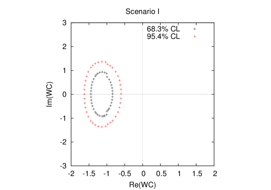
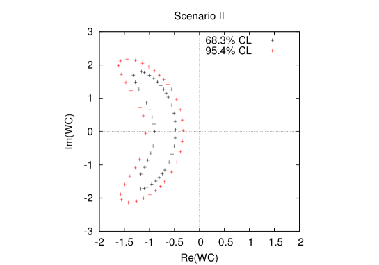
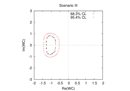
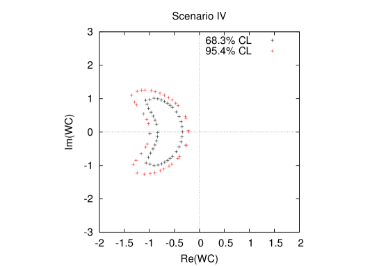
Figure 1: Allowed regions in the Re(WC)-Im(WC) plane for the four model-independent scenarios I-IV. See Table 1 for definitions of Re(WC) and Im(WC) in each of the four scenarios.

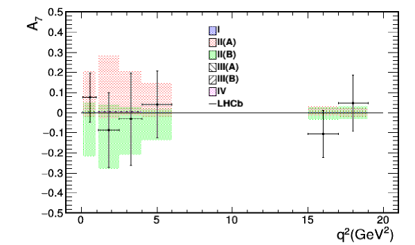
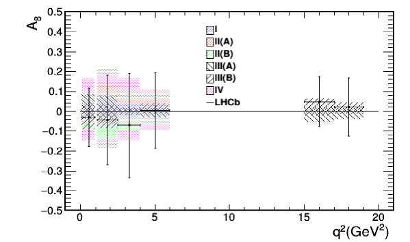
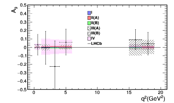
Figure 2: Predictions of the CP asymmetries $A_{7}$, $A_{8}$ and $A_{9}$ at the $2\sigma$ level for the four model-independent scenarios I-IV.

This then confirms the hypothesis that CP-violating observables can potentially be used to distinguish the various NP models proposed to explain the $b\to s\mu^{+}\mu^{-}$ anomalies. This said, one must be careful not to read too much into the model-independent results. If NP is present in $b\to s\mu^{+}\mu^{-}$ decays, it is due to a specific model. And this model may have other constraints, either theoretical or experimental, that may significantly change the predictions. That is, since the model-independent fits have the fewest constraints, the CP-violating effects shown in Fig. 2 are the largest possible. In a particular model, there may be additional constraints, which will reduce the predicted sizes of the CP asymmetries. For this reason, while a model-independent analysis is useful to get a general idea of what is possible, real predictions require a model-dependent analysis. We turn to this in the following sections.

IV Model-dependent Fits

Many models have been proposed to explain the $b\to s\mu^{+}\mu^{-}$ anomalies, of both the LQ CCO ; AGC ; HS1 ; GNR ; VH ; SM ; FK ; BFK ; BKSZ and $Z^{\prime}$ CCO ; Crivellin:2015lwa ; Isidori ; dark ; Chiang ; Virto ; GGH ; BG ; BFG ; Perimeter ; CDH ; SSV ; CHMNPR ; CMJS ; BDW ; FNZ ; AQSS ; CFL ; Hou ; CHV ; CFV ; CFGI ; IGG ; BdecaysDM ; Bhatia:2017tgo variety. Rather than considering each model individually, in this section we perform general analyses of the two types of models. The aim is to answer two questions. First, what are the properties of models required in order to provide good fits to the $b\to s\mu^{+}\mu^{-}$ data? Second, which of these good-fit models can also generate sizeable CP-violating asymmetries in $B\to K^{(*)}\mu^{+}\mu^{-}$? We separately examine LQ and $Z^{\prime}$ models.

IV.1 Leptoquarks

The list of all possible LQ models that couple to SM particles through dimension $\leq 4$ operators can be found in Ref. AGC . There are five spin-0 and five spin-1 LQs, denoted $\Delta$ and $V$ respectively, with couplings

$${\cal L}_{\Delta} = (y_{\ell u}{\bar{\ell}}_{L}u_{R}+y_{eq}\,{\bar{e}}_{R}i\tau_{2}q_{L})\Delta_{-7/6}+y_{\ell d}\,{\bar{\ell}}_{L}d_{R}\Delta_{-1/6}+(y_{\ell q}\,{\bar{\ell}}^{c}_{L}i\tau_{2}q_{L}+y_{eu}\,{\bar{e}}^{c}_{R}u_{R})\Delta_{1/3}$$

$$+~{}y_{ed}\,{\bar{e}}^{c}_{R}d_{R}\Delta_{4/3}+y^{\prime}_{\ell q}\,{\bar{\ell}}^{c}_{L}i\tau_{2}{\vec{\tau}}q_{L}\cdot{\vec{\Delta}}^{\prime}_{1/3}+h.c.$$

$${\cal L}_{V} = (g_{\ell q}\,{\bar{\ell}}_{L}\gamma_{\mu}q_{L}+g_{ed}\,{\bar{e}}_{R}\gamma_{\mu}d_{R})V^{\mu}_{-2/3}+g_{eu}\,{\bar{e}}_{R}\gamma_{\mu}u_{R}V^{\mu}_{-5/3}+g^{\prime}_{\ell q}\,{\bar{\ell}}_{L}\gamma_{\mu}{\vec{\tau}}q_{L}\cdot{\vec{V}}^{\prime\mu}_{-2/3}$$ (7)

$$+~{}(g_{\ell d}\,{\bar{\ell}}_{L}\gamma_{\mu}d_{R}^{c}+g_{eq}\,{\bar{e}}_{R}\gamma_{\mu}q^{c}_{L})V^{\mu}_{-5/6}++g_{\ell u}\,{\bar{\ell}}_{L}\gamma_{\mu}u_{R}^{c}V^{\mu}_{1/6}+h.c.$$

In the fermion currents and in the subscripts of the couplings, $q$ and $\ell$ represent left-handed quark and lepton $SU(2)_{L}$ doublets, respectively, while $u$, $d$ and $e$ represent right-handed up-type quark, down-type quark and charged lepton $SU(2)_{L}$ singlets, respectively. The LQs transform as follows under $SU(3)_{c}\times SU(2)_{L}\times U(1)_{Y}$:

$$\Delta_{-7/6}:({\bar{3}},2,-7/6)~{}~{},~{}~{}~{}~{}\Delta_{-1/6}:({\bar{3}},2,-1/6)~{}~{},~{}~{}~{}~{}\Delta_{1/3}:({\bar{3}},1,1/3)~{},$$

$$\Delta_{4/3}:({\bar{3}},1,4/3)~{}~{},~{}~{}~{}~{}{\vec{\Delta}}^{\prime}_{1/3}:({\bar{3}},3,1/3)~{},$$

$$V^{\mu}_{-2/3}:({\bar{3}},1,-2/3)~{}~{},~{}~{}~{}~{}V^{\mu}_{-5/3}:({\bar{3}},1,-5/3)~{}~{},~{}~{}~{}~{}{\vec{V}}^{\prime\mu}_{-2/3}:({\bar{3}},3,-2/3)~{},$$

$$V^{\mu}_{-5/6}:({\bar{3}},2,-5/6)~{}~{},~{}~{}~{}~{}V^{\mu}_{1/6}:({\bar{3}},2,-5/3)~{}.$$ (8)

Note that here the hypercharge is defined as $Y=Q_{em}-I_{3}$.

In Eq. (7), the LQs can couple to fermions of any generation. To specify which particular fermions are involved, we add superscripts to the couplings. For example, $g^{\prime\mu s}_{\ell q}$ is the coupling of the ${\vec{V}}^{\prime\mu}_{-2/3}$ LQ to a left-handed $\mu$ (or $\nu_{\mu}$) and a left-handed $s$. Similarly, $y_{eq}^{\mu b}$ is the coupling of the $\Delta_{-7/6}$ LQ to a right-handed $\mu$ and a left-handed $b$. These couplings are relevant for $b\to s\mu^{+}\mu^{-}$ (and possibly $b\to s\nu{\bar{\nu}}$). Note that the $V^{\mu}_{-5/3}$ and $V^{\mu}_{1/6}$ LQs do not contribute to $b\to s\ell^{+}\ell^{-}$.

A number of these LQs, and their effects on $b\to s\mu^{+}\mu^{-}$ and other decays, have been analyzed separately. For example, in Ref. Sakakietal , it was pointed out that four LQs can contribute to ${\bar{B}}\to D^{(*)+}\tau^{-}{\bar{\nu}}_{\tau}$. They are: a scalar isosinglet with $Y=1/3$, a scalar isotriplet with $Y=1/3$, a vector isosinglet with $Y=-2/3$, and a vector isotriplet with $Y=-2/3$. These are respectively $\Delta_{1/3}$, ${\vec{\Delta}}^{\prime}_{1/3}$, $V^{\mu}_{-2/3}$ and ${\vec{V}}^{\prime\mu}_{-2/3}$. In Ref. Sakakietal , they are called $S_{1}$, $S_{3}$, $U_{1}$ and $U_{3}$, respectively, and we adopt this nomenclature below.

The $S_{3}$ LQ has been studied in the context of $b\to s\mu^{+}\mu^{-}$ in Refs. HS1 ; GNR ; VH ; SM . $U_{1}$ has been examined in Refs. CCO ; RKRDmodels . In Ref. FK , the $U_{3}$ LQ was proposed as an explanation of the $b\to s\mu^{+}\mu^{-}$ anomalies. Finally, in Refs. BFK ; BKSZ it was claimed that the tree-level exchange of a $\Delta_{-1/6}$ LQ can account for the $b\to s\mu^{+}\mu^{-}$ results.

There are therefore quite a few LQ models that contribute to $b\to s\mu^{+}\mu^{-}$, several of which have been proposed as explanations of the $B$-decay anomalies. We would like to have a definitive answer to the following question: which of the LQs in Eq. (7) can actually explain the $b\to s\mu^{+}\mu^{-}$ anomalies? Rather than rely on previous work, we perform an independent analysis ourselves.

IV.1.1 LQ fits

The difference between model-independent and model-dependent fits is that, within a particular model, there may be contributions to new observables and/or new operators, and this must be taken into account in the fit. In the case of LQ models, the LQs contribute to a variety of operators. In addition to $O^{(\prime)}_{9,10}$ [Eq. (2)], there may be contributions to

$$O^{(\prime)}_{\nu}=[{\bar{s}}\gamma_{\mu}P_{L(R)}b][{\bar{\nu}}_{\mu}\gamma^{\mu}(1-\gamma_{5})\nu_{\mu}]~{},$$ (9)

$$O^{(\prime)}_{S}=[{\bar{s}}P_{R(L)}b][{\bar{\mu}}\mu]~{}~{},~{}~{}~{}~{}O^{(\prime)}_{P}=[{\bar{s}}P_{R(L)}b][{\bar{\mu}}\gamma_{5}\mu] ~{}.$$

$O^{(\prime)}_{\nu}$ contributes to $b\to s\nu_{\mu}{\bar{\nu}}_{\mu}$, while $O^{(\prime)}_{S}$ and $O^{(\prime)}_{P}$ are additional contributions to $b\to s\mu^{+}\mu^{-}$. Based on the couplings in Eq. (7), it is straightforward to work out which Wilson coefficients are affected by each LQ. These are shown in Table 2 AGC . Although the scalar LQs do not contribute to $O^{(\prime)}_{S,P}$, some vector LQs do. For these we have $C_{P}^{\mu\mu}({\rm NP})=-C_{S}^{\mu\mu}({\rm NP})$ and $C_{P}^{\prime\mu\mu}({\rm NP})=C_{S}^{\prime\mu\mu}({\rm NP})$.

LQ	$C_{9}^{\mu\mu}({\rm NP})$	$C_{10}^{\mu\mu}({\rm NP})$	$C_{9}^{\prime\mu\mu}({\rm NP})$	$C_{10}^{\prime\mu\mu}({\rm NP})$
	$C_{S}^{\mu\mu}({\rm NP})$	$C_{S}^{\prime\mu\mu}({\rm NP})$	$C_{\nu}^{\mu\mu}({\rm NP})$	$C_{\nu}^{\prime\mu\mu}({\rm NP})$
$\Delta_{1/3}~{}[S_{1}]$	0	0	0	0
	0	0	$\frac{1}{2}y_{\ell q}^{\mu b}(y_{\ell q}^{\mu s})^{*}$	0
${\vec{\Delta}}^{\prime}_{1/3}~{}[S_{3}]$	$y_{\ell q}^{\prime\mu b}(y_{\ell q}^{\prime\mu s})^{*}$	$-y_{\ell q}^{\prime\mu b}(y_{\ell q}^{\prime\mu s})^{*}$	0	0
	0	0	$\frac{1}{2}y_{\ell q}^{\prime\mu b}(y_{\ell q}^{\prime\mu s})^{*}$	0
$\Delta_{-7/6}$	$-\frac{1}{2}y_{eq}^{\mu b}(y_{eq}^{\mu s})^{*}$	$-\frac{1}{2}y_{eq}^{\mu b}(y_{eq}^{\mu s})^{*}$	0	0
	0	0	0	0
$\Delta_{-1/6}$	0	0	$-\frac{1}{2}y_{\ell d}^{\mu b}(y_{\ell d}^{\mu s})^{*}$	$\frac{1}{2}y_{\ell d}^{\mu b}(y_{\ell d}^{\mu s})^{*}$
	0	0	0	$-\frac{1}{2}y_{\ell d}^{\mu b}(y_{\ell d}^{\mu s})^{*}$
$\Delta_{4/3}$	0	0	$\frac{1}{2}y_{ed}^{\mu b}(y_{ed}^{\mu s})^{*}$	$\frac{1}{2}y_{ed}^{\mu b}(y_{ed}^{\mu s})^{*}$
	0	0	0	0
$V^{\mu}_{-2/3}~{}[U_{1}]$	$-g_{\ell q}^{\mu b}(g_{\ell q}^{\mu s})^{*}$	$g_{\ell q}^{\mu b}(g_{\ell q}^{\mu s})^{*}$	$-g_{ed}^{\mu b}(g_{ed}^{\mu s})^{*}$	$-g_{ed}^{\mu b}(g_{ed}^{\mu s})^{*}$
	$2g_{\ell q}^{\mu b}(g_{ed}^{\mu s})^{*}$	$2(g_{\ell q}^{\mu s})^{*}g_{ed}^{\mu b}$	0	0
${\vec{V}}^{\prime\mu}_{-2/3}~{}[U_{3}]$	$-g_{\ell q}^{\prime\mu b}(g_{\ell q}^{\prime\mu s})^{*}$	$g_{\ell q}^{\prime\mu b}(g_{\ell q}^{\prime\mu s})^{*}$	0	0
	0	0	$-2g_{\ell q}^{\prime\mu b}(g_{\ell q}^{\prime\mu s})^{*}$	0
$V^{\mu}_{-5/6}$	$g_{eq}^{\mu s}(g_{eq}^{\mu b})^{*}$	$g_{eq}^{\mu s}(g_{eq}^{\mu b})^{*}$	$g_{\ell d}^{\mu s}(g_{\ell d}^{\mu b})^{*}$	$-g_{\ell d}^{\mu s}(g_{\ell d}^{\mu b})^{*}$
	$2g_{\ell d}^{\mu s}(g_{eq}^{\mu b})^{*}$	$2(g_{\ell d}^{\mu b})^{*}g_{eq}^{\mu s}$	0	$g_{\ell d}^{\mu s}(g_{\ell d}^{\mu b})^{*}$

Table 2: Contributions of the different LQs to the Wilson coefficients of various operators. The normalization $K\equiv\pi/(\sqrt{2}\alpha G_{F}V_{tb}V_{ts}^{*}M_{LQ}^{2})$ has been factored out. For $M_{LQ}=1$ TeV, $K=-644.4$.

There are several observations one can make from this Table. First, not all of the LQs contribute to $b\to s\mu^{+}\mu^{-}$: $\Delta_{1/3}$ contributes only to $b\to s\nu{\bar{\nu}}$. Second, $U_{1}$ has two couplings, $g_{\ell q}$ and $g_{ed}$. If both are allowed simultaneously, scalar operators are generated, and these can also contribute to $b\to s\mu^{+}\mu^{-}$. This must be taken into account in the model-dependent fits. The situation is similar for $V^{\mu}_{-5/6}$. Finally, the $S_{3}$ and $U_{3}$ LQs both have $C_{9}^{\mu\mu}({\rm NP})=-C_{10}^{\mu\mu}({\rm NP})$; they are differentiated only by their contributions to $C_{\nu}^{\mu\mu}({\rm NP})$.

At this stage, we can perform model-dependent fits to determine which of the LQ models can explain the data. First of all, the SM alone does not provide a good fit. We find, for 106 degrees of freedom, that

$$\chi^{2}_{SM}/d.o.f.\ =1.34~{}~{},~{}~{}~{}~{}{\hbox{p-value $=0.01$.}}$$ (10)

We therefore confirm that the $b\to s\mu^{+}\mu^{-}$ anomalies suggest the presence of NP.

For the scalar LQs, the results of the fits using only the $b\to s\mu^{+}\mu^{-}$ data are shown in Table 3 (we address the $b\to s\nu{\bar{\nu}}$ data below). For the $S_{3}$ LQ, there are two best-fit solutions, labeled (A) and (B). (The two solutions have the same best-fit values for Re(coupling), but opposite signs for the best-fit values of Im(coupling).) From this Table, we see that only the $S_{3}$ LQ provides an acceptable fit to the data. Despite the claims of Refs. BFK ; BKSZ , the $\Delta_{-1/6}$ LQ does not explain the $b\to s\mu^{+}\mu^{-}$ anomalies.

LQ	Coupling	[Re(coupling), Im(coupling)] $\times 10^{3}$	pull
${\vec{\Delta}}^{\prime}_{1/3}~{}[S_{3}]$	$y_{\ell q}^{\prime\mu b}(y_{\ell q}^{\prime\mu s})^{*}$	(A)   [$(1.5\pm 0.5)$, $(-1.9\pm 1.2)$ ]	4.2
		(B)   [$(1.4\pm 0.5)$, $(1.7\pm 1.3)$ ]	4.0
$\Delta_{-7/6}$	$y_{eq}^{\mu b}(y_{eq}^{\mu s})^{*}$	[$(0.1\pm 0.7)$, $(0.0\pm 1.3)$ ]	0.1
$\Delta_{-1/6}$	$y_{\ell d}^{\mu b}(y_{\ell d}^{\mu s})^{*}$	[$(-0.1\pm 0.3)$, $(-0.1\pm 1.3)$ ]	0.4
$\Delta_{4/3}$	$y_{ed}^{\mu b}(y_{ed}^{\mu s})^{*}$	[$(0.2\pm 0.7)$, $(0.0\pm 0.9)$ ]	0.2

Table 3: Scalar LQs: best-fit values of the real and imaginary parts of the couplings, and the pull=$\sqrt{\chi^{2}_{SM}-\chi^{2}_{min}}$ of the fits, for $M_{LQ}=1$ TeV.

The vector LQs are more complicated because the $U_{1}$ and $V^{\mu}_{-5/6}$ LQs each have two couplings. The $U_{1}$ case, where the two couplings are $g_{\ell q}$ and $g_{ed}$, is particularly interesting. If $g_{ed}^{ij}=0$, we have $C_{9}^{\mu\mu}({\rm NP})=-C_{10}^{\mu\mu}({\rm NP})$, like the $S_{3}$ and $U_{3}$ LQs. (Recall that we found that $S_{3}$ can explain the $b\to s\mu^{+}\mu^{-}$ anomalies.) And if $g_{ed}^{\mu b}(g_{ed}^{\mu s})^{*}=-g_{\ell q}^{\mu b}(g_{\ell q}^{\mu s})^{*}$, we have $C_{9}^{\mu\mu}({\rm NP})=-C_{10}^{\mu\mu}({\rm NP})=-C_{9}^{\prime\mu\mu}({\rm NP})=-C_{10}^{\prime\mu\mu}({\rm NP})$, which is scenario IV of Eq. (6), and is also found to explain the anomalies. To explore the $U_{1}$ model fully, we perform three fits. Fit (1) has $g_{ed}^{ij}=0$, fit (2) has $g_{ed}^{\mu b}=g_{\ell q}^{\mu b}$ and $g_{ed}^{\mu s}=-g_{\ell q}^{\mu s}$ (which gives $g_{ed}^{\mu b}(g_{ed}^{\mu s})^{*}=-g_{\ell q}^{\mu b}(g_{\ell q}^{\mu s})^{*}$), and fit (3) allows the $g_{ed}^{ij}$ to be free. For the $V^{\mu}_{-5/6}$ LQ, here too we can allow all couplings to vary, but for simplicity we set $g_{ld}^{ij}=0$. However, we have checked that, even if we vary all the couplings, this model does not provide a good fit.

Regarding fit (3), a few comments are useful. Although we allow all couplings to vary, the constraints apply only to products of couplings. This allows some freedom: the magnitude of $g_{\ell q}^{\mu s}$ does not affect the best-fit values of the WCs, so we simply set it to 1. Also, in order to avoid problems with correlations in the fits, we set $g_{\ell q}^{\mu s}$ and $g_{ed}^{\mu s}$ to fixed real values. Finally, in Ref. BK*mumulatestfit1 it was found that the global fit requires $C_{S}^{\mu\mu}({\rm NP})\ll C_{9}^{\mu\mu}({\rm NP})$, i.e., $g_{ed}^{\mu s}/g_{\ell q}^{\mu s}\ll 1$. We have found that $g_{ed}^{\mu s}/g_{\ell q}^{\mu s}\simeq 0.02$ leads to a fit with a pull of around 4.

LQ	Couplings	[Re(coupling), Im(coupling)] $\times 10^{3}$	pull
$V^{\mu}_{-2/3}~{}[U_{1}]$:
(1)	$g_{\ell q}^{\mu b}(g_{\ell q}^{\mu s})^{*}$	(A)  [$(-1.5\pm 0.5)$, $(1.9\pm 1.2)$ ]	4.2
		(B)   [$(-1.4\pm 0.5)$, $(-1.7\pm 1.3)$ ]	4.0
(2)	$g_{\ell q}^{\mu b}(g_{\ell q}^{\mu s})^{*}$	[$(-0.01\pm 0.02)$, $(0.0\pm 0.02)$ ]	0.5
(3)	$g_{\ell q}^{\mu b}$	(A)    [$(-1.2\pm 0.4)$, $(1.7\pm 1.1)$ ]
	$g_{ed}^{\mu b}$	[$(0.07\pm 0.04)$, $(0.02\pm 0.08)$ ]	4.3
		(B)    [$(-1.3\pm 0.4)$, $(-1.9\pm 1.0)$ ]
		[$(0.06\pm 0.05)$, $(-0.02\pm 0.08)$ ]	4.3
${\vec{V}}^{\prime\mu}_{-2/3}~{}[U_{3}]$	$g_{\ell q}^{\prime\mu b}(g_{\ell q}^{\prime\mu s})^{*}$	(A)   [$(-1.5\pm 0.5)$, $(1.9\pm 1.2)$ ]	4.2
		(B)   [$(-1.4\pm 0.5)$, $(-1.7\pm 1.3)$ ]	4.0
$V^{\mu}_{-5/6}$	$g_{eq}^{\mu s}(g_{eq}^{\mu b})^{*}$	[$(0.0\pm 0.4)$, $(0.0\pm 1.2)$ ]	0.0

Table 4: Vector LQs: best-fit values of the real and imaginary parts of the couplings, and the pull=$\sqrt{\chi^{2}_{SM}-\chi^{2}_{min}}$ of the fits, for $M_{LQ}=1$ TeV.

The results of the fits are shown in Table 4. There are several notable features:

1. We see that the $b\to s\mu^{+}\mu^{-}$ anomalies can be explained with the $U_{1}$ LQ [fit (1)] and the $U_{3}$ LQ. Like the $S_{3}$ LQ, they have $C_{9}^{\mu\mu}({\rm NP})=-C_{10}^{\mu\mu}({\rm NP})$. Indeed, because only $b\to s\mu^{+}\mu^{-}$ data were used in the fits, the fit results are identical for all three LQ models.

2. A good fit is also found with the $U_{1}$ LQ [fit (3)]. However, the best-fit solution has $g_{ed}^{\mu b}\simeq 0$, so that this is essentially the same as the $U_{1}$ LQ [fit (1)].

3. The $U_{1}$ LQ model [fit (2)] has been constructed to satisfy $C_{9}^{\mu\mu}({\rm NP})=-C_{10}^{\mu\mu}({\rm NP})=-C_{9}^{\prime\mu\mu}({\rm NP})=-C_{10}^{\prime\mu\mu}({\rm NP})$. Despite this, the model does not provide a good fit of the $b\to s\mu^{+}\mu^{-}$ data. The reason is that, in this model, there are also important contributions to the scalar operators of Eq. (9). However, the measurement of $B^{0}_{s}\to\mu^{+}\mu^{-}$ puts strong constraints on such contributions. The result is that one cannot explain the anomalies in $B\to K^{*}\mu^{+}\mu^{-}$, $B^{0}_{s}\to\phi\mu^{+}\mu^{-}$ and $R_{K}$, while simultaneously agreeing with the measurement of $B^{0}_{s}\to\mu^{+}\mu^{-}$. This provides an explicit example of how the “model-independent,” results of Eq. (6) do not necessarily apply to particular models.

4. The $V^{\mu}_{-5/6}$ LQ model does not provide a good fit of the $b\to s\mu^{+}\mu^{-}$ data.

We therefore see that, of all the scalar and vector LQ models, only $S_{3}$, $U_{1}$ and $U_{3}$ can explain the $b\to s\mu^{+}\mu^{-}$ anomalies. Furthermore, within the context of $b\to s\mu^{+}\mu^{-}$ processes, the models are equivalent, since they all have $C_{9}^{\mu\mu}({\rm NP})=-C_{10}^{\mu\mu}({\rm NP})$.

Finally, recall that the aim of this analysis is to differentiate different $b\to s\mu^{+}\mu^{-}$ NP models through measurements of CP-violating asymmetries in $B\to K^{(*)}\mu^{+}\mu^{-}$. As noted in the introduction, such CP asymmetries can be sizeable only if there is a significant NP weak phase. For the LQ model, we see from Table 4 that the real and imaginary parts of the coupling are of similar sizes. The NP weak phase is therefore not small, so that large CP asymmetries can be expected.

IV.1.2 $b\to s\nu{\bar{\nu}}$

Above, we have argued that the $S_{3}$, $U_{1}$ and $U_{3}$ LQ models are equivalent. However, from Table 2, note that the three LQs contribute differently to $C_{\nu}^{\mu\mu}({\rm NP})$, the WC associated with $O_{\nu}$, the operator responsible for $b\to s\nu_{\mu}{\bar{\nu}}_{\mu}$. To be specific, the $S_{3}$ and $U_{3}$ LQs have $C_{\nu}^{\mu\mu}({\rm NP})=\frac{1}{2}C_{9}^{\mu\mu}({\rm NP})$ and $C_{\nu}^{\mu\mu}({\rm NP})=2C_{9}^{\mu\mu}({\rm NP})$, respectively, while the $U_{1}$ LQ has $C_{\nu}^{\mu\mu}({\rm NP})=0$. This means that, for $S_{3}$ and $U_{3}$, constraints on $C_{\nu}^{\mu\mu}({\rm NP})$ translate into additional constraints on $C_{9}^{\mu\mu}({\rm NP})$. This then raises the question: could these three LQ solutions be distinguished by the $b\to s\nu{\bar{\nu}}$ data?

The effective Hamiltonian relevant for $b\to s\nu{\bar{\nu}}$ is Buras:2014fpa

$$H_{\rm eff}=-\frac{\alpha G_{F}}{\sqrt{2}\pi}V_{tb}V_{ts}^{*}\sum_{\ell}C_{L}^{\ell}(\bar{s}\gamma_{\mu}P_{L}b)(\bar{\nu}_{\ell}\gamma^{\mu}(1-\gamma_{5})\nu_{\ell})~{}.$$ (11)

The WC contains both the SM and NP contributions: $C_{L}^{\ell}=C_{L}^{\rm SM}+C_{\nu}^{\ell\ell}({\rm NP})$; it allows for NP that is lepton flavor non-universal. This is appropriate to the present case, as the LQs have only a nonzero $C_{\nu}^{\mu\mu}({\rm NP})$. The SM WC is

$$C_{L}^{\rm SM}=-X_{t}/s_{W}^{2}~{},$$ (12)

where $s_{W}\equiv\sin\theta_{W}$ and $X_{t}=1.469\pm 0.017$.

The latest $b\to s\nu{\bar{\nu}}$ measurements yield Grygier:2017tzo

$${\cal B}(B\rightarrow K\nu\bar{\nu}) < 1.6\times 10^{-5}~{},$$

$${\cal B}(B\rightarrow K^{*}\nu\bar{\nu}) < 2.7\times 10^{-5}~{}.$$ (13)

In Ref. Buras:2014fpa , the SM predictions for these decays were computed:

$${\cal B}(B\rightarrow K\nu\bar{\nu})|_{SM}=(3.98\pm 0.43\pm 0.19)\times 10^{-6}~{},$$

$${\cal B}(B\rightarrow K^{*}\nu\bar{\nu})|_{SM}=(9.19\pm 0.86\pm 0.50)\times 10^{-6}~{}.$$ (14)

We define

$${\cal R}_{K}\equiv\frac{{\cal B}(B\rightarrow K\nu\bar{\nu})}{{\cal B}_{SM}{(B\rightarrow K\nu\bar{\nu})}}~{}~{},~{}~{}~{}~{}{\cal R}_{K^{*}}\equiv\frac{{\cal B}(B\rightarrow K^{*}\nu\bar{\nu})}{{\cal B}_{SM}{(B\rightarrow K^{*}\nu\bar{\nu})}}~{}.$$ (15)

Using Eqs. (13) and (14), we obtain

$${\cal R}_{K}<4.0~{}~{},~{}~{}~{}~{}{\cal R}_{K^{*}}<2.9~{}.$$ (16)

From Ref. Buras:2014fpa , ${\cal R}_{K}$ and ${\cal R}_{K^{*}}$ can be written as

$${\cal R}_{K}={\cal R}_{K}^{*} = \frac{2}{3}+\frac{1}{3}\frac{|C_{L}^{SM}+C_{\nu}^{\mu\mu}({\rm NP})|^{2}}{|C_{L}^{SM}|^{2}}$$ (17)

$$= 1+\frac{2}{3}{\rm Re}(C_{\nu}^{\mu\mu}({\rm NP})/C_{L}^{SM})+\frac{1}{3}|C_{\nu}^{\mu\mu}({\rm NP})/C_{L}^{SM}|^{2}~{}.$$

Since $C_{\nu}^{\mu\mu}({\rm NP})$ is proportional to $C_{9}^{\mu\mu}({\rm NP})$, and since $|C_{9}^{\mu\mu}({\rm NP})|=O(1)$ (see Table 1, scenario II), the $b\to s\mu^{+}\mu^{-}$ data implies that $|C_{\nu}^{\mu\mu}({\rm NP})|$ is also $O(1)$. Can the $b\to s\nu{\bar{\nu}}$ data provide competitive constraints on $|C_{\nu}^{\mu\mu}({\rm NP})|$? Using the ${\cal R}_{K^{*}}$ bound of Eq. (16) (since it is stronger), and neglecting ${\rm Im}(C_{\nu}^{\mu\mu}({\rm NP}))$ in Eq. (17), we obtain

$$-10.1<{\rm Re}(C_{\nu}^{\mu\mu}({\rm NP}))<22.8~{}.$$ (18)

The above limit is significantly weaker than the result $|C_{\nu}^{\mu\mu}({\rm NP})|=O(1)$ coming from the fit to the $b\to s\mu^{+}\mu^{-}$ data. We therefore conclude that the $b\to s\nu{\bar{\nu}}$ data cannot be used to distinguish the $S_{3}$, $U_{1}$ and $U_{3}$ LQs.

Note that this conclusion may not hold if the LQs also couple to other leptons. For example, in Ref. RKRDmodels it was assumed that the LQs couple to $(\nu_{\tau},\tau^{-})_{L}$ in the gauge basis, and that couplings to $(\nu_{\mu},\mu^{-})_{L}$ are generated only when one transforms to the mass basis. In this case, the LQs contribute not only to $b\to s\nu_{\mu}{\bar{\nu}}_{\mu}$, but also to $b\to s\nu_{\tau}{\bar{\nu}}_{\tau}$, which can alter the above analysis. Indeed, in Ref. RKRDmodels it is found that constraints from $b\to s\nu{\bar{\nu}}$ are important in the comparison of the $S_{3}$, $U_{1}$ and $U_{3}$ LQs.

IV.2 $Z^{\prime}$ bosons

Perhaps the most obvious candidate for a NP contribution to $b\to s\mu^{+}\mu^{-}$ is the tree-level exchange of a $Z^{\prime}$ boson with a flavor-changing coupling ${\bar{s}}\gamma^{\mu}P_{L}bZ^{\prime}_{\mu}$. Given that it couples to two left-handed doublets, the $Z^{\prime}$ must transform as a singlet or triplet of $SU(2)_{L}$. The triplet option has been examined in Refs. CCO ; Crivellin:2015lwa ; Isidori ; dark ; Chiang ; Virto . (In this case, there is also a $W^{\prime}$ that can contribute to ${\bar{B}}\to D^{(*)+}\tau^{-}{\bar{\nu}}_{\tau}$ RKRD , another decay whose measurement exhibits a discrepancy with the SM RD_BaBar ; RD_Belle ; RD_LHCb .) If the $Z^{\prime}$ is a singlet of $SU(2)_{L}$, it must be the gauge boson associated with an extra $U(1)^{\prime}$. Numerous models of this type have been proposed, see Refs. GGH ; BG ; BFG ; Perimeter ; CDH ; SSV ; CHMNPR ; CMJS ; BDW ; FNZ ; AQSS ; CFL ; Hou ; CHV ; CFV ; CFGI ; IGG ; BdecaysDM ; Bhatia:2017tgo .

The vast majority of these $Z^{\prime}$ models use scenario II of Eq. (6): $C_{9}^{\mu\mu}({\rm NP})=-C_{10}^{\mu\mu}({\rm NP})$. Thus, although the underlying details of these models are different, in all cases we can write

$$\Delta{\cal L}_{Z^{\prime}} = J^{\mu}Z^{\prime}_{\mu}~{},$$

$${\rm where}\qquad J^{\mu} = g_{L}^{\mu\mu}\,\bar{L}\gamma^{\mu}P_{L}L+g_{L}^{bs}\,{\bar{\psi}}_{q2}\gamma^{\mu}P_{L}\psi_{q3}+h.c.$$ (19)

Here $\psi_{qi}$ is the quark doublet of the $i^{th}$ generation, and $L=(\nu_{\mu},\mu)^{T}$. When the heavy $Z^{\prime}$ is integrated out, we obtain the following effective Lagrangian containing 4-fermion operators:

$${\cal L}_{Z^{\prime}}^{eff}=-\frac{1}{2M_{Z^{\prime}}^{2}}J_{\mu}J^{\mu} \supset -\frac{g_{L}^{bs}g_{L}^{\mu\mu}}{M_{Z^{\prime}}^{2}}(\bar{s}\gamma^{\mu}P_{L}b)(\bar{\mu}\gamma^{\mu}P_{L}\mu)-\frac{(g_{L}^{bs})^{2}}{2M_{Z^{\prime}}^{2}}(\bar{s}\gamma^{\mu}P_{L}b)(\bar{s}\gamma^{\mu}P_{L}b)$$ (20)

$$\hskip 14.22636pt-~{}\frac{(g_{L}^{\mu\mu})^{2}}{M_{Z^{\prime}}^{2}}(\bar{\mu}\gamma^{\mu}P_{L}\mu)({\bar{\nu}}_{\mu}\gamma^{\mu}P_{L}\nu_{\mu})~{}.$$

The first 4-fermion operator is relevant for $b\to s\mu^{+}\mu^{-}$ transitions, the second operator contributes to $B^{0}_{s}$-${\bar{B}}^{0}_{s}$ mixing, and the third operator contributes to neutrino trident production.

Note that $g_{L}^{\mu\mu}$ must be real, since the leptonic current of Eq. (19) is self-conjugate. However, $g_{L}^{bs}$ can be complex, i.e., it can contain a weak phase. This phase can potentially lead to CP-violating effects in $B\to K^{(*)}\mu^{+}\mu^{-}$ via the first 4-fermion operators of Eq. (20). The question is: how large can this NP weak phase be? This is the question that is addressed in this subsection by considering constraints from $b\to s\mu^{+}\mu^{-}$, $B^{0}_{s}$-${\bar{B}}^{0}_{s}$ mixing, and neutrino trident production.

For $b\to s\mu^{+}\mu^{-}$ we have

$$C_{9}^{\mu\mu}({\rm NP})=-C_{10}^{\mu\mu}({\rm NP})=-\left[\frac{\pi}{\sqrt{2}G_{F}\alpha V_{tb}V_{ts}^{*}}\right]\,\frac{g_{L}^{bs}g_{L}^{\mu\mu}}{M_{Z^{\prime}}^{2}}~{}.$$ (21)

Turning to $B^{0}_{s}$-${\bar{B}}^{0}_{s}$ mixing, the SM contribution arises due to a box diagram, and is given by

$$NC_{VLL}^{\rm SM}\,({\bar{s}}_{L}\gamma^{\mu}b_{L})\,({\bar{s}}_{L}\gamma_{\mu}b_{L})~{},$$ (22)

where

$$N=\frac{G_{F}^{2}m_{W}^{2}}{16\pi^{2}}(V_{tb}V_{ts}^{*})^{2}~{},~{}~{}C_{VLL}^{\rm SM}=\eta_{B_{s}}x_{t}\left[1+\frac{9}{1-x_{t}}-\frac{6}{(1-x_{t})^{2}}-\frac{6x_{t}^{2}\ln x_{t}}{(1-x_{t})^{3}}\right]~{}.$$ (23)

Here $x_{t}\equiv m_{t}^{2}/m_{W}^{2}$ and $\eta_{B_{s}}=0.551$ is the QCD correction Buchalla:1995vs . Combining the SM and NP contributions, we define

$$NC_{VLL}\equiv|NC_{VLL}^{\rm SM}|e^{-2i\beta_{s}}+\frac{(g_{L}^{bs})^{2}}{2M_{Z^{\prime}}^{2}}~{},$$ (24)

where $-\beta_{s}={\rm arg}(V_{tb}V_{ts}^{*})$. This leads to

$$\Delta M_{s}=\frac{2}{3}m_{B_{s}}f_{B_{s}}^{2}\hat{B}_{B_{s}}\left|NC_{VLL}\right|~{}.$$ (25)

In addition, the weak phase of $B^{0}_{s}$-${\bar{B}}^{0}_{s}$ mixing is given by

$$\varphi_{s}={\rm arg}(NC_{VLL}).$$ (26)

From the above expressions, we see that, the larger $g_{L}^{bs}$ is, the more $Z^{\prime}$ models contribute to – and receive constraints from – $B^{0}_{s}$-${\bar{B}}^{0}_{s}$ mixing. The experimental measurements of the mixing parameters yield HFAG

$$\Delta M_{s}^{\rm exp} = 17.757\pm 0.021~{}{\rm ps}^{-1}~{},$$

$$\varphi_{s}^{c{\bar{c}}s} = -0.030\pm 0.033~{}.$$ (27)

These are to be compared with the SM predictions:

$$\Delta M_{s}^{\rm SM} = \frac{2}{3}m_{B_{s}}f_{B_{s}}^{2}\hat{B}_{B_{s}}|NC_{VLL}^{\rm SM}|=(17.9\pm 2.4)~{}{\rm ps}^{-1}~{},$$

$$\varphi_{s}^{c{\bar{c}s,{\rm SM}}} = -2\beta_{s}=-0.03704\pm 0.00064~{}.$$ (28)

In the above, for $\Delta M_{s}^{\rm SM}$, we have followed the computation of Ref. RKRDmodels , using $f_{B_{s}}\sqrt{\hat{B}_{B_{s}}}=270\pm 16$ MeV Aoki:2014nga ; Gamiz:2009ku ; Aoki:2016frl , $|V_{tb}V^{*}_{ts}|=0.0405\pm 0.0012$ pdg , and $\overline{m_{t}}=160$ GeV; $\varphi_{s}^{c{\bar{c}}s,{\rm SM}}$ is taken from Refs. Charles:2004jd ; Hocker:2001xe .

The $Z^{\prime}$ will also contribute to the production of $\mu^{+}\mu^{-}$ pairs in neutrino-nucleus scattering, $\nu_{\mu}N\to\nu_{\mu}N\mu^{+}\mu^{-}$ (neutrino trident production). At leading order, this process is effectively $\nu_{\mu}\gamma\to\nu_{\mu}\mu^{+}\mu^{-}$, and is produced by single-$W$/$Z$ exchange in the SM. This arises from the four-fermion effective operator

$$\mathcal{L}_{\text{eff:trident}}=\left[\bar{\mu}\gamma^{\mu}\left(C_{V}-C_{A}\gamma^{5}\right)\mu\right]\left[\bar{\nu}\gamma_{\mu}(1-\gamma^{5})\nu\right]\,,$$ (29)

with an external photon coupling to $\mu^{+}$ or $\mu^{-}$. In the SM, combining both $W$- and $Z$-exchange diagrams, we have Koike:1971tu ; Koike:1971vg ; Belusevic:1987cw ; Brown:1973ih

$$C_{V}^{\text{SM}}=-{g^{2}\over 8m_{W}^{2}}\left({1\over 2}+2s_{W}^{2}\right)~{}~{},~{}~{}~{}~{}C_{A}^{\text{SM}}=-{g^{2}\over 8m_{W}^{2}}\,{1\over 2}~{}.$$ (30)

On the other hand, the $Z^{\prime}$ boson contributes to Eq. (29) with the pure $V-A$ form:

$$C_{V}^{\rm NP}=C_{A}^{\rm NP}=-{(g_{L}^{\mu\mu})^{2}\over 4M_{Z^{\prime}}^{2}}\,.$$ (31)

The theoretical prediction is then

$$\left.{\sigma_{\text{SM+NP}}\over\sigma_{\text{SM}}}\right|_{\nu N\to\nu N\mu^{+}\mu^{-}} = {(C_{V}^{\text{SM}}+C_{V}^{\text{NP}})^{2}+(C_{A}^{\text{SM}}+C_{A}^{\text{NP}})^{2}\over(C_{V}^{\text{SM}})^{2}+(C_{A}^{\text{SM}})^{2}}$$

$$= \frac{1}{1+(1+4s_{W}^{2})^{2}}\left[\left(1+\frac{v^{2}(g_{L}^{\mu\mu})^{2}}{M_{{Z}^{{}^{\prime}}}^{2}}\right)^{2}+\left(1+4s_{W}^{2}+\frac{v^{2}(g_{L}^{\mu\mu})^{2}}{M_{{Z}^{{}^{\prime}}}^{2}}\right)^{2}\right]~{},$$

to be compared with the experimental measurement CCFR :

$$\left.{\sigma_{\text{exp.}}\over\sigma_{\text{SM}}}\right|_{\nu N\to\nu N\mu^{+}\mu^{-}}=0.82\pm 0.28~{}.$$ (33)

The net effect is that this will provide an upper limit on $(g_{L}^{\mu\mu})^{2}/M_{Z^{\prime}}^{2}$. For $M_{Z^{\prime}}=1$TeV and $v=246$ GeV, we obtain the following $1\sigma$ bound on the coupling:

$$|g_{L}^{\mu\mu}|\leq 1.25~{}.$$ (34)

We now perform a fit within the context of this $Z^{\prime}$ model. The fit includes the measurements of the $b\to s\mu^{+}\mu^{-}$ observables, $B^{0}_{s}$-${\bar{B}}^{0}_{s}$ mixing (magnitude and phase), and the cross section for neutrino trident production. There are 107 degrees of freedom.

$g_{L}^{\mu\mu}$	[Re($g_{L}^{bs}$),Im($g_{L}^{bs}$)]$\times 10^{3}$	pull
0.01	[$(-2.4\pm 2.1)$, $(-0.1\pm 0.7)$ ]	0.8
0.05	[$(-3.9\pm 1.2)$, $(0.0\pm 0.5)$ ]	2.3
0.1	[$(-4.3\pm 1.0)$, $(0.0\pm 0.4)$ ]	3.3
0.2	[$(-3.9\pm 0.8)$, $(0.0\pm 0.5)$ ]	4.0
0.4	[$(-2.1\pm 0.5)$, $(-0.1\pm 0.8)$ ]	4.2
0.5	[$(-1.8\pm 0.5)$, $(-0.1\pm 0.9)$ ]	4.0
0.8	[$(-1.1\pm 0.3)$, $(-0.1\pm 1.5)$ ]	4.0
1.0	[$(-0.8\pm 0.3)$, $(-0.4\pm 3.1)$ ]	4.0

Table 5: $Z^{\prime}$ model: best-fit values of the real and imaginary parts of $g_{L}^{bs}$, and the pull=$\sqrt{\chi^{2}_{SM}-\chi^{2}_{min}}$ of the fits, for various values of $g_{L}^{\mu\mu}$ and $M_{Z^{\prime}}=1$ TeV.

Our results are summarized in Table 5. We see that a good fit is obtained for $g_{L}^{\mu\mu}\geq 0.1$. (Smaller values of $g_{L}^{\mu\mu}$ imply larger values for $g_{L}^{bs}$, which are disfavored by measurements of $B^{0}_{s}$-${\bar{B}}^{0}_{s}$ mixing.)

Once again, recall that the ultimate aim of this study is to compare the predictions of different models for the CP-violating asymmetries in $B\to K^{(*)}\mu^{+}\mu^{-}$. Such asymmetries can be sizeable only if the NP weak phase is large. However, from Table 5, we see that Im($g_{L}^{bs}$)/Re($g_{L}^{bs}$) is O(1) only for $g_{L}^{\mu\mu}=0.8$, 1.0. It is intermediate for $g_{L}^{\mu\mu}=0.4$, 0.5, and is small for $g_{L}^{\mu\mu}=0.1$, 0.2. We therefore expect that models with different values of $g_{L}^{\mu\mu}$ will predict different values of the CP asymmetries, potentially allowing them to be differentiated.

From the above, we see that a large NP weak phase can only be produced in $Z^{\prime}$ models if $g_{L}^{\mu\mu}$ is large. However, note that, while this is a necessary condition, it is not sufficient. In a particular $Z^{\prime}$ model, it is necessary to have a mechanism whereby $g_{L}^{bs}$ can have a weak phase. This is not the case for all models. As an example, in some models, the $Z^{\prime}$ couples only to ${\bar{b}}b$ in the gauge basis. Its coupling constant is therefore real. The flavor-changing coupling to ${\bar{s}}b$ is only generated when transforming to the mass basis. However, in Refs. CCO ; RKRDmodels , this transformation involves only the second and third generations. In other words, it is essentially a $2\times 2$ rotation, which is real. In these models a weak phase in $g_{L}^{bs}$ cannot be generated.

V CP Asymmetries: Model-dependent Predictions

In the previous section, we have identified the characteristics of NP models that can explain the $b\to s\mu^{+}\mu^{-}$ anomalies. We have found that there are three LQ models – $S_{3}$, $U_{1}$, $U_{3}$ – that can do this. All have $C_{9}^{\mu\mu}({\rm NP})=-C_{10}^{\mu\mu}({\rm NP})$ and so are equivalent, as far as $b\to s\mu^{+}\mu^{-}$ processes are concerned. There is a whole spectrum of $Z^{\prime}$ models that can explain the $b\to s\mu^{+}\mu^{-}$ data. What is required is that the $Z^{\prime}$ have couplings $g_{L}^{bs}\,{\bar{s}}\gamma^{\mu}P_{L}bZ^{\prime}_{\mu}$ and $g_{L}^{\mu\mu}\,{\bar{\mu}}\gamma^{\mu}P_{L}\mu Z^{\prime}_{\mu}$, and that $g_{L}^{\mu\mu}$ be $\geq 0.1$.

The purpose of this paper is to investigate whether these models can be distinguished by measurements of CP-violating asymmetries in $B\to K^{*}\mu^{+}\mu^{-}$ and $B\to K\mu^{+}\mu^{-}$. To this end, the next step is then to compute the predictions of all models for the allowed ranges of the various asymmetries. For the LQ and $Z^{\prime}$ models, the best-fit values and errors of the real and imaginary parts of the NP couplings are given in Tables 3 and 5, respectively. (For the LQ model, the allowed region in the Re(WC)-Im(WC) plane is shown in the upper right plot of Fig. 1 (scenario II).) With these we can calculate the predictions for the asymmetries for all models.

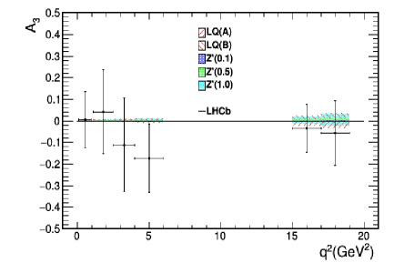
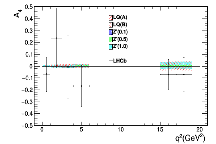
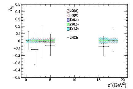
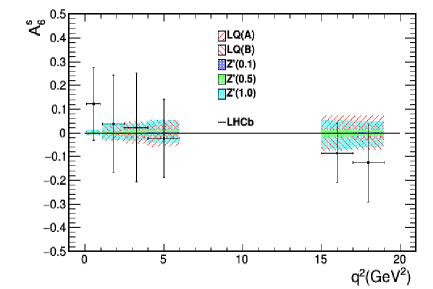
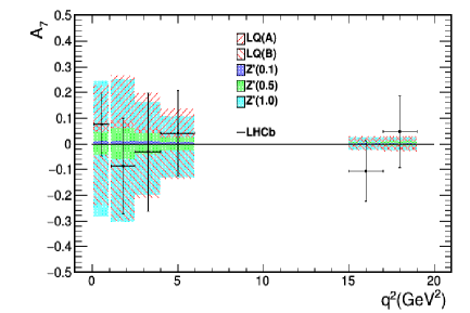
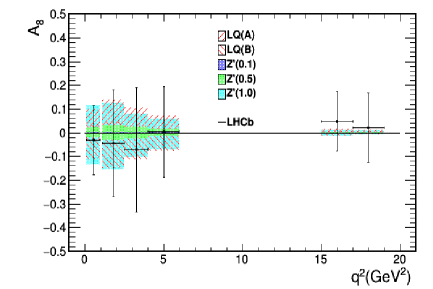
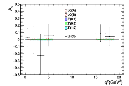
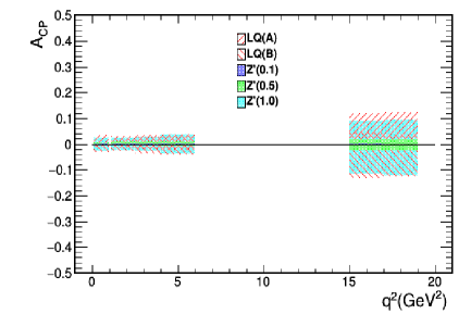
Figure 3: Predictions of the LQ model (solutions (A) and (B)) and the $Z^{\prime}$ model with $g_{L}^{\mu\mu}=0.1,0.5,1.0$ for the CP asymmetries $A_{3}$-$A_{9}$ in $B^{0}\to K^{*0}\mu^{+}\mu^{-}$ and $A_{\rm CP}$ in $B\to K\mu^{+}\mu^{-}$. In the models, the real and imaginary parts of the couplings are allowed to vary by $\pm 2\sigma$.

In Fig. 3, we present the predictions for the CP asymmetries $A_{3}$-$A_{9}$ in $B^{0}\to K^{*0}\mu^{+}\mu^{-}$ and $A_{\rm CP}$ in $B\to K\mu^{+}\mu^{-}$. We consider the LQ model (solutions (A) and (B)) and the $Z^{\prime}$ model with $g_{L}^{\mu\mu}=0.1,0.5,1.0$. The ranges of the asymmetries are obtained by allowing the real and imaginary parts of the couplings to vary by $\pm 2\sigma$ (taking correlations into account). From these figures we see that

• The predictions of the $Z^{\prime}$ model with $g_{L}^{\mu\mu}=1.0$ are very similar to those of the LQ model in which solutions (A) and (B) are added.

• Even in the presence of NP, the asymmetries $A_{3}$, $A_{4}$, $A_{5}$, and $A_{9}$ are very small and probably unmeasurable.

• In the LQ and $Z^{\prime}$ ($g_{L}^{\mu\mu}=1.0$) models, the asymmetries $A_{6}^{s}$ and $A_{\rm CP}$ can approach the 10% level in the high-$q^{2}$ region.

• The asymmetry $A_{8}$ can reach 15% in the low-$q^{2}$ region in the LQ and $Z^{\prime}$ ($g_{L}^{\mu\mu}=1.0$) models; it is small in the $Z^{\prime}$ ($g_{L}^{\mu\mu}=0.1,0.5$) models.

• The most useful asymmetry is $A_{7}$ in the low-$q^{2}$ region. In the LQ and $Z^{\prime}$ ($g_{L}^{\mu\mu}=1.0$) models, it can reach $\sim 25\%$; in the $Z^{\prime}$ ($g_{L}^{\mu\mu}=0.5$) model, it can reach $\sim 5\%$; and it is very small in the $Z^{\prime}$ ($g_{L}^{\mu\mu}=0.1$) model.

• If a large nonzero CP asymmetry is measured, its sign distinguishes solutions (A) and (B) of the LQ model.

From this we see that, using CP-violating asymmetries in $B\to K^{(*)}\mu^{+}\mu^{-}$, it may indeed be possible to distinguish the LQ and $Z^{\prime}$ ($g_{L}^{\mu\mu}=1.0$) models from $Z^{\prime}$ models with different values of $g_{L}^{\mu\mu}$.

Finally, it was pointed out above that the predictions of the LQ model in which solutions (A) and (B) are added are very similar to those of the $Z^{\prime}$ model ($g_{L}^{\mu\mu}=1.0$). Furthermore, we note that these predictions are also very similar to those of the model-independent analysis (scenario II: $C_{9}^{\mu\mu}({\rm NP})=-C_{10}^{\mu\mu}({\rm NP})$), shown in Fig. 2. This is to be expected. Both the model-independent and LQ fits include only $b\to s\mu^{+}\mu^{-}$ data, and for $g_{L}^{\mu\mu}=1.0$, the $Z^{\prime}$ fit is dominated by the $b\to s\mu^{+}\mu^{-}$ data (the additional constraints from $B^{0}_{s}$-${\bar{B}}^{0}_{s}$ mixing are negligible). On the other hand, in a $Z^{\prime}$ model with $g_{L}^{\mu\mu}<1.0$, the constraints from $B^{0}_{s}$-${\bar{B}}^{0}_{s}$ mixing are important, so that the predicted asymmetries are smaller than with $g_{L}^{\mu\mu}=1.0$. This is another example of how model-independent and model-dependent fits can yield different results.

VI Summary & Conclusions

There are currently a number of $B$-decay measurements involving $b\to s\ell^{+}\ell^{-}$ that exhibit discrepancies with the predictions of the SM. These include the angular analysis of $B\to K^{*}\mu^{+}\mu^{-}$, the branching fraction and angular analysis of $B^{0}_{s}\to\phi\mu^{+}\mu^{-}$, and $R_{K}\equiv{\cal B}(B^{+}\to K^{+}\mu^{+}\mu^{-})/{\cal B}(B^{+}\to K^{+}e^{+}e^{-})$. The model-independent global analysis of Ref. BK*mumulatestfit1 showed that these anomalies can be explained if there is new physics in $b\to s\mu^{+}\mu^{-}$. Assuming that the NP Wilson coefficients are real, the four possible scenarios are (I) $C_{9}^{\mu\mu}({\rm NP})<0$, (II) $C_{9}^{\mu\mu}({\rm NP})=-C_{10}^{\mu\mu}({\rm NP})<0$, (III) $C_{9}^{\mu\mu}({\rm NP})=-C_{9}^{\prime\mu\mu}({\rm NP})<0$, and (IV) $C_{9}^{\mu\mu}({\rm NP})=-C_{10}^{\mu\mu}({\rm NP})=-C_{9}^{\prime\mu\mu}({\rm NP})=-C_{10}^{\prime\mu\mu}({\rm NP})<0$.

Many models have been proposed as explanations of the $B$-decay anomalies. The purpose of this paper is to investigate whether one can distinguish among these models using measurements of CP-violating asymmetries in $B\to K^{*}\mu^{+}\mu^{-}$ and $B\to K\mu^{+}\mu^{-}$. (In the SM, all CP-violating effects are expected to be tiny.)

We begin by repeating the model-independent global analysis, this time allowing for complex WCs. We confirm that the four scenarios I-IV do indeed provide good fits to the data. Then, using the best-fit values and errors of the real and imaginary parts of the WCs, we compute the allowed ranges of the CP asymmetries in $B\to K^{(*)}\mu^{+}\mu^{-}$. We find that several asymmetries can be large, greater than 10%. More importantly, by combining the results of different CP asymmetries, it is potentially possible to differentiate scenarios I-IV.

We then turn to a model-dependent analysis. There are two classes of NP that can contribute to $b\to s\mu^{+}\mu^{-}$: leptoquarks and $Z^{\prime}$ bosons. We examine these two types of NP in order to determine the characteristics of models that can explain the $B$-decay anomalies. Note that a specific model may have additional theoretical or experimental constraints, which must be taken into account in the model-dependent fits. This can lead to results that are quite different from the model-independent fits. Given a model that accounts for the $b\to s\mu^{+}\mu^{-}$ data, we compute its predictions for CP-violating effects. In order to generate sizeable CP asymmetries, the NP weak phase must be large.

We consider all possible LQ models and find that three can explain the $B$ anomalies. All have $C_{9}^{\mu\mu}({\rm NP})=-C_{10}^{\mu\mu}({\rm NP})$ (scenario II), and so are equivalent as far as the $b\to s\mu^{+}\mu^{-}$ data are concerned. The three LQs contribute differently to $b\to s\nu_{\mu}{\bar{\nu}}_{\mu}$, and so could, in principle, be distinguished by measurements of $b\to s\nu{\bar{\nu}}$. However, we find that the constraints on the models from the present $b\to s\nu{\bar{\nu}}$ data are far weaker than those from $b\to s\mu^{+}\mu^{-}$, so that the three models remain indistinguishable. That is, there is effectively only one LQ model that can explain the $b\to s\mu^{+}\mu^{-}$ data. There are two best-fit solutions (A) and (B); both have $|$Im(coupling)/Re(coupling)$|=O(1)$, corresponding to a large NP weak phase.

Many $Z^{\prime}$ models have been proposed to explain the $B$ anomalies, but most of these also have $C_{9}^{\mu\mu}({\rm NP})=-C_{10}^{\mu\mu}({\rm NP})$ (scenario II). Thus, although the models are constructed differently, all have couplings $g_{L}^{bs}\,{\bar{s}}\gamma^{\mu}P_{L}bZ^{\prime}_{\mu}$ and $g_{L}^{\mu\mu}\,{\bar{\mu}}\gamma^{\mu}P_{L}\mu Z^{\prime}_{\mu}$. $g_{L}^{\mu\mu}$ is necessarily real, but $g_{L}^{bs}$ may be complex. The potential size of CP asymmetries is related to the size of the weak phase of $g_{L}^{bs}$. The product $g_{L}^{bs}g_{L}^{\mu\mu}$ is constrained by $b\to s\mu^{+}\mu^{-}$, while there are constraints on $(g_{L}^{bs})^{2}$ due to the $Z^{\prime}$ contribution to $B^{0}_{s}$-${\bar{B}}^{0}_{s}$ mixing. If $g_{L}^{\mu\mu}$ is small, the $b\to s\mu^{+}\mu^{-}$ data requires $g_{L}^{bs}$ to be large, so that the $B^{0}_{s}$-${\bar{B}}^{0}_{s}$ mixing constraints are stringent. In particular, the measurement of $\varphi_{s}^{c{\bar{c}}s}$, the weak phase of the mixing, constrains the weak phase of $g_{L}^{bs}$ to be small. On the other hand, if $g_{L}^{\mu\mu}$ is large, $g_{L}^{bs}$ is small, so the $B^{0}_{s}$-${\bar{B}}^{0}_{s}$ mixing constraints are very weak. In this case, the weak phase of $g_{L}^{bs}$ can be large. We therefore see that there is a whole spectrum of $Z^{\prime}$ models, parametrized by the size of the $g_{L}^{\mu\mu}$ coupling.

We compute the predictions for the CP asymmetries in $B\to K^{(*)}\mu^{+}\mu^{-}$ in the LQ model (solutions (A) and (B)) and the $Z^{\prime}$ model with $g_{L}^{\mu\mu}=0.1,0.5,1.0$. We find that it may indeed be possible to distinguish the LQ and $Z^{\prime}$ models with various values of $g_{L}^{\mu\mu}$ from one another. The most useful CP asymmetry is $A_{7}$ in $B^{0}\to K^{*0}\mu^{+}\mu^{-}$. In the low-$q^{2}$ region, this asymmetry (i) can reach $\sim 25\%$ in the LQ and $Z^{\prime}$ ($g_{L}^{\mu\mu}=1.0$) models, (ii) can reach $\sim 5\%$ in the $Z^{\prime}$ ($g_{L}^{\mu\mu}=0.5$) model, (iii) is very small in the $Z^{\prime}$ ($g_{L}^{\mu\mu}=0.1$) model. In addition, the sign of the asymmetry distinguishes solutions (A) and (B) of the LQ model. We therefore conclude that measurements of CP violation in $B\to K^{(*)}\mu^{+}\mu^{-}$ are potentially very useful in identifying the NP responsible for the $b\to s\mu^{+}\mu^{-}$ $B$-decay anomalies.

Acknowledgements: This work was financially supported by NSERC of Canada (DL), by the U. S. Department of Energy under contract DE-SC0007983 (BB). AKA and BB acknowledge the hospitality of the GPP at the Université de Montréal during the initial stages of the work. BB thanks Alexey Petrov and Andreas Kronfeld for useful discussions. JK would like to thank Christoph Niehoff and David Straub for discussions and several correspondences regarding flavio. DL thanks Gudrun Hiller for helpful information about the CP asymmetries $A_{3}$-$A_{9}$.

Appendix

This Appendix contains Tables of all $b\to s\mu^{+}\mu^{-}$ experimental data used in the fits.

$B^{0}\to K^{*0}\mu^{+}\mu^{-}$ differential branching ratio
Bin (GeV2)	Measurement ($\times 10^{7}$)
$[0.10,0.98]$	$1.163_{\,-0.084}^{\,+0.076}\pm{0.033}\pm 0.079$
$[1.1,2.5]$	$0.373_{\,-0.035}^{\,+0.036}\pm{0.011}\pm 0.025$
$[2.5,4.0]$	$0.383_{\,-0.038}^{\,+0.035}\pm{0.010}\pm 0.026$
$[4.0,6.0]$	$0.410_{\,-0.030}^{\,+0.031}\pm{0.011}\pm 0.028$
$[15.0,17.0]$	$0.611_{\,-0.042}^{\,+0.031}\pm{0.023}\pm 0.042$
$[17.0,19.0]$	$0.385_{\,-0.024}^{\,+0.029}\pm{0.018}\pm 0.026$
$[1.1,6.0]$	$0.392_{\,-0.019}^{\,+0.020}\pm{0.010}\pm 0.027$
$[15.0,19.0]$	$0.488_{\,-0.022}^{\,+0.021}\pm{0.008}\pm 0.033$

Table 6: Experimental measurements of the differential branching ratio of $B^{0}\to K^{*0}\mu^{+}\mu^{-}$ Aaij:2016flj . The experimental errors are, from left to right, statistical, systematic and due to the uncertainty on the $B^{0}\to J/\psi K^{*0}$ and $J/\psi\to\mu^{+}\mu^{-}$ branching fractions.

$B^{0}\to K^{*0}\mu^{+}\mu^{-}$ angular observables
$q^{2}\in[\,0.10\,,\,0.98\,]\,{\rm GeV}^{2}$	$q^{2}\in[\,1.1\,,\,2.5\,]\,{\rm GeV}^{2}$	$q^{2}\in[\,2.5\,,\,4.0\,]\,{\rm GeV}^{2}$
$\langle F_{L}\rangle=\phantom{-}0.263\,{}^{+0.045}_{-0.044}\pm 0.017$	$\langle F_{L}\rangle=\phantom{-}0.660\,{}^{+0.083}_{-0.077}\pm 0.022$	$\langle F_{L}\rangle=\phantom{-}0.876\,{}^{+0.109}_{-0.097}\pm 0.017$
$\langle A_{FB}\rangle=-0.003\,{}^{+0.058}_{-0.057}\pm 0.009$	$\langle A_{FB}\rangle=-0.191\,{}^{+0.068}_{-0.080}\pm 0.012$	$\langle A_{FB}\rangle=-0.118\,{}^{+0.082}_{-0.090}\pm 0.007$
$\langle S_{3}\rangle=-0.036\,{}^{+0.063}_{-0.063}\pm 0.005$	$\langle S_{3}\rangle=-0.077\,{}^{+0.087}_{-0.105}\pm 0.005$	$\langle S_{3}\rangle=\phantom{-}0.035\,{}^{+0.098}_{-0.089}\pm 0.007$
$\langle S_{4}\rangle=\phantom{-}0.082\,{}^{+0.068}_{-0.069}\pm 0.009$	$\langle S_{4}\rangle=-0.077\,{}^{+0.111}_{-0.113}\pm 0.005$	$\langle S_{4}\rangle=-0.234\,{}^{+0.127}_{-0.144}\pm 0.006$
$\langle S_{5}\rangle=\phantom{-}0.170\,{}^{+0.059}_{-0.058}\pm 0.018$	$\langle S_{5}\rangle=\phantom{-}0.137\,{}^{+0.099}_{-0.094}\pm 0.009$	$\langle S_{5}\rangle=-0.022\,{}^{+0.110}_{-0.103}\pm 0.008$
$\langle S_{7}\rangle=\phantom{-}0.015\,{}^{+0.059}_{-0.059}\pm 0.006$	$\langle S_{7}\rangle=-0.219\,{}^{+0.094}_{-0.104}\pm 0.004$	$\langle S_{7}\rangle=\phantom{-}0.068\,{}^{+0.120}_{-0.112}\pm 0.005$
$\langle S_{8}\rangle=\phantom{-}0.079\,{}^{+0.076}_{-0.075}\pm 0.007$	$\langle S_{8}\rangle=-0.098\,{}^{+0.108}_{-0.123}\pm 0.005$	$\langle S_{8}\rangle=\phantom{-}0.030\,{}^{+0.129}_{-0.131}\pm 0.006$
$\langle S_{9}\rangle=-0.083\,{}^{+0.058}_{-0.057}\pm 0.004$	$\langle S_{9}\rangle=-0.119\,{}^{+0.087}_{-0.104}\pm 0.005$	$\langle S_{9}\rangle=-0.092\,{}^{+0.105}_{-0.125}\pm 0.007$
$q^{2}\in[\,4.0\,,\,6.0\,]\,{\rm GeV}^{2}$	$q^{2}\in[\,15.0\,,\,17.0\,]\,{\rm GeV}^{2}$	$q^{2}\in[\,17.0\,,\,19.0\,]\,{\rm GeV}^{2}$
$\langle F_{L}\rangle=\phantom{-}0.611\,{}^{+0.052}_{-0.053}\pm 0.017$	$\langle F_{L}\rangle=\phantom{-}0.349\,{}^{+0.039}_{-0.039}\pm 0.009$	$\langle F_{L}\rangle=\phantom{-}0.354\,{}^{+0.049}_{-0.048}\pm 0.025$
$\langle A_{FB}\rangle=\phantom{-}0.025\,{}^{+0.051}_{-0.052}\pm 0.004$	$\langle A_{FB}\rangle=\phantom{-}0.411\,{}^{+0.041}_{-0.037}\pm 0.008$	$\langle A_{FB}\rangle=\phantom{-}0.305\,{}^{+0.049}_{-0.048}\pm 0.013$
$\langle S_{3}\rangle=\phantom{-}0.035\,{}^{+0.069}_{-0.068}\pm 0.007$	$\langle S_{3}\rangle=-0.142\,{}^{+0.044}_{-0.049}\pm 0.007$	$\langle S_{3}\rangle=-0.188\,{}^{+0.074}_{-0.084}\pm 0.017$
$\langle S_{4}\rangle=-0.219\,{}^{+0.086}_{-0.084}\pm 0.008$	$\langle S_{4}\rangle=-0.321\,{}^{+0.055}_{-0.074}\pm 0.007$	$\langle S_{4}\rangle=-0.266\,{}^{+0.063}_{-0.072}\pm 0.010$
$\langle S_{5}\rangle=-0.146\,{}^{+0.077}_{-0.078}\pm 0.011$	$\langle S_{5}\rangle=-0.316\,{}^{+0.051}_{-0.057}\pm 0.009$	$\langle S_{5}\rangle=-0.323\,{}^{+0.063}_{-0.072}\pm 0.009$
$\langle S_{7}\rangle=-0.016\,{}^{+0.081}_{-0.080}\pm 0.004$	$\langle S_{7}\rangle=\phantom{-}0.061\,{}^{+0.058}_{-0.058}\pm 0.005$	$\langle S_{7}\rangle=\phantom{-}0.044\,{}^{+0.073}_{-0.072}\pm 0.013$
$\langle S_{8}\rangle=\phantom{-}0.167\,{}^{+0.094}_{-0.091}\pm 0.004$	$\langle S_{8}\rangle=\phantom{-}0.003\,{}^{+0.061}_{-0.061}\pm 0.003$	$\langle S_{8}\rangle=\phantom{-}0.013\,{}^{+0.071}_{-0.070}\pm 0.005$
$\langle S_{9}\rangle=-0.032\,{}^{+0.071}_{-0.071}\pm 0.004$	$\langle S_{9}\rangle=-0.019\,{}^{+0.054}_{-0.056}\pm 0.004$	$\langle S_{9}\rangle=-0.094\,{}^{+0.065}_{-0.067}\pm 0.004$

Table 7: Experimental measurements of the angular observables of $B^{0}\to K^{*0}\mu^{+}\mu^{-}$ BK*mumuLHCb2 . The experimental errors are, from left to right, statistical and systematic.

$B^{+}\to K^{*+}\mu^{+}\mu^{-}$ differential branching ratio
Bin (GeV2)	Measurement($\times 10^{9}$)
$[0.1-2.0]$	$59.2^{+14.4}_{-13.0}\pm 4.0$
$[2.0-4.0]$	$55.9^{+15.9}_{-14.4}\pm 3.8$
$[4.0-6.0]$	$24.9^{+11.0}_{-9.6}\pm 1.7$
$[15.0-17.0]$	$64.4^{+12.9}_{-11.5}\pm 4.4$
$[17.0-22.0]$	$11.6^{9.1}_{-7.6}\pm 0.8$

Table 8: Experimental measurements of the differential branching ratio of $B^{+}\to K^{*+}\mu^{+}\mu^{-}$ Aaij:2014pli . The experimental errors are, from left to right, statistical and systematic.

$B^{+}\to K^{+}\mu^{+}\mu^{-}$ differential branching ratio
Bin (GeV2)	Measurement ($\times 10^{9}$)
$[0.1-0.98]$	$33.2\pm 1.8\pm 1.7$
$[1.1-2.0]$	$23.3\pm 1.5\pm 1.2$
$[2.0-3.0]$	$28.2\pm 1.6\pm 1.4$
$[3.0-4.0]$	$25.4\pm 1.5\pm 1.3$
$[4.0-5.0]$	$22.1\pm 1.4\pm 1.1$
$[5.0-6.0]$	$23.1\pm 1.4\pm 1.2$
$[15.0-16.0]$	$16.1\pm 1.0\pm 0.8$
$[16.0-17.0]$	$16.4\pm 1.0\pm 0.8$
$[17.0-18.0]$	$20.6\pm 1.1\pm 1.0$
$[18.0-19.0]$	$13.7\pm 1.0\pm 0.7$
$[19.0-20.0]$	$\phantom{0}7.4\pm 0.8\pm 0.4$
$[20.0-21.0]$	$\phantom{0}5.9\pm 0.7\pm 0.3$
$[21.0-22.0]$	$\phantom{0}4.3\pm 0.7\pm 0.2$
$[1.1-6.0]$	$\phantom{0}24.2\pm 0.7\pm 1.2$
$[15.0-22.0]$	$\phantom{0}12.1\pm 0.4\pm 0.6$

Table 9: Experimental measurements of the differential branching ratio of $B^{+}\to K^{+}\mu^{+}\mu^{-}$ Aaij:2014pli . The experimental errors are, from left to right, statistical and systematic.

$B^{0}\to K^{0}\mu^{+}\mu^{-}$ differential branching ratio
Bin (GeV2)	Measurement ($\times 10^{9}$)
$[0.1-2.0]$	$12.2^{+5.9}_{-5.2}\pm 0.6$
$[2.0-4.0]$	$18.7^{+5.5}_{-4.9}\pm 0.9$
$[4.0-6.0]$	$17.3^{+5.3}_{-4.8}\pm 0.9$
$[15.0-17.0]$	$14.3^{+3.5}_{-3.2}\pm 0.7$
$[17.0-22.0]$	$\phantom{0}7.8^{+1.7}_{-1.5}\pm 0.4$
$[1.1-6.0]$	$18.7^{+3.5}_{-3.2}\pm 0.9$
$[15.0-22.0]$	$\phantom{0}9.5^{+1.6}_{-1.5}\pm 0.5$

Table 10: Experimental measurements of the differential branching ratio of $B^{0}\to K^{0}\mu^{+}\mu^{-}$ Aaij:2014pli . The experimental errors are, from left to right, statistical and systematic.

$B^{0}_{s}\to\phi\mu^{+}\mu^{-}$ differential branching ratio
Bin (GeV2)	Measurement ($\times 10^{8}$)
$[0.1-2.0]$	$5.85^{+0.73}_{-0.69}\pm{0.14}\pm{0.44}$
$[2.0-5.0]$	$2.56^{+0.42}_{-0.39}\pm{0.06}\pm{0.19}$
$[15.0-17.0]$	$4.52^{+0.57}_{-0.54}\pm{0.12}\pm{0.34}$
$[17.0-19.0]$	$3.96^{+0.57}_{-0.54}\pm{0.14}\pm{0.30}$

Table 11: Experimental measurements of the differential branching ratio of $B^{0}_{s}\to\phi\mu^{+}\mu^{-}$ BsphimumuLHCb2 . The experimental errors are, from left to right, statistical, systematic and due to the uncertainty on the branching ratio of the normalization mode $B^{0}_{s}\to J/\psi\phi$.

$B^{0}_{s}\to\phi\mu^{+}\mu^{-}$ angular observables
$q^{2}\in[\,0.1\,,\,2.0\,]\,{\rm GeV}^{2}$	$q^{2}\in[\,2.0\,,\,5.0\,]\,{\rm GeV}^{2}$
$\langle F_{L}\rangle=\phantom{-}0.20^{+0.08}_{-0.09}\pm 0.02$	$\langle F_{L}\rangle=\phantom{-}0.68^{+0.16}_{-0.13}\pm 0.03$
$\langle S_{3}\rangle=-0.05^{+0.13}_{-0.13}\pm 0.01$	$\langle S_{3}\rangle=-0.06^{+0.19}_{-0.23}\pm 0.01$
$\langle S_{4}\rangle=\phantom{-}0.27^{+0.28}_{-0.18}\pm 0.01$	$\langle S_{4}\rangle=-0.47^{+0.30}_{-0.44}\pm 0.01$
$\langle S_{7}\rangle=\phantom{-}0.04^{+0.12}_{-0.12}\pm 0.00$	$\langle S_{7}\rangle=-0.03^{+0.18}_{-0.23}\pm 0.01$
$q^{2}\in[\,15.0\,,\,17.0\,]\,{\rm GeV}^{2}$	$q^{2}\in[\,17.0\,,\,19.0\,]\,{\rm GeV}^{2}$
$\langle F_{L}\rangle=\phantom{-}0.23^{+0.09}_{-0.08}\pm 0.02$	$\langle F_{L}\rangle=\phantom{-}0.40^{+0.13}_{-0.15}\pm 0.02$
$\langle S_{3}\rangle=-0.06^{+0.16}_{-0.19}\pm 0.01$	$\langle S_{3}\rangle=-0.07^{+0.23}_{-0.27}\pm 0.02$
$\langle S_{4}\rangle=-0.03^{+0.15}_{-0.15}\pm 0.01$	$\langle S_{4}\rangle=-0.39^{+0.25}_{-0.34}\pm 0.02$
$\langle S_{7}\rangle=\phantom{-}0.12^{+0.16}_{-0.13}\pm 0.01$	$\langle S_{7}\rangle=\phantom{-}0.20^{+0.29}_{-0.22}\pm 0.01$

Table 12: Experimental measurements of the angular observables of $B^{0}_{s}\to\phi\mu^{+}\mu^{-}$ BsphimumuLHCb2 . The experimental errors are, from left to right, statistical and systematic.

$B\to X_{s}\mu^{+}\mu^{-}$ differential branching ratio
Bin	Measurement ($\times 10^{6}$)
$q^{2}\in[1,6]~{}{\rm GeV}^{2}$	$0.66\pm{0.88}$
$q^{2}>14.2~{}{\rm GeV}^{2}$	$0.60\pm{0.31}$

Table 13: Experimental measurements of the differential branching ratio of $B\to X_{s}\mu^{+}\mu^{-}$ Lees:2013nxa .

References

- (1) R. Aaij et al. [LHCb Collaboration], “Measurement of Form-Factor-Independent Observables in the Decay ,” Phys. Rev. Lett. 111, 191801 (2013) doi:10.1103/PhysRevLett.111.191801 [arXiv:1308.1707 [hep-ex]].
- (2) R. Aaij et al. [LHCb Collaboration], “Angular analysis of the decay using 3 fb-1 of integrated luminosity,” JHEP 1602, 104 (2016) doi:10.1007/JHEP02(2016)104 [arXiv:1512.04442 [hep-ex]].
- (3) A. Abdesselam et al. [Belle Collaboration], “Angular analysis of ,” arXiv:1604.04042 [hep-ex].
- (4) S. Descotes-Genon, T. Hurth, J. Matias and J. Virto, “Optimizing the basis of observables in the full kinematic range,” JHEP 1305, 137 (2013) doi:10.1007/JHEP05(2013)137 [arXiv:1303.5794 [hep-ph]].
- (5) S. Descotes-Genon, L. Hofer, J. Matias and J. Virto, “On the impact of power corrections in the prediction of observables,” JHEP 1412, 125 (2014) doi:10.1007/JHEP12(2014)125 [arXiv:1407.8526 [hep-ph]].
- (6) J. Lyon and R. Zwicky, “Resonances gone topsy turvy - the charm of QCD or new physics in ?,” arXiv:1406.0566 [hep-ph].
- (7) S. Jäger and J. Martin Camalich, “Reassessing the discovery potential of the decays in the large-recoil region: SM challenges and BSM opportunities,” Phys. Rev. D 93, 014028 (2016) doi:10.1103/PhysRevD.93.014028 [arXiv:1412.3183 [hep-ph]].
- (8) W. Altmannshofer and D. M. Straub, “New physics in transitions after LHC run 1,” Eur. Phys. J. C 75, no. 8, 382 (2015) doi:10.1140/epjc/s10052-015-3602-7 [arXiv:1411.3161 [hep-ph]].
- (9) S. Descotes-Genon, L. Hofer, J. Matias and J. Virto, “Global analysis of anomalies,” JHEP 1606, 092 (2016) doi:10.1007/JHEP06(2016)092 [arXiv:1510.04239 [hep-ph]].
- (10) T. Hurth, F. Mahmoudi and S. Neshatpour, “On the anomalies in the latest LHCb data,” Nucl. Phys. B 909, 737 (2016) doi:10.1016/j.nuclphysb.2016.05.022 [arXiv:1603.00865 [hep-ph]].
- (11) R. Aaij et al. [LHCb Collaboration], “Differential branching fraction and angular analysis of the decay ,” JHEP 1307, 084 (2013) doi:10.1007/JHEP07(2013)084 [arXiv:1305.2168 [hep-ex]].
- (12) R. Aaij et al. [LHCb Collaboration], “Angular analysis and differential branching fraction of the decay ,” JHEP 1509, 179 (2015) doi:10.1007/JHEP09(2015)179 [arXiv:1506.08777 [hep-ex]].
- (13) R. R. Horgan, Z. Liu, S. Meinel and M. Wingate, “Calculation of and observables using form factors from lattice QCD,” Phys. Rev. Lett. 112, 212003 (2014) doi:10.1103/PhysRevLett.112.212003 [arXiv:1310.3887 [hep-ph]],
- (14) “Rare decays using lattice QCD form factors,” PoS LATTICE 2014, 372 (2015) [arXiv:1501.00367 [hep-lat]].
- (15) A. Bharucha, D. M. Straub and R. Zwicky, “ in the Standard Model from light-cone sum rules,” JHEP 1608, 098 (2016) doi:10.1007/JHEP08(2016)098 [arXiv:1503.05534 [hep-ph]].
- (16) R. Aaij et al. [LHCb Collaboration], “Test of lepton universality using decays,” Phys. Rev. Lett. 113, 151601 (2014) [arXiv:1406.6482 [hep-ex]].
- (17) M. Bordone, G. Isidori and A. Pattori, “On the Standard Model predictions for and ,” Eur. Phys. J. C 76, no. 8, 440 (2016) doi:10.1140/epjc/s10052-016-4274-7 [arXiv:1605.07633 [hep-ph]].
- (18) A. K. Alok, A. Datta, A. Dighe, M. Duraisamy, D. Ghosh and D. London, “New Physics in : CP-Conserving Observables,” JHEP 1111, 121 (2011) doi:10.1007/JHEP11(2011)121 [arXiv:1008.2367 [hep-ph]].
- (19) A. K. Alok, A. Datta, A. Dighe, M. Duraisamy, D. Ghosh and D. London, “New Physics in : CP-Violating Observables,” JHEP 1111, 122 (2011) doi:10.1007/JHEP11(2011)122 [arXiv:1103.5344 [hep-ph]].
- (20) S. Descotes-Genon, J. Matias and J. Virto, “Understanding the Anomaly,” Phys. Rev. D 88, 074002 (2013) doi:10.1103/PhysRevD.88.074002 [arXiv:1307.5683 [hep-ph]].
- (21) S. Jäger, K. Leslie, M. Kirk and A. Lenz, “Charming new physics in rare B-decays and mixing?,” arXiv:1701.09183 [hep-ph].
- (22) L. Calibbi, A. Crivellin and T. Ota, “Effective Field Theory Approach to , and with Third Generation Couplings,” Phys. Rev. Lett. 115, 181801 (2015) doi:10.1103/PhysRevLett.115.181801 [arXiv:1506.02661 [hep-ph]].
- (23) R. Alonso, B. Grinstein and J. Martin Camalich, “Lepton universality violation and lepton flavor conservation in -meson decays,” JHEP 1510, 184 (2015) doi:10.1007/JHEP10(2015)184 [arXiv:1505.05164 [hep-ph]].
- (24) G. Hiller and M. Schmaltz, “ and future BSM opportunities,” Phys. Rev. D 90 (2014) 054014 [arXiv:1408.1627 [hep-ph]].
- (25) B. Gripaios, M. Nardecchia and S. A. Renner, “Composite leptoquarks and anomalies in -meson decays,” JHEP 1505, 006 (2015) doi:10.1007/JHEP05(2015)006 [arXiv:1412.1791 [hep-ph]].
- (26) I. de Medeiros Varzielas and G. Hiller, “Clues for flavor from rare lepton and quark decays,” JHEP 1506, 072 (2015) doi:10.1007/JHEP06(2015)072 [arXiv:1503.01084 [hep-ph]].
- (27) S. Sahoo and R. Mohanta, “Scalar leptoquarks and the rare meson decays,” Phys. Rev. D 91, no. 9, 094019 (2015) doi:10.1103/PhysRevD.91.094019 [arXiv:1501.05193 [hep-ph]].
- (28) S. Fajfer and N. Košnik, “Vector leptoquark resolution of and puzzles,” Phys. Lett. B 755, 270 (2016) doi:10.1016/j.physletb.2016.02.018 [arXiv:1511.06024 [hep-ph]].
- (29) D. Bečirević, S. Fajfer and N. Košnik, “Lepton flavor nonuniversality in processes,” Phys. Rev. D 92, no. 1, 014016 (2015) doi:10.1103/PhysRevD.92.014016 [arXiv:1503.09024 [hep-ph]].
- (30) D. Bečirević, N. Košnik, O. Sumensari and R. Zukanovich Funchal, “Palatable Leptoquark Scenarios for Lepton Flavor Violation in Exclusive modes,” JHEP 1611, 035 (2016) doi:10.1007/JHEP11(2016)035 [arXiv:1608.07583 [hep-ph]].
- (31) A. Crivellin, G. D’Ambrosio and J. Heeck, “Addressing the LHC flavor anomalies with horizontal gauge symmetries,” Phys. Rev. D 91, 075006 (2015) doi:10.1103/PhysRevD.91.075006 [arXiv:1503.03477 [hep-ph]].
- (32) A. Greljo, G. Isidori and D. Marzocca, “On the breaking of Lepton Flavor Universality in B decays,” JHEP 1507, 142 (2015) doi:10.1007/JHEP07(2015)142 [arXiv:1506.01705 [hep-ph]].
- (33) D. Aristizabal Sierra, F. Staub and A. Vicente, “Shedding light on the anomalies with a dark sector,” Phys. Rev. D 92, 015001 (2015) doi:10.1103/PhysRevD.92.015001 [arXiv:1503.06077 [hep-ph]].
- (34) C. W. Chiang, X. G. He and G. Valencia, “ model for flavor anomalies,” Phys. Rev. D 93, 074003 (2016) doi:10.1103/PhysRevD.93.074003 [arXiv:1601.07328 [hep-ph]].
- (35) S. M. Boucenna, A. Celis, J. Fuentes-Martin, A. Vicente and J. Virto, “Non-abelian gauge extensions for -decay anomalies,” Phys. Lett. B 760, 214 (2016) doi:10.1016/j.physletb.2016.06.067 [arXiv:1604.03088 [hep-ph]], “Phenomenology of an model with lepton-flavour non-universality,” JHEP 1612, 059 (2016) doi:10.1007/JHEP12(2016)059 [arXiv:1608.01349 [hep-ph]].
- (36) R. Gauld, F. Goertz and U. Haisch, “On minimal explanations of the anomaly,” Phys. Rev. D 89, 015005 (2014) doi:10.1103/PhysRevD.89.015005 [arXiv:1308.1959 [hep-ph]], “An explicit -boson explanation of the anomaly,” JHEP 1401, 069 (2014) doi:10.1007/JHEP01(2014)069 [arXiv:1310.1082 [hep-ph]].
- (37) A. J. Buras and J. Girrbach, “Left-handed and FCNC quark couplings facing new data,” JHEP 1312, 009 (2013) doi:10.1007/JHEP12(2013)009 [arXiv:1309.2466 [hep-ph]].
- (38) A. J. Buras, F. De Fazio and J. Girrbach, “331 models facing new data,” JHEP 1402, 112 (2014) doi:10.1007/JHEP02(2014)112 [arXiv:1311.6729 [hep-ph]].
- (39) W. Altmannshofer, S. Gori, M. Pospelov and I. Yavin, “Quark flavor transitions in models,” Phys. Rev. D 89, 095033 (2014) doi:10.1103/PhysRevD.89.095033 [arXiv:1403.1269 [hep-ph]].
- (40) A. Crivellin, G. D’Ambrosio and J. Heeck, “Explaining , and in a two-Higgs-doublet model with gauged ,” Phys. Rev. Lett. 114, 151801 (2015) doi:10.1103/PhysRevLett.114.151801 [arXiv:1501.00993 [hep-ph]], “Addressing the LHC flavor anomalies with horizontal gauge symmetries,” Phys. Rev. D 91, no. 7, 075006 (2015) doi:10.1103/PhysRevD.91.075006 [arXiv:1503.03477 [hep-ph]].
- (41) D. Aristizabal Sierra, F. Staub and A. Vicente, “Shedding light on the anomalies with a dark sector,” Phys. Rev. D 92, no. 1, 015001 (2015) doi:10.1103/PhysRevD.92.015001 [arXiv:1503.06077 [hep-ph]].
- (42) A. Crivellin, L. Hofer, J. Matias, U. Nierste, S. Pokorski and J. Rosiek, “Lepton-flavour violating decays in generic models,” Phys. Rev. D 92, no. 5, 054013 (2015) doi:10.1103/PhysRevD.92.054013 [arXiv:1504.07928 [hep-ph]].
- (43) A. Celis, J. Fuentes-Martin, M. Jung and H. Serodio, “Family nonuniversal models with protected flavor-changing interactions,” Phys. Rev. D 92, no. 1, 015007 (2015) doi:10.1103/PhysRevD.92.015007 [arXiv:1505.03079 [hep-ph]].
- (44) G. Bélanger, C. Delaunay and S. Westhoff, “A Dark Matter Relic From Muon Anomalies,” Phys. Rev. D 92, 055021 (2015) doi:10.1103/PhysRevD.92.055021 [arXiv:1507.06660 [hep-ph]].
- (45) A. Falkowski, M. Nardecchia and R. Ziegler, “Lepton Flavor Non-Universality in -meson Decays from a Flavor Model,” JHEP 1511, 173 (2015) doi:10.1007/JHEP11(2015)173 [arXiv:1509.01249 [hep-ph]].
- (46) B. Allanach, F. S. Queiroz, A. Strumia and S. Sun, “ models for the LHCb and muon anomalies,” Phys. Rev. D 93, no. 5, 055045 (2016) doi:10.1103/PhysRevD.93.055045 [arXiv:1511.07447 [hep-ph]].
- (47) A. Celis, W. Z. Feng and D. Lüst, “Stringy explanation of anomalies,” JHEP 1602, 007 (2016) doi:10.1007/JHEP02(2016)007 [arXiv:1512.02218 [hep-ph]].
- (48) K. Fuyuto, W. S. Hou and M. Kohda, “-induced FCNC decays of top, beauty, and strange quarks,” Phys. Rev. D 93, no. 5, 054021 (2016) doi:10.1103/PhysRevD.93.054021 [arXiv:1512.09026 [hep-ph]].
- (49) C. W. Chiang, X. G. He and G. Valencia, “ model for flavor anomalies,” Phys. Rev. D 93, no. 7, 074003 (2016) doi:10.1103/PhysRevD.93.074003 [arXiv:1601.07328 [hep-ph]].
- (50) A. Celis, W. Z. Feng and M. Vollmann, Phys. Rev. D 95, no. 3, 035018 (2017) doi:10.1103/PhysRevD.95.035018 [arXiv:1608.03894 [hep-ph]].
- (51) A. Crivellin, J. Fuentes-Martin, A. Greljo and G. Isidori, Phys. Lett. B 766, 77 (2017) doi:10.1016/j.physletb.2016.12.057 [arXiv:1611.02703 [hep-ph]].
- (52) I. Garcia Garcia, JHEP 1703, 040 (2017) doi:10.1007/JHEP03(2017)040 [arXiv:1611.03507 [hep-ph]].
- (53) J. M. Cline, J. M. Cornell, D. London and R. Watanabe, Phys. Rev. D 95, no. 9, 095015 (2017) doi:10.1103/PhysRevD.95.095015 [arXiv:1702.00395 [hep-ph]].
- (54) D. Bhatia, S. Chakraborty and A. Dighe, JHEP 1703, 117 (2017) doi:10.1007/JHEP03(2017)117 [arXiv:1701.05825 [hep-ph]].
- (55) B. Bhattacharya, A. Datta, J. P. Gu vin, D. London and R. Watanabe, JHEP 1701, 015 (2017) doi:10.1007/JHEP01(2017)015 [arXiv:1609.09078 [hep-ph]].
- (56) C. Bobeth, G. Hiller and G. Piranishvili, “CP Asymmetries in and Untagged , Decays at NLO,” JHEP 0807, 106 (2008) doi:10.1088/1126-6708/2008/07/106 [arXiv:0805.2525 [hep-ph]].
- (57) W. Altmannshofer, P. Ball, A. Bharucha, A. J. Buras, D. M. Straub and M. Wick, “Symmetries and Asymmetries of Decays in the Standard Model and Beyond,” JHEP 0901, 019 (2009) doi:10.1088/1126-6708/2009/01/019 [arXiv:0811.1214 [hep-ph]].
- (58) David Straub, flavio v0.11, 2016. http://dx.doi.org/10.5281/zenodo.59840
- (59) F. James and M. Roos, “Minuit: A System for Function Minimization and Analysis of the Parameter Errors and Correlations,” Comput. Phys. Commun. 10, 343 (1975). doi:10.1016/0010-4655(75)90039-9
- (60) F. James and M. Winkler, “MINUIT User’s Guide,” http://inspirehep.net/record/1258345?ln=en
- (61) F. James, “MINUIT Function Minimization and Error Analysis: Reference Manual Version 94.1,” CERN-D-506, CERN-D506.
- (62) C. Patrignani et al. [Particle Data Group], “Review of Particle Physics,” Chin. Phys. C 40, no. 10, 100001 (2016). doi:10.1088/1674-1137/40/10/100001
- (63) R. Aaij et al. [LHCb Collaboration], “Differential branching fractions and isospin asymmetries of decays,” JHEP 1406, 133 (2014) doi:10.1007/JHEP06(2014)133 [arXiv:1403.8044 [hep-ex]].
- (64) J. P. Lees et al. [BaBar Collaboration], “Measurement of the branching fraction and search for direct CP violation from a sum of exclusive final states,” Phys. Rev. Lett. 112, 211802 (2014) doi:10.1103/PhysRevLett.112.211802 [arXiv:1312.5364 [hep-ex]].
- (65) R. Aaij et al. [LHCb Collaboration], “Measurement of the branching fraction and search for decays at the LHCb experiment,” Phys. Rev. Lett. 111, 101805 (2013) doi:10.1103/PhysRevLett.111.101805 [arXiv:1307.5024 [hep-ex]].
- (66) V. Khachatryan et al. [CMS and LHCb Collaborations], “Observation of the rare decay from the combined analysis of CMS and LHCb data,” Nature 522, 68 (2015) doi:10.1038/nature14474 [arXiv:1411.4413 [hep-ex]].
- (67) J. A. Bailey et al., “ decay form factors from three-flavor lattice QCD,” Phys. Rev. D 93, no. 2, 025026 (2016) doi:10.1103/PhysRevD.93.025026 [arXiv:1509.06235 [hep-lat]].
- (68) S. Descotes-Genon and J. Virto, “Time dependence in decays,” JHEP 1504, 045 (2015) Erratum: [JHEP 1507, 049 (2015)] doi:10.1007/JHEP04(2015)045, 10.1007/JHEP07(2015)049 [arXiv:1502.05509 [hep-ph]].
- (69) H. H. Asatryan, H. M. Asatrian, C. Greub and M. Walker, “Complete gluon bremsstrahlung corrections to the process ,” Phys. Rev. D 66, 034009 (2002) doi:10.1103/PhysRevD.66.034009 [hep-ph/0204341].
- (70) A. Ghinculov, T. Hurth, G. Isidori and Y. P. Yao, “The Rare decay to NNLL precision for arbitrary dilepton invariant mass,” Nucl. Phys. B 685, 351 (2004) doi:10.1016/j.nuclphysb.2004.02.028 [hep-ph/0312128].
- (71) T. Huber, E. Lunghi, M. Misiak and D. Wyler, “Electromagnetic logarithms in ,” Nucl. Phys. B 740, 105 (2006) doi:10.1016/j.nuclphysb.2006.01.037 [hep-ph/0512066].
- (72) T. Huber, T. Hurth and E. Lunghi, “Logarithmically Enhanced Corrections to the Decay Rate and Forward Backward Asymmetry in ,” Nucl. Phys. B 802, 40 (2008) doi:10.1016/j.nuclphysb.2008.04.028 [arXiv:0712.3009 [hep-ph]].
- (73) A. Datta and D. London, “Measuring new physics parameters in penguin decays,” Phys. Lett. B 595, 453 (2004) doi:10.1016/j.physletb.2004.06.069 [hep-ph/0404130].
- (74) Y. Sakaki, M. Tanaka, A. Tayduganov and R. Watanabe, “Testing leptoquark models in ,” Phys. Rev. D 88, no. 9, 094012 (2013) doi:10.1103/PhysRevD.88.094012 [arXiv:1309.0301 [hep-ph]].
- (75) A. J. Buras, J. Girrbach-Noe, C. Niehoff and D. M. Straub, “ decays in the Standard Model and beyond,” JHEP 1502, 184 (2015) doi:10.1007/JHEP02(2015)184 [arXiv:1409.4557 [hep-ph]].
- (76) J. Grygier et al. [Belle Collaboration], “Search for decays with semileptonic tagging at Belle,” arXiv:1702.03224 [hep-ex].
- (77) B. Bhattacharya, A. Datta, D. London and S. Shivashankara, “Simultaneous Explanation of the and Puzzles,” Phys. Lett. B 742, 370 (2015) [arXiv:1412.7164 [hep-ph]].
- (78) J. P. Lees et al. [BaBar Collaboration], “Measurement of an Excess of Decays and Implications for Charged Higgs Bosons,” Phys. Rev. D 88, 072012 (2013) doi:10.1103/PhysRevD.88.072012 [arXiv:1303.0571 [hep-ex]].
- (79) M. Huschle et al. [Belle Collaboration], “Measurement of the branching ratio of relative to decays with hadronic tagging at Belle,” Phys. Rev. D 92, 072014 (2015) doi:10.1103/PhysRevD.92.072014 [arXiv:1507.03233 [hep-ex]].
- (80) R. Aaij et al. [LHCb Collaboration], “Measurement of the ratio of branching fractions ,” Phys. Rev. Lett. 115, 111803 (2015) Addendum: [Phys. Rev. Lett. 115, 159901 (2015)] doi:10.1103/PhysRevLett.115.159901, 10.1103/PhysRevLett.115.111803 [arXiv:1506.08614 [hep-ex]].
- (81) G. Buchalla, A. J. Buras and M. E. Lautenbacher, “Weak decays beyond leading logarithms,” Rev. Mod. Phys. 68, 1125 (1996) doi:10.1103/RevModPhys.68.1125 [hep-ph/9512380].
- (82) Y. Amhis et al. [Heavy Flavor Averaging Group (HFAG) Collaboration], “Averages of -hadron, -hadron, and -lepton properties as of summer 2014,” arXiv:1412.7515 [hep-ex].
- (83) E. Gamiz et al. [HPQCD Collaboration], “Neutral Meson Mixing in Unquenched Lattice QCD,” Phys. Rev. D 80, 014503 (2009) doi:10.1103/PhysRevD.80.014503 [arXiv:0902.1815 [hep-lat]].
- (84) Y. Aoki, T. Ishikawa, T. Izubuchi, C. Lehner and A. Soni, “Neutral meson mixings and meson decay constants with static heavy and domain-wall light quarks,” Phys. Rev. D 91, no. 11, 114505 (2015) doi:10.1103/PhysRevD.91.114505 [arXiv:1406.6192 [hep-lat]].
- (85) S. Aoki et al., “Review of lattice results concerning low-energy particle physics,” Eur. Phys. J. C 77, no. 2, 112 (2017) doi:10.1140/epjc/s10052-016-4509-7 [arXiv:1607.00299 [hep-lat]].
- (86) J. Charles et al. [CKMfitter Group], “CP violation and the CKM matrix: Assessing the impact of the asymmetric factories,” Eur. Phys. J. C 41, no. 1, 1 (2005) doi:10.1140/epjc/s2005-02169-1 [hep-ph/0406184].
- (87) A. Hocker, H. Lacker, S. Laplace and F. Le Diberder, “A New approach to a global fit of the CKM matrix,” Eur. Phys. J. C 21, 225 (2001) doi:10.1007/s100520100729 [hep-ph/0104062].
- (88) K. Koike, M. Konuma, K. Kurata and K. Sugano, “Neutrino production of lepton pairs. 1. -,” Prog. Theor. Phys. 46, 1150 (1971). doi:10.1143/PTP.46.1150
- (89) K. Koike, M. Konuma, K. Kurata and K. Sugano, “Neutrino production of lepton pairs. 2.,” Prog. Theor. Phys. 46, 1799 (1971). doi:10.1143/PTP.46.1799
- (90) R. Belusevic and J. Smith, “W - Z Interference in Neutrino - Nucleus Scattering,” Phys. Rev. D 37, 2419 (1988). doi:10.1103/PhysRevD.37.2419
- (91) R. W. Brown, R. H. Hobbs, J. Smith and N. Stanko, “Intermediate boson. iii. virtual-boson effects in neutrino trident production,” Phys. Rev. D 6, 3273 (1972). doi:10.1103/PhysRevD.6.3273
- (92) S. R. Mishra et al. [CCFR Collaboration], “Neutrino tridents and W Z interference,” Phys. Rev. Lett. 66, 3117 (1991). doi:10.1103/PhysRevLett.66.3117
- (93) R. Aaij et al. [LHCb Collaboration], “Measurements of the S-wave fraction in decays and the differential branching fraction,” JHEP 1611, 047 (2016) doi:10.1007/JHEP11(2016)047 [arXiv:1606.04731 [hep-ex]].