Carbon nanotubes as excitonic insulators

Abstract

Fifty years ago Walter Kohn speculated that a zero-gap semiconductor might be unstable against the spontaneous generation of excitons—electron-hole pairs bound together by Coulomb attraction. The reconstructed ground state would then open a gap breaking the symmetry of the underlying lattice, a genuine consequence of electronic correlations. Here we show that this excitonic insulator is realized in zero-gap carbon nanotubes by performing first-principles calculations through many-body perturbation theory as well as quantum Monte Carlo. The excitonic order modulates the charge between the two carbon sublattices opening an experimentally observable gap, which scales as the inverse of the tube radius and weakly depends on the axial magnetic field. Our findings call into question the Luttinger liquid paradigm for nanotubes and provide tests to experimentally discriminate between excitonic and Mott insulator.

CNR-NANO, Via Campi 213a, 41125 Modena, Italy.

SISSA & CNR-IOM Democritos, Via Bonomea 265, 34136 Trieste, Italy.

CNR-ISM, Division of Ultrafast Processes in Materials (FLASHit), Area della Ricerca di Roma 1, 00016 Monterotondo Scalo, Italy.

Present address: Physics & Materials Science Research Unit, University of Luxembourg, 162a avenue de la Faïencerie, 1511 Luxembourg, Luxembourg.

Present address: Dipartimento di Scienze Chimiche, Università degli Studi di Padova, Via Marzolo 1, 35131 Padova, Italy.

Dipartimento di Scienze Fisiche, Informatiche e Matematiche (FIM), Università degli Studi di Modena e Reggio Emilia, 41125 Modena, Italy.

Long ago Walter Kohn speculated that grey tin—a zero-gap semiconductor—could be unstable against the tendency of mutually attracting electrons and holes to form bound pairs, the excitons[1]. Being neutral bosoniclike particles, the excitons would spontaneously occupy the same macroscopic wave function, resulting in a reconstructed insulating ground state with a broken symmetry inherited from the exciton character[2, 3, 4, 5]. This excitonic insulator (EI) would share intriguing similarities with the Bardeen-Cooper-Schrieffer (BCS) superconductor ground state[4, 6, 7, 8, 9, 10, 11], the excitons—akin to Cooper pairs—forming only below a critical temperature and collectively enforcing a quasiparticle gap. The EI was intensively sought after in systems as diverse as mixed-valence semiconductors and semimetals[12, 13], transition metal chalcogenides[14, 15], photoexcited semiconductors at quasi equilibrium[16, 17], unconventional ferroelectrics[18], and, noticeably, semiconductor bilayers in the presence of a strong magnetic field that quenches the kinetic energy of electrons[19, 20]. Other candidates include electron-hole bilayers[21, 22], graphene[23, 24, 25, 26] and related two dimensional structures[27, 28, 29, 30, 31, 32, 33], where the underscreened Coulomb interactions might reach the critical coupling strength stabilizing the EI. Overall, the observation of the EI remains elusive.

Carbon nanotubes, which are rolled cylinders of graphene whose low-energy electrons are massless particles[34, 35], exhibit strong excitonic effects, due to ineffective dielectric screening and enhanced interactions resulting from one dimensionality[36, 37, 38, 39]. As single tubes can be suspended to suppress the effects of disorder and screening by the nearby substrate or gates[40, 41, 42], the field lines of Coulomb attraction between electron and hole mainly lie unscreened in the vacuum (Fig. 1a). Consequently, the interaction is truly long-ranged and in principle—even for zero gap—able of binding electron-hole pairs close to the Dirac point in momentum space (Fig. 1b). If the binding energy is finite, then the ground state is unstable against the spontaneous generation of excitons having negative excitation energy, $\varepsilon_{\text{u}}<0$. This is the analogue of the Cooper instability that heralds the transition to the superconducting state—the excitons replacing the Cooper pairs.

Figure 1: Excitonic instability in carbon nanotubes. a, Sketch of a suspended armchair carbon nanotube. The field lines of the Coulomb force between electron and hole lie mainly in the vacuum, hence screening is heavily suppressed. b, Excitonic instability in the armchair carbon nanotube. The scheme represents the excitation energy $\varepsilon_{\text{u}}$ of an electron-hole (e-h) pair relative to the noninteracting ground state, a zero-gap semiconductor. In the absence of interaction, the excitation energy $\varepsilon_{\text{u}}$ of an e-h pair is positive. The long-range interaction may bind e-h pairs close to the Dirac point in momentum space. If an exciton forms, then its excitation energy $\varepsilon_{\text{u}}$ is negative. This instability leads to the reconstruction of the ground state into an excitonic insulator.

Here we focus on the armchair family of zero-gap carbon nanotubes, because symmetry prevents their gap from opening as an effect of curvature or bending[43]. In this paper we show that armchair tubes are predicted to be EIs by first-principles calculations. The problem is challenging, because the key quantities controlling this phenomenon—energy band differences and exciton binding energies—involve many-body corrections beyond density functional theory that are of the order of a few meV, which is close to the limits of currently available methods. In turn, such weak exciton binding reflects in the extreme spatial extension of the exciton wave function, hence its localization in reciprocal space requires very high sampling accuracy. To address these problems, we perform state-of-the-art many-body perturbation theory calculations within the $GW$ and Bethe-Salpeter schemes[44]. We find that bound excitons exist in the (3,3) tube with finite negative excitation energies. We then perform unbiased quantum Monte Carlo simulations[45] to prove that the reconstructed ground state is the EI, its signature being the broken symmetry between inequivalent carbon sublattices—reminescent of the exciton polarization. Finally, to investigate the trend with the size of the system, which is not yet in reach of first-principles calculations, we introduce an effective-mass model, which shows that both EI gap and critical temperature fall in the meV range and scale with the inverse of the tube radius. Our findings are in contrast with the widespread belief that electrons in undoped armchair tubes form a Mott insulator—a strongly correlated Luttinger liquid[46, 47, 48, 49, 50, 51, 52]. We discuss the physical origin of this conclusion and propose independent experimental tests to discriminate between excitonic and Mott insulator.

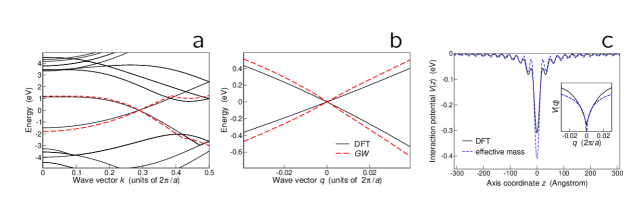
Figure 2: Electronic properties from many-body perturbation theory. a, $GW$ (dashed lines) and DFT (solid lines) band structure of the armchair carbon nanotube (3,3). b, Zoom close to the Dirac point K. The momentum $q$ is referenced from K. c, Long-range part of electron-hole interaction $V(z)$ along the tube axis according to: DFT (solid line), effective-mass model (dashed line). Inset: interaction $V(q)$ in momentum space. $V$ is integrated over the mesh of the $q$ grid and projected onto the conduction and valence bands shown in panel b, with $\left|q\right|<0.09(2\pi)/a$. The graphene lattice constant is $a=2.46$ Å.

Results

Exciton binding and instability

For the sake of computational convenience we focus on the smallest (3,3) armchair tube, which was investigated several times from first principles[53, 54, 55, 56, 57, 58, 59, 60]. We first check whether the structural optimization of the tube might lead to deviations from the ideal cylindrical shape, affecting the electronic states. Full geometry relaxation (Methods) yields an equilibrium structure with negligible corrugation. Thus, contrary to a previous claim[60], corrugation cannot be responsible of gap opening. We find that the average length of C-C bonds along the tube axis, 1.431 Å, is shorter than around the circumference, 1.438 Å, in perfect agreement with the literature[53].

We use density functional theory (DFT) to compute the band structure (solid lines in Fig. 2a), which provides the expected[43] zero gap at the Dirac point K. In addition, we adopt the $G0W0$ approximation for the self-energy operator[44] to evaluate many-body corrections to Kohn-Sham eigenvalues. The highest valence and lowest conduction bands are shown as dashed lines. The zoom near K (Fig. 2b) shows that electrons remain massless, with their bands stretched by $\sim$ 28% with respect to DFT (farther from K the stretching is $\sim$ 13%, as found previously[56]). Since electrons and holes in these bands have linear dispersion, they cannot form a conventional Wannier exciton, whose binding energy is proportional to the effective mass. However, the screened e-h Coulomb interaction $V(z)$ along the tube axis, projected onto the same bands, has long range (Fig. 2c)—a remarkable effect of the topology of the tube holding even for vanishing gap. Consequently, $V(q)$ exhibits a singularity in reciprocal space at $q=0$ (smoothed by numerical discretization in the inset of Fig. 2c), which eventually binds the exciton.

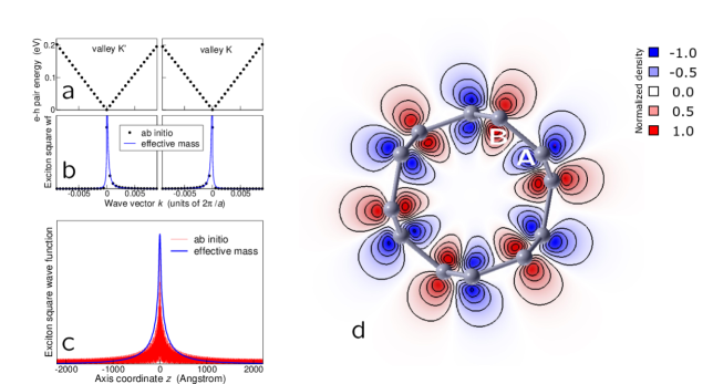
Figure 3: Wave function of the lowest-energy exciton of the (3,3) tube. a, $GW$ excitation spectrum of free e-h pairs with zero center-of-mass momentum in the two Dirac valleys. b, Square modulus of the triplet exciton wave function vs momentum $k$. Both first-principles (dots) and effective-mass (solid lines) probability weights accumulate asymmetrically close to Dirac points. The effective-mass model includes the dressed long-range interaction, the short-range intervalley exchange, and the small asymmetry of Dirac cones (cf. Supplementary Notes 1-3; a previous phenomenological theory[61] by one of the authors, which ignored the key-role of long-range interaction, is ruled out by the present work). c, Square modulus of the triplet exciton wave function vs e-h distance along the axis, $z$, according to first-principles (red curve) and effective-mass (blue curve) calculations. The Bohr diameter is larger than 2 $\mu$m. d, Cross-sectional contour map of the transition density of the singlet exciton, $\varrho_{\text{tr}}(\mathbf{r})$, obtained from first principles. The blue / red colour points to the deficit / surplus of charge, the isolines are equally spaced, the normalization of $\varrho_{\text{tr}}(\mathbf{r})$ is such that its maximum value is one, and letters label sublattices.

We solve the Bethe-Salpeter equation over an ultradense grid of 1800 $k$-points, which is computationally very demanding but essential for convergence. We find several excitons with negative excitation energies $\varepsilon_{\text{u}}$, in the range of 1–10 meV (Table 1).

	Triplet	Singlet
Lowest	-7.91	-6.10
1st excited	-6.40	-5.10
2st excited	6.65	8.82

Table 1: Excitation energies $\varepsilon_{\text{u}}$ of low-lying excitons of the (3,3) tube obtained from first-principles many-body perturbation theory in units of meV.

The exciton spectral weight is concentrated in a tiny neighbourhood of K and K^′ points in reciprocal space (Fig. 3b), hence the excitons are extremely shallow, spread over microns along the axis (Fig. 3c). Only e-h pairs with negative $k$ in valley K and positive $k$ in valley K^′ contribute to the exciton wave function, which is overall symmetric under time reversal but not under axis reflection within one valley, $k\rightarrow-k$, as shown in Fig. 3b (the axis origin is at Dirac point). On the contrary, the wave functions of excitons reported so far in nanotubes[36, 56, 37] are symmetric in $k$-space. The reason of this unusual behavior originates from the vanishing energy gap, since then e-h pairs cannot be backscattered by Coulomb interaction due to the orthogonality of initial and final states[62]. In addition, pair energies are not degenerate for $k\rightarrow-k$, as Dirac cones are slightly asymmetric (Supplementary Discussion and Supplementary Fig. 10).

The exciton with the lowest negative $\varepsilon_{\text{u}}$ makes the system unstable against the EI. The transition density, $\varrho_{\text{tr}}(\mathbf{r})=\left<\text{u}\right|\hat{\varrho}(\mathbf{r})\left|0\right>$, hints at the broken symmetry of the reconstructed ground state, as it connects the noninteracting ground state, $\left|0\right>$, to the exciton state, $\left|\text{u}\right>$, through the charge fluctuation operator $\hat{\varrho}$ (Fig. 3d). Here we focus on the simpler charge order (spin singlet excitons) and neglect magnetic phenomena (spin triplet), as the only relevant effect of spin-orbit coupling in real tubes[63, 64] is to effectively mix both symmetries. Figure 3d may be regarded as a snapshot of the polarization charge oscillation induced by the exciton, breaking the inversion symmetry between carbon sublattices A and B. Note that this originates from the opposite symmetries of $\left|0\right>$ and $\left|\text{u}\right>$ under A $\leftrightarrow$ B inversion and not from the vanishing gap. This charge displacement between sublattices is the generic signature of the EI, as its ground state may be regarded as a BCS-like condensate of excitons $\left|\text{u}\right>$ (see the formal demonstration in Supplementary Note 5).

Broken symmetry of the excitonic insulator

We use quantum Monte Carlo to verify the excitonic nature of the many-body ground state, by defining an order parameter characteristic of the EI, $\varrho_{\text{AB}}$. In addition, we introduce an alternative order parameter, $\varrho_{\text{Transl}}$, peculiar to a dimerized charge density wave (CDW) similar to the Peierls CDW predicted by some authors[57, 58, 59] for the smallest armchair tubes. The EI order parameter measures the uniform charge displacement between A and B sublattices, $\varrho_{\text{AB}}=(\sum_{i\in\text{A}}n_{i}-\sum_{i\in\text{B}}n_{i})/N_{\text{atom}}$, whereas $\varrho_{\text{Transl}}$ detects any deviation from the periodicity of the undistorted structure by evaluating the charge displacement between adjacent cells, $\varrho_{\text{Transl}}=\sum_{i}n_{i}(-1)^{i_{z}}/N_{\text{atom}}$ (Figs. 4b-e). Here the undistorted structure is made of a unit cell of twelve C atoms repeated along the $z$ direction with a period of 2.445 Å and labeled by the integer $i_{z}$, $n_{i}$ is the operator counting the electrons within a sphere of radius 1.3 a.u. around the $i$th atom, and $N_{\text{atom}}$ is the total number of atoms in the cluster. Both order parameters $\varrho_{\text{AB}}$ and $\varrho_{\text{Transl}}$ vanish in the symmetric ground state of the undistorted structure, which is invariant under sublattice-swapping inversion and translation symmetries.

Figure 4: Broken symmetry of the ground state from quantum Monte Carlo. a, The square of the charge displacement per atom (empty circles and squares for ‘AB’ and ‘Transl’ order parameters, respectively) is plotted vs the inverse of the number of atoms, $N_{\text{atom}}$, as obtained by variational (VMC) and lattice-regularized diffusion (LRDMC) quantum Monte Carlo. The filled symbols are linear extrapolations to the $N_{\text{atom}}=\infty$ limit. The error bars are estimated by means of the jackknife method using more than 30 independent samples for each independent twist (Methods). The error bars of empty symbols are not visible on the scale of the plot. b-e, The sketches of the tube illustrate the two possible broken symmetries, with the blue / red colour pointing to the deficit / surplus of charge. The AB order parameter, peculiar to the EI, is a uniform charge displacement between the two carbon sublattices (panels b and c show respectively the lateral and cross-sectional views of the tube). The Transl parameter is a charge displacement between two adjacent unit cells, signaling a charge density wave order breaking the translational symmetry (panels d and e).

We then perform variational Monte Carlo (VMC), using a correlated Jastrow-Slater ansatz that has proved[65] to work well in 1D correlated systems (Methods), as well as it is able to recover the excitonic correlations present in the mean-field EI wave function[2, 3, 4, 5] (Supplementary Discussion). We plot VMC order parameters in Fig. 4a. Spontaneously broken symmetry occurs in the thermodynamic limit if the square order parameter, either $\varrho_{\text{AB}}^{2}$ or $\varrho_{\text{Transl}}^{2}$, scales as $1/N_{\text{atom}}$ and has a non vanishing limit value for $N_{\text{atom}}\rightarrow\infty$. This occurs for $\varrho_{\text{AB}}^{2}$ (black circles in Fig. 4a), confirming the prediction of the EI, whereas $\varrho_{\text{Transl}}^{2}$ vanishes (red squares), ruling out the CDW instability (see Supplementary Discussion as well as the theoretical literature[57, 58, 52, 59] for the Peierls CDW case). We attribute the simultaneous breaking of sublattice symmetry and protection of pristine translation symmetry to the effect of long-range interaction.

The vanishing of $\varrho_{\text{Transl}}$ validates the ability of our finite-size scaling analysis to discriminate between kinds of order in the bulk. Though the value of $\varrho_{\text{AB}}$ after extrapolation is small, $\varrho_{\text{AB}}=0.0165\pm 0.0007$, it is non zero within more than twenty standard deviations. Besides, the quality of the fit of Fig. 4a appears good, because the data for the five largest clusters are compatible with the linear extrapolations of both $\varrho_{\text{AB}}^{2}$ and $\varrho_{\text{Transl}}^{2}$ within an acceptable statistical error. The more accurate diffusion Monte Carlo (LRDMC) values (obtained with the lattice regularization), shown in Fig. 4a as blue circles, confirm the accuracy of the variational calculation. However, as their cost is on the verge of present supercomputing capabilities, we were unable to treat clusters larger that $N_{\text{atom}}=48$, hence the statistical errors are too large to support a meaningful non zero value in the thermodynamic limit. Nevertheless, we obtain a non zero LRDMC value smaller than the one estimated by VMC but compatible with it within a few standard deviations.

Trends

As the extension of our analysis to systems larger than the (3,3) tube is beyond reach, we design an effective-mass theory to draw conclusions about trends in the armchair tube family, in agreement with first-principles findings. We solve the minimal Bethe-Salpeter equation for the massless energy bands $\varepsilon(k)=\pm\gamma\left|k\right|$ (Fig. 2b and Supplementary Note 1) and the long-range Coulomb interaction $V(q)$, the latter diverging logarithmically in one dimension for small momentum transfer $q$, $V(q)=(2e^{2}/A\kappa_{\text{r}})\ln(\left|q\right|R)$ (inset of Fig. 2c and Supplementary Note 2). Here $\gamma$ is graphene tight-binding parameter including $GW$ self-energy corrections, $k$ is the wave vector along the axis, $A$ is the tube length, $R$ is the radius, and $\kappa_{\text{r}}$ accounts for screening beyond the effective-mass approximation. By fitting the parameters $\gamma=0.5449$ eV$\cdot$nm and $\kappa_{\text{r}}=10$ to our first-principles data, we obtain a numerical solution of Bethe-Salpeter equation recovering approximately 60% of the lowest exciton energy $\varepsilon_{\text{u}}$ reported in Table 1 (Supplementary Note 3). Moreover, the wave function agrees with the one obtained from first principles (Fig. 3b, c). Importantly, $\varepsilon_{\text{u}}$ smoothly converges in an energy range that—for screened interaction—is significantly smaller than the extension of the Dirac cone, with no need of ultraviolet cutoff (Supplementary Fig. 9). Therefore, the exciton has an intrinsic length (binding energy), which scales like $R$ ($1/R$).

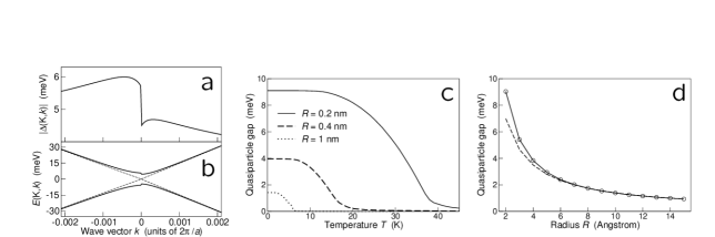
Figure 5: Excitonic insulator behaviour from mean-field theory. a, Excitonic order parameter, $\left|\Delta(\tau=\text{K},k)\right|$, vs momentum $k$ within K valley and (b) corresponding quasiparticle dispersion, $E(\text{K},k)$, for the (3,3) armchair carbon nanotube. The data are derived by solving self-consistently the gap equation. For comparison, the noninteracting bands are indicated (dashed lines). The band in the K^′ valley is obtained by time reversal, as $\left|\Delta(\text{K}^{\prime},k)\right|=\left|\Delta(\text{K},-k)\right|$. c, Quasiparticle gap vs temperature $T$ for different radii [for the (3,3) tube $R=2$ Å]. d, Quasiparticle gap vs $R$. The dashed curve is a fit proportional to $1/R$ pointing to the scaling behaviour at large $R$.

We adopt a mean-field theory of the EI as we expect the long-range character of excitonic correlations to mitigate the effects of quantum fluctuations. The EI wave function can be described as

$$\left|\Psi_{\text{EI}}\right>=\prod_{\sigma\sigma^{\prime}\tau k}\left[u_{\tau k}+\chi_{\sigma\sigma^{\prime}}v_{\tau k}e^{i\eta}\,\hat{c}^{\tau+}_{k,\sigma}\hat{v}^{\tau}_{k,\sigma^{\prime}}\right]\left|0\right>.$$ (1)

Here $\left|0\right>$ is the zero-gap ground state with all valence states filled and conduction states empty, the operator $\hat{c}^{\tau+}_{k,\sigma}$ ($\hat{v}^{\tau+}_{k,\sigma}$) creates an electron in the conduction (valence) band with wave vector $k$, spin $\sigma$, valley $\tau=$ K or K^′, $\eta$ is an arbitrary phase, and the $2\times 2$ matrix $\chi_{\sigma\sigma^{\prime}}$ discriminates between singlet and triplet spin symmetries of the e-h pair $\hat{c}^{\tau+}_{k,\sigma}\hat{v}^{\tau}_{k,\sigma^{\prime}}\left|0\right>$ (Fig. 1b). The positive variational quantities $u_{\tau k}$ and $v_{\tau k}$ are the population amplitudes of valence and conduction levels, respectively, with $u_{\tau k}^{2}+v_{\tau k}^{2}=1$. Whereas in the zero-gap state $u_{\tau k}=1$ and $v_{\tau k}=0$, in the EI state both $u_{\tau k}$ and $v_{\tau k}$ are finite and ruled by the EI order parameter $\Delta(\tau k)$, according to $u_{\tau k}\,v_{\tau k}=\left|\Delta(\tau k)\right|/2E(\tau k)$, with $E(\tau k)=[\varepsilon(\tau k)^{2}+\left|\Delta(\tau k)\right|^{2}]^{1/2}$. The parameter $\Delta(\tau k)$ obeys the self-consistent equation

$$\left|\Delta(\tau k)\right|=\sum_{\tau^{\prime}q}V^{\tau\tau^{\prime}}\!(k,k+q)\,u_{\tau^{\prime}k+q}\,v_{\tau^{\prime}k+q},$$ (2)

which is solved numerically by recursive iteration (here $V$ includes both long- and short-range interactions as well as form factors, see Supplementary Note 4). As shown in Fig. 5a, in each valley $\left|\Delta(\tau k)\right|$ is asymmetric around the Dirac point, a consequence of the peculiar character of the exciton wave function of Fig. 3b. The electrons or holes added to the neutral ground state are gapped quasiparticle excitations of the EI, whose energy bands $\pm E(\tau k)$ are shown in Fig. 5b. The order parameter at the Dirac point, $\left|\Delta(\tau,k=0)\right|$, is half the many-body gap. This gap is reminescent of the exciton binding energy, since in the ground state all electrons and holes are bound, so one needs to ionize an exciton-like collective state to create a free electron-hole pair. The gap strongly depends on temperature, with a low-temperature plateau, a steep descent approaching the critical temperature, and a milder tail (Fig. 5c). The gap approximately scales as $1/R$ for different tubes (circles in Fig. 5d): whereas at large $R$ such scaling is exact (cf. dashed curve), at small $R$ the gap is enhanced by short-range intervalley interaction (the decay of $\Delta$ will be mitigated if $\kappa_{\text{r}}$ is sensitive to $R$).

In experiments, many-body gaps are observed in undoped, ultraclean suspended tubes[66], whereas Luttinger liquid signatures emerge in doped tubes[43, 35]. Though it is difficult to compare with the measured many-body gaps[66], as the chiralities of the tubes are unknown and the radii estimated indirectly, the measured range of 10–100 meV is at least one order of magnitude larger than our predictions. By doping the tube, we expect that the enhanced screening suppresses the EI order, quickly turning the system into a Luttinger liquid. We are confident that advances in electron spectroscopies will allow to test our theory.

The broken symmetry associated with the EI ground state depends on the exciton spin[5]. For spin singlet ($\chi_{\sigma\sigma^{\prime}}=\delta_{\sigma\sigma^{\prime}}$) and order parameter real ($\eta=0,\pi$), $\left|\Psi_{\text{EI}}\right>$ breaks the charge symmetry between A and B carbon sublattices. The charge displacement per electron, $\Delta e/e$, at each sublattice site is

$$\frac{\Delta e}{e}=\pm\cos{\eta}\frac{a}{A}\sum_{\tau k}\frac{\left|\Delta(\tau k)\right|}{2E(\tau k)},$$ (3)

where the positive (negative) sign refers to the A (B) sublattice (Supplementary Note 6). For the (3,3) tube this amounts to $\varrho_{\text{AB}}=0.0068$, which compares well with Monte Carlo estimates of 0.0067 and 0.0165 from LRDMC and VQMC, respectively. Note that assessing the energy difference between EI and zero-gap ground states is beyond the current capability of quantum Monte Carlo: the mean-field estimate of the difference is below 10^-6 Hartree per atom, which is less than the noise threshold of the method (10^-5 Hartree per atom).

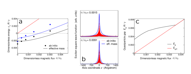
Figure 6: Effect of an axial magnetic field. a, Excitation energies, $\varepsilon_{\text{u}}R/\gamma$, of low-lying excitons vs magnetic flux, $\phi/\phi_{0}$. Both first-principles (dots) and effective-mass (solid lines) data are reported. The black (blue) colour labels the triplet (singlet) spin symmetry. The red line is the noninteracting gap and the dashed line is the instability threshold. b, Square modulus of the wave function of the lowest exciton vs e-h distance along the axis, $z$, for increasing values of magnetic flux. Both ab initio (red lines) and effective-mass (blue lines) data are reported. c, Total quasiparticle gap $E_{\text{g}}R/\gamma$ vs $\phi/\phi_{0}$. This observable may be accessed through Coulomb blockade spectroscopy. The red line is the noninteracting gap, $E_{\text{g},0}$.

Effect of magnetic field

The EI is sensitive to the opening of a noninteracting gap, $E_{\text{g},0}$, tuned by the magnetic field parallel to the tube axis, $B$. The ratio of the flux piercing the cross section, $\phi=\pi R^{2}B$, to the flux quantum, $\phi_{0}=ch/e$, amounts to an Aharonov-Bohm phase displacing the position of the Dirac point along the transverse direction[67], $k_{\perp}=(\phi/\phi_{0})R^{-1}$. Consequently, $E_{\text{g},0}=2\gamma\left|k_{\perp}\right|$ is linear with $\phi/\phi_{0}$ (red line in Fig. 6a, c). Figure 6a shows the evolution of low-lying singlet (blue lines) and triplet (black lines) excitons of the (3,3) tube. In addition, we have implemented a full first-principles description of $B$ building on a previous method[68]. First-principles (circles) and model (solid lines) calculations show a fair agreement, which validates the effective-mass theory since all free parameters have been fixed at zero field. Here we rescale energies by $R/\gamma$ since we expect the plot to be universal, except for small corrections due to short-range interactions. Excitation energies obtained within the effective-mass model crossover from a low-field region, where $\varepsilon_{\text{u}}$ is almost constant, to a high-field region, where $\varepsilon_{\text{u}}$ increases linearly with $\phi/\phi_{0}$. Exciton wave functions are effectively squeezed by the field in real space (Fig. 6b), whereas in reciprocal space they loose their asymmetric character: the amplitudes become evenly distributed around the Dirac points (Supplementary Discussion and Fig. 11) and similar to those reported in literature[36, 56, 37]. At a critical flux $\phi_{\text{c}}/\phi_{0}\approx 0.035$ the excitation energy $\varepsilon_{\text{u}}$ becomes positive, hence the tube exits the EI phase and $\Delta$ vanishes in a BCS-like fashion. We point out that the critical field intensity, $B_{\text{c}}\approx 460$ T $\cdot(R$ [Å]$)^{-2}$, is out of reach for the (3,3) tube but feasible for larger tubes. The total transport gap, $E_{\text{g}}=(E_{\text{g},0}^{2}+4\left|\Delta\right|^{2})^{1/2}$, first scales with $\phi/\phi_{0}$ as $E_{\text{g},0}$, then its slope decreases up to the critical threshold $\phi_{\text{c}}/\phi_{0}$, where the linear dependence on $\phi/\phi_{0}$ is restored (Fig. 6c). This behaviour is qualitatively similar to that observed by Coulomb blockade spectroscopy in narrow-gap tubes close to the ‘Dirac’ value of $B$, which counteracts the effect of $E_{\text{g},0}$ on the transport gap, fully suppressing the noninteracting contribution[66].

Discussion

The observed[66] many-body gap of armchair tubes was attributed to the Mott insulating state. The system was modeled as a strongly interacting Luttinger liquid with a gap enforced by short-range interactions[46, 49], whereas the long tail of the interaction was cut off at an extrinsic, setup-dependent length[47, 48, 50, 51, 52]. This model thus neglects the crucial effect of long-range interaction, which was highlighted in Fig. 1: Were any cutoff length smaller than the intrinsic exciton length, which is micrometric and scales with $R$, excitons could not bind.

Whereas armchair carbon nanotubes are regarded as quintessential realizations of the Luttinger liquid, since their low-energy properties are mapped into those of two-leg ladders[46], we emphasize that this mapping is exact for short-range interactions only. Among e-h pair collective modes with total momentum $q=0$, Luttinger liquid theory routinely describes plasmons[69] but not excitons. Contrary to conventional wisdom, armchair tubes are EIs.

The excitonic and Mott insulators are qualitatively different. The EI exhibits long-range charge order, which does not affect the translational symmetry of the zero-gap tube. In the Mott insulator, charge and spin correlations may or may not decay, but always add a $2\pi/(2k_{\text{F}})$ [or $2\pi/(4k_{\text{F}})$] periodicity to the pristine system, $k_{\text{F}}$ being the Fermi wave vector[50, 51]. The EI gap scales like $1/R$ (Fig. 5d), the Mott gap like $1/R^{1/(1-g)}$, with predicted[47, 50, 51, 52] values of $g$ pointing to a faster decay, $g<1$. The EI order parameter is suppressed at high temperature (Fig. 5c) and strong magnetic field (Fig. 6c); the Mott gap is likely independent of both fields (the Aharonov-Bohm phase does not affect Hubbard-like Coulomb integrals). Importantly, the EI gap is very sensitive to the dielectric environment[70], whereas the Mott gap is not. This could explain the dramatic variation of narrow transport gaps of suspended tubes submerged in different liquid dielectrics[42].

We anticipate that armchair tubes exhibit an optical absorption spectrum in the THz range dominated by excitons, which provides an independent test of the EI phase. Furthermore, we predict they behave as ‘chiral electronic ferroelectrics’, displaying a permanent electric polarization $\mathbf{P}$ of purely electronic origin[7], whereas conventional ferroelectricity originates from ionic displacements. In fact, the volume average of $\mathbf{P}$ is zero but its circulation along the tube circumference is finite. Therefore, a suitable time-dependent field excites the ferroelectric resonance[7] associated with the oscillation of $\mathbf{P}$. The special symmetry of armchair tubes[62] is expected to protect this collective (Goldstone) mode of oscillating electric dipoles from phase-locking mechanisms. The resulting soft mode—a displacement current along the tube circumference—is a manifestation of the long-debated[71, 72, 6, 7, 9, 8, 10, 11] exciton superfluidity.

In conclusion, our calculations demonstrated that an isolated armchair carbon nanotube at charge neutrality is an excitonic insulator, owing to the strong e-h binding in quasi-1D, and the almost unscreened long-range interactions. The emergence of this exotic state of matter, predicted fifty years ago, does not fit the common picture of carbon nanotubes as Luttinger liquids. Our first-principles calculations provide tests to discriminate between the excitonic insulator and the Luttinger liquid at strong coupling, the Mott insulator state. We expect a wide family of narrow-gap carbon nanotubes to be excitonic insulators. Carbon nanotubes are thus invaluable systems for the experimental investigation of this phase of matter.

0.1 Many-body perturbation theory from first principles.

The ground-state calculations for the (3,3) carbon nanotube were performed by using a DFT approach, as implemented in the Quantum ESPRESSO package[73]. The generalized gradient approximation (GGA) PW91 parametrization[74] was adopted together with plane wave basis set and norm-conserving pseudopotentials to model the electron-ion interaction. The kinetic energy cutoff for the wave functions was set to 70 Ry. The Brillouin zone was sampled by using a 200 $\times$ 1 $\times$ 1 $k$-point grid. The supercell side perpendicular to the tube was set to 38 Bohr and checked to be large enough to avoid spurious interactions with its replica.

Many-body perturbation theory[44] calculations were performed using the Yambo code[75]. Many-body corrections to the Kohn-Sham eigenvalues were calculated within the $G0W0$ approximation to the self-energy operator, where the dynamic dielectric function was obtained within the plasmon-pole approximation. The spectrum of excited states was then computed by solving the Bethe-Salpeter equation (BSE). The static screening in the direct term was calculated within the random-phase approximation with inclusion of local field effects; the Tamm-Dancoff approximation for the BSE Hamiltonian was employed after having verified that the correction introduced by coupling the resonant and antiresonant part was negligible. Converged excitation energies, $\varepsilon_{\text{u}}$, were obtained considering respectively 3 valence and 4 conduction bands in the BSE matrix. For the calculations of the $GW$ band structure and the Bethe-Salpeter matrix the Brillouin zone was sampled with a 1793 $\times$ 1 $\times$ 1 $k$-point grid. A kinetic energy cutoff of 55 Ry was used for the evaluation of the exchange part of the self energy and 4 Ry for the screening matrix size. Eighty unoccupied bands were used in the integration of the self-energy.

The effect of the magnetic field parallel to the axis on the electronic structure of the nanotube ground state (eigenvalues and eigenfunctions) was investigated following the method by Sangalli & Marini[68]. For each value of the field, the eigenvalues and eigenfunctions were considered to build the screening matrix and the corresponding excitonic Hamiltonian.

To obtain the equilibrium structure, we first considered possible corrugation effects. We computed the total energy for a set of structures obtained by varying the relative positions of A and B carbon atoms belonging to different sublattices, so that they were displaced one from the other along the radial direction by the corrugation length $\Delta$ and formed two cylinders, as in Fig. 1(b) of Lu et al.[60]. Then, we fitted the total energy per carbon atom with an elliptic paraboloid in the two-dimensional parameter space spanned by $\Delta$ and the carbon bond length. In agreement with Lu et al.[60], we find a corrugated structure with a bond length of 1.431 Å and a corrugation parameter $\Delta=0.018$ Å. Eventually, starting from this structure, we performed a full geometry relaxation of the whole system allowing all carbon positions to change until the forces acting on all atoms became less than 5$\cdot 10^{-3}$ eV$\cdot$Å^-1. After relaxation, the final structure presents a negligible corrugation ($\Delta<10^{-5}$ Å) and an average length of C-C bonds along the tube axis, 1.431 Å, slightly shorter than the C-C bonds around the tube circumference, 1.438 Å. The average radius and translation vector of the tube are respectively 2.101 Å and 2.462 Å, in perfect agreement with the literature[53]. The obtained equilibrium coordinates of C atoms in the unitary cell are shown in Supplementary Table 1.

0.2 Quantum Monte Carlo method.

We have applied the quantum Monte Carlo method to carbon nanotubes by using standard pseudopotentials for the 1$s$ core electrons of the carbon atom[76]. We minimize the total energy expectation value of the first-principles Hamiltonian, within the Born-Oppheneimer approximation, by means of a correlated wave function, $J\left|\text{SD}\right>$. This is made of a Slater determinant, $\left|\text{SD}\right>$, defined in a localized GTO VDZ basis[76] ($5s5p1d$) contracted into six hybrid orbitals per carbon atom[77], multiplied by a Jastrow term, $J$. The latter, $J=J_{1}J_{2}$, is the product of two factors: a one-electron one term, $J_{1}=\prod_{i}\exp{\!\left[u_{\text{1body}}(\textbf{r}_{i})\right]}$, and a two-electron correlation factor, $J_{2}=\prod_{i<j}\exp{\!\left[u(\textbf{r}_{i},\textbf{r}_{j})\right]}$. The two-body Jastrow factor $J_{2}$ depends explicitly on the $N_{\text{e}}$ electronic positions, $\{\textbf{r}_{i}\}$, and, parametrically, on the $N_{\text{C}}$ carbon positions, $\textbf{R}_{I}$, $I=1,\cdots N_{\text{C}}$. The pseudopotential functions, $u$ and $u_{\text{1body}}$, are written as:

$$u(\textbf{ r},\textbf{ r}^{\prime})=u_{\text{ee}}(|\textbf{ r}-\textbf{ r}^{\prime}|)+\sum_{\mu>0,\nu>0}u_{\mu\nu}\,\chi_{\mu}(\textbf{r})\chi_{\nu}(\textbf{r}^{\prime}),$$ (4)

$$u_{\text{1body}}(\textbf{r})=\sum_{\mu>0}u_{\mu 0}\,\chi_{\mu}(\textbf{r}),$$ (5)

where $u_{\text{ee}}=2^{-1}r/(1+b_{\text{ee}}r)$ is a simple function, depending on the single variational parameter $b_{\text{ee}}$, which allows to satisfy the electron-electron cusp condition, and $u_{\mu\nu}$ is a symmetric matrix of finite dimension. For non-null indices, $\mu,\nu>0$, the matrix $\bm{u}$ describes the variational freedom of $J_{2}$ in a certain finite atomic basis, $\chi_{\mu}(\textbf{r})$, which is localized around the atomic centers $\textbf{R}_{I(\mu)}$ and is made of $3s2p$ GTO orbitals per atom. Note that the one-body Jastrow term $J_{1}$ is expanded over the same atomic basis and its variational freedom is determined by the first column of the matrix, $u_{\mu 0}$.

We use an orthorombic unit cell $L_{x}\times L_{y}\times L_{z}$ containing twelve atoms with $L_{x}=L_{y}=36$ Å and $L_{z}=2.445$ Å. This cell is repeated along the $z$ direction for $n=1,2,3,4,5,6$ times, up to $72$ carbon atoms in the supercell. Periodic images in the $x$ and $y$ directions are far enough that their mutual interaction can be safely neglected. Conversely, in the $z$ direction we apply twisted periodic boundary conditions and we integrate over that with a number $n_{\theta}$ of twists, $n_{\theta}=80,40,30,20,20,20$ for $n=1,2,3,4,5,6$, respectively, large enough to have converged results for each supercell.

The initial Slater determinant was taken by performing a standard LDA calculation. The molecular orbitals, namely their expansion coefficients in the GTO localized basis set, as well as the matrix $\bm{u}$ determining the Jastrow factor, were simultaneously optimized with well established methods developed in recent years[78, 79], which allows us to consider up to $3000$ independent variational parameters in a very stable and efficient way. Note that the two-body Jastrow term $J_{2}$ can be chosen to explicitly recover the EI mean-field wave function (1), as shown in Supplementary Discussion. After the stochastic optimization the correlation functions / order parameters can be computed in a simple way within variational Monte Carlo (VMC).

We also employ lattice regularized diffusion Monte Carlo (LRDMC) within the fixed-node approximation, using a lattice mesh of $a_{\text{mesh}}=0.2$ and $a_{\text{mesh}}=0.4$ a.u., respectively, in order to check the convergence for $a_{\text{mesh}}\to 0$. The fixed-node approximation is necessary for fermions for obtaining statistically meaningful ground-state properties. In this case the correlation functions / order parameters, depending only on local (i.e., diagonal in the basis) operators, such as the ones presented in this work, are computed with the forward walking technique[80], which allows the computation of pure expectation values on the fixed-node ground state.

Code availability

Many-body perturbation theory calculations were performed by means of the codes Yambo (http://www.yambo-code.org/) and Quantum ESPRESSO (http://www.quantum-espresso.org), which are both open source software. Quantum Monte Carlo calculations were based on TurboRVB code (http://trac.sissa.it/svn/TurboRVB), which is available from S.S. upon reasonable request (email: sorella@sissa.it).

Data availability

The data that support the findings of this study are available from the corresponding author upon reasonable request.

Supplementary Note 1

Effective-mass theory of armchair carbon nanotubes

In this Note we recall the effective-mass theory of electronic $\pi$-states in single-wall carbon nanotubes, focusing on the lowest conduction and highest valence band of undoped armchair tubes[67, 81, 61]. Carbon nanotubes may be thought of as wrapped sheets of graphene, hence nanotube electronic states are built from those of graphene through a folding procedure, after quantizing the transverse wave vector. Low-energy graphene states belong to one of the two Dirac cones, whose apexes intersect the degenerate K and K^′ points, respectively, at the corners of graphene first Brillouin zone. At these two points the energy gap is zero.

Close to Brillouin zone corners $\tau=\text{K},\text{K}^{\prime}$, a nanotube state $\psi(\mathbf{r})$ is the superposition of slowly-varying envelope functions $F^{\tau\eta}\!(\mathbf{r})$ multiplied by the Bloch states $\psi_{\tau\eta}(\mathbf{r})$, the latter having two separate components localized on sublattices $\eta=A$ and $\eta=B$, respectively (cyan and red dots in Supplementary Fig. 1):

$$\psi(\mathbf{r})=\sum_{\tau=\text{K},\text{K}^{\prime}}\sum_{\eta=A,B}F^{\tau\eta}\!(\mathbf{r})\,\psi_{\tau\eta}(\mathbf{r}).$$ (6)

The effective-mass approximation of Supplementary Eq. (6) goes beyond the usual one-valley treatment, as below we explicitly consider intervalley coupling due to Coulomb interaction. The relative phases of different Bloch state components $\psi_{\tau\eta}$ are fixed by symmetry considerations, as detailed in Supplementary Note 7. The envelope $F^{\tau\eta}$ is a pseudospinor with respect to valley and sublattice indices, $\bm{F}\equiv(F^{\text{K}A},F^{\text{K}B},F^{\text{K}^{\prime}A},F^{\text{K}^{\prime}B})^{T}$. In the valley-sublattice product space, $\bm{F}$ obeys the Dirac equation of graphene:

$$\gamma\left[\bm{\sigma}_{x}\otimes\bm{1}_{\tau}\hat{k}_{x}+\bm{\sigma}_{y}\otimes\bm{\tau}_{z}\hat{k}_{y}\right]\bm{F}(\mathbf{r})=\varepsilon\,\bm{F}(\mathbf{r}).$$ (7)

Here $\bm{\sigma}_{x}$ and $\bm{\sigma}_{y}$ are 2 $\times$ 2 Pauli matrices acting on the sublattice pseudospin, $\bm{\tau}_{z}$ and the 2 $\times$ 2 identity matrix $\bm{1}_{\tau}$ act on the valley pseudospin, $\hat{k}_{x}=-i\partial/\partial x$ is is the wave vector operator along the circumference direction $x$ and $\hat{k}_{y}=-i\partial/\partial y$ acts on the tube axis coordinate $y$, $\gamma$ is graphene’s band parameter, and $\varepsilon$ is the single-particle energy. Furthermore, $\bm{F}$ obeys the boundary condition along the tube circumference:

$$\bm{F}(\mathbf{r+L})=\bm{F}(\mathbf{r})\exp\left(2\pi i\,\varphi\right),$$ (8)

where $\mathbf{L}$ is the chiral vector in the circumference direction of the tube and $\left|\mathbf{L}\right|=L=2\pi R$ is the circumference. A magnetic field may or may not be applied along the tube axis, with $\varphi=\phi/\phi_{0}$ being the ratio of the magnetic flux $\phi$ piercing the tube cross section to the magnetic flux quantum $\phi_{0}=ch/e$. Supplementary Eq. (7) depends on the reference frame. Note that in our effective-mass treatment the $x$ and $y$ directions are parallel to the circumference and axis of the tube, respectively, as shown in Supplementary Fig. 1a, whereas in the main text as well as in the first-principles treatment the $z$ axis is parallel to the tube.

Supplementary Fig. 1 Carbon nanotube reference frames for the effective-mass model. a Reference frame for the armchair tube used in this work. The $x$ and $y$ directions are parallel to the circumference and axis of the tube, respectively. The small vector is $\mathbf{R}_{0}^{B}$, i.e., the basis vector locating the origin of the B sublattice. Cyan and red dots point to A and B sublattices, respectively. b Ando’s reference frame for a generic tube. The frame origin is located on an atom of the B sublattice. The tube frame is obtained by rotating the $x^{\prime}y^{\prime}$ graphene reference frame by the chiral angle $\alpha$. The chiral vector $\mathbf{L}$ identifying the tube circumference is $\mathbf{L}=-m\mathbf{a}-(n+m)\mathbf{b}$ in terms of the conventional chiral indices $(n,m)$, where $\mathbf{a}$ and $\mathbf{b}$ are the primitive translation vectors of graphene shown in the picture. For an equivalent choice of $\mathbf{L}$ one has $\alpha=\pi/6$ for $(n,n)$ armchair tubes and $\alpha=0$ and for $(n,0)$ zigzag tubes. $a$ is the lattice constant of graphene.

The energy bands are specified by the valley index $\tau$, the valence index $\alpha=c$, $v$ denoting either the conduction ($\alpha=c$) or the valence band ($\alpha=v$), and the wave vector $k$ in the axis direction. The wave functions in K and K^′ valleys are respectively $\bm{F}\equiv(\bm{F}^{\text{K}}_{\alpha k}(\mathbf{r}),0)^{T}$ and $(0,\bm{F}^{\text{K}^{\prime}}_{\alpha k}(\mathbf{r}))^{T}$, with $\bm{F}^{\tau}_{\alpha k}(\mathbf{r})\equiv(F^{\tau A}_{\alpha k},F^{\tau B}_{\alpha k})^{T}$ being a plane-wave pseudospinor in the sublattice space,

$$\bm{F}^{\tau}_{\alpha k}(\mathbf{r})=\bm{\xi}^{\tau}_{\alpha k}(x)\frac{1}{\sqrt{A}}\exp{(iky)},$$ (9)

where $A$ is the tube length and the wave function $\bm{\xi}^{\tau}_{\alpha k}(x)$ for the motion along the circumference direction is

$$\bm{\xi}^{\tau}_{\alpha k}(x)=\frac{1}{\sqrt{L}}\exp{(ik_{\perp}x)}\bm{F}_{\tau\alpha k}.$$ (10)

The constant pseudospinor $\bm{F}_{\tau\alpha k}$ is a unit vector with a $k$-dependent phase between the two sublattice components,

$$\bm{F}_{\text{K}\alpha k}=\frac{1}{\sqrt{2}}{b(k)\choose s_{\alpha}},\qquad\bm{F}_{\text{K}^{\prime}\alpha k}=\frac{1}{\sqrt{2}}{b^{*}\!(k)\choose s_{\alpha}},$$ (11)

where

$$b(k)=\frac{k_{\perp}-ik}{\sqrt{k^{2}_{\perp}+k^{2}}},$$ (12)

and $s_{\alpha}=\pm 1$ for conduction and valence bands, respectively. In Supplementary Eqs. (10) and (12) the transverse wave vector $k_{\perp}$ is proportional to the magnetic flux $\varphi$,

$$k_{\perp}=\frac{\varphi}{R}.$$ (13)

In each valley, the energy is

$$\varepsilon_{\alpha}(k)=s_{\alpha}\gamma\sqrt{k^{2}_{\perp}+k^{2}},$$ (14)

where the origin of the $k$ axis is located at the Dirac point K (K^′).

Supplementary Fig. 2 $GW$ band structure of the (3,3) tube. a $GW$ band structure vs wave vector $k$ close to the Dirac point K. Red [grey] and black dots point to chirality indices ${\cal{C}}=+1$ and -1, respectively. b Electron-hole pair excitation energy vs $k$. The lines are linear fits to the data.

Figure 2a of main text shows the first-principles band structure of the (3,3) tube in a range of a few eV around the Dirac point, with $k$ scanning half Brillouin zone, between the origin ($k=0$, $\Gamma$ point) and $k=\pi/a$ ($a=2.46$ Å is graphene lattice constant). The negative $k$ axis, containing the K^′ point, is obtained by specular reflection. The DFT / $GW$ location of the Dirac point is K = 0.289 $(2\pi/a)$, whereas the effective-mass estimate is K = $1/3$ $(2\pi/a)$ (the discrepancy between DFT and tight-binding predictions is well documented in the literature[57, 58]). As seen in Supplementary Fig. 2a, the $GW$ bands are approximately linear in an energy range of at least $\pm$ 0.4 eV around the Dirac point, which validates the effective-mass model at low energy.

Note that, in the absence of the magnetic field, electron states have a well defined chirality[82, 62, 83], which is one of the two projections, $\cal{C}$, of the sublattice pseudospin onto the momentum direction, expressed as the eigenvalues ${\cal{C}}=\pm 1$ of the operator $\bm{\sigma}_{y}\otimes\bm{\tau}_{z}$. The chirality index is highlighted by red (${\cal{C}}=+1$) and black (${\cal{C}}=-1$) colour in Supplementary Fig. 2a.

Supplementary Note 2

Electron-electron interaction: Effective-mass vs first-principles description

Within the effective-mass framework, the Coulomb interaction $v$ between two electrons on the carbon nanotube cylindrical surface located at $\mathbf{r}\equiv(x,y)$ and $\mathbf{r}^{\prime}\equiv(x^{\prime},y^{\prime})$, respectively, is[81]

$$v(\mathbf{r},\mathbf{r}^{\prime})=\sum_{q}e^{iq(y-y^{\prime})}\frac{2e^{2}}{\kappa_{\text{r}}A}K_{0}\!\left(2R\left|q\sin{\!\left(\frac{x-x^{\prime}}{2R}\right)}\right|\right),$$ (15)

where $\kappa_{\text{r}}$ is a static dielectric constant that takes into account polarization effects due to the electrons not included in the effective-mass description plus the contribution of the dielectric background. The interaction matrix element between single-particle states is[84, 85]

$$V_{(\tau,\alpha,k+q),(\tau^{\prime},\beta^{\prime},k^{\prime});(\tau^{\prime},\alpha^{\prime},k^{\prime}+q)(\tau,\beta,k)}$$

$$\quad=\quad\int\!\!d\mathbf{r}\!\int\!\!d\mathbf{r}^{\prime}\;[\bm{F}^{\tau}_{\alpha k+q}(\mathbf{r})]^{\dagger}\!\cdot\!\bm{F}^{\tau}_{\beta k}(\mathbf{r})\,\,v(\mathbf{r},\mathbf{r}^{\prime})\;[\bm{F}^{\tau^{\prime}}_{\beta^{\prime}k^{\prime}}(\mathbf{r}^{\prime})]^{\dagger}\!\cdot\!\bm{F}^{\tau^{\prime}}_{\alpha^{\prime}k^{\prime}+q}(\mathbf{r}^{\prime})$$

$$\quad\quad=\quad\frac{1}{A}\,\bm{F}_{\tau\alpha k+q}^{\dagger}\!\cdot\!\bm{F}_{\tau\beta k}\,\,\,\bm{F}_{\tau^{\prime}\beta^{\prime}k^{\prime}}^{\dagger}\!\cdot\!\bm{F}_{\tau^{\prime}\alpha^{\prime}k^{\prime}+q}\,\,v(q),$$ (16)

where the one-dimensional effective interaction resolved in momentum space,

$$v(q)=\frac{2e^{2}}{\kappa_{\text{r}}}\,I_{0}\!\left(R\left|q\right|\right)\,K_{0}\!\left(R\left|q\right|\right),$$ (17)

is modulated by a form factor given by overlap terms between sublattice pseudospinors [$I_{0}(z)$ and $K_{0}(z)$ are the modified Bessel functions of the first and second kind, respectively[86]]. The effect of screening due to the polarization of those electrons that are treated within the effective-mass approximation is considered by replacing $v(q)$ with

$$w(q)=\frac{v(q)}{\varepsilon(q)}$$ (18)

in the matrix element (16), where $\varepsilon(q)$ is the static dielectric function (to discriminate between screened and unscreened matrix elements we use respectively ‘w’ and ‘v’ letters throughout the Supplementary Information). It may be shown that dynamical polarization effects are negligible in the relevant range of small frequencies, which is comparable to exciton binding energies.

Note that terms, similar to Supplementary Eq. (16), that scatter electrons from one valley to the other are absent in the effective mass approximation. These small intervalley terms, as well as the interband exchange terms, which are both induced by the residual, short-range part of Coulomb interaction, are discussed in Supplementary Note 3.

Effect of chiral symmetry. The chiralities of electron states, which is illustrated in Supplementary Fig. 3a (solid and dashed lines label ${\cal{C}}=+1$ and ${\cal{C}}=-1$, respectively), signficantly affects Coulomb interaction matrix elements. This occurs through the form factors of the type $\bm{F}^{\dagger}\!\cdot\!\bm{F}$ appearing in Supplementary Eq. (16), which are overlap terms between sublattice pseudospinors.

Supplementary Fig. 3 Effect of chirality on Coulomb interaction matrix elements. a Energy bands and chiralities of electron states in armchair carbon nanotubes in the absence of the magnetic field. Solid and dashed lines highlight chirality ${\cal{C}}=\pm 1$, respectively. b Allowed scattering processes induced by long-range Coulomb interaction. The indices $\tau=$ K, K^′ and $\alpha=c,v$ label valleys and bands, respectively. The chirality is conserved at each vertex of diagrams.

As apparent from their analytical structure,

$$\bm{F}_{\tau\alpha k+q}^{\dagger}\cdot\bm{F}_{\tau\beta k}=\frac{1}{2}\left[\,\text{sign}(k)\,\text{sign}(k+q)+s_{\beta}s_{\alpha}\right],$$ (19)

the chiral symmetry of the states is conserved at each vertex of Coulomb scattering diagrams (see Supplementary Fig. 3b), hence initial and final states scattered within the same band must have the same momentum direction. This significantly affects the Bethe-Salpeter equation for excitons, as we show below. We are especially interested in the dominant long-range Coulomb matrix element[5] that binds electrons and holes:

$$V_{(\tau,c,k+q),(\tau,v,k);(\tau,v,k+q)(\tau,c,k)}\equiv\frac{\tilde{V}(k+q,k)}{A}.$$ (20)

This term scatters electron-hole pairs from the initial pair state $(c,k)(v,k)$ to the final state $(c,k+q)(v,k+q)$ within the same valley $\tau$. Throughout this Supplementary Information we use the tilde symbol for quantities whose dimension is an energy multiplied by a length, like $V=\tilde{V}/A$.

In the first instance we neglect screening, since for low momentum transfer, $q\rightarrow 0$, polarization is suppressed hence $\varepsilon(q)\rightarrow 1$. In this limit Coulomb interaction diverges logarithmically,

$$v(q)\rightarrow-\frac{2e^{2}}{\kappa_{\text{r}}}\ln{\!\left(R\left|q\right|\right)},$$ (21)

but this is harmless to the Bethe-Salpeter equation, since $v(q)$ occurs only in the kernel of the scattering term, hence it is integrated over $q$ for macroscopic lengths $A$,

$$-\frac{1}{A}\sum_{q}\tilde{V}(k+q,k)\ldots\rightarrow-\frac{1}{2\pi}\int\!dq\,\tilde{V}(k+q,k)\ldots,$$ (22)

which removes the divergence. Note that, throughout this Supplementary Information and opposite to the convention of Fig. 2c of main text, we take $V$ as a positive quantity. In detail, we discretize the momentum space axis, $k\rightarrow k_{i}$, where $k_{i}=i2\pi/(Na)$, $i=-N/2+1,\ldots,0,1,\ldots,N/2$, $N=A/a$ is the number of unitary cells, and $\Delta k=2\pi/(Na)$ is the mesh used in the calculation. Hence, the regularized matrix element, integrated over the mesh, is

$$V(k_{j}+q_{i},k_{j})=\frac{1}{2\pi}\int_{q_{i}-\Delta k}^{q_{i}}\!\!\!\!dq\,\tilde{V}(k_{j}+q,k_{j}).$$ (23)

Supplementary Fig. 4 Dominant interband Coulomb matrix element in the $(k,k^{\prime})$ space close to the K point. a Effective-mass ‘bare’ matrix element $V(k,k^{\prime})$, with $\kappa_{\text{r}}=10$ and $\varepsilon(k-k^{\prime})=1$. The isolines of the two-dimensional contour map point to the heights of 4 and 8 meV, respectively. b Modulus of DFT screened matrix element $W^{\text{DFT}}(k,k^{\prime})$ obtained within the random phase approximation for the $(3,3)$ armchair tube. Here $N=900$ and K = $0.289(2\pi)/a$.

In Supplementary Fig. 4 we compare $V$ (panel a, $\kappa_{\text{r}}=10$) with the modulus of the screened DFT matrix element $W^{\text{DFT}}$ obtained for the $(3,3)$ tube (panel b). The two plots are three-dimensional contour maps in a square domain $(k,k^{\prime})$ centered around the Dirac point, with K = $0.289(2\pi)/a$ and $N=900$. The two matrix elements agree almost quantitatively, as they both exhibit: (i) zero or very small values in the second and fourth quadrants, i.e., $k>$ K and $k^{\prime}<$ K or $k<$ K and $k^{\prime}>$ K (ii) a logarithmic spike on the domain diagonal, i.e., $k^{\prime}\rightarrow k$. This behavior has a simple interpretation in terms of exciton scattering, as an electron-hole pair with zero center-of-mass momentum, $(c,k)(v,k)$, has a well-defined chirality with respect to the noninteracting ground state, i.e., $\Delta{\cal{C}}=+2=1-(-1)$ for $k>$ K ($\Delta{\cal{C}}=-2$ for $k<$ K). The chirality of the e-h pair is conserved during Coulomb scattering, i.e., as the pair changes its relative momentum from $2k=k-(-k)$ to $2k^{\prime}$.

Supplementary Fig. 5 Dominant interband Coulomb matrix elements vs $k$. Dominant interband Coulomb matrix elements $V(k,k_{0})$ (squares), $W(k,k_{0})$ (empty circles), and $W^{\text{DFT}}(k,k_{0})$ (filled circles) vs $k$, with fixed $k_{0}$. a $k_{0}=0.289(2\pi)/a$. b $k_{0}=0.28(2\pi)/a$. Curves are discontinuous at $\text{K}=0.289(2\pi)/a$, lines are guides to the eye, $N=900$.

Effect of electronic polarization. In order to appreciate the minor differences between $V(k,k^{\prime})$ and $W^{\text{DFT}}(k,k^{\prime})$ it is convenient to compare the cuts of the maps of Supplementary Fig. 4 along a line $k^{\prime}=k_{0}$, as shown in Supplementary Fig. 5 for $k_{0}=0.289(2\pi)/a$ (panel a) and $0.28(2\pi)/a$ (panel b), respectively. For small momentum transfer, $q=k-k_{0}\approx 0$, $V(k,k_{0})$ (squares) exhibits a sharper spike than $W^{\text{DFT}}(k,k_{0})$ (filled circles). This is an effect of the regularization of the singularitity occurring in the DFT approach, as in the first-principles calculation the tube is actually three-dimensional. As $\left|q\right|$ increases, $V$ is systematically blushifted with respect to $W^{\text{DFT}}$ since it does not take into account the effect of the RPA polarization, $\Pi(q)$, which acquires a finite value.

Within the effective-mass approximation, $\Pi(q)$ enters the dressed matrix element $W$ through the dielectric function[36],

$$\varepsilon(q)=1+\frac{2e^{2}}{\kappa_{\text{r}}}\,I_{0}\!\left(R\left|q\right|\right)\,K_{0}\!\left(R\left|q\right|\right)\,\Pi(q).$$ (24)

Here we use the simple ansatz

$$\Pi(q)=A_{\text{ansatz}}(Rq)^{2},$$ (25)

as this choice makes the dressed Coulomb interaction scale like the three-dimensional bare Coulomb potential for large $q$ (i.e., at short distances), $W\sim 1/q^{2}$. In Supplementary Fig. 5a, b the dressed matrix element $W$ [empty circles, $A_{\text{ansatz}}=50/(\pi\gamma)$, $\gamma/a=1.783$ eV] quantitatively agrees with its ab initio counterpart, $W^{\text{DFT}}$ (filled circles), in the whole range of $k$ in which electrons are massless (cf. Supplementary Fig. 2). Note that for $k>\text{K}=0.289(2\pi)/a$ the effective-mass potentials are exactly zero whereas $W^{\text{DFT}}$ shows some numerical noise.

Supplementary Fig. 6 Interband Coulomb matrix element in the $(k,k^{\prime})$ space in the presence of a magnetic field. Dominant interband Coulomb matrix element in the $(k,k^{\prime})$ space close to the K point in the presence of a magnetic field, with $\varphi=7.59\cdot 10^{-3}$. a Effective-mass dressed matrix element $W(k,k^{\prime})$, with $\kappa_{\text{r}}=10$ and $A_{\text{ansatz}}=50/(\pi\gamma)$. The isolines of the two-dimensional contour map point to the heights of 4 and 8 meV, respectively. b Modulus of DFT screened matrix element $W^{\text{DFT}}(k,k^{\prime})$ obtained within the random phase approximation. Here $N=900$ and K = $0.289(2\pi)/a$.

Effect of the magnetic field. The magnetic field along the tube axis adds an Aharonov-Bohm phase to the transverse momentum, $k_{\perp}$. This breaks the chiral symmetry ${\cal{C}}$ of single-particle states, alters the form factors of Supplementary Eq. (19) (see Ando[36]), and lifts the selection rule on $k$. This is apparent from the smearing of the maps of Supplementary Fig. 6 close to the frontiers of the quadrants, $k,k^{\prime}=$ K, wheres at the same locations in Supplementary Fig. 4 (no field) the plots exhibit sharp discontinuities. The cuts of Supplementary Fig. 6 along the line $k^{\prime}=k_{0}$, as shown in Supplementary Figs. 7a and b for $k_{0}=0.289(2\pi)/a$ and $0.28(2\pi)/a$, respectively, confirm the good agreement between $W(k,k_{0})$ and $W^{\text{DFT}}(k,k_{0})$.

Supplementary Fig. 7 Coulomb matrix element vs $k$ in the presence of the magnetic field. Dominant interband Coulomb matrix elements $W(k,k_{0})$ (empty circles) and $W^{\text{DFT}}(k,k_{0})$ (filled circles) vs $k$ with fixed $k_{0}$ and $\varphi=7.59\cdot 10^{-3}$. a $k_{0}=0.289(2\pi)/a$. b $k_{0}=0.28(2\pi)/a$. Lines are guides to the eye. $N=900$.

Supplementary Note 3

Effective mass: Bethe-Salpeter equation

In this Note we detail the calculation of low-lying excitons of armchair carbon nanotubes, $\left|\text{u}\right>$, within the effective mass theory. The analysis of the first-principles exciton wave function for the (3,3) tube shows that the lowest conduction and highest valence bands contribute more than 99.98% to the spectral weight of excitons. Therefore, according to conventional taxonomy, these excitons are of the $M_{00}$ type. Within the effective-mass approximation, $\left|\text{u}\right>$ is written as

$$\left|\text{u}\right>=\sum_{\sigma\sigma^{\prime}\tau k}\psi_{\tau}(k)\,\chi_{\sigma\sigma^{\prime}}\,\hat{c}^{\tau+}_{k,\sigma}\,\hat{v}^{\tau}_{k,\sigma^{\prime}}\!\left|0\right>,$$ (26)

where $\left|0\right>$ is the noninteracting ground state with all valence states filled and conduction states empty, and the operator $\hat{c}^{\tau+}_{k,\sigma}$ ($\hat{v}^{\tau+}_{k,\sigma}$) creates an electron in the conduction (valence) band labeled by wave vector $k$, spin $\sigma$, valley $\tau$. The exciton $\left|\text{u}\right>$ is a coherent superposition of electron-hole pairs having zero center-of-mass momentum and amplitude $\psi_{\tau}(k)$. The latter may be regarded as the exciton wave function in $k$ space. The $2\times 2$ spin matrix $\chi_{\sigma\sigma^{\prime}}$ is the identity for singlet excitons, $\bm{\chi}=\bm{1}_{s}$, whereas for triplet excitons $\bm{\chi}=\bm{\sigma}_{s}\mathbf{\cdot n}$, where $\mathbf{n}$ is the arbitrary direction of the spin polarization ($\left|\mathbf{n}\right|=1$) and $\bm{\sigma}_{s}$ is a vector made of the three Pauli matrices. Throughout this work we ignore the small Zeeman term coupling the magnetic field with electron spin, hence triplet excitons exhibit three-fold degeneracy. Here we use the same notation, $\left|\text{u}\right>$, for both singlet and triplet excitons, as its meaning is clear from the context.

The Bethe-Salpeter equation for the triplet exciton is

$$E_{\text{eh}}(\tau,k)\,\psi_{\tau}(k)-\frac{1}{A}\sum_{q}\tilde{W}^{\tau}\!(k+q,k)\;\psi_{\tau}(k+q)$$

$$\qquad-\quad\frac{1}{A}\sum_{\tau^{\prime}\neq\tau}\sum_{q}\tilde{W}^{\tau\tau^{\prime}}\!(k+q,k)\;\psi_{\tau^{\prime}}(k+q)=\varepsilon_{\text{u}}\,\psi_{\tau}(k).$$ (27)

The diagonal term $E_{\text{eh}}(\tau,k)$ is the energy cost to create a free electron-hole pair $(\tau,c,k)(\tau,v,k)$,

$$E_{\text{eh}}(\tau,k)=2\gamma\sqrt{k_{\perp}^{2}+k^{2}}+\Sigma^{\tau}(k),$$ (28)

including the sum of self-energy corrections to electron and hole energies, $\Sigma^{\tau}(k)$, which may be evaluated e.g. within the $GW$ approximation. This self-energy, which describes the dressing of electrons by means of the interaction with the other electrons present in the tube, is responsible for the small asymmetry of the Dirac cone close to K, as shown by the $GW$ dispersion of Supplementary Fig. 2a. Since this asymmetry appears already at the DFT level of theory and is similar to the one predicted for the Dirac cones of graphene[87], it necessarily originates from mean-field electron-electron interaction and it does not depend on $R$. We take into account the effect of $\Sigma^{\tau}(k)$ onto $E_{\text{eh}}(\tau,k)$ by explicitly considering different velocities (slopes of the linear dispersions) for respectively left- and right-moving fermions, according to:

$$E_{\text{eh}}(\text{K},k) = 2\gamma\left[1+\alpha_{\text{sl}}\,\text{sign}(k)\right]\sqrt{k_{\perp}^{2}+k^{2}},$$

$$E_{\text{eh}}(\text{K}^{\prime},k) = 2\gamma\left[1-\alpha_{\text{sl}}\,\text{sign}(k)\right]\sqrt{k_{\perp}^{2}+k^{2}}.$$ (29)

We infer the actual values of $\gamma$ and slope mismatch parameter $\alpha_{\text{sl}}$ from the linear fit to the first-principles $GW$ dispersion (in Supplementary Fig. 2b the solid lines are the fits and the dots the $GW$ data), which provides $\gamma=5.449$ eV$\cdot$Å and $\alpha_{\text{sl}}=0.05929$.

Supplementary Fig. 8 DFT intervalley interband Coulomb matrix element $W^{\text{KK}^{\prime}}\!(k,k^{\prime})$ in $(k,k^{\prime})$ space. Here $\varphi=1.52\cdot 10^{-3}$, $N=900$, $A=aN$, and K = $=-\text{K}^{\prime}=0.289(2\pi)/a$.

The second and third terms on the left hand side of Supplementary Eq. (27) involve interband Coulomb matrix elements. The intravalley term $\tilde{W}^{\tau}$ is the dressed long-ranged interaction discussed in the previous Note. The intervalley term $\tilde{W}^{\text{KK}^{\prime}}$ makes electron-hole pairs to hop between valleys. As illustrated by the DFT map of $W^{\text{KK}^{\prime}}\!(k,k^{\prime})=\tilde{W}^{\text{KK}^{\prime}}/A$ in $(k,k^{\prime})$ space (Supplementary Fig. 8), this term, almost constant in reciprocal space, is at least one order of magnitude smaller than $W$, as seen by comparing the small range 0.18–0.3 meV of the energy axis of Supplementary Fig. 8 with the range 0–9 meV of Supplementary Figs. 4 and 6. Therefore, $W^{\text{KK}^{\prime}}$ may be regarded as a weak contact interaction that couples the valleys, consistently with the model by Ando[84, 61],

$$\tilde{W}^{\text{KK}^{\prime}}\!(k,k^{\prime})=\frac{\Omega_{0}w_{2}}{4\pi R},$$ (30)

where $\Omega_{0}=(\sqrt{3}/2)a^{2}$ is the area of graphene unit cell and $w_{2}>0$ is the characteristic energy associated with short-range Coulomb interaction. We reasonably reproduce first-principles results taking $w_{2}=2.6$ eV—this would be a plane located at 0.24 meV in Supplementary Fig. 8. This estimate is not far from Ando’s prediction $w_{2}=4$ eV. Note that the previous theory proposed by one of us[61] relies on the scenario $W^{\text{KK}^{\prime}}>W$, which is ruled out by the present study.

The Bethe-Salpeter equation for the singlet exciton is obtained from Supplementary Eq. (27) by simply adding to the kernel the bare exchange term

$$+\quad\frac{\Omega_{0}w_{1}}{2\pi RA}\sum_{\tau^{\prime}}\sum_{q}\psi_{\tau^{\prime}}(k+q),$$ (31)

where $w_{1}>0$ is a characteristic exchange energy[84, 61]. From first-principles results we estimate $w_{1}=4.33$ eV, whose magnitude is again comparable to that predicted by Ando[84]. Supplementary Eq. (27), with or without the exchange term, is solved numerically by means of standard linear algebra routines.

Minimal Bethe-Salpeter equation. The minimal Bethe-Salpeter equation illustrated in the main text includes only one valley (with $\alpha_{\text{sl}}=0$) and long-range Coulomb interaction. Within the effective-mass approximation, the Dirac cone indefinitely extends in momentum space, hence one has to introduce a cutoff onto allowed momenta, $\left|k\right|\leq k_{\text{c}}$. Supplementary Fig. 9a shows the convergence of the lowest-exciton energy, $\varepsilon_{\text{u}}$, as a function of $k_{\text{c}}$. Reassuringly, $\varepsilon_{\text{u}}$ smoothly converges well within the range in which $GW$ bands are linear. This is especially true for the screened interaction $W$ (black circles), whereas the convergence is slower for the unscreened interaction $V$ (red circles), as it is obvious since $W(q)$ dies faster with increasing $q$. This behavior implies that the energy scale associated with the exciton is intrinsic to the tube and unrelated to the cutoff, as we further discuss below.

In the reported calculations we took $k_{\text{c}}=0.05(2\pi)/a$ as a good compromise between accuracy and computational burden (we expect that the maximum absolute error on $\varepsilon_{\text{u}}$ is less than 0.1 meV). This corresponds to an energy cutoff of 1.4 eV for e-h pair excitations. Whereas for these calculations, as well as for the data of Supplementary Fig. 9a, the mesh $\Delta k$ in momentum space is fixed [$\Delta k=1.43\cdot 10^{-5}(2\pi)/a$], Supplementary Fig. 9b shows the convergence of $\varepsilon_{\text{u}}$ as a function of the mesh, $\Delta k$. Interestingly, $\varepsilon_{\text{u}}$ smoothly decreases with $\Delta k$ only for a very fine mesh, whereas for larger values of $\Delta k$ the energy exhibits a non-monotonic behaviour. This is a consequence of the logarithmic spike of the Colulomb potential at vanishing momentum, which requires a very fine mesh to be dealt with accurately.

Supplementary Fig. 9 Convergence of exciton energy within a single valley in the effective-mass approximation. a Excitation energy of the lowest exciton, $\varepsilon_{\text{u}}$, vs cutoff in momentum space, $k_{\text{c}}$. The black (red) curve is the energy obtained using the screened (unscreened) long-range interaction, $W$ ($V$), in the Bethe-Salpeter equation for the triplet exciton. Here $\Delta k=1.43\cdot 10^{-5}(2\pi)/a$ and $\varphi=1.52\cdot 10^{-5}$. b Excitation energy of the lowest exciton, $\varepsilon_{\text{u}}$, vs mesh in momentum space, $\Delta k$. Here $k_{\text{c}}=0.05(2\pi)/a$ and $\varphi=1.52\cdot 10^{-5}$.

We refine the minimal effective-mass Bethe-Salpeter equation by including: (i) The short-range part of interaction, which couples the two valleys as well as lifts the degeneracy of spin singlet and triplet excitons. (ii) The tiny difference between the e-h pair excitation energies of left and right movers. This eventually leads to a quantitative agreement with exciton energies and wave functions obtained from first principles, as shown by Fig. 3b, c and Fig. 6a, b of main text.

Scaling properties of the Bethe-Salpeter equation. If a well-defined (i.e., bound and normalizable) solution of the Bethe-Salpeter equation (27) exists, then it must own a characteristic length and energy scale—respectively the exciton Bohr radius and binding energy[88]. To check this, we introduce the scaling length $\ell$ to define the following dimensionless quantities: the wave vector $\kappa=k\ell$, the energy ${\cal{E}}_{\text{u}}=\varepsilon_{\text{u}}\ell/\gamma$, and the exciton wave function $\xi_{\tau}(\kappa)=\psi_{\tau}(k)/\sqrt{\ell}$. We also define the dimensionless intravalley interaction as $\Omega^{\tau}\!(kR,k^{\prime}R)=(\kappa_{\text{r}}/e^{2})\tilde{W}^{\tau}\!(k,k^{\prime})$, to highlight that the wave vector $k$ appearing as an argument of the interaction is always multiplied by $R$. This is important for the exciton scaling behaviour.

Neglecting the small corrections to the exciton binding energy due to intervalley scattering ($w_{2}=0$) and cone asymmetry ($\alpha_{\text{sl}}=0$), the dimensionless Bethe-Salpeter equation for armchair tubes in the absence of a magnetic flux becomes

$$2\left|\kappa\right|\xi_{\tau}(\kappa)\,-\,\frac{\alpha_{\text{graph}}}{2\pi}\int d\kappa^{\prime}\;\Omega^{\tau}[\kappa^{\prime}(R/\ell),\kappa(R/\ell)]\;\xi_{\tau}(\kappa^{\prime})={\cal{E}}_{\text{u}}\;\xi_{\tau}(\kappa),$$ (32)

where $\alpha_{\text{graph}}=e^{2}/(\kappa_{\text{r}}\gamma)$ is graphene fine-structure constant, the scaled exciton wave function must satisfy the scale invariant normalization requirement, $\sum_{\tau}\int d\kappa\left|\xi_{\tau}(\kappa)\right|^{2}=1$, and the dielectric function entering $\Omega$ takes the dimensionless form

$$\varepsilon(\kappa)=1+\frac{2A_{\text{ansatz}}}{\pi}\alpha_{\text{graph}}\kappa^{2}(R/\ell)^{2}I_{0}\!\left(\left|\kappa\right|R/\ell\right)\,K_{0}\!\left(\left|\kappa\right|\ell/R\right).$$ (33)

The only scaling length $\ell$ leaving Supplementary Eqs. (32) and (33) invariant is the tube radius, $R$, wich fixes the binding energy unit, $\gamma/R$. Supplementary Eq. (32) shows that $\alpha_{\text{graph}}$ is the single parameter combination affecting the scale invariant solution, whereas solutions for different radius $R$ are related via scaling,

$$\varepsilon_{\text{u}}=\frac{E_{0}}{R},$$ (34)

with $E_{0}$ being calculated once for all for the (3,3) tube radius, $R=2$ Å. The same conclusion holds for finite cone asymmetry $\alpha_{\text{sl}}$ and dimensionless magnetic flux $\varphi$. Note that, for a fixed value of $\varphi$, the possible values of the magnetic field $B$ scale like $1/R^{2}$.

The above demonstration relies on the assumption that the parameters $\kappa_{\text{r}}$ and $A_{\text{ansatz}}$, which control the screening behavior of the carbon nanotube, do not depend significantly on $R$. On the other hand, one might expect to recover, for large $R$, the screening properties of graphene. This in turn would imply that $\kappa_{\text{r}}$ would tend to smaller values and hence $\varepsilon_{\text{u}}$ would decay slower than $1/R$. The first-principles investigation of this issue is left to future work.

Supplementary Note 4

Self-consistent mean-field theory of the excitonic insulator

The ground-state wave function of the excitonic insulator, $\left|\Psi_{\text{EI}}\right>$, exhibits a BCS-like form,

$$\left|\Psi_{\text{EI}}\right>=\prod_{\sigma\sigma^{\prime}\tau k}\left[u_{\tau k}+\chi_{\sigma\sigma^{\prime}}v_{\tau k}e^{i\eta}\,\hat{c}^{\tau+}_{k,\sigma}\hat{v}^{\tau}_{k,\sigma^{\prime}}\right]\left|0\right>,$$ (35)

where $\eta$ is the arbitrary phase of the condensate, the e-h pairs $\hat{c}^{\tau+}_{k,\sigma}\hat{v}^{\tau}_{k,\sigma^{\prime}}\left|0\right>$ replace the Cooper pairs (e.g. $\hat{c}^{\text{K}+}_{k,\sigma}\hat{c}^{\text{K}^{\prime}+}_{-k,-\sigma}\left|0\right>$), and the $2\times 2$ matrix $\chi_{\sigma\sigma^{\prime}}$ discriminates between singlet and triplet spin symmetries. The positive variational quantities $u_{\tau k}$ and $v_{\tau k}$ are the population amplitudes of valence and conduction levels, respectively, which are determined at once with the excitonic order parameter, $\Delta(\tau k)$. Explicitly, one has

$$u_{\tau k}^{2} = \frac{1}{2}\left(1+\frac{E_{\text{eh}}(\tau,k)/2}{\left[E^{2}_{\text{eh}}(\tau,k)/4+\left|\Delta(\tau k)\right|^{2}\right]^{1/2}}\right),$$

$$v_{\tau k}^{2} = 1-u_{\tau k}^{2},$$ (36)

plus the self-consistent equation for $\Delta$ [equivalent to Eq. (2) of main text],

$$\left|\Delta(\tau k)\right|=\frac{1}{A}\sum_{\tau^{\prime}k^{\prime}}\tilde{W}^{\tau\tau^{\prime}}\!(k,k^{\prime})\frac{\left|\Delta(\tau^{\prime}k^{\prime})\right|}{2\left[E^{2}_{\text{eh}}(\tau^{\prime},k^{\prime})/4+\left|\Delta(\tau^{\prime}k^{\prime})\right|^{2}\right]^{1/2}}.$$ (37)

The symbol $\tilde{W}^{\tau\tau^{\prime}}\!(k,k^{\prime})$ in Supplementary Eq. (37) is a shorthand for both intra and intervalley Coulomb interaction matrix elements. For the spin-triplet EI [$\chi_{\sigma\sigma^{\prime}}=(\bm{\sigma}_{s}\mathbf{\cdot n})_{\sigma\sigma^{\prime}}$], which is the absolute ground state, one has, for $\tau=\tau^{\prime}$, the long-range intravalley term, $\tilde{W}^{\tau\tau}\!(k,k^{\prime})=\tilde{W}^{\tau}\!(k,k^{\prime})$, and, for $\tau\neq\tau^{\prime}$, the short-range intervalley term, $\tilde{W}^{\tau\tau^{\prime}}\!(k,k^{\prime})$. For the spin singlet ($\chi_{\sigma\sigma^{\prime}}=\delta_{\sigma\sigma^{\prime}}$), the unscreened direct term must be subtracted from the dressed interaction, $\tilde{W}^{\tau\tau^{\prime}}\!(k,k^{\prime})\rightarrow\tilde{W}^{\tau\tau^{\prime}}\!(k,k^{\prime})-\Omega_{0}w_{1}/2\pi R$. Supplementary Eq. (37) allows for a scaling analysis similar to that for the exciton binding energy.

If interaction matrix elements $\tilde{W}$ were constant, then Supplementary Eq. (37) would turn into the familiar gap equation of BCS theory, with $\Delta$ constant as well. Since the long-range part of interaction is singular, the dependence of $\Delta(\tau k)$ on $\tau$ and $k$ cannot be neglected and hence the solution is not obvious. It is convenient to rewrite Supplementary Eq. (37) as a pseudo Bethe-Salpeter equation,

$$2\left[E^{2}_{\text{eh}}(\tau,k)/4+\left|\Delta(\tau k)\right|^{2}\right]^{1/2}\varphi(\tau k)-\frac{1}{A}\sum_{\tau^{\prime}k^{\prime}}\tilde{W}^{\tau\tau^{\prime}}\!(k,k^{\prime})\;\varphi(\tau^{\prime}k^{\prime})=0,$$ (38)

with the pseudo exciton wave function defined as

$$\varphi(\tau k)=\frac{\left|\Delta(\tau k)\right|}{2\left[E^{2}_{\text{eh}}(\tau,k)/4+\left|\Delta(\tau k)\right|^{2}\right]^{1/2}}.$$ (39)

This shows that, at the onset of the EI phase, when $\Delta(\tau k)$ is infinitesimal—at the critical magnetic field—the exciton wave function for $\varepsilon_{\text{u}}=0$ is the same as $\varphi$ apart from a constant, $\varphi(\tau k)\sim\psi_{\tau}(k)$. This observation suggests to use $\psi_{\tau}(k)$ at all values of the field as a good ansatz to start the self-consistent cycle of Supplementary Eq. (38), which is numerically implemented as a matrix product having the form ${\bm{\varphi}}_{\text{new}}={\bm{W}}\cdot{\bm{\varphi}}_{\text{old}}$. Taking at the first iteration $\left|\Delta_{\text{old}}(\tau k)\right|=2^{-1}\left[E_{\text{eh}}(\tau,k)-\varepsilon_{\text{u}}\right]\left|\psi_{\tau}(k)/\psi_{\tau}(0)\right|$ and building $\varphi_{\text{old}}(\tau k)$ according to Supplementary Eq. (39), we obtain numerical convergence within a few cycles, ${\bm{\varphi}}_{\text{new}}={\bm{\varphi}}_{\text{old}}$, with the number of iterations increasing with decreasing $\Delta$. At finite temperatures, the self-consistent equation for $\Delta$ takes the form

$$\left|\Delta(\tau k)\right| = \frac{1}{A}\sum_{\tau^{\prime}k^{\prime}}\tilde{W}^{\tau\tau^{\prime}}\!(k,k^{\prime})\frac{\left|\Delta(\tau^{\prime}k^{\prime})\right|}{2\left[E^{2}_{\text{eh}}(\tau^{\prime},k^{\prime})/4+\left|\Delta(\tau^{\prime}k^{\prime})\right|^{2}\right]^{1/2}}$$ (40)

$$\times \tanh{\left\{\frac{1}{2k_{\text{B}}T}\left[E^{2}_{\text{eh}}(\tau^{\prime},k^{\prime})/4+\left|\Delta(\tau^{\prime}k^{\prime})\right|^{2}\right]^{1/2}\right\}},$$

where $T$ is the temperature and $k_{\text{B}}$ is Boltzmann constant.

The quasiparticles of the EI are the free electrons and holes. For example, in the simplest case of the spin-singlet EI ($\chi_{\sigma\sigma^{\prime}}=\delta_{\sigma\sigma^{\prime}}$), the electron quasiparticle wave function $\left|\Psi_{\text{EI}}^{\tau k\uparrow}\right>$ differs from the ground state $\left|\Psi_{\text{EI}}\right>$ as the conduction electron state labeled by $(\tau,k,\uparrow)$ is occupied with probability one as well as the corresponding valence state:

$$\left|\Psi_{\text{EI}}^{\tau k\uparrow}\right>=\hat{c}^{\tau+}_{k,\uparrow}\left[u_{\tau k}+v_{\tau k}e^{i\eta}\,\hat{c}^{\tau+}_{k,\downarrow}\hat{v}^{\tau}_{k,\downarrow}\right]{\prod_{\sigma\tau^{\prime}k^{\prime}}}^{{}^{\prime}}\left[u_{\tau^{\prime}k^{\prime}}+v_{\tau^{\prime}k^{\prime}}e^{i\eta}\,\hat{c}^{\tau^{\prime}+}_{k^{\prime},\sigma}\hat{v}^{\tau^{\prime}}_{k^{\prime},\sigma}\right]\left|0\right>.$$ (41)

Here the symbol $\prod^{{}^{\prime}}$ means that the dummy indices $\tau^{\prime}k^{\prime}$ take all values but $\tau k$. The quasiparticle energy dispersion is

$$E(\tau k)=\sqrt{E_{\text{eh}}^{2}(\tau,k)/4+\left|\Delta(\tau k)\right|^{2},}$$ (42)

with the reference chemical potential being zero, as for the noninteracting undoped ground state. $E(\tau k)$ is increased quadratically by the amount $\left|\Delta(\tau k)\right|$ with respect to the noninteracting energy, $\varepsilon(\tau k)=E_{\text{eh}}(\tau,k)/2$. This extra energy cost is a collective effect reminescent of the exciton binding energy, since now the exciton condensate must be ionized to unbind one e-h pair and hence have a free electron and hole.

Supplementary Note 5

Inversion symmetry breaking in the excitonic insulator phase

Carbon nanotubes inherit from graphene fundamental symmetries such as time reversal and spatial inversion. Time reversal $\hat{\mathbb{T}}$ swaps K and K^′ valleys whereas the inversion $\hat{\mathbb{I}}$ is a $\pi$ rotation around an axis perpendicular to the tube surface and located in the origin of one of the frames shown in Supplementary Fig. 1. This swaps the valleys as well as the A and B sublattices. Whereas the noninteracting ground state $\left|0\right>$ is invariant under both inversion and time reversal, $\hat{\mathbb{T}}\left|0\right>=\left|0\right>$ and $\hat{\mathbb{I}}\left|0\right>=\left|0\right>$, the EI ground state breaks the inversion symmetry[7]. Here we consider a spin-singlet exciton condensate ($\chi_{\sigma\sigma^{\prime}}=\delta_{\sigma\sigma^{\prime}}$) with $\hat{\mathbb{T}}\;\left|\Psi_{\text{EI}}\right>=\left|\Psi_{\text{EI}}\right>$, hence the excitonic order parameter is real, $\eta=0,\pi$ (otherwise the EI ground state would exhibit transverse orbital currents).

To see that the inversion symmetry of the EI ground state is broken we use the following transformations (whose details are given in Supplementary Note 7):

$$\hat{\mathbb{I}}\;\hat{v}^{\tau}_{k,\sigma} = -i\,\text{sign}(k)\,\hat{v}^{-\tau}_{-k,\sigma},$$

$$\hat{\mathbb{I}}\;\hat{c}^{\tau}_{k,\sigma} = i\,\text{sign}(k)\,\hat{c}^{-\tau}_{-k,\sigma},$$ (43)

where the shorthand $-\tau$ labels the valley other than $\tau$. The transformed ground state is

$$\hat{\mathbb{I}}\;\left|\Psi_{\text{EI}}\right>=\prod_{\sigma\tau k}\left[u_{\tau k}-v_{\tau k}e^{i\eta}\,\hat{c}^{\tau+}_{k,\sigma}\hat{v}^{\tau}_{k,\sigma}\right]\left|0\right>,$$ (44)

where we have used the fact that $u_{\tau k}=u_{\tau k}^{*}=u_{-\tau-k}$ and $v_{\tau k}=v_{\tau k}^{*}=v_{-\tau-k}$, as a consequence of time reversal symmetry. The original and transformed ground states are orthogonal in the thermodynamic limit,

$$\left<\Psi_{\text{EI}}\right|\hat{\mathbb{I}}\left|\Psi_{\text{EI}}\right>=2\prod_{\tau k}\left(u_{\tau k}^{2}-v^{2}_{\tau k}\right)\rightarrow 0,$$ (45)

since $u^{2}-v^{2}<1$. On the contrary, $\left<0\right|\hat{\mathbb{I}}\left|0\right>=1$. Therefore, the symmetry of the EI ground state is lower than that of the noninteracting ground state so the EI phase has broken inversion symmetry, i.e., charge is displaced from A to B sublattice or vice versa.

Supplementary Note 6

Charge displacement between A and B sublattices

In this section we compute the charge displacement between A and B carbon sublattices in the EI ground state. To this aim we must average over the ground state the space-resolved charge density

$$\varrho(\mathbf{r})=e\sum_{i}\delta(\mathbf{r}-\mathbf{r}_{i}),$$ (46)

where the sum runs over all electrons in the Dirac valleys. The explicit form of the charge density, in second quantization, is

$$\hat{\varrho}(\mathbf{r}) = e\sum_{\tau k\tau^{\prime}k^{\prime}\sigma}\Big{[}\varphi^{*}_{c\tau k}(\mathbf{r})\varphi_{c\tau^{\prime}k^{\prime}}(\mathbf{r})\hat{c}^{\tau+}_{k,\sigma}\hat{c}^{\tau^{\prime}}_{k^{\prime},\sigma}+\varphi^{*}_{v\tau k}(\mathbf{r})\varphi_{v\tau^{\prime}k^{\prime}}(\mathbf{r})\hat{v}^{\tau+}_{k,\sigma}\hat{v}^{\tau^{\prime}}_{k^{\prime},\sigma}$$ (47)

$$+ \varphi^{*}_{c\tau k}(\mathbf{r})\varphi_{v\tau^{\prime}k^{\prime}}(\mathbf{r})\hat{c}^{\tau+}_{k,\sigma}\hat{v}^{\tau^{\prime}}_{k^{\prime},\sigma}+\varphi^{*}_{v\tau k}(\mathbf{r})\varphi_{c\tau^{\prime}k^{\prime}}(\mathbf{r})\hat{v}^{\tau+}_{k,\sigma}\hat{c}^{\tau^{\prime}}_{k^{\prime},\sigma}\Big{]}.$$

We recall that the states of conduction ($\alpha=c$) and valence ($\alpha=v$) bands appearing in Supplementary Eq. (47), $\varphi_{\alpha\tau k}(\mathbf{r})$, are products of the envelope functions $F$ times the Bloch states $\psi_{\tau}$ at Brillouin zone corners $\tau=$ K, K^′,

$$\varphi_{\alpha\tau k}(\mathbf{r})=F^{\tau A}_{\alpha k}(\mathbf{r})\,\psi_{\tau A}(\mathbf{r})+F^{\tau B}_{\alpha k}(\mathbf{r})\,\psi_{\tau B}(\mathbf{r}),$$ (48)

where $\psi_{\tau A}(\mathbf{r})$ [$\psi_{\tau B}(\mathbf{r})$] is the component on the A (B) sublattice. Neglecting products of functions localized on different sublattices, like $\psi^{*}_{\tau A}\psi_{\tau B}$, as well as products of operators non diagonal in $\tau$ and $k$ indices, which are immaterial when averaging over the ground state, one obtains:

$$\hat{\varrho}(\mathbf{r}) = \frac{e}{2AL}\sum_{\tau}\left[\left|\psi_{\tau A}(\mathbf{r})\right|^{2}+\left|\psi_{\tau B}(\mathbf{r})\right|^{2}\right]\sum_{k\sigma}\left(\hat{v}^{\tau+}_{k,\sigma}\hat{v}^{\tau}_{k,\sigma}+\hat{c}^{\tau+}_{k,\sigma}\hat{c}^{\tau}_{k,\sigma}\right)$$ (49)

$$+ \frac{e}{2AL}\sum_{\tau}\left[\left|\psi_{\tau A}(\mathbf{r})\right|^{2}-\left|\psi_{\tau B}(\mathbf{r})\right|^{2}\right]\sum_{k\sigma}\left(\hat{c}^{\tau+}_{k,\sigma}\hat{v}^{\tau}_{k,\sigma}+\hat{v}^{\tau+}_{k,\sigma}\hat{c}^{\tau}_{k,\sigma}\right).$$

The first and second line on the right hand side of Supplementary Eq. (49) are respectively the intra and interband contribution to the charge density. Only the intraband contribution survives when averaging $\hat{\varrho}$ over $\left|0\right>$, providing the noninteracting system with the uniform background charge density $\varrho_{0}(\mathbf{r})$,

$${\varrho}_{0}(\mathbf{r})=\left<0\right|\hat{\varrho}(\mathbf{r})\left|0\right>=\frac{e}{aL}\sum_{\tau}\left[\left|\psi_{\tau A}(\mathbf{r})\right|^{2}+\left|\psi_{\tau B}(\mathbf{r})\right|^{2}\right],$$ (50)

with $\sum_{k}1=A/a$. Since $\left|\psi_{\text{K}A}(\mathbf{r})\right|=\left|\psi_{\text{K}^{\prime}A}(\mathbf{r})\right|=\left|\psi_{A}(\mathbf{r})\right|$, and similarly for B, this expression may be further simplified as

$${\varrho}_{0}(\mathbf{r})=\frac{2e}{aL}\left[\left|\psi_{A}(\mathbf{r})\right|^{2}+\left|\psi_{B}(\mathbf{r})\right|^{2}\right].$$ (51)

It is clear from this equation that ${\varrho}_{0}$ is obtained by localizing the two $\pi$-band electrons uniformly on each sublattice site. When averaging $\hat{\varrho}$ over $\left|\Psi_{\text{EI}}\right>$, the charge density $\varrho(\mathbf{r})$ exhibits an additional interband contribution,

$$\varrho(\mathbf{r}) = \left<\Psi_{\text{EI}}\right|\hat{\varrho}(\mathbf{r})\left|\Psi_{\text{EI}}\right>={\varrho}_{0}(\mathbf{r})+\frac{2e\cos{\eta}}{AL}\left[\left|\psi_{A}(\mathbf{r})\right|^{2}-\left|\psi_{B}(\mathbf{r})\right|^{2}\right]\sum_{\tau k}u_{\tau k}v_{\tau k},$$ (52)

which is proportional to $\sum_{\tau k}u_{\tau k}v_{\tau k}$ and hence related to the EI order parameter. This term, whose origin is similar to that of the transition density shown in Fig. 3d of main text, as it takes into account the polarization charge fluctuation between $\left|0\right>$ and a state with one or more e-h pairs excited, is driven from the long-range excitonic correlations. Importantly, the charge displacement is uniform among all sites of a given sublattice and changes sign with sublattice, the sign depending on the phase of the exciton condensate, $\eta$. The charge displacement per electron, $\Delta e/e$, on—say—each A site is

$$\frac{\Delta e}{e}=\frac{a\cos\eta}{A}\sum_{\tau k}u_{\tau k}v_{\tau k},$$ (53)

which is the same as Eq. (3) of main text. In order to evaluate numerically $\Delta e/e$, for the sake of simplicity we neglect the exchange terms splitting the triplet and singlet order parameters (i.e., we assume $w_{1}=0$). The quantum Monte Carlo order parameter $\varrho_{\text{AB}}$ defined in the main text is, in absolute value, twice $\left|\Delta e/e\right|$ as there are two relevant electrons per site.

Supplementary Note 7

Reference frame and symmetry operations

The reference frame of the armchair carbon nanotube shown in Supplementary Fig. 1a is obtained by rigidly translating the frame used by Ando in a series of papers[36, 81, 84], recalled in Supplementary Fig. 1b. In Ando’s frame the origin is placed on an atom of the B sublattice and the $y$ axis is parallel to the tube axis, after a rotation by the chiral angle $\alpha$ with respect to the $y^{\prime}$ axis of graphene. On the basis of primitive translation vectors of graphene $\mathbf{a}$ and $\mathbf{b}$ displayed in Supplementary Fig. 1b, the chiral vector takes the form $\mathbf{L}=-m\mathbf{a}-(n+m)\mathbf{b}$ when expressed in terms of the conventional[34] chiral indices $(n,m)$. For an equivalent choice of $\mathbf{L}$, one has $\alpha=\pi/6$ for $(n,n)$ armchair tubes and $\alpha=0$ for $(n,0)$ zigzag tubes.

In the frame of Supplementary Fig. 1a used throughout this Supplementary Information, the vectors locating the sites of A and B sublattices are respectively

$$\mathbf{R}^{A}_{n_{a},n_{b}}=\mathbf{R}_{0}^{A}+n_{a}\mathbf{a}+n_{b}\mathbf{b}$$ (54)

and

$$\mathbf{R}^{B}_{n_{a},n_{b}}=\mathbf{R}_{0}^{B}+n_{a}\mathbf{a}+n_{b}\mathbf{b},$$ (55)

where $(n_{a},n_{b})$ is a couple of integers and $\mathbf{R}_{0}^{A}$ ($\mathbf{R}_{0}^{B}$) is the basis vector pointing to the origin of the A (B) sublattice. Besides, one has $\mathbf{a}\equiv a(\sqrt{3}/2,-1/2)$, $\mathbf{b}\equiv a(0,1)$, $\mathbf{R}_{0}^{A}\equiv a(1/\sqrt{3},1/2)$, $\mathbf{R}_{0}^{B}\equiv a(1/(2\sqrt{3}),0)$, where $a=2.46$ Å is the lattice constant of graphene. Among the equivalent corners of graphene first Brillouin zone, we have chosen as Dirac points $\text{\bf{K}}\equiv\frac{2\pi}{a}(1/\sqrt{3},1/3)$ and $\text{\bf{K}}^{\prime}=-\text{\bf{K}}$. The corresponding Bloch states are:

$$\psi_{\text{K}A}(\mathbf{r}) = \frac{1}{\sqrt{N}}\sum_{n_{a},n_{b}}e^{i\text{\bf{K}}\cdot\mathbf{R}^{A}_{n_{a},n_{b}}}\,\phi_{\pi}(\mathbf{r}-\mathbf{R}^{A}_{n_{a},n_{b}}),$$

$$\psi_{\text{K}B}(\mathbf{r}) = -e^{i\pi/6}\,\omega\frac{1}{\sqrt{N}}\sum_{n_{a},n_{b}}e^{i\text{\bf{K}}\cdot\mathbf{R}^{B}_{n_{a},n_{b}}}\,\phi_{\pi}(\mathbf{r}-\mathbf{R}^{B}_{n_{a},n_{b}}),$$

$$\psi_{\text{K}^{\prime}A}(\mathbf{r}) = e^{i\pi/6}\,\omega^{-1}\frac{1}{\sqrt{N}}\sum_{n_{a},n_{b}}e^{i\text{\bf{K}}^{\prime}\cdot\mathbf{R}^{A}_{n_{a},n_{b}}}\,\phi_{\pi}(\mathbf{r}-\mathbf{R}^{A}_{n_{a},n_{b}}),$$

$$\psi_{\text{K}^{\prime}B}(\mathbf{r}) = \omega\frac{1}{\sqrt{N}}\sum_{n_{a},n_{b}}e^{i\text{\bf{K}}^{\prime}\cdot\mathbf{R}^{B}_{n_{a},n_{b}}}\,\phi_{\pi}(\mathbf{r}-\mathbf{R}^{B}_{n_{a},n_{b}}),$$ (56)

where $N$ is the number of sublattice sites, $\phi_{\pi}(\mathbf{r})$ is the $2p_{z}$ carbon orbital perpendicular to the graphene plane, normalized as in Secchi & Rontani[85], and $\omega=\exp{(i2\pi/3)}$.

The relative phase between the two sublattice components of Bloch states within each valley, shown in Supplementary Eq. (56), is determined by symmetry considerations[89]. Specifically, the sublattice pseudospinor transforms as a valley-specific irreducible representation of the symmetry point group of the triangle, $C_{3v}$:

$$\bm{F}_{\text{K}\alpha k}\sim{x-iy\choose x+iy},\qquad\bm{F}_{\text{K}^{\prime}\alpha k}\sim{x+iy\choose-x+iy}.$$ (57)

In addition, the relative phase between Bloch states of different valleys is fixed by exploiting the additional $C_{2}$ symmetry. The latter consists of a rotation of a $\pi$ angle around the axis perpendicular to the graphene plane and intercepting the frame origin. This rotation, which in the $xy$ space is equivalent to the inversion $\hat{\mathbb{I}}$, swaps K and K^′ valleys as well as A and B sublattices. With the choice of phases explicited in Supplementary Eq. (56) the inversion operator $\hat{\mathbb{I}}$ takes the form

$$\hat{\mathbb{I}}=-{\bm{\sigma}}_{y}\otimes{\bm{\tau}}_{y}\,\hat{R},$$ (58)

where $\hat{R}$ is the inversion operator in the $xy$ space. In contrast, the time-reversal operator $\hat{\mathbb{T}}$ swaps valleys but not sublattices,

$$\hat{\mathbb{T}}={\bm{\sigma}}_{z}\otimes{\bm{\tau}}_{x}\,\hat{K},$$ (59)

where $\hat{K}$ is the complex-conjugation operator. The orthogonal time-reversal of Supplementary Eq. (59) should not be confused with the symplectic transformation[90], which does not exchange valleys.

The magnetic field along the tube axis breaks both $\hat{\mathbb{I}}$ and $\hat{\mathbb{T}}$ symmetries. However, the reflection symmetry $y\rightarrow-y$ along the tube axis still swaps the valleys (but not sublattices), as it may be easily seen from a judicious choice of K and K^′ Dirac points. This protects the degeneracy of states belonging to different valleys in the presence of a magnetic field.

Supplementary Discussion

Effects of Dirac cone asymmetry and magnetic field on the exciton wave function

The origin of the asymmetry of the exciton wave function in $k$ space, illustrated by Fig. 3b of main text, may be understood within the effective mass model applied to a single Dirac valley—say K. In the presence of a vanishing gap, electrons (and excitons) acquire a chiral quantum number, $\cal{C}$, which was defined above. With reference to the noninteracting ground state, $\left|0\right>$, the e-h pairs $\hat{c}^{K\dagger}_{k,\sigma}\hat{v}^{K}_{k,\sigma^{\prime}}\left|0\right>$ have chiral quantum number $\Delta{\cal{C}}=+2$ for positive $k$ and $\Delta{\cal{C}}=-2$ for negative $k$. Since long-range Coulomb interaction conserves chirality, we expect the wave function of a chiral exciton to live only on one semi-axis in $k$ space, either $\psi_{K}(k)=0$ for $k<0$ and $\Delta{\cal{C}}=+2$, or $\psi_{K}(k)=0$ for $k>0$ and $\Delta{\cal{C}}=-2$.

Supplementary Fig. 10 plots $\psi_{K}(k)$ by comparing the case of a perfectly symmetric Dirac cone (panel a, $\alpha_{\text{sl}}=0$) with the case of a distorted cone, mimicking the first-principles $GW$ band dispersion (panel b, $\alpha_{\text{sl}}=0.05929$). This analysis is of course possible only within the effective mass model, as no free parameter such as $\alpha_{\text{sl}}$ may be changed in the first-principles calculation. In the symmetric case (Supplementary Fig. 10a) $\psi_{K}(k)$ is even in $k$ since nothing prevents the numerical diagonalization routine from mixing the two degenerate amplitude distributions with $\Delta{\cal{C}}=\pm 2$. Hovever, as the Dirac cone symmetry under axis inversion, $k\rightarrow-k$, is lifted by energetically favoring e-h pairs with $\Delta{\cal{C}}=-2$ (Supplementary Fig. 10b), the wave function weight collapses on the negative side of the axis. Therefore, the asymmetry of the exciton wave function is explained by the combined effects of chiral symmetry and cone distortion.

Supplementary Fig. 10 Effect of the asymmetry of the Dirac cone on the exciton wave function within the effective mass approximation. Wave function of the lowest-energy exciton within a single valley, $\psi_{\text{K}}(k)$, vs wave vector, $k$. a The slope asymmetry parameter has a vanishing value, $\alpha_{\text{sl}}=0$, hence the Dirac cone is symmetric under axis inversion, $k\rightarrow-k$. b $\alpha_{\text{sl}}=0.05929$. Here $w_{2}=w_{1}=0$ and $\varphi=1.52\cdot 10^{-5}$.

Supplementary Fig. 11 Effect of the magnetic field on the exciton wave function in $k$ space. Square modulus of the wave function of the lowest triplet exciton, $\left|\psi_{\tau}(k)\right|^{2}$, vs wave vector, $k$, for increasing values of the magnetic flux, $\phi/\phi_{0}$. a, b $\phi/\phi_{0}=$ 0. c, d $\phi/\phi_{0}=$ 0.0015. e, f $\phi/\phi_{0}=$ 0.0091. Panels a, c, e (b, d, f) refer to valley K^′ (K). The first-principles data for the (3,3) tube (black dots) are compared with the effective-mass predictions (blue curves). As the field increases the weight distribution becomes broader and more symmetrical around the Dirac point.

As the chiral symmetry is destroyed by piercing the tube with a magnetic flux, the exciton wave function $\psi$ becomes symmetrically distibuted around the origin of $k$ axis. This is shown in Supplementary Fig. 11 from both first-principles (dots) and effective-mass (solid curves) calculations of $\left|\psi_{\tau}(k)\right|^{2}$ for increasing values of the dimensionless magnetic flux $\phi/\phi_{0}$ (for panels a,b $\phi/\phi_{0}=$ 0, for c, d $\phi/\phi_{0}=$ 0.0015, for e, f $\phi/\phi_{0}=$ 0.0091). As the gap increases with the field, the excitons becomes massive and more similar to the conventional Wannier excitons reported in the literature[36, 37, 56]: the weight distribution in $k$ space is broader and its peak more rounded, with a Gaussian-like shape identical in both valleys (respectively valley K^′ in panels a, c, e and valley K in panels b, d, f). The agreement between first-principles (dots) and effective-mass (solid lines) predictions is very good, further validating the model. However, at high field (panels e and f, $\phi/\phi_{0}=0.0091$), the effective-mass curve becomes discontinuous at the Dirac cone whereas the first-principles curve is smooth. This is an artefact of the effective-mass model as the high-field functional form of the distorted Dirac cone shown by Supplementary Eq. (29) exhibits a step at $k=0$ that increases with $k_{\perp}$. This crude modelization may be cured rather simply: however, its drawbacks do not affect the results presented in this paper in any significant way.

The EI mean-field wave function as specialization of the QMC variational wave function

The QMC variational wave function, $\left|\Psi_{\text{QMC}}\right>$, is the zero-gap state, $\left|0\right>$, multiplied by the Jastrow factor, $J=J_{1}J_{2}$, which accounts for one- and two-body correlations encoding the variational degrees of freedom. In this section we focus on a relevant specialization of the pair Jastrow factor, $J_{2}=\prod_{i<j}\exp{\!\left[u(\mathbf{r}_{i},\mathbf{r}_{j})\right]}$, showing that a proper choice of the two-body term $u(\mathbf{r},\mathbf{r}^{\prime})$ allows to recover the mean-field EI wave function to first order in $u$, i.e., $\left|\Psi_{\text{QMC}}\right>$ takes the form

$$\left|\Psi_{\text{EI}}\right>=\prod_{k}(u_{k}+v_{k}\,\hat{c}^{\dagger}_{k}\hat{v}_{k})\left|0\right>.$$ (60)

Note that the first-order restriction is consistent with the range of validity of EI mean-field theory[91]. Throughout this section we take $J_{1}=1$ and suppress spin and valley indices, as they may be included straightforwardly in the derivation, as well as we assume positive order parameter for the sake of clarity ($\eta=0$).

To first order in the two-body factor $u$, the QMC wave function is

$$\Psi_{\text{QMC}}(\mathbf{r}_{1},\mathbf{r}_{2},\ldots,\mathbf{r}_{N_{\text{e}}})=\left[1+\sum_{i<j}u(\mathbf{r}_{i},\mathbf{r}_{j})\right]\Phi_{0}(\mathbf{r}_{1},\mathbf{r}_{2},\ldots,\mathbf{r}_{N_{\text{e}}}),$$ (61)

where $N_{\text{e}}$ is the number of electrons. The Slater determinant $\Phi_{0}$ in real space is obtained by projecting $\left|0\right>$ onto

$$\hat{\psi}^{\dagger}\!(\mathbf{r}_{1})\hat{\psi}^{\dagger}\!(\mathbf{r}_{2})\ldots\hat{\psi}^{\dagger}\!(\mathbf{r}_{N_{\text{e}}})\left|\text{vac}\right>,$$ (62)

where $\left|\text{vac}\right>$ is the vacuum with no electrons present. The Fermi field annihilation operator $\hat{\psi}$ is spanned by the basis of conduction and valence band operators,

$$\hat{\psi}(\mathbf{r})=\hat{\psi}_{c}(\mathbf{r})+\hat{\psi}_{v}(\mathbf{r}),$$ (63)

with

$$\hat{\psi}_{c}(\mathbf{r})=\sum_{k}\varphi_{ck}(\mathbf{r})\,\hat{c}_{k}$$ (64)

and

$$\hat{\psi}_{v}(\mathbf{r})=\sum_{k}\varphi_{vk}(\mathbf{r})\,\hat{v}_{k},$$ (65)

where the explicit effective-mass form of Bloch states $\varphi_{ck}$ and $\varphi_{vk}$ was given in Supplementary Note 1.

Similarly, we work out the form of $\Psi_{\text{EI}}$ in real space,

$$\Psi_{\text{EI}}(\mathbf{r}_{1},\mathbf{r}_{2},\ldots,\mathbf{r}_{N_{\text{e}}})=\left<\text{vac}\right|\hat{\psi}(\mathbf{r}_{N_{\text{e}}})\hat{\psi}(\mathbf{r}_{N_{\text{e}}-1})\ldots\hat{\psi}(\mathbf{r}_{1})$$

$$\times\quad\prod_{k}u_{k}\left(1+g_{k}\,\hat{c}^{\dagger}_{k}\hat{v}_{k}\right)\hat{v}^{\dagger}_{k_{1}}\hat{v}^{\dagger}_{k_{2}}\ldots\hat{v}^{\dagger}_{k_{N_{\text{e}}}}\left|\text{vac}\right>,$$ (66)

where the valence band states $k_{1}$, $k_{2}$, $\ldots$, $k_{N_{\text{e}}}$, are filled up to the Dirac point in $\left|0\right>$ and we defined $g_{k}=v_{k}/u_{k}$. To first order in $g_{k}$, $\Psi_{\text{EI}}$ reads

$$\Psi_{\text{EI}}(\mathbf{r}_{1},\mathbf{r}_{2},\ldots,\mathbf{r}_{N_{\text{e}}})=B\,\Phi_{0}(\mathbf{r}_{1},\mathbf{r}_{2},\ldots,\mathbf{r}_{N_{\text{e}}})$$

$$+\quad B\sum_{k}g_{k}\left<\text{vac}\right|\hat{\psi}(\mathbf{r}_{N_{\text{e}}})\hat{\psi}(\mathbf{r}_{N_{\text{e}}-1})\ldots\hat{\psi}(\mathbf{r}_{1})\;\hat{c}^{\dagger}_{k}\hat{v}_{k}\;\hat{v}^{\dagger}_{k_{1}}\hat{v}^{\dagger}_{k_{2}}\ldots\hat{v}^{\dagger}_{k_{N_{\text{e}}}}\left|\text{vac}\right>,$$ (67)

where $B=\prod_{k}u_{k}$ is a constant. After expanding the field operators $\hat{\psi}$ in the second row onto the basis of $\hat{v}$ and $\hat{c}$ [cf. (65) and (64)], we observe that the only non-vanishing contributions consist in products of $N_{\text{e}}-1$ operators $\hat{v}$ times a single operator $\hat{c}_{k}$. Since $\hat{c}_{k}$ occurs $N_{\text{e}}$ times in the $\hat{\psi}(\mathbf{r}_{i})$’s, with $i=1,\ldots,N_{\text{e}}$, we may write

$$\Psi_{\text{EI}}(\mathbf{r}_{1},\mathbf{r}_{2},\ldots,\mathbf{r}_{N_{\text{e}}})=B\,\Phi_{0}(\mathbf{r}_{1},\mathbf{r}_{2},\ldots,\mathbf{r}_{N_{\text{e}}})\quad+\quad B\sum_{k}g_{k}\sum_{i=1}^{N_{\text{e}}}\sum_{k_{1}^{\prime}}\cdots\sum_{k_{i-1}^{\prime}}\sum_{k_{i+1}^{\prime}}\cdots\sum_{k_{N_{\text{e}}}^{\prime}}$$

$$\times\quad\varphi_{ck}(\mathbf{r}_{i})\;\varphi_{vk_{1}^{\prime}}(\mathbf{r}_{1})\ldots\varphi_{vk_{i-1}^{\prime}}(\mathbf{r}_{i-1})\varphi_{vk_{i+1}^{\prime}}(\mathbf{r}_{i+1})\ldots\varphi_{vk_{N_{\text{e}}}^{\prime}}(\mathbf{r}_{N_{\text{e}}})$$

$$\quad\times\quad\left<\text{vac}\right|\hat{v}_{k_{N_{\text{e}}}^{\prime}}\ldots\hat{v}_{k_{i+1}^{\prime}}\hat{c}_{k}\hat{v}_{k_{i-1}^{\prime}}\ldots\hat{v}_{k_{1}^{\prime}}\;\hat{c}^{\dagger}_{k}\hat{v}_{k}\;\hat{v}^{\dagger}_{k_{1}}\hat{v}^{\dagger}_{k_{2}}\ldots\hat{v}^{\dagger}_{k_{N_{\text{e}}}}\left|\text{vac}\right>.$$ (68)

To make progress, we consider the generic operator identity

$$\hat{\psi}(\mathbf{r})\hat{\psi}^{\dagger}(\mathbf{r}^{\prime})+\hat{\psi}^{\dagger}(\mathbf{r}^{\prime})\hat{\psi}(\mathbf{r})=\delta{(\mathbf{r}-\mathbf{r}^{\prime})}.$$ (69)

Since electrons are mainly localized at honeycomb lattice sites $\mathbf{R}$ and there is—on the average—one electron per site ($N_{\text{e}}=2N$), this identity may approximately be expressed as

$$\hat{\psi}_{v}(\mathbf{r}_{i})\hat{\psi}_{v}^{\dagger}(\mathbf{r}_{j})+\hat{\psi}_{v}^{\dagger}(\mathbf{r}_{j})\hat{\psi}_{v}(\mathbf{r}_{i})\approx\frac{\delta_{\mathbf{r}_{i},\mathbf{r}_{j}}}{aLN},$$ (70)

which provides a useful representation of the identity operator $\hat{I}$ for any position of the $i$th electron:

$$aLN\sum_{j=1}^{N_{\text{e}}}\left[\hat{\psi}_{v}(\mathbf{r}_{i})\hat{\psi}_{v}^{\dagger}(\mathbf{r}_{j})+\hat{\psi}_{v}^{\dagger}(\mathbf{r}_{j})\hat{\psi}_{v}(\mathbf{r}_{i})\right]\approx\hat{I}.$$ (71)

Furthermore, in the spectral representation of $\hat{I}$ we single out the contribution of momentum $k$,

$$\hat{I}\approx aLN\sum_{j=1}^{N_{\text{e}}}\left[\varphi_{vk}(\mathbf{r}_{i})\varphi_{vk}^{*}(\mathbf{r}_{j})\left(\hat{v}_{k}\hat{v}^{\dagger}_{k}+\hat{v}^{\dagger}_{k}\hat{v}_{k}\right)+\sum_{k^{\prime}\neq k}\varphi_{vk^{\prime}}(\mathbf{r}_{i})\varphi_{vk^{\prime}}^{*}(\mathbf{r}_{j})\left(\hat{v}_{k^{\prime}}\hat{v}^{\dagger}_{k^{\prime}}+\hat{v}^{\dagger}_{k^{\prime}}\hat{v}_{k^{\prime}}\right)\right],$$ (72)

which we plug into Supplementary Eq. (68). Note that, unless $\mathbf{r}_{i}=\mathbf{r}_{j}$, the contribution originating from the second addendum between square brackets of Supplementary Eq. (72) is much smaller than the one linked to the first addendum because terms that are summed over $k^{\prime}$ cancel out as they have random phases, being proportional to $\exp{[ik^{\prime}(y_{i}-y_{j})]}$. The outcome is

$$\Psi_{\text{EI}}(\mathbf{r}_{1},\mathbf{r}_{2},\ldots,\mathbf{r}_{N_{\text{e}}})\quad=\quad B\,\Phi_{0}(\mathbf{r}_{1},\mathbf{r}_{2},\ldots,\mathbf{r}_{N_{\text{e}}})\quad+\quad B\sum_{k}g_{k}\sum_{i,j=1}^{N_{\text{e}}}\sum_{k_{1}^{\prime}}\cdots\sum_{k_{i-1}^{\prime}}\sum_{k_{i+1}^{\prime}}\cdots\sum_{k_{N_{\text{e}}}^{\prime}}$$

$$\times\quad aLN\varphi_{ck}(\mathbf{r}_{i})\varphi_{vk}^{*}(\mathbf{r}_{j})\;\varphi_{vk_{1}^{\prime}}(\mathbf{r}_{1})\ldots\varphi_{vk_{i-1}^{\prime}}(\mathbf{r}_{i-1})\varphi_{vk}(\mathbf{r}_{i})\varphi_{vk_{i+1}^{\prime}}(\mathbf{r}_{i+1})\ldots\varphi_{vk_{N_{\text{e}}}^{\prime}}(\mathbf{r}_{N_{\text{e}}})$$

$$\quad\times\quad\left<\text{vac}\right|\hat{v}_{k_{N_{\text{e}}}^{\prime}}\ldots\hat{v}_{k_{i+1}^{\prime}}\;\hat{v}_{k}\hat{v}^{\dagger}_{k}\hat{c}_{k}\;\hat{v}_{k_{i-1}^{\prime}}\ldots\hat{v}_{k_{1}^{\prime}}\;\hat{c}^{\dagger}_{k}\hat{v}_{k}\;\hat{v}^{\dagger}_{k_{1}}\hat{v}^{\dagger}_{k_{2}}\ldots\hat{v}^{\dagger}_{k_{N_{\text{e}}}}\left|\text{vac}\right>$$

$$\quad\quad+\quad(\text{contact term}),$$ (73)

where the last contact term is negligible unless two electrons touch. Importantly, the e-h pair wave function

$$\varphi_{ck}(\mathbf{r})\varphi_{vk}^{*}(\mathbf{r}^{\prime})=\chi^{cv}_{k}(\mathbf{r}-\mathbf{r}^{\prime})$$ (74)

occurring in the second row of (73) depends on $\mathbf{r}-\mathbf{r}^{\prime}$ only, which allows to decouple the sums over $\mathbf{r}_{i}$ and $\mathbf{r}_{i}-\mathbf{r}_{j}$, respectively. Then Supplementary Eq. (73) may be rearranged as

$$\Psi_{\text{EI}}(\mathbf{r}_{1},\mathbf{r}_{2},\ldots,\mathbf{r}_{N_{\text{e}}})\quad=\quad B\,\Phi_{0}(\mathbf{r}_{1},\mathbf{r}_{2},\ldots,\mathbf{r}_{N_{\text{e}}})\quad+\quad B\sum_{\ell=1}^{N_{\text{e}}}aLN\sum_{k}g_{k}\;\chi^{cv}_{k}(\mathbf{r}_{\ell})$$

$$\times\quad\sum_{k_{1}^{\prime}}\cdots\sum_{k_{i-1}^{\prime}}\sum_{i=1}^{N_{\text{e}}}\sum_{k_{i+1}^{\prime}}\cdots\sum_{k_{N_{\text{e}}}^{\prime}}\;\varphi_{vk_{1}^{\prime}}(\mathbf{r}_{1})\ldots\varphi_{vk_{i-1}^{\prime}}(\mathbf{r}_{i-1})\varphi_{vk}(\mathbf{r}_{i})\varphi_{vk_{i+1}^{\prime}}(\mathbf{r}_{i+1})\ldots\varphi_{vk_{N_{\text{e}}}^{\prime}}(\mathbf{r}_{N_{\text{e}}})$$

$$\quad\times\quad\left<\text{vac}\right|\hat{v}_{k_{N_{\text{e}}}^{\prime}}\ldots\hat{v}_{k_{i+1}^{\prime}}\;\hat{v}_{k}\hat{v}_{k_{i-1}^{\prime}}\ldots\hat{v}_{k_{1}^{\prime}}\;\hat{v}^{\dagger}_{k_{1}}\hat{v}^{\dagger}_{k_{2}}\ldots\hat{v}^{\dagger}_{k_{N_{\text{e}}}}\left|\text{vac}\right>\quad+\quad(\text{contact term}),$$ (75)

where, among all addenda of the mixed sum over momenta $k^{\prime}$ and index $i$, the only non-vanishing contributions are those permutating the annihilation operators applied to $\left|0\right>$ that belong to the set $\{\hat{v}_{k_{1}},\hat{v}_{k_{2}},\ldots,\hat{v}_{k_{N_{\text{e}}}}\}$.

The final result is

$$\Psi_{\text{EI}}(\mathbf{r}_{1},\mathbf{r}_{2},\ldots,\mathbf{r}_{N_{\text{e}}})=B\left[1+\sum_{\ell=1}^{N_{\text{e}}}\Phi_{\text{exc}}(\mathbf{r}_{\ell})\right]\Phi_{0}(\mathbf{r}_{1},\mathbf{r}_{2},\ldots,\mathbf{r}_{N_{\text{e}}})+(\text{contact term}),$$ (76)

with the exciton wave function $\Phi_{\text{exc}}$ being defined as

$$\Phi_{\text{exc}}(\mathbf{r})=aLN\sum_{\text{filled }k}g_{k}\;\chi^{vc}_{k}(\mathbf{r}),$$ (77)

where the sum over $k$ is limited to those levels that are filled in $\left|0\right>$ and $\mathbf{r}$ is the electron-hole distance. Supplementary Eq. (76) is a non trivial result, as it shows that the EI wave function in real space is the product of the Slater determinant $\Phi_{0}$—a conventional fermionic state—times the sum over $\ell$ of bosonic wave functions $\Phi_{\text{exc}}(\mathbf{r}_{\ell})$—the exciton wave function integrated over the whole range of possible e-h distances. The significance of $\Phi_{\text{exc}}$ relies on its Fourier transform in reciprocal space, $g_{k}$, which is the ratio of those variational factors that solve the gap equation, $v_{k}$ and $u_{k}$. The gap equation may be regarded as the many-exciton counterpart of the Bethe-Salpeter equation.

Supplementary Eq. (76) should be compared with Supplementary Eq. (61): When no pairs of electrons are in contact, QMC and mean-field EI wave functions coincide apart from a normalization factor, provided that $u(\mathbf{r},\mathbf{r}^{\prime})=2\Phi_{\text{exc}}(\mathbf{r}-\mathbf{r}^{\prime})/N$. When two electrons touch, say $\mathbf{r}_{i}=\mathbf{r}_{j}$, a discrepancy arises, which is expected since the QMC wave function enforces the cusp condition whereas the mean-field ansatz does not.

Detection of Peierls charge density wave through the order parameter $\varrho_{\text{Transl}}$

The QMC analysis of main text introduces the order parameter $\varrho_{\text{Transl}}$ as a measure of the charge displacement between adjacent unitary cells along the tube axis. If the ground state is a charge density wave (CDW) with period $2a$ (the characteristic wave vector is $q=\pi/a$), then the quantum average of $\varrho_{\text{Transl}}$ extrapolated to the thermodynamic limit is finite. In this section we discuss whether the order parameter $\varrho_{\text{Transl}}$ may also detect a Peierls CDW with nesting vector $q=2k_{\text{F}}$, the Fermi wave vector being located at Dirac point K.

Supplementary Fig. 12 Model charge density wave ground state. a-c Model charge density along the axis, $n_{q}(z)-n_{0}$, vs axial coordinate, $z$. The density is reference from its average value, $n_{0}$, and the blue (red) colour stands for positive (negative) charge deviation. The wave vector $q$ identifies the period of the charge density wave as $(2\pi)/\left|q\right|$: undistorted structure, $q=(2\pi)/a$ (panel a); charge density wave à la Peierls, $q=2k_{\text{F}}$, with $k_{\text{F}}\equiv$ K (panel b); dimerized charge density wave, $q=\pi/a$ (panel c). d Square order parameter, $\left(\varrho^{\text{model}}_{\text{Transl}}\right)^{2}$, evaluated over the Peierls charge density wave model ground state, vs inverse number of atoms in the supercell, $1/N_{\text{atom}}$. Dashed lines are guides to the eye.

A first issue is the commensurability of the QMC supercell with respect to the period of Peierls CDW. According to DFT calculation $k_{\text{F}}=0.289(2\pi)/a$, hence $q=2k_{\text{F}}=0.422(2\pi)/a$ (folded back to first Brillouin zone) and the period is 2.37 $a$ (Supplementary Fig. 12b). This implies that the size of the commensurate supercell exceeds our computational capability. On the other hand, the size of a smaller supercell may approximately match a multiple of the Peierls CDW period. This is the case e.g. of a supercell made of seven units, whose length compares with three times the period, $7.11\,a$.

The key issue is the finite-size scaling of $\varrho_{\text{Transl}}$ averaged over the Peierls CDW ground state. To gain a better understanding, we introduce a simple model for a generic CDW. The charge density profile, $n_{q}(z)$, is a sinusoidal modulation of wave vector $q$ along the axis $z$,

$$n_{q}(z)=n_{\text{mod}}\sin{qz}+n_{0},$$ (78)

where $n_{\text{mod}}$ is the modulation amplitude, $n_{0}$ is the homogeneous background, and we ignore the relaxation of the ground state occurring in a finite-size supercell. The order parameter $\varrho^{\text{model}}_{\text{Transl}}$ that fits to the model (78) is

$$\varrho^{\text{model}}_{\text{Transl}}=\frac{1}{N_{\text{cell}}}\sum_{\ell=1}^{N_{\text{cell}}}(-1)^{\ell-1}\int_{a(\ell-1)}^{a\ell}\!\!\!dz\,\left[n_{q}(z)-n_{0}\right],$$ (79)

where $N_{\text{cell}}$ is a number of unitary cells such that $N_{\text{cell}}a$ is approximately commensurate with the CDW period, $2\pi/q$. If $N_{\text{cell}}$ is even, then, except for a prefactor, $\varrho^{\text{model}}_{\text{Transl}}$ is equivalent to $\varrho_{\text{Transl}}$ as defined in the main text.

The extrapolated value of $\varrho^{\text{model}}_{\text{Transl}}$ in the thermodynamic limit, $N_{\text{cell}}\rightarrow\infty$, is trivial in two cases. For the undistorted structure, $\varrho_{\text{Transl}}=0$ as the integral of $n_{q}-n_{0}$ over the unitary cell vanishes. This is illustrated in Supplementary Fig. 12a, where the blue (red) colour stands for positive (negative) charge deviation, $n_{q}(z)-n_{0}$. Second, for the dimerized CDW of period $2a$, which is discussed in the main text, any cell with $N_{\text{cell}}$ even is commensurate and hence $\varrho^{\text{model}}_{\text{Transl}}=2an_{\text{mod}}/\pi$, the integral of $n_{q}-n_{0}$ over the unitary cell exhibiting alternate sign between adjacent cells (Supplementary Fig. 12c). In the following, in order to compare with the VQMC extrapolated order parameter $\varrho_{\text{AB}}$ discussed in the main text, we take $n_{\text{mod}}a/\pi$ = $\varrho_{\text{AB}}/2$ = 0.00825.

We now focus on the Peierls case of nesting vector $q=2k_{\text{F}}$ (Supplementary Fig. 12b). We assume that $N_{\text{cell}}$ takes only those integer values closest to $(2.37)m$, with $m=1,2,\ldots$, which ensures that supercell and CDW periods are approximately commensurate. As illustrated by Supplementary Fig. 12d, $\left(\varrho^{\text{model}}_{\text{Transl}}\right)^{2}$ exhibits a complex, non-monotonic dependence on the inverse number of atoms before vanishing as $1/N_{\text{atom}}\rightarrow 0$ [here $N_{\text{atom}}=12N_{\text{cell}}$ as the (3,3) nanotube has twelve atoms per cell]. This trend should be compared with the perfectly linear vanishing behavior exhibited by $\varrho^{2}_{\text{Transl}}$ in Fig. 4a of main text. We infer that, if the Peierls CDW were the actual ground state, than $\varrho^{2}_{\text{Transl}}$ evaluated through QMC would show some deviation from linearity, which is not observed. In conclusion, we rule out the Peierls CDW ground state.

C atom label	$x$ (Å)	$y$ (Å)	$z$ (Å)
1	2.101836417	0.002803388	-1.230783688
2	1.607960625	1.353495674	-1.230783688
3	1.048473311	1.821401270	0.000000000
4	-0.368220898	2.068523780	0.000000000
5	-1.053234936	1.818369640	-1.230783688
6	-1.976339544	0.715641791	-1.230783688
7	-2.102053467	-0.002752850	0.000000000
8	-1.607747246	-1.353292444	0.000000000
9	-1.048327785	-1.821179199	-1.230783688
10	0.368284950	-2.068831149	-1.230783688
11	1.053260216	-1.818547251	0.000000000
12	1.976108358	-0.715632650	0.000000000

Supplementary Table 1 Equilibrium coordinates of the twelve atoms making the unitary cell of the (3,3) carbon nanotube, after structural DFT optimization. The cell size along the tube axis, parallel to $z$, is 2.461566 Å.

References

This work was supported in part by European Union H2020-EINFRA-2015-1 programme under grant agreement No. 676598 project ‘MaX–Materials Design at the Exascale’. S.S. acknowledges computational resouces provided through the HPCI System Research Project No. hp160126 on the K computer at RIKEN Advanced Institute for Computational Science. D.V., E.M. & M.R. acknowledge PRACE for awarding them access to resource Marconi based in Italy at CINECA (Grant No. Pra14_3622).

M.R. and E.M. initiated this project, D.V., E.M., and M.R. designed a comprehensive strategy to tackle the instability problem by means of different methods, D.V. developed the many-body perturbation theory calculations and analysis, D.V. and D.S. optimized the Yambo code for the calculation in the presence of the magnetic field, S.S. and M.B. developed the quantum Monte Carlo calculations and analysis, M.R. developed the effective-mass theory and wrote the paper, all authors contributed to the analysis of data and critically discussed the paper.

The authors declare that they have no competing financial interests.

Correspondence and requests for materials should be addressed to M.R. (email: massimo.rontani@nano.cnr.it).

References

- [1] Sherrington, D. & Kohn, W. Speculations about gray tin. Rev. Mod. Phys. 40, 767–769 (1968).
- [2] Keldysh, L. V. & Kopaev, Y. V. Possible instability of the semimetallic state against Coulomb interaction. Fiz. Tverd. Tela. 6, 2791–2798 (1964). [Sov. Phys. Solid State 6, 2219 (1965)].
- [3] des Cloizeaux, J. Excitonic instability and crystallographic anomalies in semiconductors. J. Phys. Chem. Solids 26, 259–266 (1965).
- [4] Jèrome, D., Rice, T. M. & Kohn, W. Excitonic insulator. Phys. Rev. 158, 462–475 (1967).
- [5] Halperin, B. I. & Rice, T. M. The excitonic state at the semiconductor-semimetal transition. Solid State Phys. 21, 115–192 (1968).
- [6] Lozovik, Y. E. & Yudson, V. I. A new mechanism for superconductivity: pairing between spatially separated electrons and holes. Zh. Eksp. i Teor. Fiz. 71, 738–753 (1976). [Sov. Phys.–JETP 44, 389-397 (1976)].
- [7] Portengen, T., Östreich, T. & Sham, L. J. Theory of electronic ferroelectricity. Phys. Rev. B 54, 17452–17463 (1996).
- [8] Balatsky, A. V., Joglekar, Y. N. & Littlewood, P. B. Dipolar superfluidity in electron-hole bilayer systems. Phys. Rev. Lett. 93, 266801 (2004).
- [9] Rontani, M. & Sham, L. J. Coherent transport in a homojunction between an excitonic insulator and semimetal. Phys. Rev. Lett. 94, 186404 (2005).
- [10] Su, J. & MacDonald, A. H. How to make a bilayer exciton condensate flow. Nature Phys. 4, 799–802 (2008).
- [11] Littlewood, P. B. Exciton coherence. In Ivanov, A. L. & Tikhodeev, S. G. (eds.) Problems of condensed matter physics, vol. 139 of International Series of Monographs on Physics, chap. 11, 163–181 (Oxford University Press, Oxford, UK, 2008).
- [12] Bucher, B., Steiner, P. & Wachter, P. Excitonic insulator phase in TmSe0.45Te0.55. Phys. Rev. Lett. 67, 2717–2720 (1991).
- [13] Rontani, M. & Sham, L. J. Coherent exciton transport in semiconductors. In Bennemann, K. H. & Ketterson, J. B. (eds.) Novel Superfluids Volume 2, vol. 157 of International Series of Monographs on Physics, chap. 19, 423–474 (Oxford University Press, Oxford, UK, 2014).
- [14] Salvo, F. J. D., Moncton, D. E. & Waszczak, J. V. Electronic properties and superlattice formation in the semimetal TiSe2. Phys. Rev. B 14, 4321–4328 (1976).
- [15] Rossnagel, K. On the origin of charge-density waves in select layered transition-metal dichalcogenides. J. Phys.: Condens. Matter 23, 213001 (2011).
- [16] Rice, T. M. The electron-hole liquid in semiconductors: theoretical aspects. Solid State Physics 32, 1–86 (1977).
- [17] Keldysh, L. V. Macroscopic coherent states of excitons in semiconductors. In Griffin, A., Snoke, D. W. & Stringari, S. (eds.) Bose-Einstein condensation, chap. 12, 246–280 (Cambridge University Press, Cambridge, UK, 1995).
- [18] Ikeda, N. et al. Ferroelectricity from iron valence ordering in the charge-frustrated system LuFe2O4. Nature 436, 1136–1138 (2005).
- [19] Spielman, I. B., Eisenstein, J. P., Pfeiffer, L. N. & West, K. W. Resonantly enhanced tunneling in a double layer quantum Hall ferromagnet. Phys. Rev. Lett. 84, 5808–5811 (2000).
- [20] Nandi, A., Finck, A. D. K., Eisenstein, J. P., Pfeiffer, L. N. & West, K. W. Exciton condensation and perfect Coulomb drag. Nature 488, 481–484 (2012).
- [21] Palo, S. D., Rapisarda, F. & Senatore, G. Exciton condensation in a symmetric electron-hole bilayer. Phys. Rev. Lett. 88, 206401 (2002).
- [22] Kuneš, J. Excitonic condensation in systems of strongly correlated electrons. J. Phys.: Condens. Matter 27, 333201 (2015).
- [23] Khveshchenko, D. V. Ghost excitonic insulator transition in layered graphite. Phys. Rev. Lett. 87, 246802 (2001).
- [24] Vafek, O. & Case, M. J. Renormalization group approach to two-dimensional Coulomb interacting Dirac fermions with random gauge potential. Phys. Rev. B 77, 033410 (2008).
- [25] Drut, J. E. & Lände, T. A. Is graphene in vacuum an insulator? Phys. Rev. Lett. 102, 026802 (2009).
- [26] Gamayun, O. V., Gorbar, E. V. & Gusynin, V. P. Supercritical Coulomb center and excitonic instability in graphene. Phys. Rev. B 80, 165429 (2009).
- [27] Lozovik, Y. E. & Sokolik, A. A. Electron-hole pair condensation in a graphene bilayer. JETP Lett. 87, 55–59 (2008).
- [28] Dillenschneider, R. & Han, J. H. Exciton formation in graphene bilayer. Phys. Rev. B 78, 045401 (2008).
- [29] Min, H., Bistritzer, R., Su, J. & MacDonald, A. H. Room-temperature superfluidity in graphene bilayers. Phys. Rev. B 78, 121401(R) (2008).
- [30] Zhang, C. & Joglekar, Y. N. Excitonic condensation of massless fermions in graphene bilayers. Phys. Rev. B 77, 233405 (2008).
- [31] Rodin, A. S. & Castro Neto, A. H. Excitonic collapse in semiconducting transition-metal dichalcogenides. Phys. Rev. B 88, 195437 (2013).
- [32] Fogler, M. M., Butov, L. V. & Novoselov, K. S. High-temperature superfluidity with indirect excitons in van der Waals heterostructures. Nat. Commun. 5, 4555 (2014).
- [33] Stroucken, T. & Koch, S. W. Optically bright -excitons indicating strong Coulomb coupling in transition-metal dichalcogenides. J. Phys.: Cond. Matter 27, 345003 (2015).
- [34] Saito, R., Dresselhaus, G. & Dresselhaus, M. S. Physical Properties of Carbon Nanotubes (Imperial College Press, London, 1998).
- [35] Ilani, S. & McEuen, P. L. Electron transport in carbon nanotubes. Ann. Rev. of Cond. Mat. Phys. 1, 1–25 (2010).
- [36] Ando, T. Excitons in carbon nanotubes. J. Phys. Soc. Jpn. 66, 1066–1073 (1997).
- [37] Maultzsch, J. et al. Exciton binding energies in carbon nanotubes from two-photon photoluminescence. Phys. Rev. B 72, 241402(R) (2005).
- [38] Wang, F., Dukovic, G., Brus, L. E. & Heinz, T. The optical resonances in carbon nanotubes arise from excitons. Science 308, 838–841 (2005).
- [39] Wang, F. et al. Observation of excitons in one-dimensional metallic single-walled carbon nanotubes. Phys. Rev. Lett. 99, 227401 (2007).
- [40] Waissman, J. et al. Realization of pristine and locally tunable one-dimensional electron systems in carbon nanotubes. Nature Nanotech. 8, 569–574 (2013).
- [41] Laird, E. A. et al. Quantum transport in carbon nanotubes. Rev. Mod. Phys. 87, 703–764 (2015).
- [42] Aspitarte, L. et al. Giant modulation of the electronic band gap of carbon nanotubes by dielectric screening. Scientific Reports 7, 8828 (2017).
- [43] Charlier, J., Blase, X. & Roche, S. Electronic and transport properties of nanotubes. Rev. Mod. Phys. 79, 677–732 (2007).
- [44] Onida, G., Reining, L. & Rubio, A. Electronic excitations: density-functional versus many-body Green’s function approaches. Rev. Mod. Phys. 74, 601–659 (2002).
- [45] Foulkes, W. M. C., Mitas, L., Needs, R. J. & Rajagopal, G. Quantum Monte Carlo simulations of solids. Rev. Mod. Phys. 73, 33–83 (2001).
- [46] Balents, L. & Fisher, M. P. A. Correlation effects in carbon nanotubes. Phys. Rev. B 55, R11973–R11976 (1997).
- [47] Kane, C. L., Balents, L. & Fisher, M. Coulomb interaction and mesoscopic effects in carbon nanotubes. Phys. Rev. Lett. 79, 5086–5089 (1997).
- [48] Egger, R. & Gogolin, A. O. Effective low-energy theory for correlated carbon nanotubes. Phys. Rev. Lett. 79, 5082–5085 (1997).
- [49] Krotov, Y. A., Lee, D. & Louie, S. G. Low energy properties of carbon nanotubes. Phys. Rev. Lett. 78, 4245–4248 (1997).
- [50] Yoshioka, H. & Odintsov, A. A. Electronic properties of armchair carbon nanotubes: Bosonization approach. Phys. Rev. Lett. 82, 374–377 (1999).
- [51] Nersesyan, A. A. & Tsvelik, A. M. Coulomb blockade regime of a single-wall carbon nanotube. Phys. Rev. B 68, 235419 (2003).
- [52] Chen, W., Andreev, A. V., Tsvelik, A. M. & Orgad, D. Twist instability in strongly correlated carbon nanotubes. Phys. Rev. Lett. 101, 246802 (2008).
- [53] Liu, H. J. & Chan, C. T. Properties of 4 Å carbon nanotubes from first-principles calculations. Phys. Rev. B 66, 115416 (2002).
- [54] Machón, M., Reich, S., Thomsen, C., Sánchez-Portal, D. & Ordejón, P. Ab initio calculations of the optical properties of 4 Å-diameter single-walled carbon nanotubes. Phys. Rev. B 66, 155410 (2002).
- [55] Cabria, I., Mintmire, J. W. & White, C. T. Metallic and semiconducting narrow carbon nanotubes. Phys. Rev. B 67, 121406(R) (2003).
- [56] Spataru, C. D., Ismail-Beigi, S., Benedict, L. X. & Louie, S. G. Excitonic effects and optical spectra of single-walled carbon nanotubes. Phys. Rev. Lett. 92, 077402 (2004).
- [57] Bohnen, K., Heid, R., Liu, H. J. & Chan, C. T. Lattice dynamics and electron-phonon interaction in (3,3) carbon nanotubes. Phys. Rev. Lett. 93, 245501 (2004).
- [58] Connétable, D., Rignanese, G., Charlier, J. & Blase, X. Room temperature Peierls distortion in small diameter nanotubes. Phys. Rev. Lett. 94, 015503 (2005).
- [59] Dumont, G., Boulanger, P., Côté, M. & Ernzerhof, M. Peierls instability in carbon nanotubes: A first-principles study. Phys. Rev. B 82, 035419 (2010).
- [60] Lu, H., Wu, J. & Zhang, W. Corrugation-induced metal-semiconductor transition in single-wall carbon nanotubes with a small radius. Phys. Rev. B 88, 035423 (2013).
- [61] Rontani, M. Anomalous magnetization of a carbon nanotube as an excitonic insulator. Phys. Rev. B 90, 195415 (2014).
- [62] Ando, T., Nakanishi, T. & Saito, R. Berry’s phase and absence of backscattering in carbon nanotubes. J. Phys. Soc. Jpn. 67, 2857–2862 (1998).
- [63] Kuemmeth, F., Ilani, S., Ralph, D. C. & McEuen, P. L. Coupling of spin and orbital motion of electrons in carbon nanotubes. Nature 452, 448–452 (2008).
- [64] Steele, G. A. et al. Large spin-orbit coupling in carbon nanotubes. Nature Commun. 4, 1573 (2013).
- [65] Capello, M., Becca, F., Fabrizio, M., Sorella, S. & Tosatti, E. Variational description of Mott insulators. Phys. Rev. Lett. 94, 026406 (2005).
- [66] Deshpande, V. V. et al. Mott insulating state in ultraclean carbon nanotubes. Science 323, 106–110 (2009).
- [67] Ajiki, H. & Ando, T. Electronic states of carbon nanotubes. J. Phys. Soc. Jpn. 62, 1255–1266 (1993).
- [68] Sangalli, D. & Marini, A. Anomalous Aharonov-Bohm gap oscillations in carbon nanotubes. Nano Letters 11, 4052–4057 (2011).
- [69] Schulz, H. J. Wigner crystal in one dimension. Phys. Rev. Lett. 71, 1864–1867 (1993).
- [70] Zittartz, J. Transport properties of the “excitonic insulator”: Electrical conductivity. Phys. Rev. 165, 605–611 (1968).
- [71] Kohn, W. & Sherrington, D. Two kinds of bosons and Bose condensates. Rev. Mod. Phys. 42, 1–11 (1970).
- [72] Guseĭnov, R. R. & Keldysh, L. V. Nature of the phase transition under the condition of an “excitonic” instability in the electronic spectrum of a crystal. Zh. Eksp. i Teor. Fiz. 63, 2255–2263 (1972). [Sov. Phys.–JETP 36, 1193-1197 (1973)].
- [73] Giannozzi, P. et al. Quantum ESPRESSO: a modular and open-source software project for quantum simulations of materials. J. Phys.: Condens. Matter 21, 395502 (2009).
- [74] Perdew, J. P. et al. Atoms, molecules, solid, and surfaces: Applications of the generalized gradient approximation for exchange and correlation. Phys. Rev. B 46, 6671–6687 (1992).
- [75] Marini, A., Hogan, C., Grüning, M. & Varsano, D. Yambo: An ab initio tool for excited state calculations. Comput. Phys. Commun. 180, 1392–1403 (2009).
- [76] Burkatzki, M., Filippi, C. & Dolg, M. Energy-consistent pseudopotentials for quantum Monte Carlo calculations. J. Chem. Phys. 126, 234105 (2007).
- [77] Sorella, S., Devaux, N., Dagrada, M., Mazzola, G. & Casula, M. Geminal embedding scheme for optimal atomic basis set construction in correlated calculations. J. Chem. Phys. 143, 244112 (2015).
- [78] Dagrada, M., Karakuzu, S., Vildosola, V. L., Casula, M. & Sorella, S. Exact special twist method for quantum Monte Carlo simulations. Phys. Rev. B 94, 245108 (2016).
- [79] Umrigar, C. J., Toulouse, J., Filippi, C., Sorella, S. & Rhenning, H. Alleviation of the fermion-sign problem by optimization of many-body wave functions. Phys. Rev. Lett 98, 110201 (2007).
- [80] Calandra Buonaura, M. & Sorella, S. Numerical study of the two-dimensional Heisenberg model using a Green function Monte Carlo technique with a fixed number of walkers. Phys. Rev. B 57, 11446–11456 (1998).
- [81] Ando, T. Theory of electronic states and transport in carbon nanotubes. J. Phys. Soc. Jpn. 74, 777–817 (2005).
- [82] Ando, T. & Nakanishi, T. Impurity scattering in carbon nanotubes – Absence of backscattering. J. Phys. Soc. Jpn. 67, 1704–1713 (1998).
- [83] McEuen, P. L., Bockrath, M., Cobden, D. H., Yoon, Y. & Louie, S. G. Disorder, pesudospins, and backscattering in carbon nanotubes. Phys. Rev. Lett. 83, 5098–5101 (1999).
- [84] Ando, T. Effects of valley mixing and exchange on excitons in carbon nanotubes with Aharonov-Bohm flux. J. Phys. Soc. Jpn. 75, 024707 (2006).
- [85] Secchi, A. & Rontani, M. Wigner molecules in carbon-nanotube quantum dots. Phys. Rev. B 82, 035417 (2010).
- [86] Abramowitz, M. & Stegun, I. A. Handbook of mathematical functions (Dover, New York, 1972).
- [87] Trevisanutto, P. E., Giorgetti, C., Reining, L., Ladisa, M. & Olevano, V. Ab initio GW many-body effects in graphene. Phys. Rev. Lett. 101, 226405 (2008).
- [88] Grönqvist, J. H., Stroucken, T., Lindberg, M. & Koch, S. W. Wannier excitons signalling strong Coulomb coupling in graphene. Eur. Phys. J. B 85, 395 (2012).
- [89] Slonczewksi, J. C. & Weiss, P. R. Band structure of graphite. Phys. Rev. 109, 272–279 (1958).
- [90] Suzuura, H. & Ando, T. Crossover from symplectic to orthogonal class in a two-dimensional honeycomb lattice. Phys. Rev. Lett. 89, 266603 (2002).
- [91] Kohn, W. Metals and insulators. In de Witt, C. & Balian, R. (eds.) Many-body physics, 351–411 (Gordon and Breach, New York, 1967).