Mapping dark matter on the celestial sphere with weak gravitational lensing

Abstract

Convergence maps of the integrated matter distribution are a key science result from weak gravitational lensing surveys. To date, recovering convergence maps has been performed using a planar approximation of the celestial sphere. However, with the increasing area of sky covered by dark energy experiments, such as Euclid, the Large Synoptic Survey Telescope (LSST), and the Wide Field Infrared Survey Telescope (WFIRST), this assumption will no longer be valid. We recover convergence fields on the celestial sphere using an extension of the Kaiser-Squires estimator to the spherical setting. Through simulations we study the error introduced by planar approximations. Moreover, we examine how best to recover convergence maps in the planar setting, considering a variety of different projections and defining the local rotations that are required when projecting spin fields such as cosmic shear. For the sky coverages typical of future surveys, errors introduced by projection effects can be of order tens of percent, exceeding 50% in some cases. The stereographic projection, which is conformal and so preserves local angles, is the most effective planar projection. In any case, these errors can be avoided entirely by recovering convergence fields directly on the celestial sphere. We apply the spherical Kaiser-Squires mass-mapping method presented to the public Dark Energy Survey (DES) science verification data to recover convergence maps directly on the celestial sphere.

1 Introduction

Weak gravitational lensing distorts the shape and size of images of distant galaxies due to the gravitational influence of matter perturbations along the line of sight (see, e.g., Bartelmann & Schneider, 2001; Schneider, 2005; Munshi et al., 2008; Heavens, 2009). The amplitude of the distortion – a change in the ellipticity (third flattening or third eccentricity) and apparent size of an object – contains information on the integrated Newtonian potential and can be used to estimate the integrated mass distribution. The lensing effect is dependent on the total mass distribution and therefore, because massive structures are dominated by dark matter, the mass distributions recovered by weak lensing are colloquially referred to as mass-maps of the dark matter of the Universe. The creation of such maps constitutes one of the main empirical observations that underpins the dark matter paradigm (Clowe et al., 2006).

The most common approach to extract cosmological information from weak lensing surveys is to compute the two-point correlation function (e.g. Kilbinger 2015) or power spectrum (e.g. Alsing et al. 2016) from observational data and compare to an expectation from theory. However, such analyses do not use sufficient statistics and are sensitive only to the Gaussian component of the underlying field. To capture the entire information content of the shear field higher order statistics (e.g. Munshi et al. 2011) or phase information (e.g. Coles & Chiang 2000) must be considered. Recovering mass-maps provides the basis for performing a wide variety of complimentary higher order statistical analyses that probe the non-Gaussian structure of the dark matter distribution. For example, properties of dark matter can then be studied using analyses based on peak and void statistics (e.g. Lin & Kilbinger 2015a; Lin & Kilbinger 2015b; Lin et al. 2016; Peel et al. 2016), Minkowski functions (e.g. Munshi et al. 2012; Kratochvil et al. 2012; Petri et al. 2013), or wavelets (cf. Hobson et al. 1998; Aghanim et al. 2003; Vielva et al. 2004, McEwen et al. 2005), to name just a few.

Further to this, mass-mapping provides an efficient way to cross-correlate weak lensing data with other cosmological data (e.g. with observations of the cosmic microwave background; Liu & Hill 2015). More directly, dark matter maps are of interest for galaxy evolution studies: it is known from simulations that the dark matter structure should exhibit a filamentary or “cosmic web” structure inference of which can then provide dark matter environmental information that can then be used in galaxy evolution studies (Brouwer et al., 2016). Finally, mass-mapping is a continuation of cartography onto the cosmic scale – the making of such maps is therefore laudable in its own right.

Recovering mass-maps requires solving an inverse problem to recover the underlying mass distribution from the observable cosmic shear. There are a number of approaches to estimating mass-maps from weak lensing data. The method mostly commonly used on large scales is colloquially known as “Kaiser-Squires” and is named after the paper in which the method was first described (Kaiser & Squires, 1993). This approach is based on a direct Fourier inversion of the equations relating the observed shear field to the convergence field, which is a scaled version of the integrated mass distribution. Although it is widely known that such an approach, based on a direct Fourier inversion, is not robust to noise, the method remains in widespread use today (in practice, the resultant mass-map is smoothed to mitigate noise). Indeed, the Kaiser-Squires method has been used to recover mass-maps from data from by a number of recent weak lensing surveys, including data from the Cosmic Evolution Survey (COSMOS; Scoville et al. 2007), the Canada-France-Hawaii Telescope Lensing Survey (CFHTLenS; Heymans et al. 2012) and the Dark Energy Survey (DES; Flaugher et al. 2015) Science Verification (SV) data (respectively, Massey et al., 2007; Van Waerbeke et al., 2013; Chang et al., 2015). Alternative mass-mapping techniques to recover the convergence field have also been developed, however these are not typically in widespread use and in many cased are focused on the galaxy cluster scale. On the galaxy cluster scale parametric models (e.g. Jullo et al., 2007)) and non-parametric methods (e.g. Massey et al., 2015; Lanusse et al., 2016; Price et al., 2021) have been considered. Szepietowski et al. (2014) have investigated the use of phase information from galaxy number counts to improve the reconstruction.

While the methods discussed above focus on recovering the two-dimensional convergence field, which represents the integrated mass distribution along the line of sight, it is also possible to recover the full three-dimensional gravitational potential. Such an approach involves an additional inverse problem and thus an additional level of complexity. This has been considered by a number of works (Bacon & Taylor 2003; Taylor et al. 2004; Massey et al. 2004; Simon et al. 2009; VanderPlas et al. 2011; Leonard et al. 2012; Simon 2013; Leonard et al. 2014)

In general mass-mapping techniques for weak lensing consider a small field-of-view of the celestial sphere, which is approximated by a tangent plane. The mass-mapping formalism is then developed in a planar setting, where a planar two-dimensional Fourier transform is adopted. Such an assumption will not be appropriate for forthcoming surveys, which will observe significant fractions of the celestial sphere, such as the Kilo Degree Survey (KiDS; de Jong et al. 2013), the Dark Energy Survey (DES; Flaugher et al. 2015), Euclid (Laureijs et al., 2011), the Large Synoptic Survey Telescope (LSST; LSST Science Collaboration et al. 2009), and the Wide Field Infrared Survey Telescope (WFIRST; Spergel et al. 2015). Fig. 1 illustrates the approximate sky coverage for DES SV data, DES full data, and Euclid observations, from which it is apparent that planar approximations will become increasingly inaccurate as sky coverage areas grow over time. Existing mass-mapping techniques that are based on planar approximations therefore cannot be directly applied to forthcoming observations.

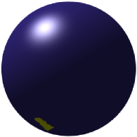
(a) DES SV

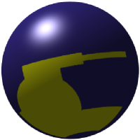
(b) DES full

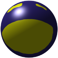
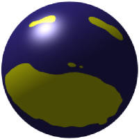
(c) Euclid (front and rear views)

Figure 1: Approximate coverage area of different weak lensing surveys illustrated on the celestial sphere. In particular, the coverage area corresponding to DES SV observations, DES full observations and Euclid observations are shown. It is apparent that existing planar mass-mapping techniques will not be appropriate for the large coverage areas of forthcoming surveys. We extend the Kaiser-Squires technique for mass-mapping to the spherical setting in this article, in order to recover mass-maps on the celestial sphere.

In this article we consider the Kaiser-Squires approach for recovering mass-maps defined on the full celestial sphere. While the harmonic space expressions in the spherical setting relating the observed shear field to the convergence field, via the lensing potential, have been presented already (e.g. Taylor, 2001; Castro et al., 2005; Pichon et al., 2010), to the best of our knowledge naive Fourier inversion on the celesital sphere (i.e. spherical Kaiser-Squires) has not been considered previously. We compare the spherical Kaiser-Squires formalism with the planar case, considering several different spherical projections. Spherical mass-mapping techniques have also been considered by Pichon et al. (2010), where a maximum a posteriori (MAP) estimator was presented. In addition, the authors consider using a Wiener filter to denoise the shear in advance of attempting to recover convergence maps. However, as far as we are aware these techniques have not been applied to observational data. The spherical Kaiser-Squires technique that we present here is a first step towards more sophisticated spherical mass-mapping techniques that will be the focus of future work. In practice only partial-fields defined on the celestial sphere are observed. The Kaiser-Squires estimator suffers due to leakage induced by the masking of the observed region (it is well-known that the decomposition of a spin field into scalar and pseudo-scalar components, and consequently mass-mapping, is not unique on a manifold with boundary; Bunn et al. 2003). Pure mode estimators on the celestial sphere can be developed to remove this leakage (e.g. Leistedt et al., 2017). Furthermore, the impact of noise can be mitigated by the use of regularisation methods adapted to the spherical setting (e.g. Wallis et al., 2016).

The remainder of this article is structured as follows. In Section 2 we briefly review the mathematical background of spin fields on the sphere and weak gravitational lensing. Mass-mapping on the celestial sphere is presented in Section 3. In Section 4 we use simulations to compare the spherical case to a variety of planar settings for various spherical projections. In Section 5 we present an application of the spherical Kaiser-Squires technique to DES SV data in order to recover spherical mass-maps. Concluding remarks are made in Section 6. Throughout we adopt the cubehelix (Green, 2011) colour scheme.

2 Background

Weak gravitational lensing gives rise to scalar and spin fields defined on the celestial sphere. For example, the observed shear field induced by weak gravitational lensing is a spin $\pm 2$ field. We therefore review scalar and spin fields on the sphere and their harmonic representation, before reviewing the mathematical details of rotation and the Dirac delta function on the sphere, which we make use of subsequently when considering mass-mapping on the celestial sphere. Weak gravitational lensing in the three-dimensional spherical setting is then reviewed concisely.

2.1 Spin fields on the sphere

Square integrable spin fields on the sphere ${}_{s}f$, with integer spin $s\in\mathbb{Z}$, are defined by their behaviour under local rotations. By definition, a spin field transforms as

$${}_{s}f^{\prime}({\omega})={\rm e}^{-{\rm i}s\chi}\>{}_{s}f({\omega})\>,$$ (1)

under a local rotation by $\chi\in[0,2\pi)$, where the prime denotes the rotated field (Newman & Penrose, 1966; Goldberg et al., 1967; Zaldarriaga & Seljak, 1997; Kamionkowski et al., 1997). It is important to note that the rotation considered here is not a global rotation on the sphere but rather a rotation by $\chi$ in the tangent plane centred on the spherical coordinates ${\omega}=(\theta,\varphi)\in{\mathbb{S}^{2}}$, with co-latitude $\theta\in[0,\pi]$ and longitude $\varphi\in[0,2\pi)$. The case $s=0$ reduces to the standard scalar setting.

The canonical basis for scalar fields defined on the sphere are given by the (scalar) spherical harmonics $Y_{\ell m}$. Basis functions for spin fields can be defined by applying spin lowering and raising operators to the scalar spherical harmonics. Spin raising and lowering operators, $\eth$ and $\bar{\eth}$ respectively, increment and decrement the spin order of a spin-$s$ field by unity and are defined by

$$\eth\equiv-\sin^{s}\theta\>\Biggl{(}\frac{\partial}{\partial\theta}+\frac{{\rm i}}{\sin\theta}\frac{\partial}{\partial\varphi}\Biggr{)}\>\sin^{-s}\theta$$ (2)

and

$$\bar{\eth}\equiv-\sin^{-s}\theta\>\Biggl{(}\frac{\partial}{\partial\theta}-\frac{{\rm i}}{\sin\theta}\frac{\partial}{\partial\varphi}\Biggr{)}\>\sin^{s}\theta\>,$$ (3)

respectively (Newman & Penrose, 1966; Goldberg et al., 1967; Zaldarriaga & Seljak, 1997; Kamionkowski et al., 1997). When applied to spherical harmonics the spin raising and lowering operators take the form:

$$\eth\>{{}_{s}Y_{\ell m}({{\omega}})}=\Bigl{[}(\ell-s)(\ell+s+1)\Bigr{]}^{1/2}\>{{}_{s+1}Y_{\ell m}({{\omega}})}$$ (4)

and

$$\bar{\eth}\>{{}_{s}Y_{\ell m}({{\omega}})}=-\Bigl{[}(\ell+s)(\ell-s+1)\Bigr{]}^{1/2}\>{{}_{s-1}Y_{\ell m}({{\omega}})}\>,$$ (5)

respectively (see, e.g., Zaldarriaga & Seljak, 1997). The spin-$s$ spherical harmonics can thus be expressed in terms of the scalar (spin-zero) harmonics through the spin raising and lowering operators by

$${{}_{s}Y_{\ell m}({{\omega}})}=\biggl{[}\frac{(\ell-s)!}{(\ell+s)!}\biggr{]}^{1/2}\eth^{s}Y_{\ell m}({{\omega}})\>,$$ (6)

for $0\leq s\leq\ell$, and by

$${{}_{s}Y_{\ell m}({{\omega}})}=(-1)^{s}\biggl{[}\frac{(\ell+s)!}{(\ell-s)!}\biggr{]}^{1/2}\bar{\eth}^{-s}Y_{\ell m}({{\omega}})\>,$$ (7)

for $-\ell\leq s\leq 0$, where $Y_{\ell m}$ denote the scalar (spin-zero) spherical harmonics.

Due to the orthogonality and completeness of the spin spherical harmonics, a spin field on the sphere can be decomposed into its harmonic representation by

$${}_{s}f({\omega})=\sum_{\ell=0}^{\infty}\sum_{m=-\ell}^{\ell}{}_{s}\hat{f}_{\ell m}\>{{}_{s}Y_{\ell m}({{\omega}})}\>.$$ (8)

The harmonic coefficients of ${}_{s}f$, denoted by ${}_{s}\hat{f}$, are given by the usual projection onto the basis functions:

$${}_{s}\hat{f}_{\ell m}=\langle{{}_{s}f},\>{{\prescript{}{s}{Y}_{\ell m}}}\rangle=\int_{\mathbb{S}^{2}}\mathrm{\,d}\Omega({\omega})\>{}_{s}f({\omega})\>{{}_{s}Y_{\ell m}^{\ast}({{\omega}})}\>,$$ (9)

where the rotation invariant measure on the sphere is given by $\mathrm{\,d}\Omega({\omega})=\sin\theta\mathrm{\,d}\theta\mathrm{\,d}\varphi$, the inner product on the sphere is denoted by $\langle{\cdot},\>{\cdot}\rangle$ and $\cdot^{\ast}$ denotes complex conjugation. In practice we consider harmonic coefficients up to a maximum degree ${\ell_{\rm max}}$, i.e. signals on the sphere band-limited at ${\ell_{\rm max}}$ with ${{}_{s}f}_{{\ell}{m}}=0$, $\forall\ell\geq{\ell_{\rm max}}$, in which case summations over $\ell$ can be truncated at ${\ell_{\rm max}}$. For notational brevity, we sometimes do not explicitly show the limits of summation where these can be inferred easily.

2.2 Rotation on the sphere

We subsequently consider the rotation of fields on the sphere, defined by application of the rotation operator $\mathcal{R}_{\mathbf{\rho}}$, where the rotation is parameterised by the Euler angles $\mathbf{\rho}=(\alpha,\beta,\gamma)\in{\mathrm{SO}(3)}$. We adopt the $zyz$ Euler convention corresponding to the rotation of a physical body in a fixed coordinate system about the $z$, $y$ and $z$ axes by $\gamma$, $\beta$ and $\alpha$, respectively. Often we consider rotations with $\gamma=0$ and adopt the shorthand notation $\mathcal{R}_{{\omega}}=\mathcal{R}_{(\varphi,\theta,0)}$.

The spin spherical harmonic functions are rotated by (e.g. McEwen et al., 2015)

$$(\mathcal{R}_{\mathbf{\rho}}\>{\prescript{}{s}{Y}_{\ell m}})({\omega})=\sum_{n=-\ell}^{\ell}D_{nm}^{\ell}(\mathbf{\rho})\>{{}_{s}Y_{\ell n}({{\omega}})}\>,$$ (10)

where $D_{nm}^{\ell}$ are the Wigner $D$-functions (Varshalovich et al., 1989), which follows from the additive property of the Wigner $D$-functions (Marinucci & Peccati, 2011).

The Wigner $D$-functions may also be related to the spin spherical harmonics by (Goldberg et al., 1967)

$${\rm e}^{-{\rm i}s\gamma}{{}_{s}Y_{\ell m}({\beta,\gamma})}=(-1)^{s}\sqrt{\frac{2\ell+1}{4\pi}}\>D_{m,-s}^{\ell\>\ast}(\alpha,\beta,\gamma)\>.$$ (11)

2.3 Dirac delta on the sphere

We subsequently make use of the Dirac delta function on the sphere $\delta^{\rm D}$, defined by

$$(\mathcal{R}_{{\omega}^{\prime}}\delta^{\rm D})({\omega}) =\frac{1}{\sin\theta}\>\delta^{1{\rm D}}(\theta-\theta^{\prime})\>\delta^{1{\rm D}}(\varphi-\varphi^{\prime})$$ (12)

$$=\sum_{\ell=0}^{\infty}\sum_{m=-\ell}^{\ell}Y_{\ell m}^{\ast}({{\omega}^{\prime}})\>Y_{\ell m}({{\omega}})\>,$$ (13)

where $\delta^{1{\rm D}}(\cdot)$ denotes the standard one-dimensional (Euclidean) Dirac delta. The spherical harmonic coefficients of the Dirac delta defined on the sphere are given by

$${\hat{\delta}}_{{\ell}{m}}^{\rm D}=Y_{\ell m}^{\ast}({\mbox{\boldmath${0}$}})=\sqrt{\frac{2\ell+1}{4\pi}}\>\delta_{{m}{0}}\>.$$ (14)

2.4 Weak gravitational lensing

We now turn our attention to weak gravitational lensing, concisely reviewing the related mathematical background, which is covered in more depth in several review articles (e.g. Bartelmann & Schneider, 2001; Schneider, 2005; Munshi et al., 2008; Heavens, 2009).

The weak gravitational lensing effect is typically expressed in terms of the lensing potential $\phi$, which depends on the integrated deflection angle along the line of sight, sourced by the local Newtonian potential $\Phi$:

$$\phi(r,{\omega})=\frac{2}{c^{2}}\int_{0}^{r}{\rm d}r^{\prime}\frac{f_{K}(r-r^{\prime})}{f_{K}(r)f_{K}(r^{\prime})}\ \Phi(r^{\prime},{\omega})\>,$$ (15)

where $c$ is the speed of light in a vacuum, $r$ and $r^{\prime}$ are comoving distances, and ${\omega}=(\theta,\varphi)$ denote spherical coordinates, as defined previously. The angular diameter distance factor reads

$$f_{K}(r)=\left\{\begin{array}[]{lll}\sin(r),&{\rm if}\ K=1\vspace*{2mm}\\ r,&{\rm if}\ K=0\vspace*{2mm}\\ \sinh(r),&{\rm if}\ K=-1\end{array}\right.\>,$$ (16)

for cosmologies with positive ($K=1$), flat ($K=0$) and negative ($K=-1$) global curvatures. This expression assumes the Born approximation. The gravitational potential is related to the density field by Poisson’s equation,

$$\nabla^{2}\Phi(r,{\omega})=\frac{3\Omega_{\rm M}H_{0}^{2}}{2a(r)}\>\delta(r,{\omega})\>,$$ (17)

where $\Omega_{\rm M}$ is the current average matter density of the Universe as a fraction of the critical density, $H_{0}$ is the current expansion rate of the Universe, $a(r)$ is the scale factor, and $\delta$ is the fractional matter over-density. Equation (15) and Equation (17) relate the matter perturbations $\delta$ to the lensing potential $\phi$.

The lensing potential describes how light from a background source (e.g. galaxy) at a position $(r,{\omega})$ is distorted by the lensing effect. This deflection, to first order, affects the images of galaxies in two ways. Firstly, images of background sources are magnified by the convergence $\kappa$, which is related to the lensing potential by

$$\prescript{}{0}{\kappa}(r,{\omega})=\tfrac{1}{4}\bigl{(}\eth\bar{\eth}+\bar{\eth}\eth\bigr{)}\prescript{}{0}{\phi}(r,{\omega})\>,$$ (18)

through the spin raising and lowering operators introduced in Equation (2) and Equation (3). The convergence is not measured directly in weak lensing experiments because the intrinsic magnitude of galaxy sizes is unknown. Here and subsequently we denote the spin of each field explicit with a proceeding subscript, i.e. $\prescript{}{0}{\phi}=\phi$ and $\prescript{}{0}{\kappa}=\kappa$ are both spin-zero (scalar) fields. Secondly, images of background sources are sheared by $\prescript{}{2}{\gamma}$, which is related to the lensing potential by

$$\prescript{}{2}{\gamma}(r,{\omega})=\tfrac{1}{2}\eth\eth\prescript{}{0}{\phi}(r,{\omega})\>,$$ (19)

where we make it explicit that the shear is a spin-2 field. Upon averaging the shapes of many galaxies one would expect the intrinsic shear to average to zero (i.e. there is no preferred orientation). Hence, one can measure shear by averaging the shapes of many galaxies. In the remainder of this article we do not consider “tomography” (the separation of a source galaxy sample into populations labelled by redshift or time) and so drop the radial dependence shown in the above equations (for notational brevity, henceforth we typically do not show the angular dependence either). For further information see the discussions in Kitching et al. (2016) on spherical-radial and spherical-Bessel representations of the shear field.

In general the potential $\prescript{}{0}{\phi}$ can be decomposed into its parity even and parity odd components, namely the E-mode and B-mode components respectively:

$$\prescript{}{0}{\phi}=\prescript{}{0}{\phi}^{\rm E}+{\rm i}\prescript{}{0}{\phi}^{\rm B}\>.$$ (20)

However, the shear induced by gravitational lensing produces an E-mode field only since density (scalar) perturbations cannot induce a parity odd B-mode component. In the absence of systematic effects, we have $\prescript{}{0}{\phi}^{\rm E}=\prescript{}{0}{\phi}$ and $\prescript{}{0}{\phi}^{\rm B}=0$. The convergence can also be decomposed into a parity even E-mode component and a parity odd B-mode component:

$$\prescript{}{0}{\kappa}=\prescript{}{0}{\kappa}^{\rm E}+{\rm i}\prescript{}{0}{\kappa}^{\rm B}\>,$$ (21)

where the B-mode component is again zero in the absence of systematics effects. While the E-mode convergence field is of most interest in the standard cosmological model, the B-mode convergence field is important for testing for residual systematics. Moreover, B-modes are also useful in studying exotic cosmological models that exhibit parity violation (e.g. Kaufman et al., 2016).  Theoretical models of intrinsic alignments of galaxies can create $B$-modes (Hirata & Seljak, 2004; Crittenden et al., 2001, 2002), although the measured level is uncertain (Kirk et al., 2015).

The E-mode convergence field represents a scaled version of the integrated mass distribution and thus mapping the intervening matter distribution is often performed by estimating the convergence field. Since the shear is related to the convergence via the lensing potential through Equation (18) and Equation (19), convergence maps can be recovered from the observable shear field, which amounts to solving an inverse problem.

3 Mass-mapping on the celestial sphere

In this section we describe the process of estimating a convergence field from an observed shear field in the spherical setting. Recovering mass-maps by estimating the convergence field involves solving a spherical inverse problem, as discussed above. First, we define the forward problem in spherical harmonic space and explicitly define the spherical generalisation of the Kaiser-Squires estimator for solving this inverse problem. Second, we present an equivalent real space representation of the spherical mass-mapping inverse problem, where it can be seen as a deconvolution problem with a spin kernel. Third, we consider the planar approximation of the full spherical setting, recovering the standard planar Kaiser-Squires estimator. Finally, we consider iterative refinements to convergence estimators that account for the fact that it is the reduced shear that is observed, rather than the true underlying shear.

3.1 Harmonic representation

Using the harmonic representations of the spin raising and lowering operators it is straightforward to show that the harmonic representations of the convergence and cosmic shear of Equation (18) and Equation (19) read, respectively,

$$\prescript{}{0}{\hat{\kappa}}_{{\ell}{m}}=-\tfrac{1}{2}\ell(\ell+1)\>\prescript{}{0}{\hat{\phi}}_{{\ell}{m}}$$ (22)

and

$$\prescript{}{2}{\hat{\gamma}}_{{\ell}{m}}=\frac{1}{2}\sqrt{\frac{(\ell+2)!}{(\ell-2)!}}\>\prescript{}{0}{\hat{\phi}}_{{\ell}{m}}\>,$$ (23)

where $\prescript{}{0}{\hat{\phi}}_{{\ell}{m}}$ and $\prescript{}{0}{\hat{\kappa}}_{{\ell}{m}}$ are the scalar spherical harmonic coefficients of the lensing potential and the converge field respectively, and $\prescript{}{2}{\hat{\gamma}}_{{\ell}{m}}$ are the spin-2 spherical harmonic coefficients of the cosmic shear field, i.e. $\prescript{}{0}{\hat{\phi}}_{{\ell}{m}}=\langle{\prescript{}{0}{\phi}},\>{Y_{\ell m}}\rangle$, $\prescript{}{0}{\hat{\kappa}}_{{\ell}{m}}=\langle{\prescript{}{0}{\kappa}},\>{Y_{\ell m}}\rangle$, and $\prescript{}{2}{\hat{\gamma}}_{{\ell}{m}}=\langle{\prescript{}{2}{\gamma}},\>{{\prescript{}{2}{Y}_{\ell m}}}\rangle$. It follows that the spin-2 harmonic coefficients of the shear are related to the scalar harmonic coefficients of the convergence by

$$\prescript{}{2}{\hat{\gamma}}_{{\ell}{m}}=\mathcal{D}_{\ell}\prescript{}{0}{\hat{\kappa}}_{{\ell}{m}}\>,$$ (24)

where we define the kernel

$$\mathcal{D}_{\ell}=\frac{-1}{\ell(\ell+1)}\sqrt{\frac{(\ell+2)!}{(\ell-2)!}}\>.$$ (25)

Recovering the convergence field from the observable shear field therefore amounts to solving the inverse problem defined by Equation (24). The simplest method to invert this problem is to consider a direct inversion in harmonic space. In the planar setting, such an approach gives rise to the Kaiser-Squires estimator (Kaiser & Squires, 1993). An analogous approach in the full-sky setting leads to the spherical generalisation of the Kaiser-Squires estimator, defined by

$${}_{0}\hat{\kappa}^{\rm SKS}_{\ell m}=\mathcal{D}_{\ell}^{-1}\prescript{}{2}{\hat{\gamma}}_{{\ell}{m}}^{\rm est}\>,$$ (26)

where $\hat{\gamma}^{\rm est}_{\ell m}$ denotes the estimate of the shear harmonic coefficients computed from observational data and ${}_{0}\hat{\kappa}^{\rm SKS}_{\ell m}$ is the spherical Kaiser-Squires (SKS) estimator of the harmonic coefficients of the convergence field. A spherical convergence map $\prescript{}{0}{\kappa}^{\rm SKS}({\omega})$ can then be recovered by an inverse scalar spherical harmonic transform, following Equation (8), from which the E- and B-mode components can be determined by considering the real and complex components, following Equation (21).

It is well-known that a direct Fourier inversion approach to solving inverse problems, on which the Kaiser-Squires estimator is based, is susceptible to noise. On large scales one typically draws a central limit theory argument for noise Gaussianity, in which case a mutlivariate Gaussian noise model is adopted. In such settings the Kaiser-Squires approach is straightforwardly given by the maximum likelihood estimator, which implicitly assumes a uninformative flat prior. This, combined with the fact that the Kaiser-Squires inversion kernel defined by Equation (24) has a flat frequency response, indicates that noise present in the observational dataset propagates unchecked into the convergence estimate.

Typically one may wish to adopt more informative priors, within a Bayesian setting, to regularise this noise contribution (see e.g. Pichon et al., 2010; Price et al., 2021, where Gaussian and wavelet sparsity priors are adopted respectively). However, for the Kaiser-Squires approach the recovered convergence field is, somewhat naively, smoothed with a Gaussian kernel to mitigate the impact of noise. In this paper we adopt this post-processing Gaussian smoothing approach and leave more advanced alternatives to future research.

3.2 Real space representation

It is insightful to express the forward problem connecting the observable cosmic shear and the convergence field in real space. The differential form of this problem is readily apparent from Equation (18) and Equation (19), from which it follows that

$$\prescript{}{2}{\gamma}=2\>\eth\eth\>\bigl{(}\eth\bar{\eth}+\bar{\eth}\eth\bigr{)}^{-1}\prescript{}{0}{\kappa}\>.$$ (27)

An integral form can also be recovered, where the real space spin-2 shear field is related to the scalar convergence by a type of spherical convolution with a spin-2 kernel $\prescript{}{2}{\mathcal{K}}$:

$$\prescript{}{2}{\gamma}({\omega})=\int_{\mathbb{S}^{2}}\mathrm{\,d}\Omega({\omega}^{\prime})\>(\mathcal{R}_{{\omega}^{\prime}}\prescript{}{2}{\mathcal{K}})({\omega})\>\prescript{}{0}{\kappa}({\omega}^{\prime})\>,$$ (28)

where the rotation operator $\mathcal{R}_{{\omega}^{\prime}}$ is defined in Section 2.2. From comparison with Equation (27) is it apparent that the kernel is given by

$$\prescript{}{2}{\mathcal{K}}({\omega})=2\>\eth\eth\>\bigl{(}\eth\bar{\eth}+\bar{\eth}\eth\bigr{)}^{-1}\>\delta^{\rm D}({\omega})\>,$$ (29)

where $\delta^{\rm D}({\omega})$ is the Dirac delta function on the sphere defined in Section 2.3. Noting the spherical harmonic representation of the Dirac delta function of Equation (14) and the harmonic action of the spin raising and lowering operators of Equation (4) and Equation (5), it is straightforward to show that the harmonic coefficients of the kernel read

$${\prescript{}{2}{\mathcal{K}}}_{{\ell}{m}}=\frac{-1}{\ell(\ell+1)}\sqrt{\frac{(\ell+2)!}{(\ell-2)!}}\sqrt{\frac{2\ell+1}{4\pi}}\>\delta_{{m}{0}}\>.$$ (30)

An explicit expression for the kernel in real space can then be recovered from its harmonic representation, yielding

$$\prescript{}{2}{\mathcal{K}}({\omega})=\sum_{\ell}\frac{-1}{\ell(\ell+1)}\frac{2\ell+1}{4\pi}\>P_{\ell}^{2}({\cos\theta})\>,$$ (31)

where $P_{\ell}^{2}({\cdot})$ is the associated Legendre function of order two. The equivalence of the harmonic and real space expressions of the forward problem of Equation (24) and Equation (28), respectively, can also be seen by the explicit harmonic representation of Equation (28), as shown in Appendix A.

3.3 Planar approximation

We now consider the planar approximation of the spherical mass-mapping estimator presented in Section 3.1, recovering the standard planar Kaiser-Squires estimator (Kaiser & Squires, 1993). Firstly, we note the planar approximations of the spin raising and lowering operators given by

$$\eth\approx-\bigl{(}\partial_{x}+{\rm i}\partial_{y}\bigr{)}$$ (32)

and

$$\bar{\eth}\approx-\bigl{(}\partial_{x}-{\rm i}\partial_{y}\bigr{)}\>,$$ (33)

respectively (see, e.g., Bunn et al., 2003). In the planar approximation the convergence and cosmic shear are then related to the lensing potential by

$$\prescript{}{0}{\kappa}=\tfrac{1}{4}\bigl{(}\eth\bar{\eth}+\bar{\eth}\eth\bigr{)}\prescript{}{0}{\phi}\approx\tfrac{1}{2}\bigl{(}\partial_{x}^{2}+\partial_{y}^{2}\bigr{)}\prescript{}{0}{\phi}$$ (34)

and

$$\prescript{}{2}{\gamma}=\tfrac{1}{2}\eth\eth\prescript{}{0}{\phi}\approx\biggl{[}\tfrac{1}{2}\bigl{(}\partial_{x}^{2}-{\rm i}\partial_{y}^{2}\bigr{)}+{\rm i}\partial_{x}\partial_{y}\biggr{]}\prescript{}{0}{\phi}\>,$$ (35)

respectively. It is common to decompose the shear component into its real and imaginary component by

$$\prescript{}{2}{\gamma}=\gamma_{1}+{\rm i}\gamma_{2}\>.$$ (36)

The planar Fourier representations of Equation (34) and Equation (35) are then given by

$$\prescript{}{0}{\hat{\kappa}(k_{x},k_{y})}=-\tfrac{1}{2}\bigl{(}k_{x}^{2}+k_{y}^{2}\bigr{)}\prescript{}{0}{\hat{\phi}(k_{x},k_{y})}$$ (37)

and

$$\begin{split}{\hat{\gamma}_{1}(k_{x},k_{y})}&=-\tfrac{1}{2}\bigl{(}k_{x}^{2}-k_{y}^{2}\bigr{)}\prescript{}{0}{\hat{\phi}}^{\rm E}(k_{x},k_{y})+k_{x}k_{y}\prescript{}{0}{\hat{\phi}}^{\rm B}(k_{x},k_{y})\>,\\ {\hat{\gamma}_{2}(k_{x},k_{y})}&=-k_{x}k_{y}\prescript{}{0}{\hat{\phi}}^{\rm E}(k_{x},k_{y})-\tfrac{1}{2}\bigl{(}k_{x}^{2}-k_{y}^{2}\bigr{)}\prescript{}{0}{\hat{\phi}}^{\rm B}(k_{x},k_{y})\>,\end{split}$$ (38)

respectively, where $\hat{\cdot}$ denotes the Fourier transform and $k_{x}$ and $k_{y}$ denote the Fourier coordinates, and we make use of the Fourier derivative property $\widehat{\partial_{x}f}={\rm i}k_{x}\hat{f}$. It follows that under the planar approximation the shear can be related to the convergence in Fourier space by

$$\prescript{}{2}{\hat{\gamma}(k_{x},k_{y})}=\mathcal{E}_{k_{x},k_{y}}\prescript{}{0}{\hat{\kappa}(k_{x},k_{y})}\>,$$ (39)

where

$$\mathcal{E}_{k_{x},k_{y}}=\frac{k_{x}^{2}-k_{y}^{2}+{\rm i}2k_{x}k_{y}}{k_{x}^{2}+k_{y}^{2}}\>.$$ (40)

Analogous to the spherical setting considered in Section 3.1, in the planar setting recovering the convergence field from the shear amounts to solving the inverse problem defined by Equation (39). Again, the simplest method to invert this problem is to perform a direct inversion in harmonic space, which gives rises to the standard planar Kaiser-Squires (KS) estimator (Kaiser & Squires, 1993) of

$${}_{0}\hat{\kappa}^{\rm KS}(k_{x},k_{y})=\mathcal{E}_{k_{x},k_{y}}^{-1}\>{}_{2}\hat{\gamma}^{\rm est}(k_{x},k_{y})=\mathcal{E}_{k_{x},k_{y}}^{\ast}\>{}_{2}\hat{\gamma}^{\rm est}(k_{x},k_{y})\>,$$ (41)

where we have taken advantage of the fact that $\mathcal{E}_{k_{x},k_{y}}^{-1}=\mathcal{E}_{k_{x},k_{y}}^{*}$ since $|\mathcal{E}_{k_{x},k_{y}}|=1$. Recall that ${}_{2}\hat{\gamma}^{\rm est}(k_{x},k_{y})$ is the estimate of the planar Fourier coefficients of the shear computed from observational data. Expanding the real and imaginary components, one recovers the familiar KS estimators for the E- and B-mode component of the convergence given by

$${}_{0}\hat{\kappa}^{\rm E,KS}(k_{x},k_{y})=\frac{(k_{x}^{2}-k_{y}^{2})\>{}_{2}\hat{\gamma}^{\rm est}_{1}(k_{x},k_{y})+2k_{x}k_{y}\>{}_{2}\hat{\gamma}^{\rm est}_{2}(k_{x},k_{y})}{k_{x}^{2}+k_{y}^{2}}$$ (42)

and

$${}_{0}\hat{\kappa}^{\rm B,KS}(k_{x},k_{y})=\frac{-2k_{x}k_{y}\>{}_{2}\hat{\gamma}^{\rm est}_{1}(k_{x},k_{y})+(k_{x}^{2}-k_{y}^{2})\>{}_{2}\hat{\gamma}^{\rm est}_{2}(k_{x},k_{y})}{k_{x}^{2}+k_{y}^{2}}\>,$$ (43)

respectively. A planar convergence map $\prescript{}{0}{\kappa}^{\rm KS}({\omega})$ can then be recovered by an inverse Fourier transform.

In the above derivation we have not considered the practicalities of the projection of the fields considered, which are defined natively on the celestial sphere, onto a planar region. In practice, one must choose a specific projection, the choice of which can have a large impact on the quality of the convergence map recovered from the observed shear. We describe a variety of projections in Appendix B and discuss their properties. Care must be taken when projecting a spin-$2$ field such as the cosmic shear as local rotations must be taken into account, as described in detail in Appendix B.

3.4 Reduced shear

In deriving the estimators presented in Section 3.1 and Section 3.3 we made the assumption that one could observe the pixelised shear field directly. However, in practice one can only measure the pixelised reduced shear ${}_{2}{g}$, which is related to the true underlying shear by

$${}_{2}{}g=\frac{{}_{2}\gamma}{1-{}_{0}\kappa}\>.$$ (44)

The problem of recovering the convergence field then becomes non-linear. However, this non-linear problem can be solved iteratively (Seitz & Schneider, 1995; Mediavilla et al., 2016, p.153), as discussed below. These techniques and similar are in common use in the literature (e.g. Jullo et al., 2014; Lanusse et al., 2016; Price et al., 2021)

The first step is to denoise the map of reduced shear. In this work we use a Gaussian smoothing. We make an initial estimate of the shear by assuming it is simply the measured reduced shear. Then an initial estimate of the pixelised convergence field is made. The first step of the iterative algorithm is thus:

$$\begin{split}{}_{2}\gamma^{(0)}&={}_{2}g\>,\\ {}_{0}\kappa^{(0)}&=\mathsf{M}\left[{}_{2}\gamma^{(0)}\right]\>,\end{split}$$ (45)

where $\mathsf{M}$ denotes the mass-mapping estimator used to recover the convergence from the shear (in this article we consider either the spherical or planar Kaiser-Squires estimators described in Section  3.1 and Section 3.3, respectively) and the superscript denotes iteration number. We then use our estimate of the convergence to update the estimate of the shear and repeat. The $(i+1)$-th iteration is thus:

$$\begin{split}{}_{2}\gamma^{(i+1)}&={}_{2}g(1-{}_{0}\kappa^{(i)})\>,\\ {}_{0}\kappa^{(i+1)}&=\mathsf{M}\left[{}_{2}\gamma^{(i+1)}\right]\>.\end{split}$$ (46)

Iterations are continued until the absolute difference of the convergence between iterations is below some threshold value. In this work we choose,

$$\max_{j}\>\bigl{|}{}_{0}\kappa_{j}^{(i)}-{}_{0}\kappa_{j}^{(i-1)}\bigr{|}<10^{-10},$$ (47)

where $j$ runs over all pixels. Typically, for a convergence field including ellipticity/shot noise, $4$ to $5$ iterations are required before converging.

3.5 Implementation

We have written the python package massmappy to implement the algorithms presented. The package can perform standard mass-mapping on the plane, with the option to perform iterations to account for reduced shear. We also implement the spherical Kaiser-Squires estimator described above so that mass-mapping can be performed on the celestial sphere. We support the use of two spherical pixelisations schemes. Firstly, we support the use of HEALPix (Górski et al., 2005), an equal area pixelisation with an accompanying software package that can perform fast spherical harmonic transforms. We also support the use of the standard equiangular sampling scheme implemented in SSHT (McEwen & Wiaux, 2011). This sampling scheme supports fast spherical harmonic transforms that are theoretically exact and achieve close to floating point precision in practice. The most recent release of SSHT includes fast routines to compute the projections of the sphere onto the plane considered in this work.

4 Evaluation on simulations

In this section we evaluate the mass-mapping algorithms presented in Section 3 on simulations. We study the error introduced by the planar approximation, for a variety of projections and for varying survey coverage area, when compared to the spherical setting. We also assess the ability of the iterative algorithm described in Section 3.4 to deal with the reduced shear that is observed, rather than the underlying true shear.

4.1 Comparison of planar and spherical mass-mapping

We study the impact of the flat-sky planar approximation in mass-mapping, compared to the spherical setting, and determine the typical errors induced for the sky coverages of upcoming surveys. We do this as an idealised situation to focus the study on the effect of projecting the sphere on to the plane. To do so we need to understand how best one can estimate mass-maps on the plane for large coverage areas.

When creating convergence maps on the plane (i.e. mass-maps), the exact projection used to map the celestial sphere to the plane can have a large impact on the quality of the reconstructed convergence map. In Appendix B we describe a variety of spherical projections that can be considered, which we evaluate on simulations here. One important aspect when projecting a non-zero spin field, e.g. shear (or galaxy ellipticities), is to ensure that the correct local rotations are performed, as described in Appendix B.2. This is typically neglected in existing mass-mapping works.

Cylindrical
Mercator
Sinusoidal
	(a) $\gamma_{1}$	(b) $\gamma_{2}$	(c) $\kappa^{\rm E,KS}$	(d) $\kappa^{\rm E,KS}$ error	(e) $\kappa^{\rm B,KS}$ error

Figure 2: Simulated reconstructions of the convergence field (mass-maps) on large regions of the celestial sphere when using equatorial projections, in order to assess the impact of different planar projections. The shear field is shown in the first and second columns (the first showing $\gamma_{1}$ and the second showing $\gamma_{2}$). The third column shows the reconstructed convergence field ($E$-mode), while the forth and fifth columns shows the error on the $E$-mode and $B$-mode convergence, respectively. Each row shows a different projection: the first row shows the simple cylindrical projection; the second shows the Mercator projection; and the final row shows the sinusoidal projection. The entire sphere is projected onto the plane, except for the Mercator projection where only $7\pi/16$ radians above and below the equator are considered (as explained in the main text).

Orthographic
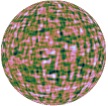
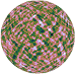
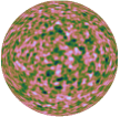
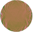
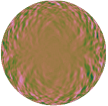
Stereographic
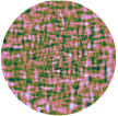
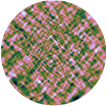
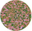
Gnomonic
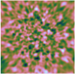
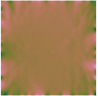
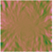
	(a) $\gamma_{1}$	(b) $\gamma_{2}$	(c) $\kappa^{\rm E,KS}$	(d) $\kappa^{\rm E,KS}$ error	(e) $\kappa^{\rm B,KS}$ error

Figure 3: Same as Fig. 2 for the polar projections. The first row shows the orthographic projection, the middle row shows the stereographic projection, and the third row shows the Gnomonic projection. For these projections we only project one hemisphere onto the sphere, with the pole defined by the $x$-axis. The entire hemisphere is shown except for the Gnomonic projection where we project the sphere onto a square where distance from the centre of the square and the edge represents an angle of $\pi/4$ radians (as explained in the main text). Of course, planar approaches are typically restricted to a field of view of $\sim 20$ degrees, these figures simply illustrate why this consensus is adhered to.

We now describe the simulations that we use to assess the effect each projection has on the quality of the reconstruction of convergence maps. We simulate Gaussian convergence maps using a convergence power spectrum generated by the software package cosmosis (Zuntz et al., 2015). The power spectrum was generated with a standard $\Lambda$CDM cosmology with galaxies in high redshift bin $z\gtrsim 1$. We simulate the map up to a harmonic band-limit of ${\ell_{\rm max}}=512$ using the sampling of the sphere of SSHT (McEwen & Wiaux, 2011). We consider this spherical sampling scheme for these numerical experiments since the resulting spherical harmonic transforms are theoretically exact and the implementations in SSHT achieve accuracy close to machine precision (which is not the case for HEALPix; see Leistedt et al. (2013) for concise accuracy benchmarks). Any errors will therefore be due to projection effects rather than inaccuracies in harmonic transforms. We smooth the simulated convergence maps with the Gaussian kernel $G_{\ell}=e^{-\ell^{2}\sigma^{2}}$, with $\sigma=\pi/256$, to mitigate pixelisation issues. The shear field is simulated by transforming the scalar convergence field to harmonic space and then applying Equation (24), before transforming back to real space to recover a spin-2 shear field on the celestial sphere. In these simulations we aim to understand the effect of the projections so we do not consider the effects of reduced shear or noise.

To evaluate the accuracy of planar mass-mapping we first project the simulated shear field from the celestial sphere to the plane, using a particular projection. We estimate the convergence field from the planar shear field using the planar KS estimator of Equation (41). We then compare this recovered planar convergence to a planar projection of the convergence simulated initially on the celestial sphere. A number of different projections are considered, as defined in Appendix B. In general, we consider two classes of spherical projection: namely, equatorial and polar projections.

In Fig. 2 we show example planar reconstructions and errors for a variety of equatorial projections. These projections are highly accurate on the equator, with distortion due to the projection typically increasing with distance from the equator. We consider, firstly, a simple cylindrical projection, where the $(\theta,\varphi)$ angles are taken to be Cartesian coordinates $(x,y)$. We also consider the Mercator projection, which is often used for geographical maps. The Mercator projection is a conformal projection, in that it preserves local angles. The poles in this projection would be at infinity, so we limit the projection to $7\pi/16$ radians above and below the equator. Finally, Fig. 2 shows results using the sinusoidal projection, a simple equal area projection used by the DES collaboration for the convergence map generated from DES SV data (Vikram et al., 2015).

In Fig. 3 we show example planar reconstructions and errors for a variety of polar projections. These projections are highly accurate around the pole defining the centre of the projection, with distortion increasing as one moves away from this point. For these projections we project one hemisphere around a pole defined by the $x$-axis only; hence, two projections (one for each hemisphere) are required to cover the entire sphere. We consider the orthographic projection, which is a simple vertical projection, the stereographic projection, which is another conformal projection, and finally the Gnomonic projection, which has the special property that the local rotations required for the projection of spin fields are zero (if no coordinate rotation is performed). The edge of the hemisphere for the Gnomonic projection lies at infinity so we only project the sphere onto the square where the distance from the centre of the square and its edge represents an angle of $\pi/4$ radians.

For all projections, we show in Fig. 2 and Fig. 3 the projected shear, the recovered $E$-mode convergence and the error in the $E$ and $B$-mode convergence. As expected the convergence reconstruction is best where the planar approximation is most accurate and worse as one moves away from this region. We can also see by eye that the conformal projections (the Mercator and stereographic projections) perform the best. This is due to fact that local angles are preserved by the projection. What is also clear is that for many of the projections the $B$-mode convergence error can be large in certain regions even in the absence of noise or systematic errors.

(a) $\kappa^{\rm KS}$ $E$-mode error

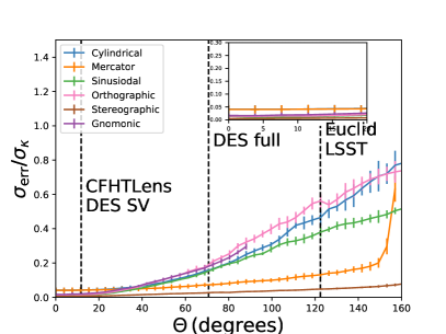
(b) $\kappa^{\rm KS}$ $B$-mode error

Figure 4: Relative RMS error of recovered convergence fields (mass-maps) when using various planar projections in the standard planar Kaiser-Squires (KS) estimator, as a function of angular distance from the centre of the projection. Note that all planar projections were significantly zero-padded (to 4 times their original dimension) to minimise any contribution to this error from mode mixing at boundaries. Further we note that residual boundary effects inevitably exist, thus we clip the figure 20 degrees from any boundary, thus restricting the figure to $\Theta$ domains over which it is expected the primary error contribution comes from projection effects. RMS errors are averaged over 10 realisations. Approximate opening angles for the coverages of existing and upcoming surveys are overlaid. For future surveys, such as Euclid and LSST, projection errors can be of order tens of percent, exceeding 50% in some cases. The conformal projections (i.e. the Mercator and stereographic projections), which preserve local angles, are typically superior to the other projections. In any case, these errors can be avoided entirely by recovering convergence fields directly on the celestial sphere.

We can use these simulations to examine the error in the reconstructed convergence field as a function of angular size. In Fig. 4 we show how the accuracy of the recovered convergence field changes with patch size. We consider a similar simulation setup as the low resolution experiments described above but now simulate the convergence field up to a band limit ${\ell_{\rm max}}=4000$, using the same power spectrum and smoothing kernel as before. We set a higher band-limit to eliminate all pixelisation effects (a lower band-limit was sufficient for the previous numerical experiments which were used for visualisation purposes only). We over-sample on the plane too, again to eliminate all pixelisation effects. For the polar projections we use a square map of $2000\times 2000$ pixels, capturing the same hemisphere as before. For the equatorial projections we use maps of size $(2{\ell_{\rm max}}-1)\times{\ell_{\rm max}}$ pixels for the cylindrical projection, $(2{\ell_{\rm max}}-1)\times 5901$ pixels for the Mercator projection and $(2{\ell_{\rm max}}-1)\times{\ell_{\rm max}}$ pixels for the sinusoidal projection. The number of pixels is different of the Mercator projection as it stretches the $\theta$ direction in projection. The equatorial projections, as before, have the entire sphere projected onto the plane except for the Mercator projection where we project to $7\pi/16$ radians above and below the equator only as the poles are at infinity in this projection. The exact planar sampling resolutions are not important as we are intentionally over-sampling to eliminate pixelisation effects.

In a similar way to the other simulations we simulate the convergence and shear on the sphere, project the shear on the plane, and recover the convergence on the plane to compare this to the projected simulated convergence. We then calculate the root-mean-square (RMS) error of $\frac{1}{N}\sum_{i}^{N}(\kappa^{\rm KS}-\kappa^{\rm input})^{2}$ at different angular distances from the most accurate region of each projection, where $N$ is the number of pixels in the region and $\kappa^{\rm input}$ is the input convergence. The exact angular distances considered for each projection are defined in Appendix B. We calculate the error in annuli of constant angular distances away from the centre, defined by the angular metric. The error in the recovered convergence will be a result of not only the projection distortion but also a sub-dominant contribution from the leakage due to the boundary created by the projection. The leakage due to boundary effects will be minimal for small and intermediate scales but will become more significant for the largest scales considered – i.e. as the annuli approach the boundary region. Both projection and boundary effects are intrinsic to the projection when using KS inversion and are therefore included here. To minimise the contribution of such boundary effects we zero-pad planar projections to 4 times their original dimensions, and restrict any analysis to annuli separated by at least 20 degrees from any boundaries.

Fig. 4 shows the RMS error, averaged over 10 realisations, at different angular distances for the various projections considered. We normalise the RMS error with the RMS of the fluctuations in that region to give a relative error. Relative error for both the $E$- and $B$-modes fields are shown. Approximate opening angles for the coverages of existing and upcoming surveys are overlaid on Fig. 4. For future surveys, such as Euclid and LSST, projection errors can be of order tens of percent, exceeding 50% in some cases. The conformal projections (i.e. the Mercator and stereographic projections), which preserve local angles, are typically superior to the other projections. In any case, these errors can be avoided entirely by recovering convergence fields directly on the celestial sphere.

5 Application to DES SV data

In this section we apply the mass-mapping techniques presented in Section 3 to the DES science verification (SV) data, which are publicly available. We use the galaxy shapes estimated by the im3shape method that lie in the range $60^{{}^{\circ}}<{\rm RA}<95^{{}^{\circ}}$ and $-70^{{}^{\circ}}<{\rm dec}<-40^{{}^{\circ}}$, where ${\rm RA}$ and ${\rm dec}$ are the right ascension and declination in degrees. We apply the ${\rm\tt sva1\_flag}=0$ selection to the DES SV catalog in order to select galaxies that have a shape that is measured and calibrated ready to be used for weak lensing studies. These cuts leave $793,743$ galaxies, with a density of 1.4 galaxies per square arcmin. We pixelise the data by binning into pixels in various settings. We always pixelise the galaxy in the space that the convergence map is generated; for example, when a map is made on the sphere the galaxies are pixelated on the sphere directly. In all cases we apply the recommended weights and corrections to account for multiplicative and additive biases, as described by Becker et al. (2016).

We create two spherical maps of the reduced shear using the SSHT and HEALPix sampling schemes, considering resolutions to best match the $\delta\theta=5$ arcmin pixels considered by Vikram et al. (2015), which corresponds to setting an appropriate bandlimit ${\ell_{\rm max}}$ for the SSHT sampling scheme and an appropriate ${N_{\rm{side}}}$ resolution parameter for HEALPix. Explicitly, for SSHT, we find ${\ell_{\rm max}}=\pi/\delta\theta=2160$. For HEALPix, we set $N_{\rm side}$ such that the area of a pixel is as close as possible to that of a 5 arcmin pixel, i.e. $A=4\pi/12N_{\rm side}^{2}\approx(\delta\theta)^{2}$, yielding $N_{\rm side}=512$ (with the restriction that ${N_{\rm{side}}}$ is a power of two). The resulting SSHT map has pixels of size 5 arcmin at the equator, while the resulting HEALPix map has pixels of size $7$ arcmin. For the HEALPix sampled data we use a maximum multipole $\ell_{\rm max}=4N_{\rm side}$. The exact choice of $\ell_{\rm max}$ is not critical as smoothing removes the power on small scales. We smooth the reduced shear before reconstructing the mass-map with a Gaussian Kernel $G_{\ell}=e^{-\ell^{2}\sigma^{2}}$, with $\sigma$ such that the half width at half maxima is 20 arcmin, to best match that of Vikram et al. (2015).

It is academic to note that interpolation errors are effectively unavoidable when mapping observations continuous in position onto a finite grid. Furthermore, gridding onto different sampling schemes inherently introduces different interpolation error. One may wonder, quite reasonably, which sampling (or corrective measure) minimizes this interpolation error, however this is beyond the scope of this paper. To normalise for this effect within this analysis we first grid onto HEALPix map which we then convert into a SSHT sampled map with the aforementioned dimensions. In this way both maps begin with the same information contaminated with the same interpolation error.

Further one should note that the noise properties of interpolated spherical maps depend fundamentally on the sampling scheme adopted. When one considers HEALPix equal area sampling each pixel contains roughly the same number of observations, whereas for SSHT equiangular sampling pixels have significant variation in the number of observations (due to variability in pixel size). As such, the assumption of noise Gaussianity is more easily justified for HEALPix maps.

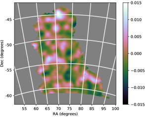
(a) $\kappa^{\rm SKS}$ $E$-mode (SSHT)

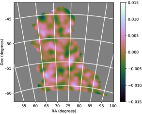
(b) $\kappa^{\rm SKS}$ $B$-mode (SSHT)

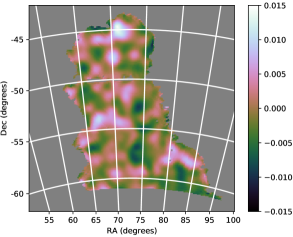
(c) $\kappa^{\rm SKS}$ $E$-mode (HEALPix)

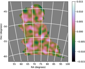
(d) $\kappa^{\rm SKS}$ $B$-mode (HEALPix)

Figure 5: Spherical convergence maps recovered by the spherical Kaiser-Squires (SKS) estimator applied to spherical maps of the reduced shear created using galaxies from DES SV data. The top two plots show stereographic projections of the convergence map recovered on the celestial sphere using the SSHT sampling, while the bottom two plots show Stereographic projections of the convergence maps recovered on the celestial sphere using HEALPix sampling. The left column shows the recovered $E$-mode convergence, while the right shows the recovered $B$-mode convergence. To generate these maps from the DES observation catalogue we first grid onto a HEALPix sampling scheme, then convert this to a SSHT sampling scheme through harmonic space, thus both reconstructions are working with the same information which mitigates any discrepancies due to the initial catalogue projection.

Fig. 5 shows the $E$- and $B$-mode convergence maps recovered from the DES SV data using the spherical Kaiser-Squires (SKS) estimators. We apply the iterative algorithm described in Section 3.4 to estimate the underlying shear from the observed reduced shear. The recovered convergence maps show near perfect agreement with each other and reasonable agreement with the maps recovered by the DES collaboration for a similar choice of galaxies (Vikram et al., 2015, Fig. 2). It should be noted that the galaxies used here are not the exact same galaxies used in estimating the convergence maps recovered by Vikram et al. (2015) due to small differences between the private and public DES catalogs (C. Chang & J. Zuntz, private communication). Therefore, exact equivalence is not excepted, however, through private communication C. Chang has provided convergence maps recovered by the DES map making pipeline when using the public catalog and in this case there is good agreement between the two convergence maps.

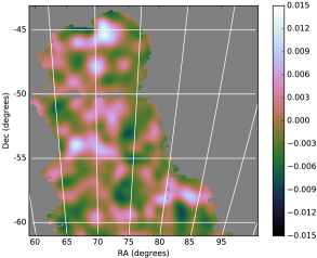
(a) $\kappa^{\rm KS}$ $E$-mode for sinusoidal projection

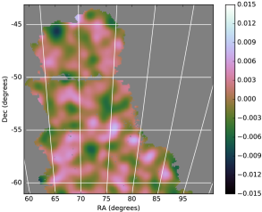
(b) $\kappa^{\rm KS}$ $B$-mode for sinusoidal projection

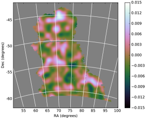
(c) $\kappa^{\rm KS}$ $E$-mode for stereographic projection

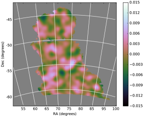
(d) $\kappa^{\rm KS}$ $B$-mode for stereographic projection

Figure 6: Planar convergence maps recovered by the planar Kaiser-Squires (KS) estimator applied to planar maps of the reduced shear created using galaxies from the DES SV data. The top row of plots show the results where the sinusoidal projection is used, while the bottom row shows the results when the stereographic projection is used. These projections were chosen since the the sinusoidal projection is used by the DES collaboration (Vikram et al., 2015), while the stereographic projection was shown in Fig. 4 to minimise RMS error. The left column shows the recovered $E$-mode convergence, while the right shows the recovered $B$-mode convergence.

For comparison purposes, in Fig. 6 we show the results when we bin galaxies onto two planar maps. The top row show the results when using a sinusoidal projection, as also used by the DES collaboration (Vikram et al., 2015). We rotate the projection such that the central line of the projection corresponds to ${\rm RA}=70^{{}^{\circ}}$, as also done by Vikram et al. (2015). No other rotation is applied to fully centre the region of interest. In the second row we show results using a stereographic projection that has been rotated by the Euler angles $\alpha=159^{{}^{\circ}}$, $\beta=-37^{{}^{\circ}}$ and $\gamma=90^{{}^{\circ}}$, to fully centre the area of interest to the South pole about which the projection is then performed. We choose to also show results using the stereographic projection as the results from Fig. 4 suggest that this is the best projection to use. In both cases we use 5 arcmin pixels and apply a 20 arcmin smoothing as they do in Vikram et al. (2015). We apply the required local rotations as described in Appendix B (in Appendix B we also examine the effect of not applying such rotations). For these planar results we also use the reduced shear algorithm described in Section 3.4. Fig. 7 shows the difference between the convergence recovered on the plane for these projections and the projected convergence recovered on the sphere using the SSHT sampling shown in Fig. 5. As is common with the KS estimator, both the planar and the spherical mass-maps suffer from leakage between the $E$- and $B$-mode due to both the effects of the boundary and, perhaps primarily, the significant complex noise contribution.

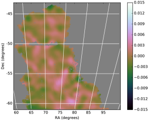
(a) $\kappa^{\rm KS}-\kappa^{\rm SKS}$ $E$-mode for sinusoidal projection

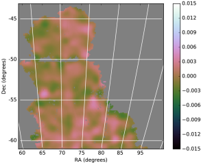
(b) $\kappa^{\rm KS}-\kappa^{\rm SKS}$ $B$-mode for sinusoidal projection

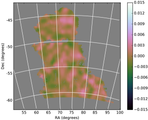
(c) $\kappa^{\rm KS}-\kappa^{\rm SKS}$ $E$-mode for stereographic projection

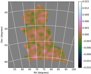
(d) $\kappa^{\rm KS}-\kappa^{\rm SKS}$ $B$-mode for stereographic projection

Figure 7: Similar to Fig. 6, where here we plot the difference between the convergence recovered on the plane by the planar Kaiser-Squires (KS) estimator and the convergence recovered on the sphere by the spherical Kaiser-Squires (SKS) estimator. The purpose of this figure is to compare the planar and spherical results. For the spherical case we consider the SSHT sampling only, i.e. differences are relative to Fig. 5(a) and Fig. 5(b).

6 Conclusions

We have described how one can recover convergence fields, or mass-maps, directly on the celestial sphere, adopting the spherical equivalent of Kaiser-Squires inversion. We demonstrate that the spherical formulation reduces to the usual flat-sky Kaiser-Squires approach in the planar approximation. We study the accuracy of the planar approximation for mass-mapping and address the important question of whether one needs to recover the convergence field on the sphere for forthcoming surveys or whether recovery on the plane would be sufficient. The comparison between the planar and spherical settings depends largely on the projection used. In Appendix B we describe a number of projections that are used in this work and show how to account for the local rotations required when projecting spin fields, such as shear, onto the plane. In Fig. 4 the relative error introduced by the planar approximation, for a variety of projections, is presented. Conformal projections, for which local angles are conserved, are found to be the most effective. Nevertheless, errors in the planar setting are typically tens of percent and can exceed 50% in some cases. These projection errors can be entirely eliminated by recovering mass-maps directly on the celestial sphere by the spherical Kaiser-Squires technique presented in this article.

We apply the spherical Kaiser-Squires estimator to the publicly available DES SV data. We present maps of the convergence field recovered on the celestial sphere using both the SSHT and HEALPix sampling schemes (see Fig. 5), accounting for the fact that one measures reduced shear, rather than the true underlying shear, by applying the iterative algorithm discussed above. We compare the results to those recovered on the plane, using the sinusoidal projection adopted by the DES collaboration and also the stereographic projection since it was found to be most effective projection for mass-mapping, particularly for large scales (see Fig. 4). In this setting we demonstrate reasonable agreement between the spherical and planar reconstructions. While the coverage area of DES SV data is not sufficiently large for the planar approximation to induce significant errors (see Fig. 4), recovering spherical mass-maps for DES SV data is nevertheless a useful demonstration of the spherical Kaiser-Squires estimator on real observational data.

In this article we consider the most naive estimator of the convergence field on the celestial sphere, namely a direct spherical harmonic inversion of the equations relating the observed shear field to the underlying convergence field, i.e. the generalisation of the Kaiser-Squires estimator from the plane to the sphere. In practice, the shear field is not observed over the entire celestial sphere, which induces leakage in the recovered convergence field for the simple harmonic estimator considered. In future work we will apply the pure mode wavelet estimators developed by Leistedt et al. (2017) to remove leakage when recovering spherical mass-maps. In addition, in future work we also intend to develop methods to better mitigate the impact of noise and to estimate the statistical uncertainties associated with recovered mass-maps (see e.g. Price et al., 2020). In all of these extensions, however, it is clear that for future surveys like Euclid and LSST it will be essential to recover mass-maps on the celestial sphere, to avoid the significant errors than are otherwise induced by planar approximations.

7 Data Availability

All data, both observational and simulated, utilized throughout this paper is publicly available and can be found alongside the open-source code-base massmappy developed during this work.

Appendix A Equivalence of different representations of spherical mass-mapping inverse problem

The equivalence of the harmonic and integral expressions, Equation (24) and Equation (28) respectively, connecting the observable cosmic shear field to the convergence field can also be shown by considering the harmonic representation of the integral expression. Consider the integral representation, decomposing the kernel and convergence field into their harmonic expansions:

$$\prescript{}{2}{\gamma}({\omega}) =\int_{\mathbb{S}^{2}}\mathrm{\,d}\Omega({\omega}^{\prime})\>(\mathcal{R}_{{\omega}^{\prime}}\prescript{}{2}{\mathcal{K}})({\omega})\>\prescript{}{0}{\kappa}({\omega}^{\prime})$$ (48)

$$=\int_{\mathbb{S}^{2}}\mathrm{\,d}\Omega({\omega}^{\prime})\>\sum_{\ell m}{\prescript{}{2}{\mathcal{K}}}_{{\ell}{m}}\>\bigl{(}\mathcal{R}_{{\omega}^{\prime}}{\prescript{}{2}{Y}_{\ell m}}\bigr{)}({\omega})\>\sum_{\ell^{\prime}m^{\prime}}\prescript{}{0}{\hat{\kappa}}_{{\ell^{\prime}}{m^{\prime}}}\>{{}_{0}Y_{\ell^{\prime}m^{\prime}}({{\omega}^{\prime}})}\>.$$ (49)

The rotation of the spin spherical harmonic in the above expression is given by

$$\bigl{(}\mathcal{R}_{{\omega}^{\prime}}{\prescript{}{2}{Y}_{\ell 0}}\bigr{)}({\omega}) =\sum_{n}D_{n0}^{\ell}({\omega}^{\prime})\>{\prescript{}{2}{Y}_{\ell n}}({\omega})$$ (50)

$$=\sqrt{\frac{4\pi}{2\ell+1}}\sum_{n}{\prescript{}{0}{Y}_{\ell n}^{\ast}}({\omega}^{\prime})\>{\prescript{}{2}{Y}_{\ell n}}({\omega})\>,$$ (51)

where it is necessary to only consider $m=0$ due to the Kronecker delta term $\delta_{{m}{0}}$ appearing in ${\prescript{}{2}{\mathcal{K}}}_{{\ell}{m}}$, as shown in Equation (30), and noting Equation (10) and Equation (11). Equation (49) can then be written as

$$\prescript{}{2}{\gamma}({\omega}) =\sum_{\ell n}\frac{-1}{\ell(\ell+1)}\sqrt{\frac{(\ell+2)!}{(\ell-2)!}}\>\prescript{}{0}{\hat{\kappa}}_{{\ell}{n}}\>{\prescript{}{2}{Y}_{\ell n}}({\omega})\>,$$ (52)

where we have noted the orthogonality of the spherical harmonics, i.e. $\langle{Y_{\ell m}},\>{Y_{\ell^{\prime}m^{\prime}}}\rangle=\delta_{{\ell}{\ell^{\prime}}}\delta_{{m}{m^{\prime}}}$. The resulting harmonic representation of Equation (28) is thus identical to Equation (24), as expected.

Appendix B Projections

In this appendix we outline the details of each projection considered. We firstly define each projection and describe its properties. Each projection has different beneficial properties, for example whether the projection is equal-area, has appropriate boundary conditions or conformal. Conformal projections conserve local angles and are often used for geographical maps. We also describe the distance metric we use for each projection to define the opening angle of the patch of sky seen by an experiment, i.e. the angle considered in Fig. 4. We then detail how to calculate the local rotation angles required when projecting spin fields, such as shear (without this rotation $E$- and $B$-modes will be misinterpreted) and finally illustrate the impact of neglecting this local rotation on DES SV data.

B.1 Projection definitions

We consider two general types of projection: equatorial and polar projections. Equatorial projections are defined relative to the equator, while polar projections are defined relative to a pole. The precise definitions of the different equatorial and polar projections are given in the following subsections. The equatorial projections considered include: the sinusoidal projection, which is a simple equal area projection that was used by the DES collaboration; the Mercator projection that is a conformal projection, often used in geographical maps as it preserves local angles; and a simple cylindrical projection. The polar projections considered include: the orthographic projection, which is a simple vertical projection from the sphere to a tangent plane; the Gnomonic projection that has the useful property that the local rotations are trivial to calculate; and the stereographic projection that is another conformal projection.

B.1.1 Equatorial projections

Figure 8: Diagram to describe graphically the equatorial projections, including the sinusoidal, Mercator and the simple cylindrical projections. These can all be seen as types of cylindrical projections since the sphere is projected onto a cylinder wrapped round the sphere. The $u$ variable simply describes how far round the cylinder a point is and is therefore give by $\phi$ (up to some arbitrary shift), except in the sinusoidal case where the $u$ variable is contracted away from the equator to ensure the projection is equal-area. The $v$ variable can vary between projections and can be specified by various functions $d(\theta)$. In the Mercator projection this function is chosen to ensure the projection is conformal. In the sinusoidal and simple cylindrical projections this function is simply $d(\theta)=\beta=\pi/2-\theta$.

Fig. 8 shows graphically how the equatorial projections can be viewed as a projection onto a cylinder wrapped round the sphere. Each projection is defined by the relation between the spherical coordinates $(\theta,\phi)$ and the planar coordinates $(u,v)$.

The sinusoidal projection (used by the DES collaboration) is defined by

$$\begin{split}u&=(\phi-\pi)\sin(\theta)\>,\\ v&=\theta.\end{split}$$ (53)

This projection results in minimal distortion in the central region $(\theta=\pi/2$, $\phi=\pi)$. Moving away from this point in any direction increases the distortion but particularly in a diagonal direction (specifically along the lines $y=x$ or $y=-x$). We define the distance metric for this projection by

$$\Theta=\sqrt{(\theta-\pi/2)^{2}+(\phi-\pi)^{2}}\>.$$ (54)

The sinusoidal projection has the useful property of being equal-area. It is simpler to define than the Mollweide projection, also an equal-area projection, which is commonly used for plotting in the cosmological community.

The Mercator projection is commonly used for geographical maps and is defined by

$$\begin{split}u&=\phi-\pi\>,\\ v&=\ln\left[\tan(\pi/2-\theta/2)\right]\>.\end{split}$$ (55)

This projection has the useful property of being conformal, meaning that local angles on the sphere will not be distorted. The projection introduces minimal distortion at the equator, while the projected image is stretched and distorted as one moves towards the pole. Since the poles themselves are at infinity the projection cannot completely cover the full sky in practice. The projection is a cylindrical projection and therefore has the correct boundary conditions in the $u$ direction. The metric used to define the angular distance from the undistorted region is simply given by

$$\Theta=|\theta-\pi/2|\>.$$ (56)

The final equatorial projection we consider is the simple cylindrical projection defined by

$$\begin{split}u&=\phi-\pi\>,\\ v&=\theta-\pi/2\>.\end{split}$$ (57)

There are no particular properties to inspire us to propose this projection over the more sophisticated cylindrical projection of the Mercator projection. Its attractiveness is in its simplicity and the ability to map the entire sphere on one plane. The distortions increase away from the equator leading to the same distance metric as the Mercator projection, i.e. Equation (56).

B.1.2 Polar projections

Figure 9: Diagram to describe graphically the polar projections, including the orthographic, stereographic and gnomic projections. In these projections a point on the sphere is projected to the tangent plane at a pole (here chosen to be the South pole). For projections around the North or South pole the angle $\phi$ is simply taken as the polar coordinate $\varphi$ in the planar space. The radial coordinate $\varrho$ is a function of the angle between the point and the pole whos tangent plane is considered ($\pi-\theta$ for the South pole). The orthographic projection is a vertical projection, giving $\varrho=\sin(\pi-\theta)$ for the tangent plane at the South pole. The gnomic projection casts a ray from the origin to the point on the sphere and through to the tangent plane, giving $\varrho=\tan(\pi-\theta)$ for the tangent plane at the South pole. Finally, the stereographic projection casts a ray from the opposite pole to the point on the sphere and through to the tangent plane, giving $\varrho=2\tan[(\pi-\theta)/2]$ for the tangent plane at the South pole. In the diagram, the point P is projected to PO, PS, and PG by the orthographic, stereographic and gnomic projections, respectively.

Fig. 9 shows a graphical representation of the polar projections, where again the spherical coordinates $(\theta,\phi)$ are projected onto the planar coordinates $(u,v)$. It is most straightforward to define these projections using polar coordinates on the plane $(\varrho,\varphi)$, which are related to the Cartesian coordinates by

$$\begin{split}u&=\varrho\cos(\varphi)\>,\\ v&=\varrho\sin(\varphi)\>.\end{split}$$ (58)

In each of the polar projections we simply have that $\varphi=\phi$. The projections differ in the way $\theta$ is mapped to $\varrho$, where each projection has its own mapping function $f$, i.e.

$$\varrho=f(\theta)\>.$$ (59)

It is a common feature of these projections that the entire sphere cannot be projected to a single plane in practice (since in many cases the opposite pole is mapped to the point at infinity). In that case we often project around the South pole as well as the North pole and consider $\varrho=f(\pi-\theta)$. We define the distance metric for these projections to be

$$\Theta=\theta\>.$$ (60)

The orthographic projection is defined by

$$\varrho=\sin(\theta)\>.$$ (61)

For this projection a point on the sphere is mapped vertically from the sphere to the tangent plane at the North pole. As a result the whole sphere cannot be projected onto one plane in practice and one must project each hemisphere onto a different plane.

We also consider the Gnomonic projection defined by casting a ray from the centre of the sphere to the point considered and then though to the tangent plane at the North pole. The Gnomonic projection is therefore defined by

$$\varrho=\tan(\theta)\>.$$ (62)

For this projection the whole sphere again cannot be projected onto one plane in practice since the equator is projected to infinity. One must again project the sphere into a number of regions, for example considering each hemisphere separately.

The final projection we consider is the stereographic projection. This is defined by casting a ray from the South pole to the point considered on the sphere and then through to the tangent plane at the North pole. The resulting projection is defined by

$$\varrho=2\tan(\theta/2)\>.$$ (63)

We can project almost all of the sphere with this projection, except near the South pole, as the South pole is mapped to infinity. This projection is conformal, preserving local angles.

B.2 Rotation angles

Spin fields on the sphere have local directions defined relative to the North pole, whereas on the plane the spin fields have their spin defined relative to some universal direction (usually the “top” of the planar map). We define this direction on the plane by ${\hat{v}}$, the unit vector in the $v$ direction. On projection, the spin field must be rotated from its original coordinate frame on the sphere to the new coordinate frame on the plane. Here we describe how to calculate this local rotation angle.

When we project from the sphere to the plane it is common to rotate our coordinate system before we project. This is done in order to centre the region of interest so that distortions due to the projection are minimised at this point. We therefore need to define a number of coordinate systems, including the original sphere, the rotated sphere and the plane. Firstly, consider a field defined on the original sphere with spherical coordinates $(\theta^{\prime},\phi^{\prime})$ and corresponding Cartesian coordinates $(x^{\prime},y^{\prime},z^{\prime})$. Consider then the rotated field, where the spherical coordinates of the rotated sphere are $(\theta,\phi)$, with corresponding Cartesian coordinates $(x,y,z)$. We define the rotation relating the primed frame to the unprimed frame by $\mathcal{R}_{\mathbf{\rho}}$, with corresponding 3D rotation matrix $\boldsymbol{\mathsf{R}}$. From the rotated sphere the field is then projected onto the plane defined by Cartesian coordinates $(u,v)$ and polar coordinates $(\varrho,\varphi)$.

We need to find the angle between ${\hat{v}}$ and the projected direction of the North pole of the original sphere. To do this we consider an infinitesimal step North on the sphere and then find the infinitesimal step this makes on the plane $(\mathrm{\,d}u,\mathrm{\,d}v)$. The rotation angle $\psi$ required is then the angle between the ${\hat{v}}$ direction and the projected North direction.

B.2.1 Equatorial projections

The first step is to construct a vector that is an infinitesimal step North in the original space. This vector is given by

$$\mbox{\boldmath${{\rm d}x}$}^{\prime}=\left(\begin{array}[]{c}0\\ 0\\ 1\end{array}\right){\rm d}\epsilon\>,$$ (64)

where $\mathrm{\,d}\epsilon$ is an infinitesimal element of the real line. When this infinitesimal element is projected onto the sphere at any point it always points North (with the exception of the poles). Moving in this direction thus yields a vector that is further North but is not normalised to lie on the unit sphere. The normalisation of the vector is unimportant as later on in this proof we require the direction of this vector only and not its length. In the unprimed frame this infinitesimal step is given by

$$\begin{split}\mbox{\boldmath${{\rm d}x}$}&=\boldsymbol{\mathsf{R}}\mbox{\boldmath${{\rm d}x}$}^{\prime}\>,\\ \left(\begin{array}[]{c}{\rm d}x\\ {\rm d}y\\ {\rm d}z\end{array}\right)&=\left(\begin{array}[]{c}\boldsymbol{\mathsf{R}}_{1,3}\\ \boldsymbol{\mathsf{R}}_{2,3}\\ \boldsymbol{\mathsf{R}}_{3,3}\end{array}\right){\rm d}\epsilon\>.\end{split}$$ (65)

Now we apply the chain rule twice to calculate the projected infinitesimal step in the plane $(\mathrm{\,d}u,\mathrm{\,d}v)$. Firstly we note the relation between $(x,y,z)$ and $(\theta,\phi)$ of

$$\begin{split}\theta&=\arctan\left(\frac{\sqrt{x^{2}+y^{2}}}{z}\right)\>,\\ \phi&=\arctan\left(\frac{y}{x}\right)\>,\end{split}$$ (66)

where the normalisation of the vector is unimportant, ensuring the definition of $\mbox{\boldmath${{\rm d}x}$}^{\prime}$ is acceptable. Applying the chain rule we have

$$\begin{split}{\rm d}\theta&=\cos(\theta)[\cos(\phi){\rm d}x+\sin(\phi){\rm d}y-\tan(\theta){\rm d}z]\>,\\ {\rm d}\phi&=\csc(\theta)[-\sin(\phi){\rm d}x+\cos(\phi){\rm d}y]\>,\end{split}$$ (67)

where a unit vector is assumed without loss of generality. We now generalise the equatorial projections as

$$\begin{split}u&=g(\theta,\phi)\>,\\ v&=h(\theta,\phi)\>.\end{split}$$ (68)

We then apply the chain rule again to give

$$\begin{split}{\rm d}u&=\frac{\partial g}{\partial\theta}{\rm d}\theta+\frac{\partial g}{\partial\phi}{\rm d}\phi\>,\\ {\rm d}v&=\frac{\partial h}{\partial\theta}{\rm d}\theta+\frac{\partial h}{\partial\phi}{\rm d}\phi\>,\\ \end{split}$$ (69)

from which the rotation angle $\psi$ can be calculated by

$$\psi=-\arctan\left(\frac{{\rm d}u}{{\rm d}v}\right)\>.$$ (70)

After substituting all the terms from the above expressions into Equation (70), ${\rm d}\epsilon$ cancels out and the limit ${\rm d}\epsilon\to 0$ follows trivially.

B.2.2 Polar projections

For polar projections the calculation begins in the same way as for equatorial projections, up until Equation (67). Then we apply the chain rule giving

$$\begin{split}{\rm d}\varrho&=\frac{{\rm d}f}{{\rm d}\theta}{\rm d}\theta\>,\\ {\rm d}\varphi&={\rm d}\phi\>.\end{split}$$ (71)

Applying the chain rule again to the relation between $(u,v)$ and $(\varrho,\varphi)$ of Equation (58) we have

$$\begin{split}{\rm d}u&=\cos(\varphi){\rm d}\varrho-\varrho\sin(\varphi){\rm d}\varphi\>,\\ {\rm d}v&=\sin(\varphi){\rm d}\varrho+\varrho\cos(\varphi){\rm d}\varphi\>.\end{split}$$ (72)

We then compute the local rotation angle $\psi$ in the same manner as above, i.e. by Equation (70). It is possible to show from this result the special property of the Gnomonic projection: when there is no rotation and $f(\theta)=\tan(\theta)$, as is the case for the Gnomonic projection, the rotation angle is zero everywhere.

B.3 Application to DES SV data

Here we demonstrate the importance of applying this rotation in practice, using DES SV data. As far as we are aware applying these local rotations is not standard practise. We consider the sinusoidal projection also used by the DES collaboration. However, here we do not apply the necessary rotations to the galaxy shapes (as we did in the main body of the article). Fig. 10(a) and Fig. 10(b) show the results when no rotation is applied and Fig. 10(c) and Fig. 10(d) show the error introduced by not applying the local rotations, i.e. the differences with the maps shown in Fig. 6(a) and Fig. 6(b). While the effect is not large for DES SV data, it is not insignificant. Furthermore, if considering planar mass-mapping techniques for larger survey coverages this effect becomes increasingly important.

(a) $\kappa^{\rm KS}$ $E$-mode with no local rotations

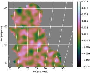
(b) $\kappa^{\rm KS}$ $B$-mode with no local rotations

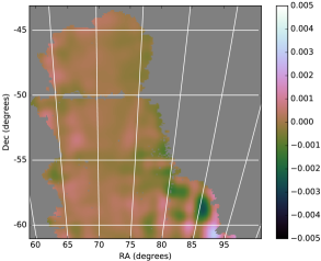
(c) Difference between $\kappa^{\rm KS}$ $E$-mode with and without local rotations

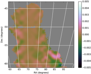
(d) Difference between $\kappa^{\rm KS}$ $B$-mode with and without local rotations

Figure 10: Plot to show the importance of applying the local rotations to real data when performing projections. We project the DES SV data using the sinusoidal projection considered by the DES collaboration. However, in this case we do not apply the necessary rotations to the galaxy shapes. Panel (a) and (b) show the results when no rotation is applied, while panels (c) and (d) show the error introduced by not applying the local rotations, i.e. the differences with the maps shown in Fig. 6(a) and Fig. 6(b).

References

- Aghanim et al. (2003) Aghanim N., Kunz M., Castro P.G., Forni O., 2003, A&A, 406, 797, astro-ph/0301220
- Alsing et al. (2016) Alsing J., Heavens A., Jaffe A.H., Kiessling A., Wandelt B., Hoffmann T., 2016, MNRAS, 455, 4452, arXiv:1505.07840
- Bacon & Taylor (2003) Bacon D.J., Taylor A.N., 2003, MNRAS, 344, 1307, astro-ph/0212266
- Bartelmann & Schneider (2001) Bartelmann M., Schneider P., 2001, Phys. Rep, 340, 291, astro-ph/9912508
- Becker et al. (2016) Becker M.R., et al., 2016, PRD, 94, 2, 022002, arXiv:1507.05598
- Brouwer et al. (2016) Brouwer M.M., et al., 2016, MNRAS, 462, 4451, arXiv:1604.07233
- Bunn et al. (2003) Bunn E.F., Zaldarriaga M., Tegmark M., de Oliveira-Costa A., 2003, PRD, 67, 2, 023501, astro-ph/0207338
- Castro et al. (2005) Castro P.G., Heavens A.F., Kitching T.D., 2005, PRD, 72, 2, 023516, astro-ph/0503479
- Chang et al. (2015) Chang C., et al., 2015, Physical Review Letters, 115, 5, 051301, arXiv:1505.01871
- Clowe et al. (2006) Clowe D., Bradač M., Gonzalez A.H., Markevitch M., Randall S.W., Jones C., Zaritsky D., 2006, ApJ L., 648, L109, astro-ph/0608407
- Coles & Chiang (2000) Coles P., Chiang L.Y., 2000, Nature, 406, 376, astro-ph/0006017
- Crittenden et al. (2001) Crittenden R.G., Natarajan P., Pen U.L., Theuns T., 2001, ApJ, 559, 552, astro-ph/0009052
- Crittenden et al. (2002) Crittenden R.G., Natarajan P., Pen U.L., Theuns T., 2002, ApJ, 568, 20, astro-ph/0012336
- de Jong et al. (2013) de Jong J.T.A., Verdoes Kleijn G.A., Kuijken K.H., Valentijn E.A., 2013, Experimental Astronomy, 35, 25, arXiv:1206.1254
- Flaugher et al. (2015) Flaugher B., et al., 2015, AJ, 150, 150, arXiv:1504.02900
- Goldberg et al. (1967) Goldberg J.N., Macfarlane A.J., Newman E.T., Rohrlich F., Sudarshan E.C.G., 1967, J. Math. Phys., 8, 11, 2155
- Górski et al. (2005) Górski K.M., Hivon E., Banday A.J., Wandelt B.D., Hansen F.K., Reinecke M., Bartelmann M., 2005, ApJ, 622, 759, astro-ph/0409513
- Green (2011) Green D.A., 2011, Bulletin of the Astronomical Society of India, 39, 289, 1108.5083
- Heavens (2009) Heavens A., 2009, Nuclear Physics B Proceedings Supplements, 194, 76, arXiv:0911.0350
- Heymans et al. (2012) Heymans C., et al., 2012, MNRAS, 427, 146, arXiv:1210.0032
- Hirata & Seljak (2004) Hirata C.M., Seljak U., 2004, PRD, 70, 6, 063526, astro-ph/0406275
- Hobson et al. (1998) Hobson M., Jones A., Lasenby A., 1998, MNRAS, 309, 125, astro-ph/9810200
- Jullo et al. (2007) Jullo E., Kneib J.P., Limousin M., Elíasdóttir Á., Marshall P.J., Verdugo T., 2007, New Journal of Physics, 9, 447, arXiv:0706.0048
- Jullo et al. (2014) Jullo E., Pires S., Jauzac M., Kneib J.P., 2014, MNRAS, 437, 3969, 1309.5718
- Kaiser & Squires (1993) Kaiser N., Squires G., 1993, ApJ, 404, 441
- Kamionkowski et al. (1997) Kamionkowski M., Kosowsky A., Stebbins A., 1997, PRD, D55, 7368, astro-ph/9611125
- Kaufman et al. (2016) Kaufman J.P., Keating B.G., Johnson B.R., 2016, MNRAS, 455, 1981, arXiv:1409.8242
- Kilbinger (2015) Kilbinger M., 2015, Reports on Progress in Physics, 78, 8, 086901, arXiv:1411.0115
- Kirk et al. (2015) Kirk D., et al., 2015, Space Science Reviews, 193, 139, 1504.05465
- Kitching et al. (2016) Kitching T.D., Alsing J., Heavens A.F., Jimenez R., McEwen J.D., Verde L., 2016, ArXiv e-prints, arXiv:1611.04954
- Kratochvil et al. (2012) Kratochvil J.M., Lim E.A., Wang S., Haiman Z., May M., Huffenberger K., 2012, PRD, 85, 10, 103513, arXiv:1109.6334
- Lanusse et al. (2016) Lanusse F., Starck J.L., Leonard A., Pires S., 2016, A&A, 591, A2, arXiv:1603.01599
- Laureijs et al. (2011) Laureijs R., et al., 2011, ArXiv e-prints, arXiv:1110.3193
- Leistedt et al. (2017) Leistedt B., McEwen J.D., Büttner M., Peiris H.V., 2017, MNRAS, 466, 3, 3728, arXiv:1605.01414
- Leistedt et al. (2013) Leistedt B., McEwen J.D., Vandergheynst P., Wiaux Y., 2013, A&A, 558, A128, 1, arXiv:1211.1680
- Leonard et al. (2012) Leonard A., Dupé F.X., Starck J.L., 2012, A&A, 539, A85, arXiv:1111.6478
- Leonard et al. (2014) Leonard A., Lanusse F., Starck J.L., 2014, MNRAS, 440, 1281, arXiv:1308.1353
- Lin & Kilbinger (2015a) Lin C.A., Kilbinger M., 2015a, A&A, 576, A24, arXiv:1410.6955
- Lin & Kilbinger (2015b) Lin C.A., Kilbinger M., 2015b, A&A, 583, A70, arXiv:1506.01076
- Lin et al. (2016) Lin C.A., Kilbinger M., Pires S., 2016, A&A, 593, A88, arXiv:1603.06773
- Liu & Hill (2015) Liu J., Hill J.C., 2015, PRD, 92, 6, 063517, arXiv:1504.05598
- LSST Science Collaboration et al. (2009) LSST Science Collaboration, et al., 2009, ArXiv e-prints, arXiv:0912.0201
- Marinucci & Peccati (2011) Marinucci D., Peccati G., 2011, Random Fields on the Sphere: Representation, Limit Theorem and Cosmological Applications, Cambridge University Press
- Massey et al. (2004) Massey R., et al., 2004, AJ, 127, 3089, astro-ph/0304418
- Massey et al. (2007) Massey R., et al., 2007, Nature, 445, 286, astro-ph/0701594
- Massey et al. (2015) Massey R., et al., 2015, MNRAS, 449, 3393, arXiv:1504.03388
- McEwen et al. (2005) McEwen J.D., Hobson M.P., Lasenby A.N., Mortlock D.J., 2005, MNRAS, 359, 1583, astro-ph/0406604
- McEwen et al. (2015) McEwen J.D., Leistedt B., Büttner M., Peiris H.V., Wiaux Y., 2015, IEEE TSP, submitted, arXiv:1509.06749
- McEwen & Wiaux (2011) McEwen J.D., Wiaux Y., 2011, IEEE TSP, 59, 12, 5876, arXiv:1110.6298
- Mediavilla et al. (2016) Mediavilla E., Muñoz J.A., Garzón F., Mahoney T.J., 2016, Astrophysical Applications of Gravitational Lensing, Cambridge University Press
- Munshi et al. (2011) Munshi D., Kitching T., Heavens A., Coles P., 2011, MNRAS, 416, 1629, arXiv:1012.3658
- Munshi et al. (2008) Munshi D., Valageas P., van Waerbeke L., Heavens A., 2008, Phys. Rep, 462, 67, astro-ph/0612667
- Munshi et al. (2012) Munshi D., van Waerbeke L., Smidt J., Coles P., 2012, MNRAS, 419, 536, arXiv:1103.1876
- Newman & Penrose (1966) Newman E.T., Penrose R., 1966, J. Math. Phys., 7, 5, 863
- Peel et al. (2016) Peel A., Lin C.A., Lanusse F., Leonard A., Starck J.L., Kilbinger M., 2016, ArXiv e-prints, arXiv:1612.02264
- Petri et al. (2013) Petri A., Haiman Z., Hui L., May M., Kratochvil J.M., 2013, PRD, 88, 12, 123002, arXiv:1309.4460
- Pichon et al. (2010) Pichon C., Thiébaut E., Prunet S., Benabed K., Colombi S., Sousbie T., Teyssier R., 2010, MNRAS, 401, 705, arXiv:0901.2001
- Plaszczynski et al. (2012) Plaszczynski S., Lavabre A., Perotto L., Starck J.L., 2012, A&A, 544, A27, 1201.5779
- Price et al. (2020) Price M.A., Cai X., McEwen J.D., Pereyra M., Kitching T.D., LSST Dark Energy Science Collaboration, 2020, MNRAS, 492, 1, 394, 1812.04017
- Price et al. (2021) Price M.A., McEwen J.D., Cai X., Kitching T.D., Wallis C.G.R., 2021, MNRAS, ISSN 0035-8711, stab1983
- Price et al. (2021) Price M.A., McEwen J.D., Pratley L., Kitching T.D., 2021, MNRAS, 500, 4, 5436, 2004.07855
- Schneider (2005) Schneider P., 2005, ArXiv Astrophysics e-prints, astro-ph/0509252
- Scoville et al. (2007) Scoville N., et al., 2007, ApJ S., 172, 1, astro-ph/0612305
- Seitz & Schneider (1995) Seitz C., Schneider P., 1995, A&A, 297, 287, astro-ph/9408050
- Simon (2013) Simon P., 2013, A&A, 560, A33, arXiv:1203.6205
- Simon et al. (2009) Simon P., Taylor A.N., Hartlap J., 2009, MNRAS, 399, 48, arXiv:0907.0016
- Spergel et al. (2015) Spergel D., et al., 2015, ArXiv e-prints, arXiv:1503.03757
- Szepietowski et al. (2014) Szepietowski R.M., Bacon D.J., Dietrich J.P., Busha M., Wechsler R., Melchior P., 2014, MNRAS, 440, 2191, arXiv:1306.5324
- Taylor (2001) Taylor A.N., 2001, ArXiv, astro-ph/0111605
- Taylor et al. (2004) Taylor A.N., et al., 2004, MNRAS, 353, 1176, astro-ph/0402095
- Van Waerbeke et al. (2013) Van Waerbeke L., et al., 2013, MNRAS, 433, 3373, arXiv:1303.1806
- VanderPlas et al. (2011) VanderPlas J.T., Connolly A.J., Jain B., Jarvis M., 2011, ApJ, 727, 118, arXiv:1008.2396
- Varshalovich et al. (1989) Varshalovich D.A., Moskalev A.N., Khersonskii V.K., 1989, Quantum theory of angular momentum, World Scientific, Singapore
- Vielva et al. (2004) Vielva P., Martínez-González E., Barreiro R.B., Sanz J.L., Cayón L., 2004, ApJ, 609, 22, astro-ph/0310273
- Vikram et al. (2015) Vikram V., et al., 2015, PRD, 92, 2, 022006, arXiv:1504.03002
- Wallis et al. (2016) Wallis C.G.R., Wiaux Y., McEwen J.D., 2016, IEEE TIP, submitted, arXiv:1608.00553
- Zaldarriaga & Seljak (1997) Zaldarriaga M., Seljak U., 1997, PRD, 55, 4, 1830, astro-ph/9609170
- Zuntz et al. (2015) Zuntz J., et al., 2015, Astronomy and Computing, 12, 45, arXiv:1409.3409