Deep Architectures for Modulation Recognition

Abstract

We survey the latest advances in machine learning with deep neural networks by applying them to the task of radio modulation recognition. Results show that radio modulation recognition is not limited by network depth and further work should focus on improving learned synchronization and equalization. Advances in these areas will likely come from novel architectures designed for these tasks or through novel training methods.

I Introduction

Deep neural networks have been pushing recent performance boundaries for a variety of machine learning tasks in fields such as computer vision, natural language processing, and speaker recognition. Recently researchers in the wireless communications field have started to apply deep neural networks to cognitive radio tasks with some success [13, 12, 10]. In particular it has been shown that relatively simple convolutional neural networks outperform algorithms with decades of expert feature searches for radio modulation [13]. This paper provides an introduction to deep neural networks for the cognitive radio task of modulation recognition, compares several state of the art methods in other domains, and experiments with learning techniques.

Deep neural networks are large function approximations comprised of a series of layers, where each layer represents some transform from input to output activations based on a parametric transfer function with some set of learned weights. Each layer is typically a known linear function with adjustable parameters and a non-linear activation function such that the resulting function composition can be highly non-linear [3]. Function parameters in deep neural networks are typically trained with a gradient descent optimizer from some loss function computed on the output of the network. For a multi-class classification task such as modulation recognition the objective function is often categorical cross-entropy (eq. 1). Categorical cross-entropy is a measure of difference between two probability distributions. For deep learning classification tasks the probability distribution is usually a softmax (eq. 2) of the output of the classifier network which is then converted to a one-hot encoding for classification purposes [3]. The error is calculated in what is known as the forward-pass and weights are adjusted using the chain rule to find error contribution for each parameter in what is known as the backward-pass. This kind of network output layer, optimization and loss function have been used very successfully for multi-class vision tasks such as object recognition on the Imagenet dataset [7].

$$H(p,q)=\Sigma_{x}p(x)\log q(x)$$ (1)

$$\sigma(z)_{j}=\frac{e^{z_{j}}}{\Sigma^{K}_{k=1}e^{z_{k}}}\quad\mathrm{for}\ j=1,...,K$$ (2)

Applying deep neural networks to solve well-known problem types, such as classification, is a matter of

• selecting a network architecture and hyper-parameters

• training the network to select weights which minimize loss

• applying it to the problem at hand

There are several well established network architectures including multi-layer perceptrons, many variations of convolutional networks, and recurrent networks. Although the goal of machine learning is to develop generalized techniques the current state of the art network types still seem to be application specific. For example, Google views Convolutional Long short-term Deep Neural Networks (CLDNN) to be worthy of patenting even though it is only used in their voice processing research. The state of the art in image recognition uses variants of the inception architecture, residual networks, and other architectures that enable many combinations of convolutional layers, while managing the combinatorial complexity of weights and activations. We discuss these methods in greater detail in the next section.

Before applying deep neural networks to wireless communications signals it is worth reviewing the state of the art for other application areas. The next section will review deep neural network architecture and learning advances that are likely to be valid and useful for wireless communications applications. Following the review of interesting deep architectures and training methods, results are in section III and a discussion in section IV.

I-A Neural Network Architectures

The common element in all state of the art deep neural networks is the use of convolutional layers. A convolutional layer consists of $N_{f}$ convolutional filters. The use of convolutional layers started for image and hand-writing recognition to provide feature translation invariance [8]. The use of convolutional filters in neural networks may be slightly different than expected for someone already familiar with FIR filters and DSP at least partially due to the use of activation functions in neural networks. Convolutions in neural networks are typically very small (1x1 through 5x5 are common sizes in image processing). In typical DSP applications filters are very wide (many taps/high order) rather than deep (small taps, but cascaded). Modern methods of implementing these filters, such as polyphase filterbanks, typically provide ways to reduce the width of filters for computational or latency reasons. The transfer function for a standard convolutional layer [9] is given below in equation 3, where $y_{i}$ is the output feature map for the $i$th filter, $b$ and $k$ represent learned bias and filter weight parameters, $x_{i}$ represents the input activations, $\ast$ denotes the convolution operation, and $f(..)$ denotes a (typically non-linear) activation function such as a rectified linear unit (ReLU) or sigmoid.

$$y_{i}=f\left(b_{j}+\Sigma_{i}k_{ij}\ast x_{i}\right)$$ (3)

A visible trend in neural networks for image processing is building deeper networks to learn more complex functions and hierarchical feature relationships [2, 1]. Deep networks enable more complex functions to be learned more readily from raw data than shallower networks with the same number of parameters [1, 18]; however, depth in neural networks is widely believed to be limited by unstable gradients that either explode or vanish in earlier or later layers in the network. This problem has been improved in recent years by the use of gradient normalization in optimizers as well as non-linearities which do not exacerbate the vanishing gradient problem such as rectified linear units (ReLUs). As a result several important architectures have been used to win competitions such as ImageNet by increasing depth that we will look at for improving radio modulation recognition.

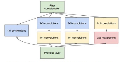
The inception architecture used in GoogLenet [17] is one successful approach to increasing network depth and ability to generalize to feature of differing scales while still managing complexity. This network consists of repeated inception modules. Each inception module (shown in figure 1), contains four parallel paths with the output being the concatenation of the four parallel outputs. The first path is a bank of 1x1 convolutions that forward along selected information. The 1x1 convolutions are a form of selective highway networks that simply pass information forward with no transformation. The second and third paths are 1x1 convolutions followed by a bank of 3x3 and 5x5 convolutions to provide multiple scales of feature detection. Finally, the last parallel path is a 3x3 pooling layer followed by 1x1 convolutions. Intermediate inception modules in the network are connected to softmax classifiers that contribute to the network’s global loss for training. These classifiers are believed to help in preventing vanishing gradients.

Figure 1: Inception Unit diagram from [17], generalizing to feature learning of multiple scales while also managing model complexity.

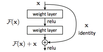
Another approach to increasing depth uses architectures that forward information untouched across layers. The best approach so far, which won ImageNet 2015, is residual networks [4]. A residual network adds one layer’s output to the output of the layer two layers deeper (as shown in figure 2). This is known as a residual network because the forwarded information forces the network to learn a residual function as part of feature extraction. The residual network authors suggest that vanishing gradients are resolved by normalization techniques that have been widely adopted and that network depth is instead limited by training complexity of deep networks which can be simplified with residual functions.

Figure 2: Residual network diagram from [4], allowing feature maps combinations from multiple source layers to select optimal architecture paths within a network.

CLDNNs are an approach for voice processing that operate on raw time-domain waveforms rather than expert voice features such as log-mel cepstrums [16, 15]. The architecture uses two convolutional layers followed by two recurrent layers made up of Long Short-Term Memory (LSTM) cells. LSTMs are a common recurrent network architecture consisting of several gates that control how long history is maintained [5]. CLDNNs can also have connections that bypass layers that are intended to provide a longer time context for the extracted features. For example, the original CLDNN forwards raw samples with the output of convolutional layers before the LSTM layers [15].

Inspired by the use of expert knowledge to guide network architectures such as convolutional networks and CLDNNs we experiment with a convolutional network that we will refer to as a convolutional matched filter. The rather simple idea is to take the general architecture of a typical communications receiver and build a neural network architecture that has similar parts. Communications receivers have a filter (typically matched to the transmitted pulse or wave shape), synchronizer, and sampler. Often the filter up front decimates to a small number of samples per symbol for the synchronizer which performs phase shifts to find the optimal sampling point. The sampler then slices to bits or emits audio for analog modulations. The neural network architecture analog to this is a convolutional layer with pooling followed by an LSTM.

I-B Neural Network Training

Hyper-parameters of a network such as learning rate, number of filters/feature maps per layer, filter size, and to some extent number of layers all affect network size and are hard to optimize. Recent research has attempted to optimize hyper-parameters as regular parameters that can be trained with backpropagation and gradient descent like network weights and biases. For this study we ignore training hyper-parameters and use the adam optimizer [6] which provides gradient normalization and momentum which reduces the importance of hyper-parameters like learning rate.

Guided by work that shows depth being more important than number of feature maps [2] we will establish a baseline convolutional network similar to that used in Radio Convolutional Modulation Networks [13]. Our first step is to tune the number of filters and number of taps per filter and view those as unimportant hyper-parameters for the remainder of experiments to test suitability of different architectures for RF data.

I-C Test Setup

II Technical Approach

We use the RadioML2016.10a dataset [12] as a basis for evaluating the modulation recognition task. The goal is to use a 128-sample complex (baseband I/Q) time-domain vector to identify the modulation scheme out of 11 possible classes. The 128 samples are fed in to the network in a 2x128 vector where the real and imaginary parts of the complex time samples are separated. The dataset uses a power delay profile, frequency selective fading, local oscillator offset, and additive white Gaussian noise with details of these effects in [12]. The dataset is labeled with both modulation type and SNR ground truth. We use the all-SNR top-1 classification accuracy as a single-number benchmark and show top-1 accuracy over SNR to compare techniques.

All models and training are done with the Keras deep learning library using the theano backend using an Nvidia GTX 1070 GPU.

We start with a network similar to the CNN2 network from [13]. This is the chosen baseline because results from [13] show significant improvement upon expert methods; any further improvements should be considered state of the art. The primary difference is we will use $nfilt$ filters of size 1x$taps$ on each layer. We will do a simple hyper-parameter optimization to

• find the best number of filters and filter size for RF modulation recognition

• test assumptions gained from other fields on network depth and filter size

III Results

III-A Baseline Convolution Network

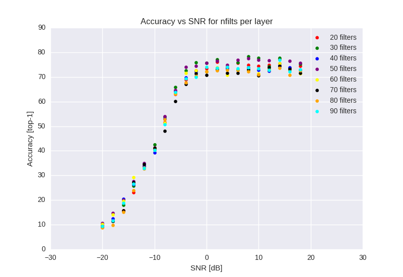
The baseline convolutional network has two convolution layers and a single dense layer before the softmax classifier. Each hidden layer has a rectified linear unit (ReLU) activation function and dropout of 50%. The first hyper parameter optimization is the size of our convolutional layers. Each layer will have 1x3 filters and we will vary the number of filters to find how many are needed. From [1, 18, 2] we expect that a large range in the number of filters will give similar performance before any overfitting will happen.

As expected there is a rather large window from about 30 to 70 filters per layer where performance is very similar. The top-1 classification accuracy for 20-90 filters in 10-filter increments is shown in figure 3. For the remaining experiments we will use 50 filters per layer.

Figure 3: Varying the number of filters per layer has small impact that is more noticeable at higher SNRs. Each network has 1x3 filters in a 2 convolutional layer network with 1 dense layer and a softmax classifier.

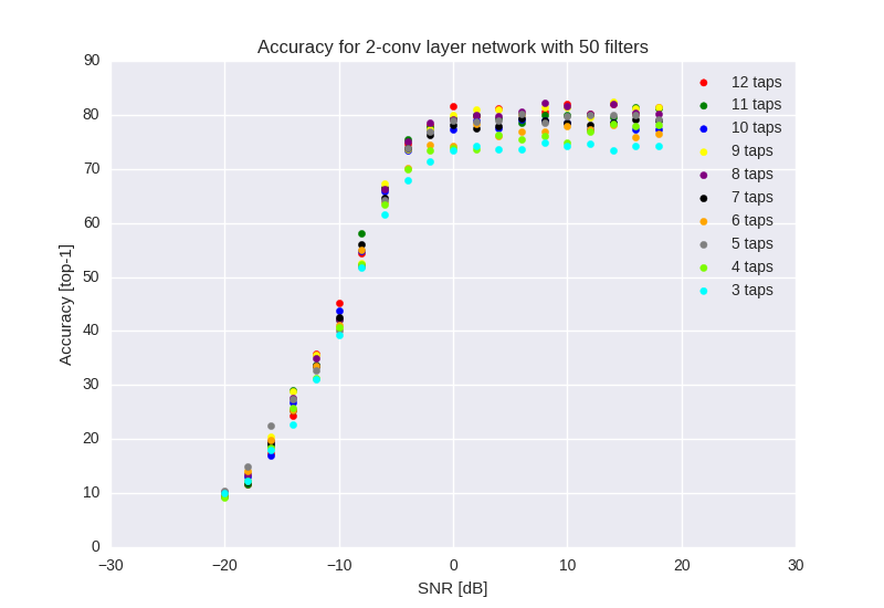
Next, we optimize the size of each filter. [2] suggests that the size of filters also has minimal impact, but based on expert knowledge of the radio domain and the dataset we expect 8-tap filters to be optimal. For this experiment we use a two-convolution layer network with a single hidden dense layer followed by the softmax classifier. The convolution layers each have 50 filters with a filter size of 1x$ntaps$ where $ntaps$ varies from 3 to 12.

Results from varying filter sizes for each convolution layer suggest that smaller filters are not as good as larger filters. We hypothesized based on expert knowledge of the dataset that 8-tap filters would be the best. It is difficult to distinguish a clear winner from the results per SNR graph in figure 4; however, the whole dataset classification accuracy shows that 7-12 taps all have similar performance around 61% with differences being statistically insignificant.

Figure 4: Varying the number of taps (filter size) in both convolutional layers. Lower numbers of taps are clearly inferior, but performance clusters as number of taps increases.

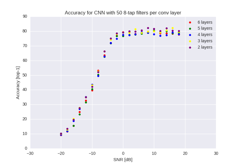
Finally, for purely convolutional networks we experiment with increasing network depth. For this experiment we use 50-tap convolutional layers with 1x8 filters. After the convolution layers we use a single hidden dense layer followed by a final dense softmax classifier. We start with a 2-convolutional-layer network and add convolution layers. Trends from deep learning suggest that adding more layers should improve classification performance until the gradient becomes unstable.

Varying the number of convolutional layers shows little to no improvement in classification accuracy. Accuracy over SNR for this task is shown in figure 5. This shows that there is no more feature depth for our network to learn. The data is not highly hierarchical to start with since the modulated data generally changes only the amplitude, frequency, or phase of a complex sinusoid; however, it is somewhat surprising that adding more convolutional layers does not appear to help reduce affects of noise at lower SNRs.

Figure 5: Varying the number of convolution layers in a DNN does not improve radio modulation recognition.

III-B Residual Networks

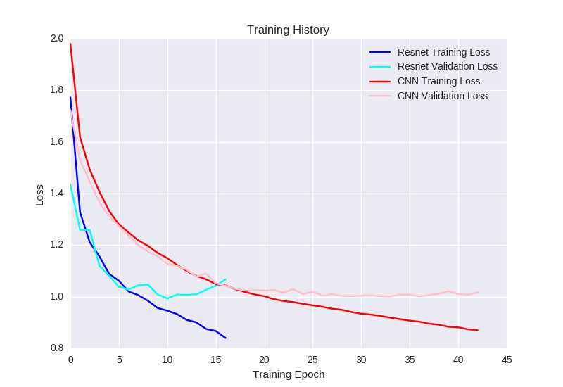
Although it is not surprising that adding more convolutional layers does not improve classification accuracy it is surprising that the classification and loss improvements plateau as soon as 2 or 3 convolutional layers. The original resnet insight is that deeper networks result in higher training loss which suggests higher training difficult rather than overfitting. Figure 6 shows that our hyper-parameter optimized CNN and a 9-layer residual network reaches similar loss, validation loss, and accuracy which is not shown; however, the residual network learns in fewer epochs. We also experimented with residual networks with 5-9 layers that all had similar performance and training times. This combined with our hyper-parameter search for ordinary CNN depth suggests we are not limited by network depth for radio learning tasks as much as we are limited by features purely CNN architectures can learn.

Figure 6: Training history showing the training loss and validation loss for a hyper-parameter optimized CNN and a 9-layer residual network. Both networks result in similar validation losses and training losses, but the residual network trains in fewer epochs.

III-C Inception Modules

Inception modules also do not improve radio modulation classification in our experiments here, using inception modules tuned for our dataset. The three branches used in each module are 50 1x1 filters, 50 1x3 filters, and 50 1x8 filters. The 1x3 and 1x5 filter branches also have 50 1x1 filters in front of them as shown in figure 7. The results for 1-4 inception modules in a network do not show any improvement over our hyper-parameter optimized CNN. Again, this suggests that we are not limited by depth or apparently by scale of filters.

Figure 7: An inception module for RF data showing convolution filter sizes. Each convolution layer has 50 filters.

III-D LSTM Networks

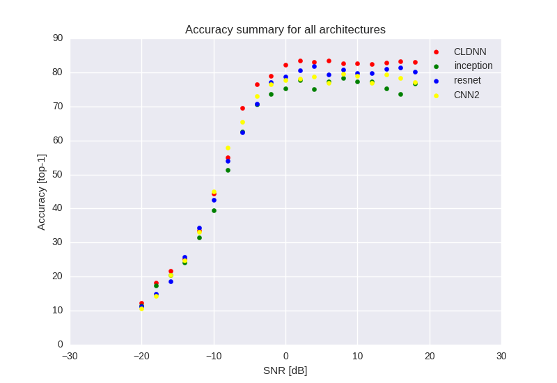
As the final architecture we test adding recurrent network layers, namely those comprised of LSTM units, for modeling temporal features. This approach is widely used in time-series applications and we expected that modulated baseband time-series may be similarly applicable. We tested two and three layer convolutions followed by recurrent layers in a CLDNN-type architecture with and without the forward/bypass connection before the recurrent layer. We found that the forward connection as a concatenation of the raw waveform and the convolutional output, shown in figure 8, results in better classification accuracy and more stable gradient descent than other architectures. Using a pooling layer that would create an architecture like the previously described convolutional matched filter detector does not help classification.

Figure 8: A CLDNN architecture for RF data. The output of the first 1x8 convolution layer is concatenated with the output of three 1x8 convolution layers before going to the LSTM.

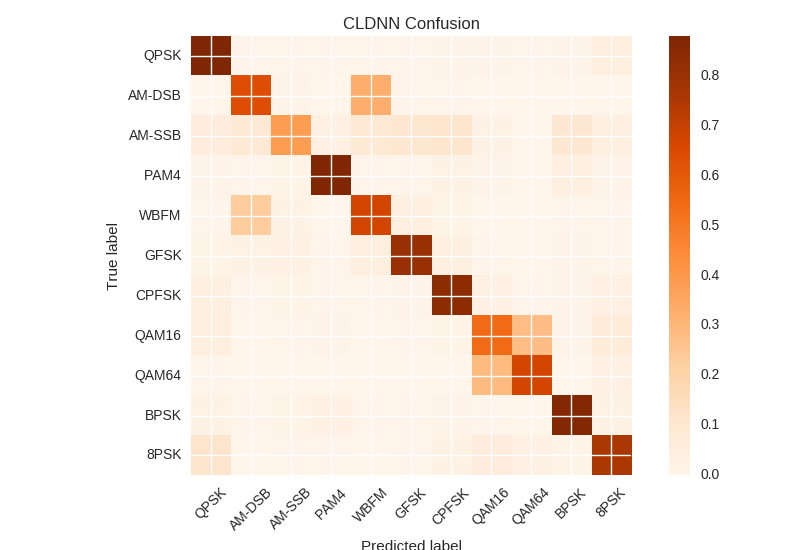
To further understand what limits classification accuracy we look at the confusion matrix for a CLDNN shown in figure 10. There are two primary areas of confusion. One is between the analog modulations and the other is between higher order QAMs. The analog modulations will be hard to address, but the QAMs can likely be improved on with better synchronization and reducing channel impairments.

Figure 9: A CLDNN consistently outperforms other network architectures for SNRs above -8dB.

Figure 10: The all-SNR confusion matrix for a CLDNN shows the most confusion between analog modulations and a separate confusion between higher order QAMs.

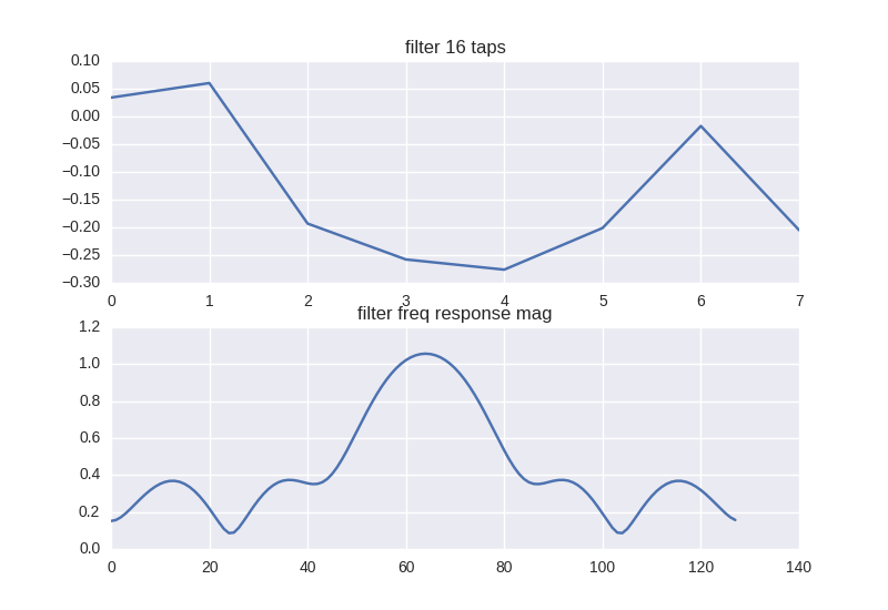
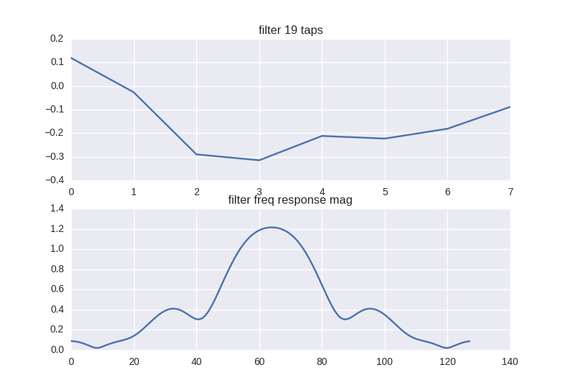
Gaining intuition on what the CLDNN is learning in each layer is important for guiding future work. To do this we plot the time and frequency representations of some filter taps. For the frequency response the filter taps are zero-padded with 100 zeros to get a 128-point FFT. Figs. 11(a) and 12(a) show two select filters from the first layer. The time-domain representations do not look particularly familiar to an expert eye; however the frequency responses do show shaped low-pass filters. Other filters that are not shown have frequency selective components, DC blockers, and sinc-like spectral shapes.

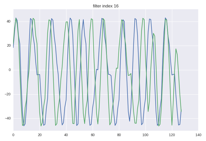
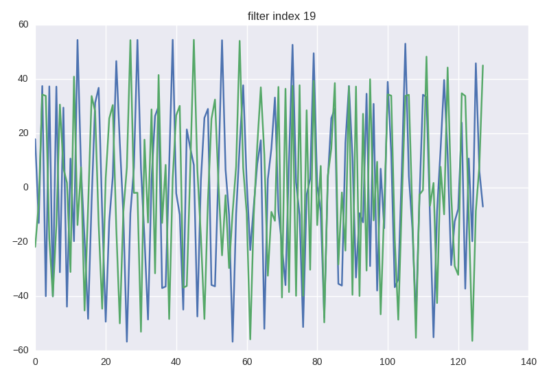
Another way to visualize these filters is to apply random data to them and perform a gradient ascent for the output of a particular filter which will converge on data that most activates a convolutional neuron [11]. Results for the selected two filters are shown in figs. 11(b) and 12(b). The resulting vectors look somewhat like crude PSK and FM/FSK modulations to an expert eye. The vectors also display some constant phase rotation that is present in our dataset due to the simulated channel model. It is important to note that these two filter visualizations were selected and not all filters appear meaningful to an expert.

(a) Time and frequency magnitude representations of a filter in the first convolutional layer of our trained CLDNN.

(b) Random data trained to maximally activate the filter, which winds up looking like BPSK.

(a) Time and frequency magnitude representations of a filter in the first convolutional layer of our trained CLDNN.

(b) Random data trained to maximally activate the filter, which winds up looking like FM or FSK modulation.

IV Discussion

Performance of deep neural networks in the radio domain does not seem to be limited by network depth the same way the image, natural language processing, and acoustic domains are. Although our experiments focused on modulation recognition as a benchmark task, we expect other radio machine learning tasks to be able to use similar network architectures. Further advances in deep learning for radio tasks will likely come from improved training methods and network architectures that can learn to transform RF data to remove effects of wireless channels, which neural network architectures are not designed for. One example that is currently being explored is the use of spatial transforms to equalize and synchronize incoming waveforms [14].

These experiments also focused on a dataset that is nominally bandwidth-normalized which is a poor assumption for signals captured from real radio transmissions. Future networks used in real-world applications will need to learn to either resample signals to be bandwidth normalized, or learn features for many bandwidths. Networks that can resample, synchronize, and remove non-linear channel distortions are all exciting future work for the field. We believe that as radio environments become increasingly complex, combining varying temporal behaviors of modulations, multi-modulation protocols and combining many radio emitters interoperating within a single band, many of these notions of hierarchy within deep networks will become increasingly important in allowing our networks to scale to cope with the complexity effectively as has been similarly shown in the vision domain within complex multi-object scenes.

References

- [1] Jimmy Ba and Rich Caruana. Do deep nets really need to be deep? In Z. Ghahramani, M. Welling, C. Cortes, N. D. Lawrence, and K. Q. Weinberger, editors, Advances in Neural Information Processing Systems 27, pages 2654–2662. Curran Associates, Inc., 2014.
- [2] David Eigen, Jason Tyler Rolfe, Rob Fergus, and Yann LeCun. Understanding deep architectures using a recursive convolutional network. CoRR, abs/1312.1847, 2013.
- [3] Ian Goodfellow, Yoshua Bengio, and Aaron Courville. Deep learning. Book in preparation for MIT Press, 2016.
- [4] Kaiming He, Xiangyu Zhang, Shaoqing Ren, and Jian Sun. Deep residual learning for image recognition. CoRR, abs/1512.03385, 2015.
- [5] Sepp Hochreiter and Jürgen Schmidhuber. Long short-term memory. Neural computation, 9(8):1735–1780, 1997.
- [6] Diederik P. Kingma and Jimmy Ba. Adam: A method for stochastic optimization. CoRR, abs/1412.6980, 2014.
- [7] Alex Krizhevsky, Ilya Sutskever, and Geoffrey E Hinton. Imagenet classification with deep convolutional neural networks. In Advances in neural information processing systems, pages 1097–1105, 2012.
- [8] Yann LeCun and Yoshua Bengio. The handbook of brain theory and neural networks. chapter Convolutional Networks for Images, Speech, and Time Series, pages 255–258. MIT Press, Cambridge, MA, USA, 1998.
- [9] Yann LeCun, Koray Kavukcuoglu, Clément Farabet, et al. Convolutional networks and applications in vision. In ISCAS, pages 253–256, 2010.
- [10] B. Migliori, R. Zeller-Townson, D. Grady, and D. Gebhardt. Biologically Inspired Radio Signal Feature Extraction with Sparse Denoising Autoencoders. ArXiv e-prints, May 2016.
- [11] Alexander Mordvintsev, Christopher Olah, and Mike Tyka. Inceptionism: Going deeper into neural networks. https://research.googleblog.com/2015/06/inceptionism-going-deeper-into-neural.html, July 2015.
- [12] Timothy O’Shea and Nathan West. Radio machine learning dataset generation with gnu radio. Proceedings of the GNU Radio Conference, 1(1), 2016.
- [13] Timothy J. O’Shea and Johnathan Corgan. Convolutional radio modulation recognition networks. CoRR, abs/1602.04105, 2016.
- [14] Timothy J. O’Shea, Latha Pemula, Dhruv Batra, and T. Charles Clancy. Radio transformer networks: Attention models for learning to synchronize in wireless systems. CoRR, abs/1605.00716, 2016.
- [15] T. N. Sainath, O. Vinyals, A. Senior, and H. Sak. Convolutional, long short-term memory, fully connected deep neural networks. In 2015 IEEE International Conference on Acoustics, Speech and Signal Processing (ICASSP), pages 4580–4584, April 2015.
- [16] Tara N Sainath, Ron J Weiss, Andrew Senior, Kevin W Wilson, and Oriol Vinyals. Learning the speech front-end with raw waveform cldnns.
- [17] Christian Szegedy, Wei Liu, Yangqing Jia, Pierre Sermanet, Scott E. Reed, Dragomir Anguelov, Dumitru Erhan, Vincent Vanhoucke, and Andrew Rabinovich. Going deeper with convolutions. CoRR, abs/1409.4842, 2014.
- [18] Gregor Urban, Krzysztof J Geras, Samira Ebrahimi Kahou, Ozlem Aslan, Shengjie Wang, Rich Caruana, Abdelrahman Mohamed, Matthai Philipose, and Matt Richardson. Do deep convolutional nets really need to be deep (or even convolutional)? arXiv preprint arXiv:1603.05691, 2016.