The kinematics of the white dwarf population from the SDSS DR12

Abstract

We use the Sloan Digital Sky Survey Data Release 12, which is the largest available white dwarf catalog to date, to study the evolution of the kinematical properties of the population of white dwarfs in the Galactic disc. We derive masses, ages, photometric distances and radial velocities for all white dwarfs with hydrogen-rich atmospheres. For those stars for which proper motions from the USNO-B1 catalog are available the true three-dimensional components of the stellar space velocity are obtained. This subset of the original sample comprises 20,247 objects, making it the largest sample of white dwarfs with measured three-dimensional velocities. Furthermore, the volume probed by our sample is large, allowing us to obtain relevant kinematical information. In particular, our sample extends from a Galactocentric radial distance $R_{\rm G}=7.8$ kpc to 9.3 kpc, and vertical distances from the Galactic plane ranging from $Z=-0.5$ kpc to 0.5 kpc. We examine the mean components of the stellar three-dimensional velocities, as well as their dispersions with respect to the Galactocentric and vertical distances. We confirm the existence of a mean Galactocentric radial velocity gradient, $\partial\langle V_{\rm R}\rangle/\partial R_{\rm G}=-3\pm 5$ km s^-1 kpc^-1. We also confirm North-South differences in $\langle V_{\rm z}\rangle$. Specifically, we find that white dwarfs with $Z>0$ (in the North Galactic hemisphere) have $\langle V_{\rm z}\rangle<0$, while the reverse is true for white dwarfs with $Z<0$. The age-velocity dispersion relation derived from the present sample indicates that the Galactic population of white dwarfs may have experienced an additional source of heating, which adds to the secular evolution of the Galactic disc.

1 Introduction

White dwarfs are the most usual stellar evolutionary endpoint, and account for about 97 per cent of all evolved stars — see, for instance, the comprehensive review of Althaus et al. (2010). Once the progenitor main-sequence star has exhausted all its available nuclear energy sources, it evolves to the white dwarf cooling phase, which for the coolest and fainter stars last for ages comparable to the age of the Galactic disc. Hence, the white dwarf population constitutes a fossil record of our Galaxy, thus allowing to trace its evolution. Moreover, the population of Galactic white dwarfs also conveys crucial information about the evolution of most stars. Furthermore, since the cooling process itself, as well as the structural properties of white dwarfs, are reasonably well understood (Althaus et al., 2010; Renedo et al., 2010), white dwarfs can be used to retrieve information about our Galaxy that would complement that obtained using other stars, like main sequence stars.

The ensemble properties of the white dwarf population are recorded in the white dwarf luminosity function, which therefore carries crucial information about the star formation history, the initial mass function, or the nature and history of the different components of our Galaxy — see the recent review of García-Berro & Oswalt (2016) for an extensive list of possible applications, as well as for updated references on this topic. Among these applications perhaps the most well known of them is that white dwarfs are frequently used as reliable cosmochronometers. Specifically, since the bulk of the white dwarf population has not had time enough to cool down to undetectability, white dwarfs provide an independent estimate of the age of the Galaxy (Winget et al., 1987; Garcia-Berro et al., 1988). But this is not the only interesting application of white dwarfs. In particular, the observed properties of the population of white dwarfs can also be employed to study the mass lost during the previous stellar evolutionary phases. Additionally, on the asymptotic giant branch white dwarf progenitors eject mass which has been enriched in carbon, nitrogen, and oxygen during the evolutionary stages. Hence, the progenitors of white dwarfs are significant contributors to the chemical evolution of the Galaxy. Finally, binary systems made of a main sequence star and a white dwarf can also be used to probe the evolution of the metal content of the Galaxy (Zhao et al., 2011; Rebassa-Mansergas et al., 2016).

All these studies are done analyzing the mass distribution of field white dwarfs. Several studies have focused on obtaining the mass distribution of Galactic white dwarfs. In particular, the mass distribution of white dwarfs of the most common spectral type — namely those with hydrogen-rich atmospheres, also known as DA white dwarfs — has been extensively investigated in recent years — see, for example Kepler et al. (2007) and Rebassa-Mansergas et al. (2015b), and references therein.

The first study of the kinematic properties of the white dwarf population was that of Sion et al. (1988), where a sample of over 1,300 degenerate stars from the catalog of McCook & Sion (1987) was employed. Since then, several studies have been done, focusing in different important aspects that can be obtained from the kinematical distributions, such as the identification of halo white dwarfs candidates (Liebert et al., 1989; Torres et al., 1998), the dark matter content of a potential halo population (Oppenheimer et al., 2001; Reid et al., 2001; Torres et al., 2002), or the possible existence of a major merger episode in the Galactic disc (Torres et al., 2001). However, the small sample sizes used in these studies prevented obtaining conclusive results. But this is not the only problem that these studies faced. Specifically, in addition to poor statistics, the major drawback of these works was the lack of reliable determinations of true three-dimensional velocities. The reason for this is that the surface gravity of white dwarf stars is so high that gravitational broadening of the Balmer lines is important. Thus, disentangling the gravitational redshift from the true Doppler shift is, in most of the cases, a difficult task. Consequently, determining the true radial velocity of white dwarfs require a model that predicts stellar masses and radii and hence, the value of the gravitational redshift. Even more, a sizable fraction of cool white dwarfs has featureless spectra, and hence for these stars only proper motions can be determined. All this precluded accurate measurements of the radial component of the velocity, and the assumption of zero radial velocity, or the method proposed by Dehnen & Binney (1998) were adopted in most studies — see, for instance, Sion et al. (2009) and Wegg & Phinney (2012), and references therein. More recently, Silvestri et al. (2001) presented a way to overcome this drawback. The authors studied a sample of white dwarfs in common proper motion binary systems. Among these pairs they selected a sub-sample in which the secondary star was an M dwarf, for which the sharp lines in its spectrum allowed to derive easily reliable radial velocities. Nevertheless, it was not until the ESO SNIa Progenitor surveY (SPY) project — see Pauli et al. (2006) and references therein — that radial velocities were measured for the first time with reasonable precisions. This was made because within this survey high resolution UVES VLT spectra were obtained for a sample of stars. Nevertheless, the sample of Pauli et al. (2006) only contained $\sim 400$ DA white dwarfs with radial velocities measurements better than $2\,{\rm km\,s^{-1}}$, of which they estimated that 2 per cent of stars were members of the Galactic halo and 7 per cent belonged to the thick disc.

In summary, the need of a complete sample, or at least statistically significant, with accurate measurements of true space velocities, distances, masses and ages, is crucial for studying the evolution of our Galaxy. In this sense, it is worth emphasizing that little progress has been done to use the Galactic white dwarf population to unravel the evolution of the Galactic disc studying the age-velocity relationship (AVR). Age-velocity diagrams reflect the slow increase of the random velocities with age due to the heating of the disc by massive objects. The term “disc heating” is often applied to the sum of the effects that may cause larger velocity dispersions in the population of disc stars. In principle, heating injects kinetic energy into the random component of the stellar motion over time. In order to understand the origin of the present assemblage of disc stars, it is necessary to quantify the kinematic properties of the populations in the disc and characterize the properties of their stars as accurately as possible. In other words, the space motions of the stars as a function of age allows us to probe the dynamical evolution of the Galactic disc.

Several heating mechanisms have been proposed in the last years. Among them we explicitly mention transient spiral arms (De Simone et al., 2004; Minchev & Quillen, 2006), giant molecular clouds, (Lacey, 1984; Hänninen & Flynn, 2002), massive black holes in the halo (Lacey & Ostriker, 1985), repeated disc impact of the original Galactic globular cluster population (Vande Putte et al., 2009), satellite galaxy mergers (Quinn et al., 1993; Walker et al., 1996; Velazquez & White, 1999; Villalobos & Helmi, 2008; Moster et al., 2010; House et al., 2011). Recently, Martig et al. (2014) studied the impact of different merger activity in the shape of the AVR in simulated disc galaxies and found that the shape of the AVR strongly depends on the merger history at low redshift for stars younger than 9 Gyr. A mechanism called radial mixing (Sellwood & Binney, 2002) was suggested as a possible source of disc heating (Schönrich & Binney, 2009; Loebman et al., 2011). However, Minchev et al. (2012) and Vera-Ciro et al. (2014) found that the contribution of radial mixing to disc heating is negligible in their simulations. Recently, Grand et al. (2016) used state-of-the-art cosmological magnetohydrodynamical simulations and found that the dominant heating mechanism is the bar, whereas spiral arms and radial migration are all subdominant in Milky Way-sized galaxies. They also found that the strongest source, though less prevalent than bars, originates from external perturbations from satellites/subhaloes of masses $\log_{\rm 10}(M/M_{\sun})\geq 10$.

Table 1: The stellar parameters, distances, proper motions, radial velocities, gravitational redshifts, plate-mjd-fib identifiers, spectral signal-to-noise ratios and ages for the complete sample of 20,247 SDSS hydrogen-rich white dwarfs used in this work. Ages 1, 2 and 3 are obtained using the initial-to-final mass relations of Catalán et al. (2008), Gesicki et al. (2014) and Ferrario et al. (2005), respectively. The table is published in its entirety in the online version of the paper.

Star	$T_{\mathrm{eff}}$	$M_{\mathrm{WD}}$	$\log\,g$	$d$	$\mu_{\mathrm{\alpha}}$	$\mu_{\mathrm{\delta}}$	$V_{\mathrm{r}}$	$V_{\mathrm{grav}}$	mjd	plt	fib	SN	Age 1	Age 2	Age 3
(SDSS)	(K)	$(M_{\odot})$	(dex)	(pc)	(mas)	(mas)	(km/s)	(km/s)					(Gyr)	(Gyr)	(Gyr)
J000006.75$-$004653.9	10793$\pm$ 244	0.680$\pm$0.130	8.137$\pm$0.205	234.28$\pm$ 35.94	$-$1.70$\pm$3.08	$-$1.31$\pm$3.08	40.81$\pm$20.27	37.15	52203	685	225	13.23	1.20${}^{+0.08}_{-3.56}$	1.16${}^{+0.07}_{-1.92}$	1.13${}^{+0.04}_{-2.87}$
J000012.32$-$005042.5	7570$\pm$ 361	0.603$\pm$0.426	8.016$\pm$0.678	233.72$\pm$120.07	$-$2.15$\pm$3.70	$-$5.49$\pm$3.70	$-$98.36$\pm$55.59	30.42	52902	1091	117	5.24	2.61${}^{+0.90}_{-2.74}$	2.27${}^{+1.23}_{-3.08}$	2.19${}^{+1.29}_{-3.16}$
J000022.87$-$000635.6	22550$\pm$ 658	0.417$\pm$0.033	7.430$\pm$0.103	641.58$\pm$ 57.94	15.53$\pm$3.01	4.67$\pm$3.01	$-$1.15$\pm$14.22	12.91	51791	387	166	19.32	—	—	—
J000034.06$-$052922.3	19640$\pm$ 167	0.505$\pm$0.017	7.730$\pm$0.037	221.78$\pm$ 7.17	85.34$\pm$2.48	$-$14.64$\pm$2.48	$-$10.97$\pm$ 6.04	20.06	54380	2624	261	55.48	—	—	—
J000051.84+272405.2	21045$\pm$ 402	0.606$\pm$0.042	7.960$\pm$0.075	476.17$\pm$ 27.28	11.55$\pm$3.10	$-$6.73$\pm$3.10	$-$25.33$\pm$11.74	28.59	54452	2824	272	23.33	1.32${}^{+0.50}_{-1.73}$	1.01${}^{+0.28}_{-0.83}$	0.93${}^{+0.25}_{-0.98}$
J000104.05+000355.8	13405$\pm$ 583	0.505$\pm$0.081	7.784$\pm$0.147	383.54$\pm$ 45.28	4.07$\pm$3.13	$-$9.67$\pm$3.13	$-$26.96$\pm$19.30	21.37	52203	685	490	14.46	—	—	—
J000110.09+273520.4	12681$\pm$ 470	0.488$\pm$0.106	7.750$\pm$0.200	607.84$\pm$ 97.89	$-$4.69$\pm$3.76	$-$8.66$\pm$3.76	$-$33.21$\pm$29.55	20.20	54452	2824	207	9.74	—	—	—
J000115.76+285647.2	13417$\pm$1244	0.509$\pm$0.113	7.792$\pm$0.201	588.26$\pm$ 95.54	9.29$\pm$3.62	$-$15.57$\pm$3.62	102.01$\pm$21.49	21.64	54452	2824	432	12.63	—	—	—
J000120.42$-$052140.8	7924$\pm$ 285	0.707$\pm$0.318	8.190$\pm$0.522	291.09$\pm$115.47	13.86$\pm$3.40	$-$60.69$\pm$3.40	$-$68.69$\pm$36.23	40.27	54327	2630	265	6.13	2.03${}^{+1.18}_{-3.41}$	1.99${}^{+1.21}_{-3.45}$	1.98${}^{+1.20}_{-3.46}$
J000126.85+272000.1	10023$\pm$ 46	0.566$\pm$0.044	7.933$\pm$0.067	119.80$\pm$ 6.21	113.18$\pm$2.72	$-$26.20$\pm$2.72	56.72$\pm$9.12	26.80	54368	2803	211	32.12	3.47${}^{+1.66}_{-1.41}$	2.31${}^{+0.78}_{-2.57}$	2.36${}^{+0.90}_{-2.52}$
J000135.06+244958.5	13668$\pm$2054	0.541$\pm$0.267	7.861$\pm$0.434	814.08$\pm$287.12	1.06$\pm$3.68	-5.11$\pm$3.68	61.06$\pm$ 44.00	24.13	54389	2822	273	7.70	—	—	—
J000208.73$-$050855.1	17505$\pm$ 521	0.501$\pm$0.056	7.740$\pm$0.114	659.22$\pm$ 63.46	—	—	75.28$\pm$ 27.01	20.21	54327	2630	273	14.07	—	—	—
J000216.02+120309.3	9913$\pm$ 933	0.907$\pm$0.426	8.512$\pm$0.839	678.84$\pm$487.93	—	—	102.98$\pm$110.92	65.72	55912	5649	467	2.05	1.69${}^{0.50}_{-1.03}$	1.66${}^{0.53}_{-1.00}$	1.64${}^{0.55}_{-0.98}$
J000228.15+235547.9	26801$\pm$ 428	0.559$\pm$0.026	7.820$\pm$0.070	731.77$\pm$ 39.05	13.01$\pm$3.05	0.07$\pm$3.05	12.98$\pm$ 12.39	23.42	54389	2822	251	29.81	3.43${}^{1.55}_{-0.86}$	2.04${}^{0.79}_{-2.25}$	2.27${}^{1.11}_{-2.02}$
J000236.49+254143.2	18330$\pm$ 886	0.585$\pm$0.116	7.930$\pm$0.200	874.14$\pm$134.61	-0.93$\pm$4.93	-0.89$\pm$4.93	70.85$\pm$ 43.43	27.14	54389	2822	371	7.55	1.94${}^{1.33}_{-2.42}$	1.31${}^{0.73}_{-3.05}$	1.23${}^{0.67}_{-3.13}$

From the observational point of view it is worth mentioning that some of the properties of the AVR are still controversial. For instance, Wielen (1977), Holmberg et al. (2007), and Aumer & Binney (2009) found that the stellar velocity dispersion increases steadily for all times, following a power law. In the case of the vertical velocity dispersion they found that $\sigma_{\rm z}\propto t^{\alpha}$, where $\alpha$ is close to 0.5. On the other hand, Dawson et al. (1984) found that the AVR rises fairly steeply for stars younger than 6 Gyr, thereafter becoming nearly constant with age. Another observational finding is that heating takes place for the first 2 to 3 Gyr, but then saturates when $\sigma_{\rm z}$ reaches $\sim 20$ km s^-1. This suggests that stars of higher velocity dispersion spend most of their orbital time away from the Galactic plane where the sources of heating lie (e.g. Stromgren, 1987; Quillen & Garnett, 2001; Soubiran et al., 2008). Seabroke & Gilmore (2007) found that vertical disc heating models that saturate after 4.5 Gyr are equally consistent with observations. The difficulty of obtaining precise ages for field stars (Soderblom, 2010), and selection effects in the different samples used by different authors might be responsible for the discrepancies mentioned above.

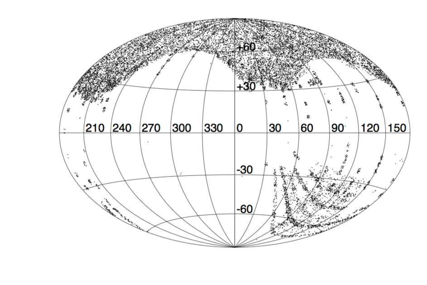
Figure 1: A Hammer-Aitoff projection in Galactic coordinates of the SDSS DR 12 spectroscopic plate distribution used in this work.

In this paper we use the sample of white dwarfs with hydrogen-rich atmospheres from the Sloan Digital Sky Survey (SDSS) data release (DR) 12, which is the largest catalog available to date, to determine velocity gradients in the $(R_{\rm G},\,Z)$ space. Moreover, since white dwarfs are excellent natural clocks we use them to compute accurate ages and in this way we determine the AVR in the solar vicinity. All this allows us to investigate the kinematic evolution of the Galactic disc. This paper is organized as follows. In Sect. 2 we describe the white dwarf catalog and we explain how we assess the quality of white dwarf spectra. Sect. 3 is devoted to explain how we derive effective temperatures and surface gravities, as well as their respective errors, and to discuss the corresponding distributions. We also present the set of derived masses, ages, distances, radial velocities and proper motions. This is later used in Sect. 4 where we present the velocity maps and age gradients. The AVR is discussed in Sect. 5, while in Sect. 6 we summarize our most important results and we draw our conclusions.

2 The white dwarf catalog

Modern large scale surveys have been very profficient at identifying white dwarfs. Among them we mention the Palomar Green survey (Liebert et al., 2005), the Kiso survey (Limoges & Bergeron, 2010), and the LAMOST spectroscopic survey of the Galactic Anti-Center (Rebassa-Mansergas et al., 2015a). However, it has been the SDSS (York et al., 2000; Alam et al., 2015) the survey that in recent years has significantly increased the number of known white dwarfs. Indeed, the SDSS has produced the largest spectroscopic sample of white dwarfs, and its latest release, the DR 12, contains more than 30,000 stars (Kepler et al., 2016). Because of its considerably larger size as compared to other available white dwarf catalogs, we adopt the SDSS catalog as the sample of study in this work. From this sample we select only white dwarfs with hydrogen dominated atmospheres, that is of the DA spectral type. For these white dwarfs radial velocities and the relevant stellar parameters can be derived using the technique described below. The Galactic coordinates of the 20,247 DA white dwarfs selected in this way are shown in Fig. 1, whereas Table 1 lists the stellar parameters, proper motions and radial velocities of these stars. This table is published in its integrity in machine-readable format. However, for obvious reasons, only a portion is shown here for guidance regarding its form and content.

2.1 Signal-to-noise ratio of the SDSS white dwarf spectra

Before providing details on how we measure the stellar parameters and radial velocities from the SDSS white dwarf spectra it is important to mention that these spectra are in several cases rather noisy. This is because white dwarfs are generally faint objects. Hence, the stellar parameters and radial velocities derived from their spectra often have large uncertainties. In order to select a clean DA white dwarf sample for the AVR of the Galactic disc we hence need to exclude all bad quality data. We will do this based on the signal-to-noise ratio (SNR) of the SDSS spectra, which is calculated for each spectrum in this section.

The featureless spectral region of the continuum in a white dwarf DA spectrum allows us to derive a statistical estimate of the SNR using a rather simple approach. This is done comparing the flux level (signal) within a particular wavelength range to the intrinsic noise of the spectrum in the same wavelength region. That is, we compute the ratio of the average signal to its standard deviation — see, for example, Rosales-Ortega et al. (2012).

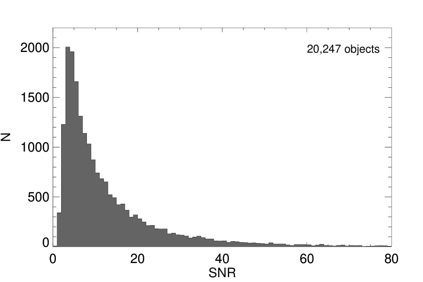
Figure 2: Distribution of the signal-to-noise ratios of the white dwarf spectra in the sample analyzed in this work. The distribution peaks at SNR$\,\sim\,$5, while the mean value is 13.2.

Table 2: The four selected central wavelength ($\lambda_{\rm C}$) regions, C1, C2, C3 and C4 respectively, and their wavelength widths ($\Delta\lambda$) for a statistical estimate of the signal-to-noise ratio in the SDSS spectra.

	$\lambda_{\rm C}$ (Å)	$\Delta\lambda$ (Å)
C1	4600	200
C2	5300	400
C3	6100	600
C4	6900	200

We defined four continuum bands centered at $\lambda_{\rm C}$ of width $\Delta\lambda$ (see Table 2) from the observed spectrum, $f(\lambda$). We applied a correction for the presence of a slope within the continuum band, where $\sigma_{\rm C}$ is the standard deviation in the difference between $f(\lambda$) and a linear fit to $f(\lambda$). We then calculated the statistical SNR for the four continuum bands employing the expression (SNR)${}_{\rm C_{i}}$ = $\mu_{\rm C_{i}}/\sigma_{\rm C_{i}}$, where $\mu_{\rm C_{i}}$ is the mean flux in the given continuum band and $\sigma_{\rm C_{i}}$ is the standard deviation of the flux within the given continuum band, dominated by noise instead of real features. We found that SNR${}_{\rm C1}>$SNR${}_{\rm C2}>$SNR${}_{\rm C3}>$SNR_C4, for all the spectra, as expected for these stars, where emergent flux appears in the blue wavelengths. We finally derived the continuum SNR of an observed spectrum as the average of the individual (SNR)${}_{\rm C_{i}}$ calculated for each of the pseudocontinuum bands, C1, C2, C3 and C4 respectively. Fig. 2 shows the histogram of the distribution of the statistical SNR for the total of 20,247 white dwarf spectra selected for this study. We found that half of the sample has a statistical SNR for the continuum larger than 12 while most of the spectra a SNR around 5.

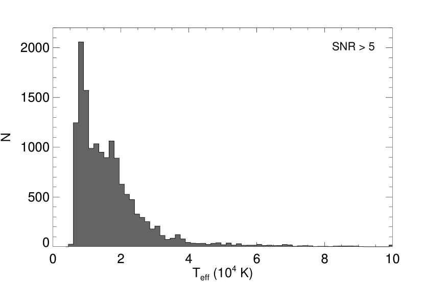
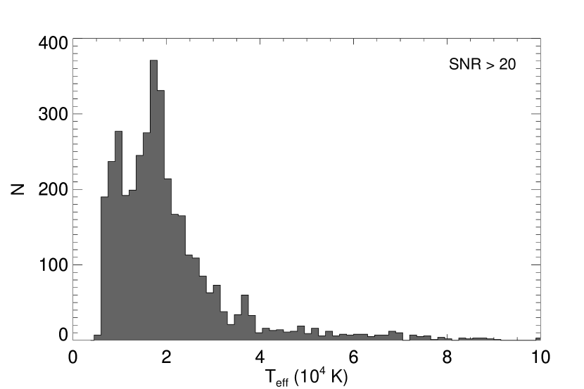
Figure 3: Distribution of effective temperatures for the SDSS DA white dwarf sample employed in this study. Most of the objects in the sample have effective temperatures between $7,000\,$K and $30,000\,$K. The left panel shows the distribution for white dwarfs with spectra with SNR$>$5, while the right panel displays the same distribution for stars with spectra with SNR$>$20.

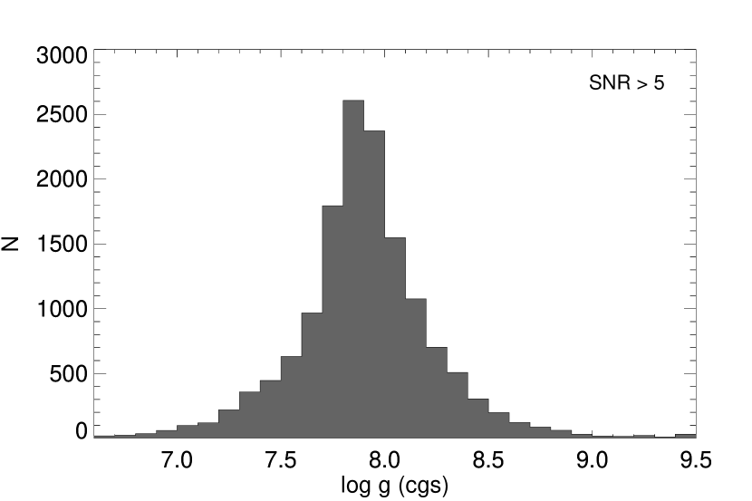
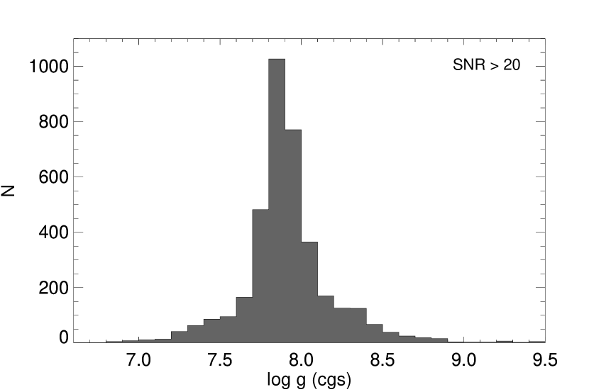
Figure 4: Distribution of surface gravities for the SDSS DA white dwarf sample employed in this study. The surface gravity distribution for the sample displays a narrow peak at around 7.8 dex. The left panel shows the distribution for white dwarfs with spectra SNR$>$5, while the right panel displays the same distribution for stars with spectra with SNR$>$20.

3 Distributions of stellar parameters

White dwarfs are classified into several different sub-types depending on their atmospheric composition. The most common of these sub-types are DA white dwarfs, which have hydrogen-rich atmospheres. They comprise $\sim$85 per cent of all white dwarfs — see, e.g., Kleinman et al. (2013). The most distinctive spectral feature of DA white dwarfs is the Balmer series. These lines are sensitive to both the effective temperature and the surface gravity. We fitted the Balmer lines sampled by the SDSS spectra with the one-dimensional model atmosphere spectra of Koester (2010), for which the parameterization of convection follows the mixing length formalism ML2/$\alpha=0.8$. In order to account for the higher-dimensional dependence of convection, which is important for cool white dwarfs, we applied the three-dimensional corrections of Tremblay et al. (2013).

3.1 Effective temperatures and surface gravities

Fig. 3 shows the distributions of effective temperatures for two sets of data. In the left panel the distribution of effective temperatures for a sub-sample of white dwarfs with spectra having SNR$>$5 is displayed, whereas the right panel shows the same distribution for those white dwarfs with spectra of an excellent quality, namely those with SNR$>$20. For those white dwarfs with spectra with SNR$>$5 the effective temperatures are within $6,000\,{\rm K}\,<$$T_{\mathrm{eff}}$$<\,100,000\,$K, but most white dwarfs have effective temperatures between 7,000 K and 30,000 K, while although for the sub-sample with SNR$>$20 the same is true, there is a secondary peak at $T_{\rm eff}\sim 10,000$ K. The origin of this peak remains unclear, but it is related to the longer cooling timescales of faint white dwarfs. However, a precise explanation of this peak must be addressed with detailed population synthesis studies, which are beyond the scope of this paper. Fig. 4 displays the distribution of surface gravities for both the sub-sample with SNR$>$5 (left panel) and that with SNR$>20$ (right panel). As can be seen, in both cases surface gravities ranges from 6.5 dex $<\log g<$ 9.5 dex with a narrow peak around 7.85 dex. These distributions are very similar to those presented by other authors using SDSS DA white dwarfs (e.g. Kleinman et al., 2013; Kepler et al., 2015). In summary, we conclude that the sub-sample of white dwarfs with SNR$>$20 is totally representative of the sample of white dwarfs. This sub-sample will be used below to derive in a reliable way the kinematical properties of the white dwarf population.

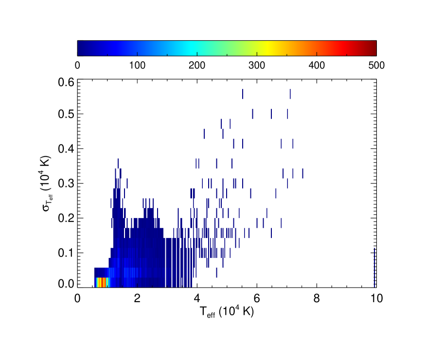
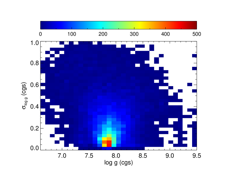
Figure 5: Distribution of uncertainties for both the effective temperatures (upper panel) and surface gravities (lower panel) for the SDSS DA white dwarf sample employed in this study. This distribution of errors corresponds to all white dwarfs with spectra having SNR$>$5.

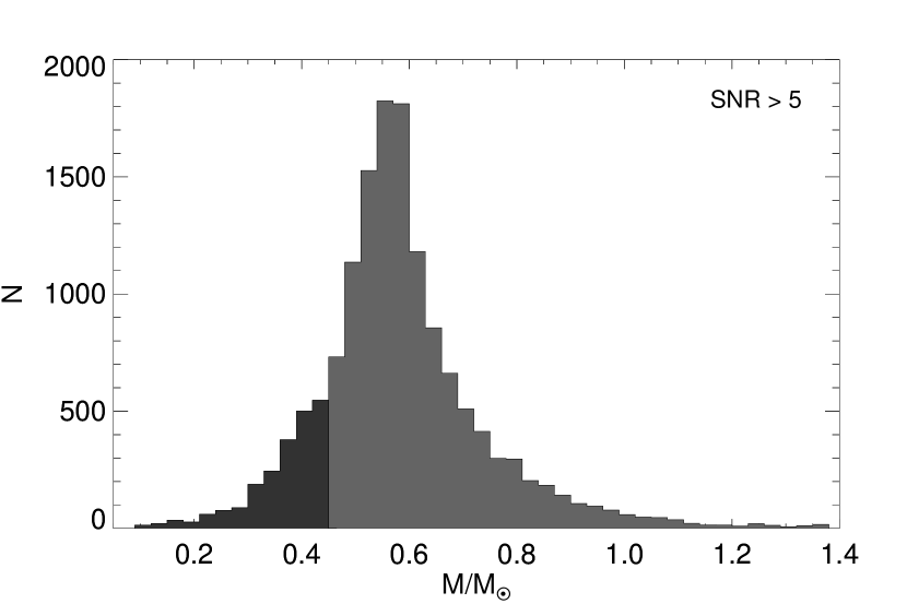
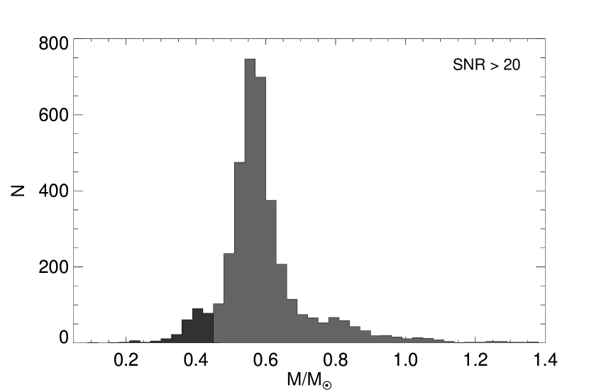
Figure 6: Mass distribution for the SDSS DA white dwarf sample employed in this study. The left panel shows the distribution for white dwarfs with spectra SNR$>$5, while the right panel displays the same distribution for stars with spectra with SNR$>$20. In both cases the distributions have a narrow peak at $\sim 0.55\,M_{\sun}$. The black shaded area shows white dwarfs with masses $M_{\rm WD}<0.45\,M_{\sun}$, which are thought to be formed through binary evolution (see text for more details).

Fig. 5 shows the distribution of errors of the effective temperatures as a function of the effective temperature for all 20,427 DA white dwarfs with spectra having SNR$>$5 (upper panel), and the corresponding distribution of uncertainties in surface gravities as a function of surface gravity (lower panel). It is worth noting that both distributions have very narrow peaks. Actually, the typical uncertainties peak around $\sigma_{T_{\rm eff}}\sim 200\,$K and $\sigma_{\log{\rm g}}\sim 0.15\,$dex. These values are comparable to those obtained in equivalent studies of this kind (Kleinman et al., 2013; Kepler et al., 2015).

We interpolated the measured effective temperatures and surface gravities on the cooling tracks of Althaus et al. (2010) and Renedo et al. (2010) to derive the white dwarf masses, radii, cooling ages and absolute $UBVRI$ magnitudes. The absolute magnitudes in the UBVRI system were converted into the $ugriz$ system using the equations of Jordi et al. (2006).

In passing we note that although white dwarfs cool down at almost constant radii, the radius (hence, the surface gravity) slightly evolves as time passes by. Consequently, mass determinations, along with the corresponding uncertainties, depend on both T_eff and $\log g$.

3.2 Mass distribution

In Fig. 6 we show the mass distribution for the white dwarf sub-sample with spectra with SNR$>$5 (left panel) and the sub-sample with SNR$>$20 (right panel). For the sample with spectra with SNR$>$5 the observed mass distribution exhibits a narrow peak with broad and flat tails which extend both to larger and smaller masses. The mean mass of the distribution is near $0.55\,M_{\sun}$. We found that most white dwarfs in this sample have mass uncertainties $\sigma_{M_{\rm WD}}<0.15\,M_{\sun}$. The sub-sample with SNR$>$20 shows a similar behavior, but although the mean mass of the distribution is essentially the same, the mass distribution is narrower, and the tails at low and high masses are much less evident. This is particularly true for white dwarfs with masses smaller than $0.45\,M_{\sun}$ — those that populate the black shaded area in this figure. This is a direct consequence of the better determination of white dwarf masses for the sub-sample with spectra with larger SNR.

Theoretical models predict that white dwarfs of masses below $0.45\,M_{\sun}$ have helium cores. The existence of such low-mass helium-core white dwarfs cannot be explained by single stellar evolution, as the main sequence lifetimes of the corresponding progenitors would be larger than the Hubble time. It is then expected that these low-mass white dwarfs are formed as a consequence of mass transfer episodes in binary systems, which lead to a common envelope phase, and hence to a dramatic decrease of the binary orbit (Liebert et al., 2005; Rebassa-Mansergas et al., 2011). We therefore expect the vast majority of all low-mass (those with masses $\leq 0.45\,M_{\sun}$) white dwarfs in our sample to be members of close binaries.

Additionally, there is another potential source of close binary contamination in the white dwarf mass distribution, for masses above $0.45\,M_{\sun}$. Post-common-envelope binaries, typically including a carbon-oxygen core white dwarf, represent a noticeable fraction of the Galactic white dwarf population — see, e.g., Rebassa-Mansergas et al. (2012) and Camacho et al. (2014). Some of these systems are likely present in our sample when the companion is an unseen low-mass star or a second (less luminous) white dwarf. In those cases, the brighter and lower mass white dwarf will likely have experienced a mass loss episode. Badenes & Maoz (2012) and Maoz & Hallakoun (2016) estimated that the number of close binary systems represent $\sim 10$ per cent of the population.

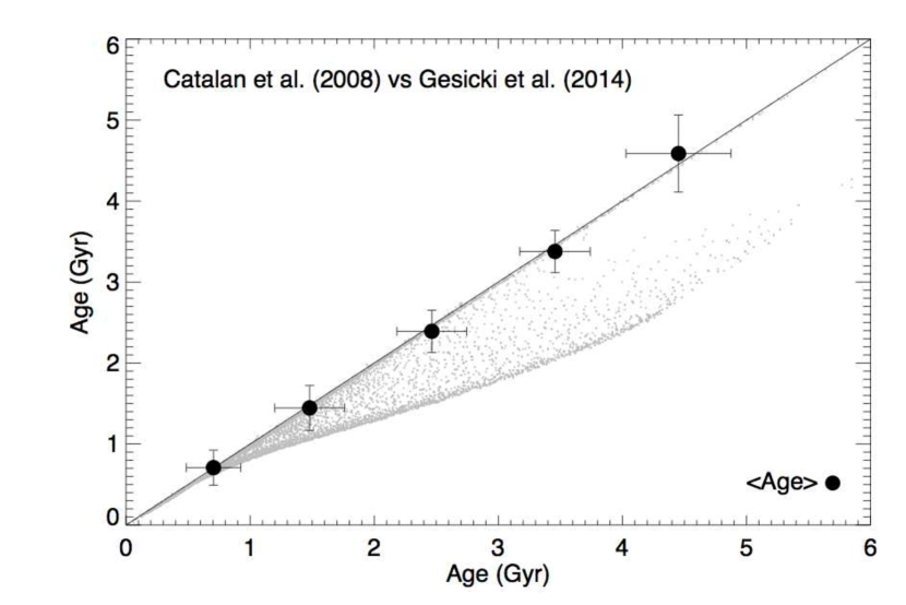
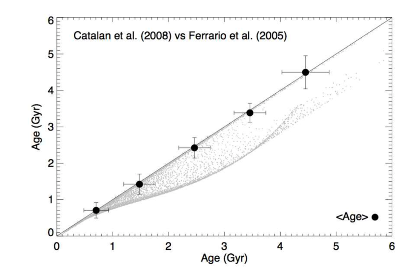
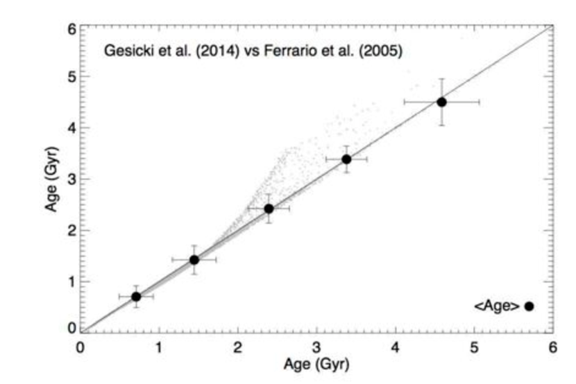
Figure 7: Comparison between the total ages of white dwarfs obtained using the IMFRs of Catalán et al. (2008), Ferrario et al. (2005) and Gesicki et al. (2014). Note the impact of the different IMFRs in the final estimated individual ages.

3.3 Ages

The age of a white dwarf is computed as the sum of its cooling age plus the main sequence lifetime of its progenitor. Using the white dwarf effective temperatures and surface gravities obtained in Sect. 3.1 we interpolated these values on the cooling tracks of Renedo et al. (2010) to obtain the corresponding cooling ages. To obtain their main sequence progenitor lifetimes an initial-to-final mass relation (IFMR) — i.e., the relationship between the white dwarf mass and the mass of its main sequence progenitor — must be adopted. Given that the currently available IFMRs suffer from relatively large observational uncertainties, especially for white dwarf with masses below $0.55\,M_{\sun}$, here we adopted three different relationships. More specifically, we used the semi-empirical IFMR of Catalán et al. (2008) as our reference case. However, to assess the uncertainties in the cooling ages we also employed the IFMRs of Ferrario et al. (2005) and Gesicki et al. (2014). All three IFMRs cover the range of white dwarf masses with carbon-oxygen cores. Even more, we only calculated ages for stars with masses larger than $0.55\,M_{\sun}$. Using these IFMRs we derived three independent values of the progenitor masses for each white dwarf. We then interpolated the progenitor masses in the solar-metallicity BASTI isochrones of Pietrinferni et al. (2004) and computed the time that the white dwarf progenitors spent on the main sequence, and thus the total age.

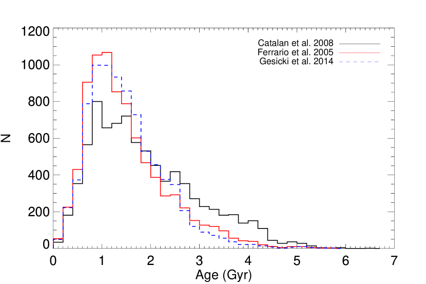
Figure 8: Age distributions using our three adopted IFMRs (Catalán et al., 2008; Ferrario et al., 2005; Gesicki et al., 2014). The three distributions show a clear peak at around 1 Gyr.

In Fig. 7 we compare the total ages obtained using different IFMRs for white dwarfs with spectra with SNR$>$5. As can be seen, although there is a sizable fraction of stars that have nearly equal ages, systematic effects arise when using the IFMRs derived by different authors. Thus, we turn our attention to quantify the impact of the different IFMRs on the ages of stars in our sample. In Fig. 7 we also show the average ages and standard deviations for our sample of white dwarfs when stars are grouped in bins of 1 Gyr duration. As can be seen the average ages are in excellent agreement with each other, and the standard deviations are substantially smaller than the size of the bin. This means that although the ages of individual white dwarfs may differ depending on the adopted IFMR, the average ages in each 1 Gyr bin are in good agreement. Thus, these ages can be safely employed to derive average structural properties of our Galaxy.

We also study the distribution of ages of white dwarfs in our sample. Fig. 8 shows the distribution of white dwarf ages for the three IFMRs already mentioned. The three distributions show a peak around 1 Gyr. However, for the distribution of ages obtained using the IFMRs of Ferrario et al. (2005) and Gesicki et al. (2014) the peak is narrower, whereas the distribution of ages obtained using the IFMR of Catalán et al. (2008) has a smaller peak and shows an extended tail with a significant number of white dwarfs with ages ranging from 2 to 5 Gyr. This is because the slope of the IFMR of Catalán et al. (2008) is steeper, and thus results in an extended age distribution. Finally, in all three cases there is a clear paucity of white dwarfs with ages larger than $\sim 6$ Gyr. This is because relatively massive white dwarfs older than $\sim 6$ Gyr are typically rather cool ($T_{\mathrm{eff}}$$<$ 7,000 K) and hence too faint and difficult to detect by the SDSS. Hence, we will not be able to probe the very first stages of the Galactic disc.

Finally, we emphasize that the age uncertainty for individual white dwarfs depends on both its mass (or, equivalently, the surface gravity) and its luminosity (namely, the effective temperature). We found that typical age uncertainties cluster around $\sigma_{\rm age}=0.5$ Gyr and that most of the SDSS DA white dwarfs in this study have $\sigma_{\rm age}<2.5$ Gyr. This final error budget may be slightly underestimated as we employed solar metallicity isochrones for all the objects, however this is a reasonable assumption for our local sample as most of the objects belong to the thin disc where a metallicity close to solar is the most common value for a sample between $R_{\rm G}=7$ kpc to 9 kpc, and vertical distances from the Galactic plane ranging from $Z=-0.5$ kpc to 0.5 kpc (Hayden et al., 2015).

3.4 Rest-frame radial velocities

We determined the radial velocities (RVs) from the observed SDSS spectra using a cross-correlation procedure originally described by Tonry & Davis (1979). We used 128 DA white dwarf model spectra (Koester, 2010) at the SDSS nominal spectral resolution. The models cover effective temperatures in the range $6,000\,$K to $80,000\,$K and surface gravities from 7.5 to 9 dex. We used the IRAF package rvsao (Kurtz & Mink, 1998).

The low spectral resolution and the low SNR (see Fig. 2) for most of SDSS DA white dwarf spectra together with the broad Balmer lines make deriving precise RVs a challenging task. Thus, to improve the RV determinations we implemented a Fourier filter. The aim of this filter is to suppress some of the low-frequency power, making the Balmer lines narrower. We also designed the filter for an optimal removal of photon noise at the high-frequency end of the spectrum. Also, to derive the RV uncertainties we used the cross-correlation coefficient ($r$), where $r$ is the ratio of the correlation peak height to the amplitude of the antisymmetric noise (Tonry & Davis, 1979). Fig. 9 shows the uncertainties from the cross-correlation in RV as a function of the SNR of the SDSS spectra for our 20,247 DA white dwarfs. For stars with SNR$<$5, $\sigma_{\rm RV}$ is always larger than $\sim 25$ km s^-1. For spectra with SNR larger than 20 we found $\sigma_{\rm RV}$$<$15 km s^-1.

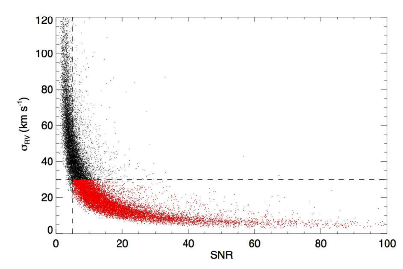
Figure 9: Uncertainties in RV as a function of SNR of the SDSS spectra for the our entire sample, a total of 20,247 objects. Objects with SNR$<$5 are associated to large uncertainties and are not considered in our analysis. All the white dwarf spectra with SNR$>$20 have $\sigma_{RV}<20\,$km s^-1.

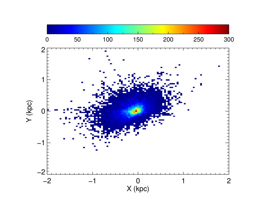
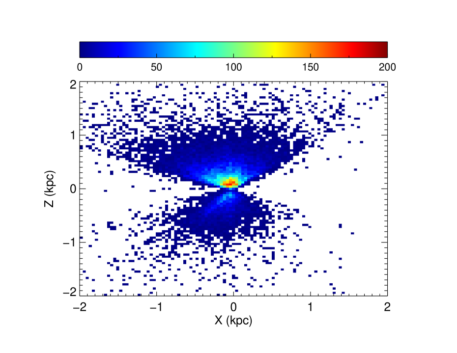
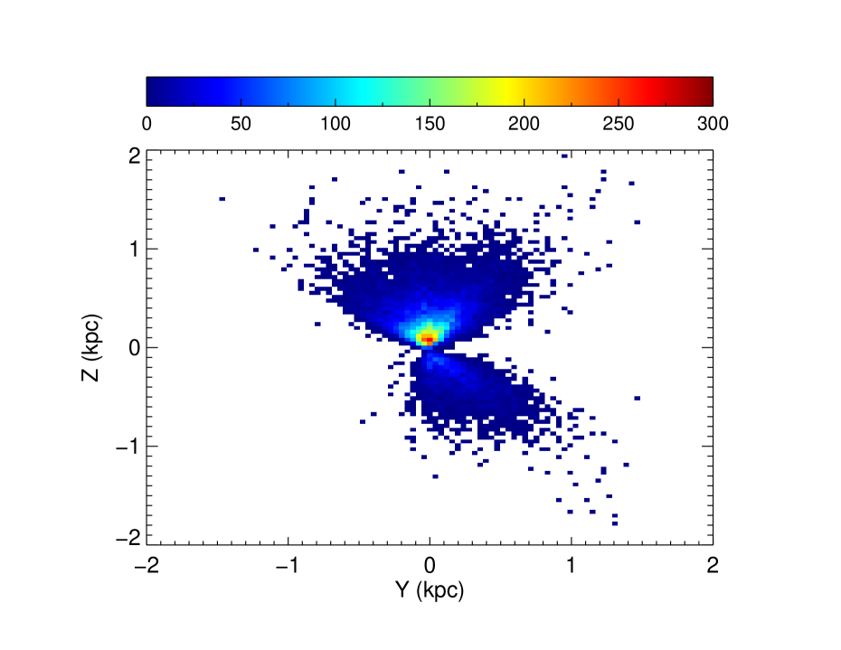
Figure 10: The $XYZ$ distribution of the white dwarf sample color coded according to the spatial density, see text for details.

The spectra of white dwarfs are affected by gravitational redshifts due to their high surface gravities. Thus, the velocities measured by the cross-correlation technique (hereafter RV_cross) are the sum of two individual components (Falcon et al., 2010), an intrinsic radial velocity component (RV) and the contribution of the gravitational redshift RV${}_{\rm grav}=GM/Rc$. In this expression $G$ is the gravitational constant, $c$ is the speed of light and $M$ and $R$ are the white dwarf mass and radius respectively. Note that these quantities are known for each star (see Sect. 3.1). Hence, the radial velocities of our SDSS DA white dwarfs are finally obtained as RV=RV${}_{\rm cross}-GM/Rc$. The error contribution from the gravitational redshift RV_grav has a typical value of 1.5 km s^-1, and all the sample has $\sigma$ $<$ 4 km s^-1 when SNR$>$20.

3.5 Distances and spatial distribution

We derived the distances to all SDSS DA white dwarfs from their distance moduli $M_{\mathrm{g}}-g-A_{\mathrm{g}}$, where $M_{\mathrm{g}}$ is the SDSS $g$-band absolute magnitude (see Sect. 3.1), $g$ is the SDSS $g$-band apparent magnitude and $A_{\mathrm{g}}$ is the $g$-band extinction. $A_{\mathrm{g}}=E(B-V)R_{\mathrm{g}}$, with $E(B-V)$ interpolated in the tables of Schlafly & Finkbeiner (2011) at the specific coordinates of each white dwarf, and we adopt $R_{\mathrm{g}}=3.3$ (Yuan et al., 2013). Because the values of $E(B-V)$ given by Schlafly & Finkbeiner (2011) are for sources located at infinity, it is likely that they have been over-estimated, as white dwarfs are intrinsically faint and are generally found at distances 0.5–1 kpc (Rebassa-Mansergas et al., 2015a). Hence, we computed an independent estimate of $E(B-V)$ using the three-dimensional extinction model of Chen et al. (1999), where our preliminary distance determination was used as input parameter. If the difference between both values of $E(B-V)$ was larger than 0.01, we adopted the estimate obtained using the three-dimensional extinction map. We then computed again the extinction $A_{\mathrm{g}}$. Afterwards, we determine again the distance, which was then used to calculate a new value of $E(B-V)$ from the three-dimensional map. This was repeated for each white dwarf until the difference between the adopted and the calculated $E(B-V)$ became $\leq$0.01.

To check which regions of the sky are probed by our SDSS white dwarf sample, and before examining the space velocities, we study the spatial distribution of stars in our catalog. Fig. 10 shows the spatial distribution of the white dwarfs sample. We use a right-handed Cartesian coordinate system with $X$ increasing towards the Galactic center, $Y$ in the direction of rotation and $Z$ positive towards the North Galactic Pole (NGP). The white dwarf sample probes a region between $0.02<d<2\,$kpc, but the vast majority of white dwarfs are located at distances between 0.1 and $0.6\,$kpc. Note as well that our sample has white dwarfs with relatively large altitudes from the Galactic plane — see the middle and bottom panels of Fig. 10. Finally, we mention that most white dwarfs have distance uncertainties smaller than $0.1\,$kpc, being the typical relative uncertainty in distance around 5$\%$. All the stars with a SNR$>$20 have a relative error better than 20$\%$.

Figure 11: A comparison of the proper motions of 125 white dwarfs in common between the USNO-B1 and UCAC4 catalogs. Note that, in general, there is a good agreement between both sets of data.

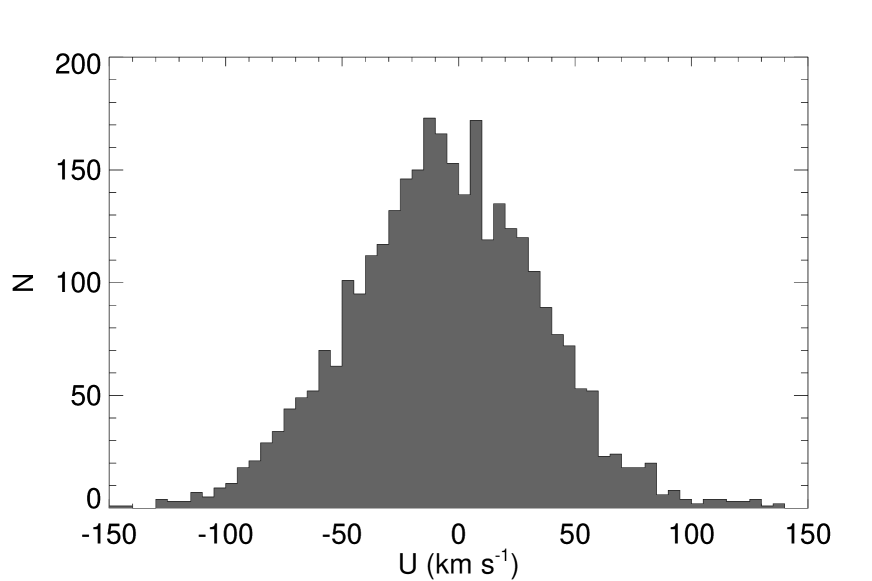
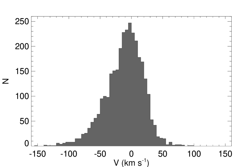
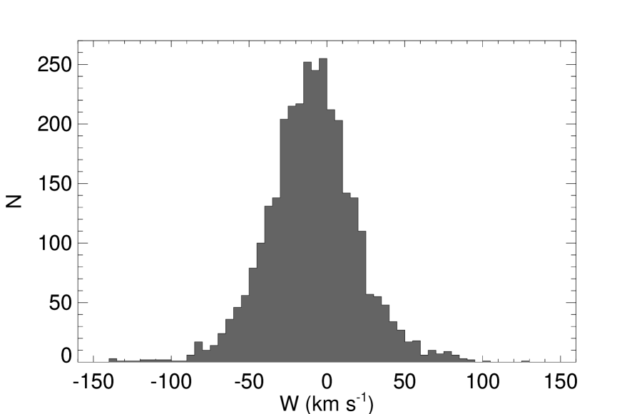
Figure 12: Distributions of the space velocities $(U,\,V,\,W)$ for those white dwarfs with spectra with SNR$>$20, $M_{\rm WD}>0.45\,M_{\sun}$ and $\Delta U,\,\Delta V,\Delta W<35$ km s^-1. The distribution of the $V$ component shows a long tail towards negative values, a consequence of the asymmetric drift. These stars lag behind the LSR.

Finally, we also estimated the Galactocentric distances $R_{\rm G}$ of each white dwarf in our sample. This was done using their distances $d$, and Galactic coordinates $(l,b)$ (see Fig.1). Adopting a Sun Galactocentric distance, $R_{\sun}=8.34\pm 0.16\,$kpc (Reid et al., 2014), we found that most white dwarfs in this study are located between $7.8<R_{\rm G}<9.3\,$kpc. In the following sections, we will use $R_{\rm G}$ together with $Z$ to investigate the velocity distributions.

3.6 Proper motions

We obtained proper motions and their associated uncertainties for the objects of our sample using the casjobs interface (Li & Thakar, 2008), which combines SDSS and re-calibrated USNO-B astrometry (Munn et al., 2004, 2014). These proper motions are calculated from the USNO-B1.0 plate positions re-calibrated using nearby galaxies together with the SDSS position so that the proper motions are more accurate and absolute. By measuring the proper motions of quasars, Munn et al. (2004, 2014) estimate that 1$\sigma$ error is $\sim 4\,$mas yr^-1. In Fig. 11 we compare the measurement of the proper motion, in right ascension, and declination for 125 objects in common in our white dwarf data-set between SDSS-USNO-B (Munn et al., 2014) and UCAC4 catalogue (Zacharias et al., 2013). We found a good agreement between both measurements for most of the common objects. Unfortunately, for 4,360 DA white dwarfs in our sample there are no available proper motions.

3.7 Space velocities

Figure 13: $U-V$, $U-W$, and $V-W$ diagrams for the selected sample of white dwarfs.

We computed the velocities in a cartesian Galactic system following the method developed by Johnson & Soderblom (1987). That is, we derived the space velocity components $(U,\,V,\,W)$ from the observed radial velocities, proper motions and distances. We considered a right-handed Galactic reference system, with $U$ positive towards the anticenter, $V$ in the direction of rotation, and $W$ positive towards the North Galactic Pole (NGP). The uncertainties in the velocity components $U$, $V$ and $W$ were derived using the formalism of Johnson & Soderblom (1987). Within this framework the equation for the variance of a function of several variables is used. Johnson & Soderblom (1987) assumed that the matrix used to transform coordinates into velocities introduces no error in $U$, $V$ or $W$. Consequently, the only sources of error are the distances, proper motions and radial velocities. Furthermore, this method assumes that the errors of the measured quantities are uncorrelated, i.e. that the covariances are zero. We found that the typical error is ($\Delta U,\,\Delta V,\,\Delta W$) $\sim(6.5,\,8.3,\,10.5)\,$km s^-1 and that nearly the entire sample has $\Delta U,\,\Delta V,\Delta W<35\,$km s^-1.

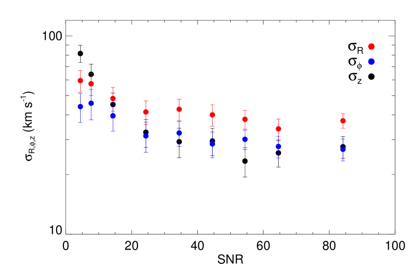
Figure 14: Distribution of the velocity dispersion as a function of the SNR. The velocity dispersion for white dwarfs with spectra with SNR$<$20 is dominated by random errors while for stars with spectra with SNR$>$20 the average value of the velocity dispersion of the three velocity components remains constant independently of the uncertainties, suggesting a physical origin.

Fig. 12 shows the $U$, $V$ and $W$ distributions for the SDSS DA white dwarfs. Only white dwarfs with $M_{\rm WD}>0.45\,M_{\sun}$ — to avoid contamination from close binaries, see Sect. 3.2 — and spectra with SNR$>$20 — to ensure a RV error smaller than 20 km $s^{-1}$, see Sect. 3.4 — and reasonable uncertainties $\Delta U,\,\Delta V$, and $\Delta W<35$ km s^-1 were selected. Also, in Fig. 13 we show the phase-space diagrams for the same sample. These diagrams reveal interesting substructure in the Galactic disc, i.e. moving groups in the $U$-$V$ plane (Nordström et al., 2004). A detailed study of the overdensities and outliers objects seen in the phase-space using a population synthesis code (Torres et al., 2002) is underway.

Since white dwarfs in our sample are located at relatively large distances from the Sun, we also use cylindrical coordinates, with $V_{\rm R}$, $V_{\rm\phi}$ and $V_{\rm z}$ defined as positive with increasing $R_{\rm G}$, $\phi$ and $Z$, with the latter towards the NGP. We took the motion of the Sun with respect to the Local Standard of Rest (LSR) (Schönrich et al., 2010), that is ($U_{\sun},\,V_{\sun},\,W_{\sun})=(-11,\,+12,\,+7)\,$km s^-1. The LSR was assumed to be on a circular orbit, with circular velocity $\Theta=240\pm 8$ km s^-1 (Reid et al., 2014). With these values we computed the cylindrical velocities of our sample, $V_{\rm R}$, positive towards the Galactic center, in consonance with the usual $U$ velocity component, $V_{\rm\phi}$, towards the direction of rotation and $V_{\rm z}=W$, positive towards the NGP – see appendix in Williams et al. (2013) for more details.

To compute the uncertainties of the velocities in the cylindrical coordinate system we cannot assume that the observables are uncorrelated. To propagate the non-independent random errors in the velocities in this coordinate frame we used a Monte Carlo technique that takes into account the uncertainties in the distances ($\Delta X,\,\Delta Y,\,\Delta Z$) and in the space velocities in cartesian coordinates ($\Delta U,\,\Delta V,\,\Delta W$). This Monte Carlo algorithm for error propagation allows to easily track the error covariances. In essence, we generated a distribution of 1,000 test particles around each input value of $(XYZ,\,UVW)$, assuming Gaussian errors with standard deviations given by the formal errors in the measurements for each white dwarf, and then we calculate the resulting ($V_{\rm R}$, $V_{\rm\phi}$, $V_{\rm z}$) and their corresponding 1$\sigma$ associated uncertainties.

4 Velocity maps and age gradients

In the previous sections we have introduced our SDSS DA white dwarf sample and we have explained how we have derived the stellar parameters, ages, distances, radial velocities and proper motions for each star. With this information at hands we analyze the kinematic properties of the observed sample. This is fully justified because our sample of DA white dwarfs culled from the SDSS DR 12 catalog is statistically significant, independently of the restrictions applied to the full sample to use only high-quality data. These restrictions are explained below, and quite naturally, reduce the total number of white dwarfs. Finally, we emphasize that a thorough analysis of the effects of the selection procedures and observational biases using a detailed population synthesis code (García-Berro et al., 1999; Torres et al., 2002; García-Berro et al., 2004) is underway, and we refer the reader to a forthcoming publication.

Table 3: Average values for the Galactic cylindrical velocities $(V_{\rm R},\,V_{\rm\phi},\,V_{\rm z})$ and their corresponding dispersions as a function of the Galactocentric distance $R_{\rm G}$.

$R_{\rm G}$ (kpc)	$\langle V_{\rm R}\rangle$ (km s-1)	$\sigma_{\rm R}$ (km s-1)	$\langle V_{\rm\phi}\rangle$ (km s-1)	$\sigma_{\rm\phi}$ (km s-1)	$\langle V_{\rm z}\rangle$ (km s-1)	$\sigma_{\rm z}$ (km s-1)
$<$ 7.90	+11.3 $\pm$ 5.2	31.1 $\pm$ 6.1	+215.2 $\pm$ 5.3	25.7 $\pm$ 5.3	+8.9 $\pm$ 4.3	33.9 $\pm$ 6.5
7.90 – 8.15	+2.5 $\pm$ 1.0	35.9 $\pm$ 2.2	+232.9 $\pm$ 0.9	26.5 $\pm$ 1.7	–5.1 $\pm$ 0.9	24.5 $\pm$ 1.5
8.15 – 8.40	+2.1 $\pm$ 0.2	26.1 $\pm$ 0.6	+224.6 $\pm$ 0.2	21.5 $\pm$ 0.5	–10.2 $\pm$ 0.2	23.7 $\pm$ 0.4
8.40 – 8.65	+14.2 $\pm$ 0.3	33.7 $\pm$ 0.8	+233.5 $\pm$ 0.3	22.7 $\pm$ 0.6	–10.5 $\pm$ 0.2	27.1 $\pm$ 0.6
8.65 – 8.85	+5.4 $\pm$ 0.9	34.1 $\pm$ 2.1	+236.4 $\pm$ 0.9	23.5 $\pm$ 1.4	–2.9 $\pm$ 0.9	16.4 $\pm$ 1.2
$>$ 8.85	+3.4 $\pm$ 2.8	36.0 $\pm$ 4.3	+237.3 $\pm$ 2.7	22.1 $\pm$ 2.8	–2.7 $\pm$ 2.9	21.5 $\pm$ 2.9

Table 4: Average values for the Galactic cylindrical velocities $(V_{\rm R},\,V_{\rm\phi},\,V_{\rm z})$ and their corresponding dispersions as a function of the Galactic height $Z$.

$Z$ (kpc)	$\langle V_{\rm R}\rangle$ (km s-1)	$\sigma_{\rm R}$ (km s-1)	$\langle V_{\rm\phi}\rangle$ (km s-1)	$\sigma_{\rm\phi}$ (km s-1)	$\langle V_{\rm z}$ $\rangle$ (km s-1)	$\sigma_{\rm z}$ (km s-1)
$<-0.5$	+4.8 $\pm$ 4.8	42.0 $\pm$ 7.9	+212.7 $\pm$ 4.8	23.9 $\pm$ 4.9	+13.0 $\pm$ 4.5	27.8 $\pm$ 5.5
$-0.50$ – $-0.25$	+17.0 $\pm$ 1.2	37.1 $\pm$ 2.8	+226.9 $\pm$ 1.1	31.9 $\pm$ 2.3	+7.3 $\pm$ 1.3	23.4 $\pm$ 1.9
$-0.25$ – 0.00	+11.1 $\pm$ 0.3	32.4 $\pm$ 1.2	+226.6 $\pm$ 0.3	24.7 $\pm$ 0.9	+10.6 $\pm$ 0.3	20.8 $\pm$ 0.9
0.00 – +0.25	+2.1 $\pm$ 0.1	27.2 $\pm$ 0.6	+225.7 $\pm$ 0.1	21.6 $\pm$ 0.4	–14.0 $\pm$ 0.2	21.9 $\pm$ 0.4
+0.25 – +0.50	+5.4 $\pm$ 0.4	34.4 $\pm$ 1.0	+235.3 $\pm$ 0.4	23.7 $\pm$ 0.7	–9.5 $\pm$ 0.4	24.4 $\pm$ 0.7
$>$ +0.50	+4.9 $\pm$ 1.8	37.6 $\pm$ 2.9	+237.8 $\pm$ 1.9	24.7 $\pm$ 2.1	–2.6 $\pm$ 1.8	29.5 $\pm$ 2.4

As mentioned, the catalog used in this work contains 20,247 DA white dwarfs culled from the SDSS DR 12. To study the behavior of the velocity components with respect to the Galactocentric distance ($R_{\rm G}$) and to the vertical distance ($Z$) we restricted our sample to employ only stars with data of the highest quality. First of all, we explored the effects of selecting stars with spectra with qualities above a given SNR threshold. We found that both the resulting velocity dispersions and the average velocities are sensitive to this choice. Hence, a natural question arises, namely what is the optimal SNR cut to achieve our science goals without discarding an excessive number of stars. To address this question in Fig. 14 we examine the behavior of the velocity dispersion as a function of the SNR cut. The error bars are the standard deviation of the uncertainties in the velocities for the corresponding SNR bin. Note that for white dwarfs with spectra with SNR$<$20 random errors dominate the velocity dispersion, while for stars with spectra with SNR$>$20 the dispersion remains constant within the error bars, suggesting that a physical dispersion, which is not due to the uncertainties in the observables, exists. Hence, we only selected stars with spectra having SNR$>$20. We also excluded from this sub-sample all white dwarfs with masses below $0.45\,M_{\sun}$. In this way we avoid an undesirable contamination by close binaries — see the discussion in Sect. 3.2. Furthermore, we only considered white dwarfs with reasonable determinations, and consequently we excluded those stars for which the velocity errors were large — see Sect. 3.7. In particular, we adopted a cut $\Delta_{U,V,W}<35\,$km s^-1. We also did not consider those white dwarfs with velocities $-600\,<\,V_{\rm R},V_{\rm\phi},V_{\rm z}\,<\,600$ km s^-1 to remove outliers. This resulted in a sub-sample of 3,415 DA white dwarfs. Since the aim of this section is to gain a preliminary insight on the general behavior of the velocities and velocity dispersions, we do not distinguish between halo, thick and thin disc white dwarfs.

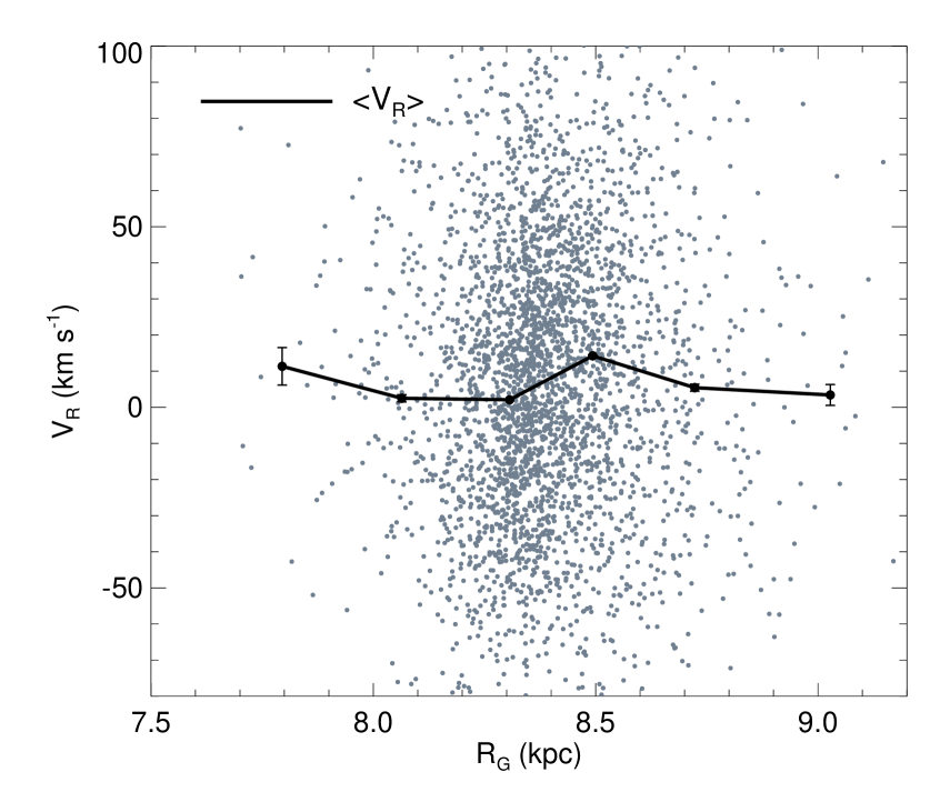
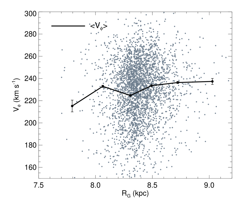
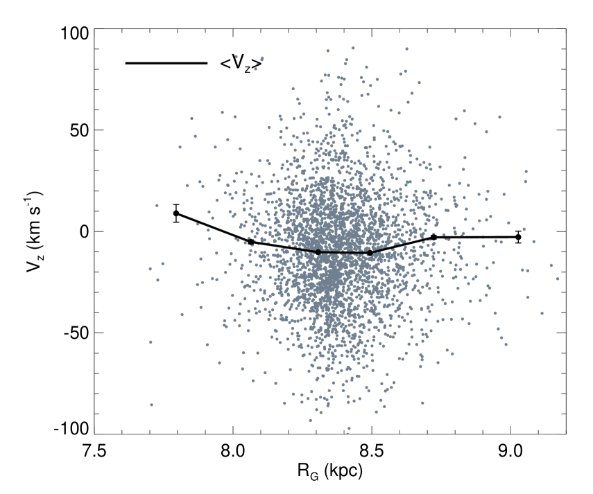
Figure 15: Average velocities as a function of $R_{\rm G}$. See text for more details.

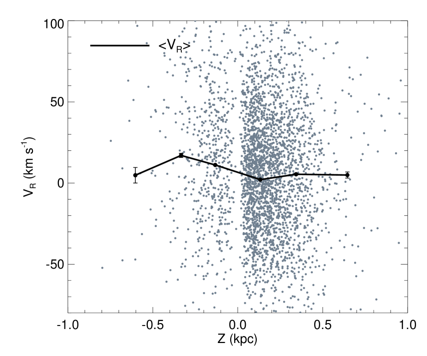
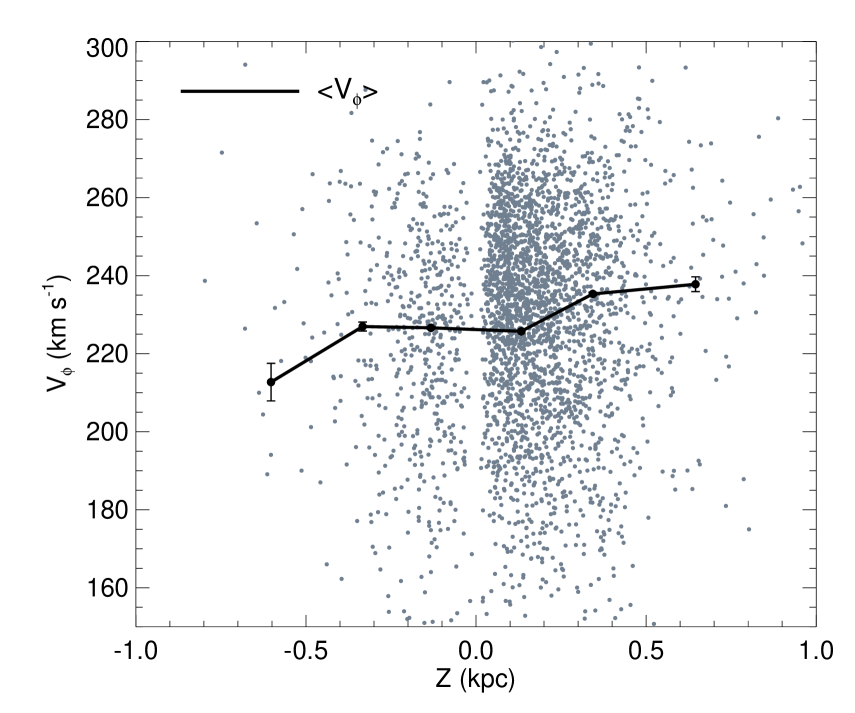
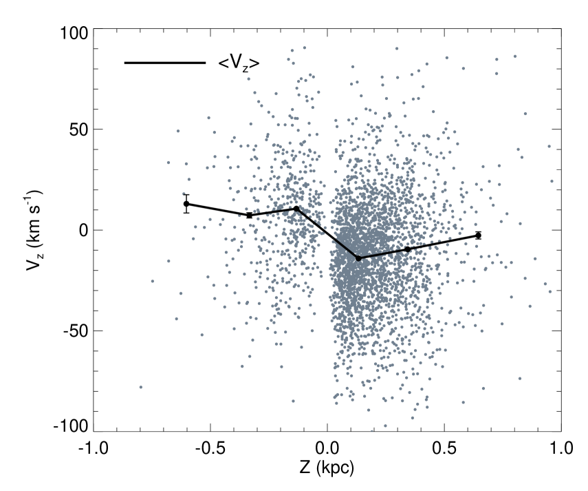
Figure 16: Average velocities as a function of $Z$. See text for more details.

This sub-sample allowed us to study the behavior of the components of the velocity as a function of the Galactocentric distance ($R_{\rm G}$) and the vertical distance ($Z$). We used weighted means and weighted velocity dispersions. The expression for the weighted mean of any (say $\omega$) of the three components of the velocities is:

$$\langle V_{\omega}\rangle=\frac{\displaystyle\sum_{i=1}^{N}\eta_{i}V_{\omega_{i}}}{\displaystyle\sum_{i=1}^{N}\eta_{i}}$$ (1)

where $V_{\omega_{i}}$ is the $\omega$ component of the velocity for each star. In this expression the weights are given by $\eta_{i}=1/\sigma^{2}_{\omega_{i}}$, being $\sigma_{\omega_{i}}$ the error associated to the three components of the velocity ($\Delta V_{\rm R},\,\Delta V_{\rm\phi},\,\Delta V_{\rm z}$) of each individual white dwarf. The variance of $\langle V_{\omega}\rangle$ is given by:

$$\sigma_{\omega}^{2}=\frac{1}{\displaystyle\sum_{i=1}^{N}1/\sigma_{\omega_{i}}^{2}}$$ (2)

To compute the velocity dispersion of the stellar velocity components we used a weighted variance:

$$\sigma_{V_{\omega}}^{2}=\frac{\displaystyle\sum_{i=1}^{N}\eta_{i}(V_{\omega_{i}}-\langle V_{\omega}\rangle)^{2}}{k\displaystyle\sum_{i=1}^{N}\eta_{i}}$$ (3)

where $k=(N^{\prime}-1)/N^{\prime}$, and $N^{\prime}$ is the number of non-zero weights. The error bars of the velocity dispersion in Figs. 15 and 16 weere computed employing the expression

$$\Delta{V_{\omega}}=(2N)^{-1/2}\sigma_{V_{\omega}}$$ (4)

where $N$ is the number of white dwarfs in each bin of $R_{\rm G}$ and $Z$ respectively (see also Table 3 and Table 4), used to calculate $\sigma_{V_{\omega}}$.

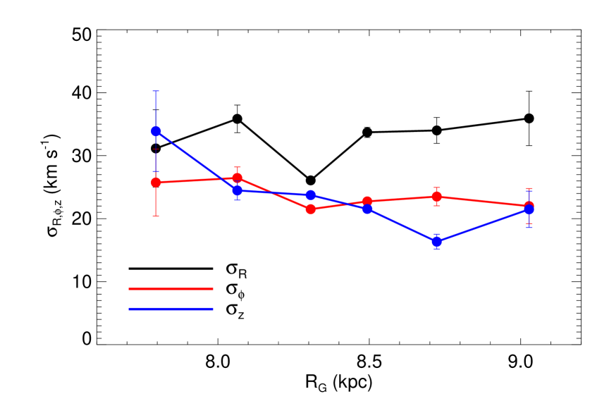
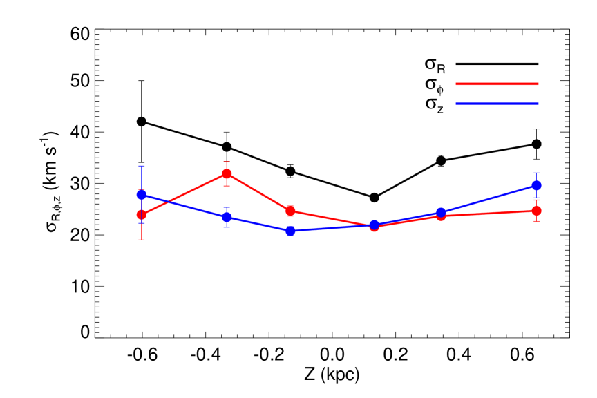
Figure 17: Left panel: variation of the velocity dispersion for the three velocity components with respect to the Galactocentric distance. Right panel: variation of the velocity dispersion with respect to the vertical Galactic distance $Z$.

4.1 Space velocities in the local volume

In Figs. 15 and 16 we show the three components of the space velocity $(V_{\rm R},\,V_{\rm\phi},\,V_{\rm z})$ for each white dwarf in this sub-sample as a function of $R_{\rm G}$ and $Z$, respectively. We also show the average (black lines). In Fig. 17 we show the velocity dispersion as a function of $R_{\rm G}$ and $Z$. The velocity dispersion components are corrected for the measuring errors using the standard deviation of the error distribution per each bin. Most white dwarfs in this sub-sample with precise kinematics are close to the Galactic plane, with altitudes from the Galactic plane within $\pm 0.5\,$kpc. Also, the vast majority of these stars are located at Galactic radii ranging from $R_{\rm G}=8.0$ kpc to 8.8 kpc. In the local volume covered by our sample we found that the average value of the radial velocity $V_{\rm R}$ first slightly increases for increasing distances from the center of the Galaxy, and then decreases up to $R_{\rm G}\simeq 8.5$ kpc. From this point outwards the average velocity remains nearly constant. The radial velocity dispersion $\sigma_{\rm R}$ slightly increases as $R_{\rm G}$ increases (see Table 3). For white dwarfs around $R_{\rm G}\sim 8.0\,$kpc we found $V_{\rm R}\sim+2.5\pm 1.0\,$km s^-1, while for $R_{\rm G}\sim 9.0\,$kpc we have $V_{\rm R}\sim+3.4\pm 2.8\,$km s^-1. However, at larger distances, for example, $R_{\rm G}<7.9$ kpc and $Z<-0.5\,$kpc, Poisson noise contributes significantly. This noise is beyond the formal measurement errors of the measured kinematic properties as these bins contain only a few white dwarfs (note that Poisson noise scales as $N^{-1/2}$, where $N$ is the number of objects in the bin).

Siebert et al. (2011) and Williams et al. (2013), using a sample of red clump stars from the RAVE survey that covers a volume larger than that probed by our sample of white dwarfs; also reported a radial gradient in the mean Galactocentric radial velocity, $V_{\rm R}$. In particular, if we restrict ourselves to stars with altitudes $-0.5<Z<0.5\,$kpc we find a small negative gradient $\partial\langle V_{\rm R}\rangle/\partial R_{\rm G}=-3\pm 5\,$km s^-1 kpc^-1 while the gradient of the velocity dispersion is $\partial\sigma_{\rm R}/\partial R_{\rm G}=+3\pm 4\,$ km s^-1 kpc^-1. Interestingly, $V_{\rm R}$ shows a small gradient in the vertical direction, $\partial\langle V_{\rm R}\rangle/\partial Z=-5\pm 6\,$km s^-1 kpc^-1. However, the errors are too large to draw any robust conclusion. For the variation of $\sigma_{\rm R}$ with respect to the vertical distance we found the following, $\partial\sigma_{\rm R}/\partial Z=-23\pm 5\,$km s^-1 kpc^-1 for for Z $<$ 0, suggesting a substantial gradient while $\partial\sigma_{\rm R}/\partial Z=+19\pm 3\,$km s^-1 kpc^-1 for Z $>$ 0. $\sigma_{\rm R}$ clearly increases when moving away from the Galactic plane (see Table. 4).

As well known from the Jeans equation $V_{\rm\phi}$ decreases as the asymmetric drift increases, and hence when $\sigma_{\rm\phi}$ increases (Binney & Tremaine, 2008). We found a positive gradient with respect to $R_{\rm G}$, $\partial\langle V_{\rm\phi}\rangle/\partial R_{\rm G}=+15\pm 5\,$km s^-1 kpc^-1. Moving inwards, $V_{\phi}$ decreases. For the velocity dispersion we found a negative gradient in terms of $R_{\rm G}$, $\partial\sigma_{\rm\phi}/\partial R_{\rm G}=-3\pm 1\,$km s^-1 kpc^-1, the velocity dispersion increases when moving inwards. Also, it is interesting to investigate the profile of $V_{\rm\phi}$ with respect to the vertical height. Our data allows us to detect a significant gradient, $\partial\langle V_{\rm\phi}\rangle/\partial Z=+17\pm 4\,$km s^-1 kpc^-1, suggesting that the outer region of the South Galactic Pole, rotates slower than those regions close to the North. However, as mentioned above, the number of white dwarfs with $Z<-0.5\,$kpc is small, and Poisson noise, among other selection biases, may play a role. The velocity dispersion, $\sigma_{\rm\phi}$ also shows a small gradient. For Z $<$ 0, we have $\partial\sigma_{\rm\phi}/\partial Z=+3\pm 18\,$km s^-1 kpc^-1 while for Z $>$ 0, $\partial\sigma_{\rm\phi}/\partial Z=+6\pm 2\,$km s^-1 kpc^-1. We also found that $\sigma_{\rm\phi}$ increases ($\Delta\sigma_{\rm\phi}\sim$ 4 km s^-1) when $\lvert Z\rvert$ increases from zero to $0.6\,$kpc, reaching a minimum value of $\sigma_{\rm\phi}=+21.6\pm 0.4\,$km s^-1 at $0<Z<+0.25\,$kpc.

Figs. 15, 16, 17 also shows how the mean value of $V_{\rm z}$ and $\sigma_{\rm z}$ behave with respect to $R_{\rm G}$ and $Z$. A small gradient is found, $\partial V_{\rm z}/\partial R_{\rm G}=-6\pm 7\,$km s^-1 kpc^-1, suggesting that for this range of values of $Z$ the mean vertical velocity increases when $R_{\rm G}$ decreases. The vertical velocity dispersion, $\sigma_{\rm z}$, clearly decreases when moving away from the Galactic center, the gradient being $\partial\sigma_{z}/\partial R_{\rm G}=-10\pm 4\,$km s^-1 kpc^-1. The profile of the mean value of $V_{z}$ as a function of the vertical distance, $Z$, also shows an interesting trend. Specifically, while for white dwarfs with positive $Z$ (in the North Galactic hemisphere) we have negative values in $\langle V_{\rm z}\rangle$, for white dwarfs with $Z<0$ (in the South Galactic hemisphere), $\langle V_{\rm z}\rangle$ is positive. Our dataset shows a gradient $\partial V_{\rm z}/\partial Z=-18\pm 8\,$km s^-1 kpc^-1. We also found that the velocity dispersions increase when moving away from the Galactic plane, $\Delta\sigma_{\rm z}\sim 10\,$km s^-1 from the Galactic plane to $0.6\,$kpc with a significant gradient, $\partial\sigma_{\rm z}/\partial Z=-15\pm 1\,$km s^-1 kpc^-1 for Z $<$ 0 and $\partial\sigma_{\rm z}/\partial Z=+15\pm 2\,$km s^-1 kpc^-1 for Z $>$ 0. We note that the variation of $\sigma_{\rm z}$ with $Z$ has received significant attention as it can be used to trace the vertical potential of the disc (Smith et al., 2012).

For the local sample of white dwarfs used in this study we found that the inner part of the Galaxy is hotter than the outer part, $\sigma_{\rm R,\phi,z}(R_{\rm G}<R_{\sun})>\sigma_{\rm R,\phi,z}(R_{\rm G}>R_{\sun})$. The radial gradient in the velocity dispersion is well known and also detected in other galaxies, e.g. van der Kruit & Freeman (2011). We also found that the velocity dispersions increase when moving away from the Galactic plane, $\sigma_{\rm R,\phi,z}$ ($\lvert Z\rvert=0)<\sigma_{\rm R,\phi,Z}$ ($\lvert Z\rvert$ $>$ 0). Figs. 15, 16, 17 and Tables 3 and 4 summarize the results discussed here.

4.2 Radial and vertical age gradients

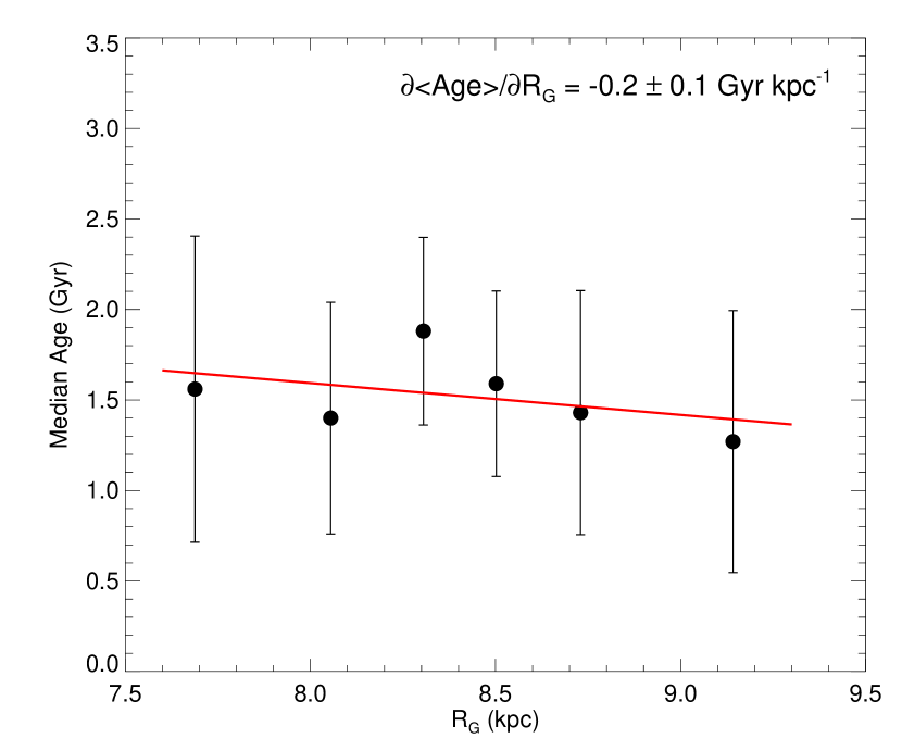
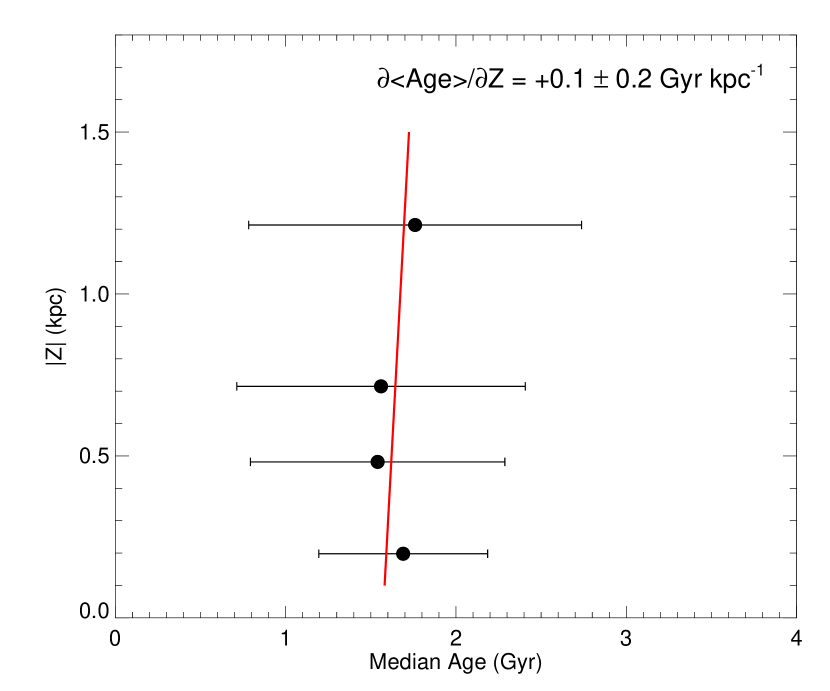
Figure 18: Median age as a function of the Galactocentric distance $R_{\rm G}$ (left panel) and vertical distance $Z$ (right panel).

In this section we study the radial and vertical age gradients on the Milky Way disc using the derived white dwarf ages. West et al. (2011) reported variations in the fraction of active M dwarfs of similar spectral type at increasing Galactic latitudes as an indirect evidence for the existence of a vertical age gradient in the Milky Way disc. Recently, Casagrande et al. (2016) using red giants and seismic ages by Kepler mission reported that old red giants dominate at increasing Galactic heights. They also reported a vertical gradient of approximately 4 Gyr kpc^-1, although with a large dispersion of ages at all heights and considerably large uncertainties, that prevented them to derive meaningful conclusions.

Note that, as mentioned before, our data-set contains white dwarfs with ages $<4.5$ Gyr. Hence, intermediate-old stars are missing in this study and this may introduce a bias in our results. By selecting intervals in $R_{\rm G}$ and $\lvert Z\rvert$ we estimated the median age. For stars within this bin we also computed the mean values of $R_{\rm G}$ and $\lvert Z\rvert$. Then, we used a linear regression to compute the age gradients as well as their correspond $1\sigma$ uncertainties. In Fig. 18 the median stellar age as a function of Galactocentric distance $R_{\rm G}$ (left panel) and height $\lvert Z\rvert$ (right panel) for $7.6<R_{\rm G}<9.2\,$kpc and $0.1<\lvert Z\rvert<1.3\,$kpc are displayed, together with the resulting linear fit (red line). The error bars in any given bin were computed as $\Delta_{\tau}=(2N)^{-1/2}\sigma_{\tau}$, where $N$ is the number of white dwarfs in each bin. We found a very small negative radial and positive vertical age gradients, $\partial\langle\tau\rangle/\partial R_{\rm G}=-0.2\pm 0.1\,$Gyr kpc^-1 and $\partial\langle\tau\rangle/\partial Z=+0.1\pm 0.2\,$Gyr kpc^-1, respectively. However, these results together with their associated uncertainties are also compatible with zero radial and vertical gradients for the volume probed in our study.

Figure 19: Age-velocity relation for the three components of the stellar velocity, $V_{\rm R}$, $V_{\rm\phi}$, and $V_{\rm z}$, the IFMR of Catalán et al. (2008) is used to estimate the ages of the white dwarfs. Our sample is limited to stars younger than 4.5 Gyr.

5 The age-velocity relation

In this section we explore the age-velocity and the age-velocity dispersion relationships of the Galactic disc. We restricted our sample, as discussed in Sect. 4, to those stars with the highest quality data. Our final sample contains 3,415 DA white dwarfs for which the typical age uncertainty is $\leq 0.5$ Gyr. Fig. 19 shows the three components of the velocity in cylindrical coordinates ($V_{\rm R},\,V_{\rm\phi},\,V_{\rm z}$) as a function of age when the IFMR of Catalán et al. (2008) is used. Unfortunately, when this IFMR is used our sample does not contain stars older than 4.0 Gyr, and the same occurs when the relationships of Ferrario et al. (2005) and Gesicki et al. (2014) are employed. This is due to the tight quality requirements we have introduced. Hence, we are restricted to the study of the latest few Gyr of evolution from the formation of the Milky Way disc.

Figure 20: Toomre diagram for our white dwarf sample. The $V$ component of the stellar velocity represents the stellar angular momentum and has an asymmetric distribution as discussed in Fig. 12, while the combination of $U$ and $W$ is a measure of the orbital energy. Dotted lines show curves of constant speed, i.e., the curves for which $U^{2}+V^{2}+W^{2}$ remains constant.

5.1 Thin, thick disc and halo sample

There is observational evidence that a sizable fraction of the thick disc is chemically different from the dominant thin disc. Studies of abundance populations based on high resolution spectroscopy find that the abundance distribution is bimodal — see , e.g., Navarro et al. (2011), Fuhrmann (2011), and Bensby et al. (2014). This strongly suggests that the thin and thick disc have a different physical origin. Moreover, most of the thick Galactic disc population is kinematically hotter than that of the thin disc (Freeman, 2012). However, the strong gravities of white dwarfs do not allow to use the metallicity to classify white dwarfs, because all metals are diffused inwards in short timescales, resulting in atmospheres made of pristine hydrogen. Thus, to study the membership of white dwarfs in our sample to the thick or to the thin disc we rely exclusively on their kinematical properties. In view of this, a Toomre diagram is useful to understand the characteristics of final DA white dwarf sample. This diagram combines vertical and radial kinetic energies as a function of the rotational energy. Several studies based in the analysis of the abundances of the Galactic populations — e.g., Nissen (2004) and Bensby et al. (2014) — have concluded that to a first approximation low-velocity stars (that is, those with $V_{\rm tot}<70\,$km s^-1) mainly belong to the thin disc, whereas stars with $V_{\rm tot}>70\,$km s^-1 but with velocities smaller than $\sim$ 200 kms^-1, are likely to belong to the thick disc. However, the velocity cutoff selection population strongly depends on the size of the sample. Moreover, a pure kinematical selection of thin/thick disc stars can introduce a severe bias in our studies, as observed by different authors where subpopulations were selected using individual chemical abundances (Adibekyan et al., 2013; Bensby et al., 2014).

According to this, from Fig. 20 it follows that our sample is dominated by thin disc white dwarfs, although certainly some stars in the sample exhibit thick disc kinematics. Moreover, Fig. 17 shows that the $\sigma_{\rm z}$ velocity dispersion rises with $\lvert Z\rvert$, which could be at least partly due to a component hotter than the thin disc. In order to study the fraction of thin, thick and halo stars in our WD sample, we performed a gaussian mixture model on their V_z distribution, to see if the velocity distribution shows multiple components. The model uses maximum likelihood to get the parameters for gaussian components, and takes account of the measuring errors for the velocities of individual stars. We find that the z-velocity distribution is dominated by a single colder component, with a velocity dispersion of about 23 $\pm$ 0.5 km s^-1 and showing no significant change with age. A weak hotter component is also seen, containing about 5$\%$ of the total sample (about 100 stars), with a velocity dispersion of 72 $\pm$ 6 km s^-1, again showing no significant change with age.

We can compare the dispersion of the colder component of the white dwarfs (23 km s^-1) with the AVR from the Casagrande et al. (2011) sample of Geneva-Copenhagen Survey (GCS) stars. This is probably the best source of age-velocity data available for nearby stars. The GCS stars have isochrone ages and are mostly turnoff stars. Fig. 23 shows the AVR for GCS stars with [Fe/H] $>$ -0.3; this cut removes most of the thick disc stars from the sample. The GCS stars show a well defined AVR, with the $\sigma_{\rm z}$ velocity dispersion rising with age from about 10 km s^-1 for the youngest stars, and levelling out at about 23 km s^-1 for stars older than about 5 Gyr. We note that the 23 km s^-1 dispersion of the colder component of the white dwarfs (ages mostly $<$ 4 Gyr) is in excellent agreement with the dispersion of the older thin disc stars in Fig 23. The velocity dispersion of the weak hotter component from the mixture model is about 72 km s^-1. This is much larger than the typical z-velocity dispersion of thick disc stars near the sun (about 40 km s^-1), and suggests that there may also be a few halo WDs in the sample. However, in this we will not attempt to fully analyze and characterize each kinematic component of our sample. Thus, we do not apply any a priori kinematical cut to distinguish between thin and thick stars to study the AVR.

5.2 The age-velocity dispersion relation

The age-velocity dispersion relation is a fundamental relation to understand local Galactic dynamics. It reflects the slow increase of the random velocities with age due to the heating of the stellar disc. We study this relation using the ages estimated using the three IFMRs discussed in Sect. 3.3. To this end, we first binned the data in intervals of 1 Gyr, and then we computed the stellar velocity dispersions and their associated errors following the expressions discussed in Sect. 4. The velocity dispersion components were also corrected for the measuring errors using the standard deviation of the error distribution for each age bin.

Table 5: Velocity dispersions as a function of the age for the three IFMRs studied in this work.

Age (Gyr)	$\sigma_{\rm R}$ (km s-1)	$\sigma_{\rm\phi}$ (km s-1)	$\sigma_{\rm z}$ (km s-1)
	Catalán et al. (2008)
0 – 1	24.6 $\pm$ 0.8	17.7 $\pm$ 0.6	19.8 $\pm$ 0.6
1 – 2	24.6 $\pm$ 0.6	19.2 $\pm$ 0.4	22.6 $\pm$ 0.5
2 – 3	28.9 $\pm$ 0.9	21.8 $\pm$ 0.7	23.5 $\pm$ 0.7
3 – 4	30.3 $\pm$ 1.2	22.5 $\pm$ 0.9	21.4 $\pm$ 0.8
4 – 5	31.1 $\pm$ 2.0	26.9 $\pm$ 1.7	21.8 $\pm$ 1.4
	Ferrario et al. (2005)
0 – 1	24.5 $\pm$ 0.6	17.9 $\pm$ 0.5	19.5 $\pm$ 0.5
1 – 2	27.0 $\pm$ 0.6	20.5 $\pm$ 0.4	22.1 $\pm$ 0.5
2 – 3	27.1 $\pm$ 1.0	21.8 $\pm$ 0.8	25.8 $\pm$ 1.0
3 – 4	32.3 $\pm$ 2.0	25.9 $\pm$ 1.6	22.9 $\pm$ 1.4
	Gesicki et al. (2014)
0 – 1	24.0 $\pm$ 0.7	17.5 $\pm$ 0.5	19.4 $\pm$ 0.6
1 – 2	27.2 $\pm$ 0.5	20.5 $\pm$ 0.4	21.9 $\pm$ 0.4
2 – 3	26.9 $\pm$ 1.0	22.8 $\pm$ 0.8	25.1 $\pm$ 1.0
3 – 4	37.3 $\pm$ 3.6	24.2 $\pm$ 2.3	24.8 $\pm$ 2.4

Our results indicate that the three components of the stellar velocity dispersion increase with time, independently of the adopted IFMR. This is illustrated in Fig. 21 — see also Table 5. When we use the IFMR of Catalán et al. (2008) for stars older than 2.5 Gyr $\sigma_{\rm\phi}$ increases with time, while $\sigma_{\rm R}$ remains nearly constant within the errors, and $\sigma_{\rm Z}$ remains also constant. However, it should be taken into account that the number of stars older than 3.5 Gyr is small for all three IFMRs, although the number of stars older than 3.5 Gyr is significantly larger for the IFMR of Catalán et al. (2008). Thus, only in this case the age-velocity dispersion relation for ages longer than 4 Gyr, but still shorter than 5.5 Gyr can be explored. For the rest of the IFMRs the results are less significant. Nevertheless, it is interesting to realize that, as it occurs for the IFMR of Catalán et al. (2008), for both the IFMRs of Ferrario et al. (2005) and Gesicki et al. (2014) all three components of the stellar velocity dispersion increase for ages smaller than $\sim 2.5\,$Gyr, while for ages larger than this $\sigma_{\rm R}$ and $\sigma_{\rm\phi}$ increases both cases, while $\sigma_{\rm z}$ saturates.

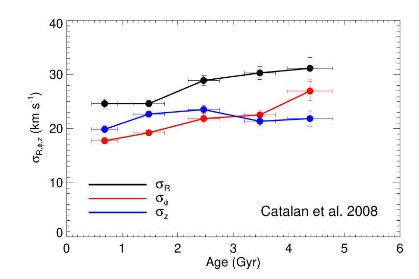
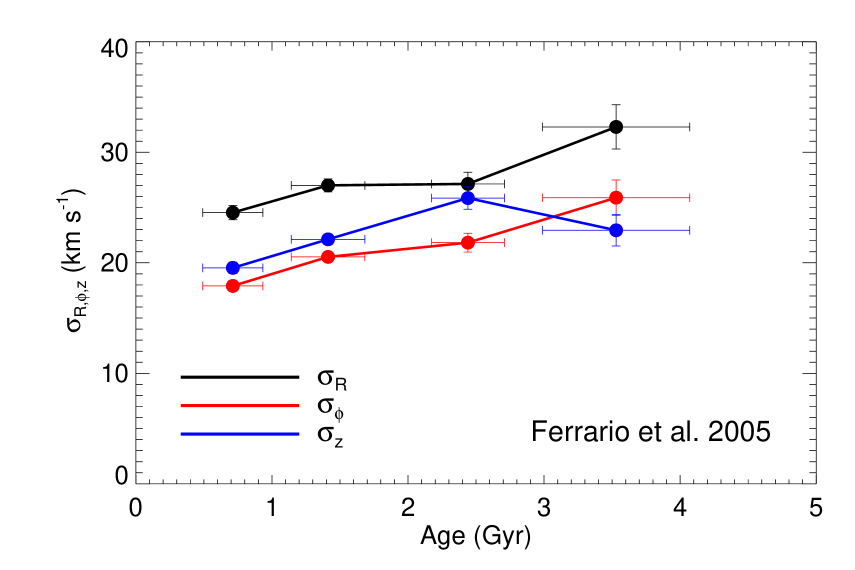
Figure 21: Age-velocity dispersion relation for a total of 2,345 DA white dwarfs binned in 1 Gyr intervals. The top panel shows the results using the ages obtained using the IFMR of Catalán et al. (2008), the middle panel shows the ages derived using the IFMR of Ferrario et al. (2005), whereas for the bottom panel the IFMR of Gesicki et al. (2014) was adopted. The corresponding dispersions, $\sigma_{\rm R}$, $\sigma_{\rm\phi}$ and $\sigma_{\rm z}$ are shown in red, blue and black, respectively.

Age-velocity dispersion relations are suitable to constrain heating mechanisms taking place in the Galactic disc during the first epochs. Since dynamical streams are well mixed in the vertical direction (Seabroke & Gilmore, 2007) we will use the age-$\sigma_{\rm z}$ relation. The vertical velocity dispersion obtained when the ages derived employing the semi-empirical IFMR of Catalán et al. (2008), together with the associated uncertainties, is displayed in Fig. 22 using black dots. In this figure we also show two dynamical heating functions following a power law as a function of the age ($\tau$), $\sigma_{\rm z}\propto\tau^{\alpha}$, with $\alpha=0.35$ (solid line) and 0.50 (dashed line) as labelled in this figure (Wielen, 1977; Hänninen & Flynn, 2002; Aumer & Binney, 2009). Clearly, our results fall well above the predictions of these power laws for the younger ages. In particular, we found that $\sigma_{\rm z}\,\sim\,22\pm 0.5\,$km s^-1 for white dwarfs with ages between $0.5$ and 2.0 Gyr. Newly born stars, with ages $\sim\,300\,$Myr, typically have $\sigma_{\rm z}\,\sim\,5.0\,$km s^-1 (Torra et al., 2000). For open clusters with ages around $1.5\,$Gyr it is found that $\sigma_{\rm z}\,\sim\,15.0\pm 5\,$km s^-1 (Vande Putte et al., 2010). These values are significantly smaller than these obtained using the population of Galactic white dwarfs.

Figure 22: Age-velocity dispersion relation for the vertical component of the velocity using the ages derived using the IFMR of Catalán et al. (2008). Dynamical heating functions following a power law, $\sigma_{\rm z}\propto\tau^{\alpha}$, with $\alpha=0.37$ (solid line) and 0.50 (dashed line) are also represented.

Figure 23: Vertical velocity dispersion $\sigma_{W}$ vs stellar age for the solar neighborhood, for stars with [Fe/H] $>-0.3$; data from Casagrande et al. (2011).

A highly effective mechanism for scattering stars, especially during the first $\sim 3$ Gyr (Lacey, 1984; Aumer et al., 2016), is interactions with Giant Molecular Clouds (GMCs). In particular, using simulations of the orbits of tracer stars embedded in the local Galactic disc Hänninen & Flynn (2002) derived an age-velocity dispersion relation $\sigma\propto\tau^{0.2}$ for the heating caused by GMCs. Other widely accepted mechanism is heating by transient spiral arms in the disc (De Simone et al., 2004; Minchev & Quillen, 2006). Combining both heating mechanisms leads to a power law with larger exponent, $\sigma_{\rm z}\propto\tau^{0.4\pm 0.1}$ (Jenkins & Binney, 1990; Binney & Tremaine, 2008).

The age-velocity dispersion relation derived from the present WD sample indicates that the Galactic population of white dwarfs may have experienced an additional source of heating, which adds to the secular evolution of the Galactic disc seen in Fig. 23. The GCS stars in the age range of our WDs ($<$ 4 Gyr) have velocity dispersions that are clearly less than the 23 km s^-1 found for the colder component of the WDs. The origin of this heating mechanism remains unclear. One possibility is that some thick disc-halo stars may have contaminated the younger bins of the AVR (see Sect. 5.1 where we reported the existence of a hot component in our sample), thus making the age-velocity dispersion hotter. Another possibility is that there is an intrinsic dispersion for these stars. Given that white dwarfs are the final products of the evolution of stars with low and intermediate masses they might have experienced a velocity kick of $\sim 10$ km s^-1 during the final phases of their evolution (Davis et al., 2008). It is also important to keep in mind that, although we have excluded in our analysis all white dwarfs with masses smaller than $0.45\,M_{\sun}$, because they are expected to be members of close binaries, a possible contamination by close pairs — of the order of $\sim$10 per cent (Maoz & Hallakoun, 2016; Badenes & Maoz, 2012) — may influence the age-velocity dispersion relation. Finally, there is a last possible explanation. Our sample of DA white dwarfs is not homogeneously distributed on the sky, but instead is drawn from the SDSS. The geometry of the SDSS is complicated — see Fig. 1 — and there is a large concentration of stars around the NGP. Even more, the fields of the SDSS are not equally distributed in the polar cap. This means that, possibly, important selection effects could affect the results. All these alternatives need to be carefully explored employing detailed population synthesis models must be employed that take into account the sample biases and selection procedures to check their verisimilitude. We postpone this study for a future publication.

6 Conclusions

We have used the largest catalog of white dwarfs with hydrogen-rich (DA) atmospheres currently available (20,247 stars) obtained from the SDSS DR12 to compute effective surface temperatures, surface gravities, masses, ages, photometric distances and radial velocities as well as the components of their velocities when proper motions are available. For the first time we investigated how the space velocities $V_{\rm R},\,V_{\rm\phi},\,V_{\rm z}$ depend on the Galactocentric radial distance $R_{\rm G}$ and on the vertical height $Z$ in a large volume around the Sun using a sample of DA white dwarfs. Our understanding of the chemical and dynamical evolution of the Milky Way disc has been hampered over the years by the difficulty of measuring accurate ages of stars in our Galaxy. However, white dwarfs are natural cosmochronometers, and this motivated us to use them to study the kinematical evolution of our Galaxy. Accordingly, we derived ages for each individual white dwarf in our catalog and we computed averaged ages as well. We did this using three different initial-to-final mass relationships. In a second step we studied the sensitivity of the individual and averaged ages to the adopted initial-to-final mass relationship, finding that average ages are not affected by the choice of this relationship, although individual ages can be significantly different. Additionally, we found that when our preferred choice, the initial-to-final mass relationship of Catalán et al. (2008), is employed the number of stars older than 2.5 Gyr is larger than that predicted by the initial-to-final mass relationships of Ferrario et al. (2005) and Gesicki et al. (2014). In all three cases, nevertheless, we found a paucity of old white dwarfs. Naturally, this arises because most of the white dwarfs older than 6 Gyr have small effective surface temperatures, $T_{\rm eff}<7000\,$K, and luminosities. Consequently, they fall out the magnitude limit of the SDSS. In a subsequent effort we studied the age-velocity relation of the Galactic disc during the last few Gyr. To do this we selected a sub-sample of stars for which proper motions and accurate radial velocities were available. For this sub-sample of stars precise kinematics were derived (see Sect. 4). White dwarfs belonging to this sub-sample are within $\pm 0.5\,$kpc in $Z$ and between 7.8 and $\sim$ 9.0 kpc in $R_{\rm G}$, and allowed us to study how their kinematical properties depend on $R_{\rm G}$ and $Z$. Our results can be summarized as follows. We found that the mean value of the radial velocity, $\langle V_{\rm R}\rangle$ increases when moving from the inner regions of the Galaxy to distances beyond the Solar circle, while the radial velocity dispersion $\sigma_{\rm R}$ slightly increases as $R_{\rm G}$ increases. Similar radial gradients have been reported for the RAVE survey (Siebert et al., 2011; Williams et al., 2013), which uses red clump stars and probes a volume larger than the one studied here. Additionally, we found that $V_{\rm R}$ shows a small gradient in the vertical direction. However, the uncertainties are still large, preventing us to draw any robust conclusion. Finally, we also found that $\sigma_{\rm R}$ clearly increases when moving away from the Galactic plane. We also found that $V_{\rm\phi}$ decreases for decreasing $R_{G}$, while $\sigma_{\rm\phi}$ increases, and that $V_{\phi}$ has a significant gradient in the $Z$ direction, $\partial\langle V_{\rm\phi}\rangle/\partial Z=+17\pm 4\,$km s^-1 kpc^-1, suggesting that the regions of South Galactic hemisphere probed by our sample rotate slower than the those of the North Galactic hemisphere. We also found that $\sigma_{\rm\phi}$ increases when $\lvert Z\rvert$ increases from zero to 0.6 kpc. We found that the mean vertical velocity increases as $R_{\rm G}$ decreases, while the vertical velocity dispersion, $\sigma_{\rm z}$, clearly decreases when moving away from the Galactic center. Interestingly, while for white dwarfs with positive $Z$ (belonging to the North Galactic hemisphere) we found negative values of $\langle V_{\rm z}\rangle$, for stars with $Z<0$ (belonging to the South Galactic hemisphere), $\langle V_{\rm z}\rangle$ is positive. We also found that the velocity dispersions increase when moving away from the Galactic plane. The age-velocity dispersion relation was also studied. We found that the age-velocity dispersion relation derived using the present sample of DA white dwarfs may have experienced an additional heating, in addition to the secular evolution of the Galactic disc. However, the origin of this heating mechanism remains unclear. We advanced several hypothesis in the previous section which may explain it, but we defer a thorough evaluation of these alternatives for a future publication where we will employ population synthesis techniques to carefully reproduce the selection procedures and observational biases. To conclude, we demonstrated that white dwarfs can be used to study the dynamical evolution of our Galaxy. This has been possible because now we have a large database of white dwarfs with accurate measurements of their stellar parameters, a byproduct of the SDSS. However, the catalog of white dwarfs presented here has inherent limitations, due to the selection procedures and observational biases. Thus, modeling the kinematical properties derived from this sample requires significant theoretical efforts, and deserves further studies. These studies are currently underway, and will be the subject of future publications. Nevertheless, the results, will be rewarding, as we will have independent determinations of the dynamical properties of our Galaxy.

References

- Adibekyan et al. (2013) Adibekyan V. Z., et al., 2013, A&A, 554, A44
- Alam et al. (2015) Alam S., et al., 2015, ApJS, 219, 12
- Althaus et al. (2010) Althaus L. G., Córsico A. H., Isern J., García-Berro E., 2010, A&ARv, 18, 471
- Aumer & Binney (2009) Aumer M., Binney J. J., 2009, MNRAS, 397, 1286
- Aumer et al. (2016) Aumer M., Binney J., Schönrich R., 2016, MNRAS, 462, 1697
- Badenes & Maoz (2012) Badenes C., Maoz D., 2012, The Astrophysical Journal Letters, 749, L11
- Bensby et al. (2014) Bensby T., Feltzing S., Oey M. S., 2014, A&A, 562, A71
- Binney & Tremaine (2008) Binney J., Tremaine S., 2008, Galactic Dynamics: Second Edition. Princeton University Press
- Camacho et al. (2014) Camacho J., Torres S., García-Berro E., Zorotovic M., Schreiber M. R., Rebassa-Mansergas A., Nebot Gómez-Morán A., Gänsicke B. T., 2014, A&A, 566, A86
- Casagrande et al. (2011) Casagrande L., Schönrich R., Asplund M., Cassisi S., Ramírez I., Meléndez J., Bensby T., Feltzing S., 2011, A&A, 530, A138
- Casagrande et al. (2016) Casagrande L., et al., 2016, MNRAS, 455, 987
- Catalán et al. (2008) Catalán S., Isern J., García-Berro E., Ribas I., 2008, MNRAS, 387, 1693
- Chen et al. (1999) Chen B., Figueras F., Torra J., Jordi C., Luri X., Galadí-Enríquez D., 1999, A&A, 352, 459
- Davis et al. (2008) Davis D. S., Richer H. B., King I. R., Anderson J., Coffey J., Fahlman G. G., Hurley J., Kalirai J. S., 2008, MNRAS, 383, L20
- Dawson et al. (1984) Dawson P. C., Carlberg R. G., Hsu T., Vandenberg D. A., 1984, in Bulletin of the American Astronomical Society. p. 494
- De Simone et al. (2004) De Simone R., Wu X., Tremaine S., 2004, MNRAS, 350, 627
- Dehnen & Binney (1998) Dehnen W., Binney J., 1998, MNRAS, 294, 429
- Falcon et al. (2010) Falcon R. E., Winget D. E., Montgomery M. H., Williams K. A., 2010, ApJ, 712, 585
- Ferrario et al. (2005) Ferrario L., Wickramasinghe D., Liebert J., Williams K. A., 2005, MNRAS, 361, 1131
- Freeman (2012) Freeman K., 2012, Astrophysics and Space Science Proceedings, 26, 137
- Fuhrmann (2011) Fuhrmann K., 2011, MNRAS, 414, 2893
- García-Berro & Oswalt (2016) García-Berro E., Oswalt T. D., 2016, New Astron. Rev., 72, 1
- Garcia-Berro et al. (1988) Garcia-Berro E., Hernanz M., Isern J., Mochkovitch R., 1988, Nature, 333, 642
- García-Berro et al. (1999) García-Berro E., Torres S., Isern J., Burkert A., 1999, MNRAS, 302, 173
- García-Berro et al. (2004) García-Berro E., Torres S., Isern J., Burkert A., 2004, A&A, 418, 53
- Gesicki et al. (2014) Gesicki K., Zijlstra A. A., Hajduk M., Szyszka C., 2014, A&A, 566, A48
- Grand et al. (2016) Grand R. J. J., Springel V., Gómez F. A., Marinacci F., Pakmor R., Campbell D. J. R., Jenkins A., 2016, MNRAS, 459, 199
- Hänninen & Flynn (2002) Hänninen J., Flynn C., 2002, MNRAS, 337, 731
- Hayden et al. (2015) Hayden M. R., et al., 2015, ApJ, 808, 132
- Holmberg et al. (2007) Holmberg J., Nordström B., Andersen J., 2007, A&A, 475, 519
- House et al. (2011) House E. L., et al., 2011, MNRAS, 415, 2652
- Jenkins & Binney (1990) Jenkins A., Binney J., 1990, MNRAS, 245, 305
- Johnson & Soderblom (1987) Johnson D. R. H., Soderblom D. R., 1987, AJ, 93, 864
- Jordi et al. (2006) Jordi K., Grebel E. K., Ammon K., 2006, A&A, 460, 339
- Kepler et al. (2007) Kepler S. O., Kleinman S. J., Nitta A., Koester D., Castanheira B. G., Giovannini O., Costa A. F. M., Althaus L., 2007, MNRAS, 375, 1315
- Kepler et al. (2015) Kepler S. O., et al., 2015, MNRAS, 446, 4078
- Kepler et al. (2016) Kepler S. O., et al., 2016, MNRAS, 455, 3413
- Kleinman et al. (2013) Kleinman S. J., et al., 2013, ApJS, 204, 5
- Koester (2010) Koester D., 2010, Mem. Soc. Astron. Italiana, 81, 921
- Kurtz & Mink (1998) Kurtz M. J., Mink D. J., 1998, PASP, 110, 934
- Lacey (1984) Lacey C. G., 1984, MNRAS, 208, 687
- Lacey & Ostriker (1985) Lacey C. G., Ostriker J. P., 1985, ApJ, 299, 633
- Li & Thakar (2008) Li N., Thakar A. R., 2008, Computing in Science and Engineering, 10, 18
- Liebert et al. (1989) Liebert J., Dahn C. C., Monet D. G., 1989, in Wegner G., ed., Lecture Notes in Physics, Berlin Springer Verlag Vol. 328, IAU Colloq. 114: White Dwarfs. pp 15–23
- Liebert et al. (2005) Liebert J., Bergeron P., Holberg J. B., 2005, apjss, 156, 47
- Limoges & Bergeron (2010) Limoges M.-M., Bergeron P., 2010, ApJ, 714, 1037
- Loebman et al. (2011) Loebman S. R., Roškar R., Debattista V. P., Ivezić Ž., Quinn T. R., Wadsley J., 2011, ApJ, 737, 8
- Maoz & Hallakoun (2016) Maoz D., Hallakoun N., 2016, preprint (arXiv:1609.02156)
- Martig et al. (2014) Martig M., Minchev I., Flynn C., 2014, MNRAS, 443, 2452
- McCook & Sion (1987) McCook G. P., Sion E. M., 1987, ApJS, 65, 603
- Minchev & Quillen (2006) Minchev I., Quillen A. C., 2006, MNRAS, 368, 623
- Minchev et al. (2012) Minchev I., Famaey B., Quillen A. C., Dehnen W., Martig M., Siebert A., 2012, A&A, 548, A127
- Moster et al. (2010) Moster B. P., Macciò A. V., Somerville R. S., Johansson P. H., Naab T., 2010, MNRAS, 403, 1009
- Munn et al. (2004) Munn J. A., et al., 2004, AJ, 127, 3034
- Munn et al. (2014) Munn J. A., et al., 2014, AJ, 148, 132
- Navarro et al. (2011) Navarro J. F., Abadi M. G., Venn K. A., Freeman K. C., Anguiano B., 2011, MNRAS, 412, 1203
- Nissen (2004) Nissen P. E., 2004, Origin and Evolution of the Elements, p. 154
- Nordström et al. (2004) Nordström B., et al., 2004, A&A, 418, 989
- Oppenheimer et al. (2001) Oppenheimer B. R., et al., 2001, ApJ, 550, 448
- Pauli et al. (2006) Pauli E.-M., Napiwotzki R., Heber U., Altmann M., Odenkirchen M., 2006, A&A, 447, 173
- Pietrinferni et al. (2004) Pietrinferni A., Cassisi S., Salaris M., Castelli F., 2004, ApJ, 612, 168
- Quillen & Garnett (2001) Quillen A. C., Garnett D. R., 2001, in Funes J. G., Corsini E. M., eds, Astronomical Society of the Pacific Conference Series Vol. 230, Galaxy Disks and Disk Galaxies. pp 87–88
- Quinn et al. (1993) Quinn P. J., Hernquist L., Fullagar D. P., 1993, ApJ, 403, 74
- Rebassa-Mansergas et al. (2011) Rebassa-Mansergas A., Nebot Gómez-Morán A., Schreiber M. R., Girven J., Gänsicke B. T., 2011, MNRAS, 413, 1121
- Rebassa-Mansergas et al. (2012) Rebassa-Mansergas A., Nebot Gómez-Morán A., Schreiber M. R., Gänsicke B. T., Schwope A., Gallardo J., Koester D., 2012, MNRAS, 419, 806
- Rebassa-Mansergas et al. (2015a) Rebassa-Mansergas A., et al., 2015a, MNRAS, 450, 743
- Rebassa-Mansergas et al. (2015b) Rebassa-Mansergas A., Rybicka M., Liu X.-W., Han Z., García-Berro E., 2015b, MNRAS, 452, 1637
- Rebassa-Mansergas et al. (2016) Rebassa-Mansergas A., et al., 2016, MNRAS, 463, 1137
- Reid et al. (2001) Reid I. N., Sahu K. C., Hawley S. L., 2001, ApJ, 559, 942
- Reid et al. (2014) Reid M. J., et al., 2014, ApJ, 783, 130
- Renedo et al. (2010) Renedo I., Althaus L. G., Miller Bertolami M. M., Romero A. D., Córsico A. H., Rohrmann R. D., García-Berro E., 2010, ApJ, 717, 183
- Rosales-Ortega et al. (2012) Rosales-Ortega F. F., Arribas S., Colina L., 2012, A&A, 539, A73
- Schlafly & Finkbeiner (2011) Schlafly E. F., Finkbeiner D. P., 2011, ApJ, 737, 103
- Schönrich & Binney (2009) Schönrich R., Binney J., 2009, MNRAS, 399, 1145
- Schönrich et al. (2010) Schönrich R., Binney J., Dehnen W., 2010, MNRAS, 403, 1829
- Seabroke & Gilmore (2007) Seabroke G. M., Gilmore G., 2007, MNRAS, 380, 1348
- Sellwood & Binney (2002) Sellwood J. A., Binney J. J., 2002, MNRAS, 336, 785
- Siebert et al. (2011) Siebert A., et al., 2011, MNRAS, 412, 2026
- Silvestri et al. (2001) Silvestri N. M., Oswalt T. D., Wood M. A., Smith J. A., Reid I. N., Sion E. M., 2001, AJ, 121, 503
- Sion et al. (1988) Sion E. M., Fritz M. L., McMullin J. P., Lallo M. D., 1988, AJ, 96, 251
- Sion et al. (2009) Sion E. M., Holberg J. B., Oswalt T. D., McCook G. P., Wasatonic R., 2009, AJ, 138, 1681
- Smith et al. (2012) Smith M. C., Whiteoak S. H., Evans N. W., 2012, ApJ, 746, 181
- Soderblom (2010) Soderblom D. R., 2010, ARA&A, 48, 581
- Soubiran et al. (2008) Soubiran C., Bienaymé O., Mishenina T. V., Kovtyukh V. V., 2008, A&A, 480, 91
- Stromgren (1987) Stromgren B., 1987, in Gilmore G., Carswell B., eds, NATO Advanced Science Institutes (ASI) Series C Vol. 207, NATO Advanced Science Institutes (ASI) Series C. pp 229–246
- Tonry & Davis (1979) Tonry J., Davis M., 1979, AJ, 84, 1511
- Torra et al. (2000) Torra J., Fernández D., Figueras F., 2000, A&A, 359, 82
- Torres et al. (1998) Torres S., García-Berro E., Isern J., 1998, ApJ, 508, L71
- Torres et al. (2001) Torres S., García-Berro E., Burkert A., Isern J., 2001, Monthly Notices of the Royal Astronomical Society, 328, 492
- Torres et al. (2002) Torres S., García-Berro E., Burkert A., Isern J., 2002, MNRAS, 336, 971
- Tremblay et al. (2013) Tremblay P.-E., Ludwig H.-G., Steffen M., Freytag B., 2013, A&A, 559, A104
- Vande Putte et al. (2009) Vande Putte D., Cropper M., Ferreras I., 2009, MNRAS, 397, 1587
- Vande Putte et al. (2010) Vande Putte D., Garnier T. P., Ferreras I., Mignani R. P., Cropper M., 2010, MNRAS, 407, 2109
- Velazquez & White (1999) Velazquez H., White S. D. M., 1999, MNRAS, 304, 254
- Vera-Ciro et al. (2014) Vera-Ciro C., D’Onghia E., Navarro J., Abadi M., 2014, ApJ, 794, 173
- Villalobos & Helmi (2008) Villalobos Á., Helmi A., 2008, MNRAS, 391, 1806
- Walker et al. (1996) Walker I. R., Mihos J. C., Hernquist L., 1996, ApJ, 460, 121
- Wegg & Phinney (2012) Wegg C., Phinney E. S., 2012, MNRAS, 426, 427
- West et al. (2011) West A. A., et al., 2011, AJ, 141, 97
- Wielen (1977) Wielen R., 1977, A&A, 60, 263
- Williams et al. (2013) Williams M. E. K., et al., 2013, MNRAS, 436, 101
- Winget et al. (1987) Winget D. E., Hansen C. J., Liebert J., van Horn H. M., Fontaine G., Nather R. E., Kepler S. O., Lamb D. Q., 1987, ApJ, 315, L77
- York et al. (2000) York D. G., et al., 2000, AJ, 120, 1579
- Yuan et al. (2013) Yuan H. B., Liu X. W., Xiang M. S., 2013, MNRAS, 430, 2188
- Zacharias et al. (2013) Zacharias N., Finch C. T., Girard T. M., Henden A., Bartlett J. L., Monet D. G., Zacharias M. I., 2013, AJ, 145, 44
- Zhao et al. (2011) Zhao J. K., Oswalt T. D., Rudkin M., Zhao G., Chen Y. Q., 2011, AJ, 141, 107
- van der Kruit & Freeman (2011) van der Kruit P. C., Freeman K. C., 2011, ARA&A, 49, 301