GPU Activity Prediction using Representation Learning

Abstract

GPU activity prediction is an important and complex problem. This is due to the high level of contention among thousands of parallel threads. This problem was mostly addressed using heuristics. We propose a representation learning approach to address this problem. We model any performance metric as a temporal function of the executed instructions with the intuition that the flow of instructions can be identified as distinct activities of the code. Our experiments show high accuracy and non-trivial predictive power of representation learning on a benchmark.

1 Introduction

The performance of a computing system relies on the sustained operational throughput. Sustained operation is becoming harder to achieve as computation workloads become more complex. At the same time, with the end of Dennard scaling (Esmaeilzadeh & et. al., 2011), and the increasing abundance of Big Data, it is imperative to minimize wasted processor effort in order to achieve processor reliability and scalability (Wulf & McKee, 1995; Patterson, 2006; Bergman et al., 2008).

The goal of this paper is to demonstrate the efficacy of machine learning to designing computing systems. We anticipate that classical problems such as branch predictions and cache management can be re-evaluated such that heuristically based approaches (Yeh & Patt, 1991; Fung et al., 2007; Li et al., 2015) can be replaced with a machine learning approach (Leng et al., 2015). It is well understood in the computer architecture community that processor behavior is highly complex and data dependent. Processor data is widely available in the form of benchmarks (Che et al., 2010), and algorithms are extensively compared using these benchmarks (Blem et al., 2011).

We choose a well-understood and well-defined problem of predicting GPU Cache Misses (Li et al., 2015; Chen et al., 2014) for this paper. General Purpose GPU (GPGPU) achieve high throughput execution via a high level of parallelism. Predicting GPU Cache Misses is complex due to the high level of contention among thousands of threads. Cache contention is a bottleneck for parallel execution when many threads are waiting for cache operation, causing the addition of more threads (or cores) to be detrimental. Predicting whether a cache miss is about to occur is useful for better cache management such as cache bypassing (Chen et al., 2014), pre-fetching (Lee et al., 2010), prioritized allocation (Li et al., 2015) etc. Further, cache misses indirectly cause increased energy and power usage (Leng et al., 2015) because of second order effects beyond memory latency. In principle, our approach is amenable to predict these higher order events (such as voltage scaling (Leng et al., 2015) and faults (S. Chai, 2014)) either directly (Tiwari et al., 1994) or via hierarchical modeling.

We propose a new model that can predict key processor events that limit processor throughput. We propose a new variant of the Conditional Restricted Boltzmann Machines (CRBMs) (Taylor et al., 2011) to directly address system performance and reliability. CRBMs efficiently model short-term temporal phenomenon. Prior work used a perceptron to predict cache misses (Leng et al., 2013). Unlike their approach, our model accounts for time-series and count data.

Our approach assumes the availability of a simulator for CUDA (Bakhoda et al., 2009) that can generate a dataset for training our model. In principle, this approach can be used in real-time by incrementally augmenting the dataset. Multiple repeated executions can even lead to increased predictive power because more data is available for machine learning. Our predictor is naturally agnostic to the hardware and architecture as it relies on execution traces.

Our contributions:

• Prediction of processor events as temporally-extended activities in a stream of instructions.

• Using Discriminative Conditional Restrictive Boltzmann Machines (DCRBM) to learn processor states.

2 Literature Review

Cache Miss Prediction: There is a large body of research on branch prediction to improve cache performance. Simple static solutions can achieve 80% correct prediction by analyzing control-flow and static heuristics (Ball & Larus., 1993). Dynamic solutions (Yeh & Patt, 1991) are more complicated as they are implemented with counters and tables to store branch history based on branch memory address. Other approaches that are data-driven use perceptrons (Jiménez & Lin, 2001) and feed-forward neural networks (Calder & et al., 1997).

Representation Learning: Restricted Boltzmann Machines (RBMs) form the building blocks in energy based deep networks (Hinton et al., 2006; Salakhutdinov & Hinton, 2006). Recently, temporal models based on deep networks have been proposed, capable of modeling a more temporally rich set of problems. These include Conditional RBMs (CRBMs) (Taylor et al., 2011) and Temporal RBMs (TRBMs) (Sutskever & Hinton, 2007). CRBMs have been used in both visual (Taylor et al., 2011) and audio (Mohamed & Hinton, 2009). In addition to efficiently modeling time-series data, RBMs were formulated to be trained discriminatively for classification (Larochelle & Bengio, 2008), and model word-count vectors from a large set of documents (Salakhutdinov & Hinton, 2009).

3 Model

The input to our model (called visible units) is an instruction mix per time step, ie.​ the histogram of counts of instructions being excuted, obtained from the GPU simulator. The labels are any chosen performance metric also output by the simulator.

We discuss a sequence of models, gradually increasing in complexity, so that the different components of our model can be understood in isolation. We start with the basic CRBM model, then we extend to the discriminative DCRBM, and finally CountDCRBM.

Conditional Restricted Boltzmann Machines: CRBMs (Taylor et al., 2011), are a natural extension of RBMs for modeling short term temporal dependencies. A CRBM is an RBM which takes into account history from the previous time instances $t-N,\ldots,t-1$ at time $t$. This is done by treating the previous time instances as additional inputs. Doing so does not complicate inference. ${\bf v}$ is a vector of visible nodes, ${\bf h}$ is a vector of hidden nodes, and ${\bf v}_{<t}$ is the visible vectors from the previous $N$ time instances, which influences the current visible and hidden vectors. $E_{\text{C}}$ is the energy function, and $Z$ is the partition function. The parameters ${\boldsymbol{\theta}}$ to be learned are ${\bf a}$ and ${\bf b}$ the biases for ${\bf v}$ and ${\bf h}$ respectively and the weights ${\it W}$. $A$ and $B$ are matrices of concatenated vectors of previous time instances of ${\bf a}$ and ${\bf b}$. The CRBM is fully connected between layers, with no lateral connections. This architecture implies that v and h are factorial given one of the two vectors. This allows for the exact computation of $p_{\text{C}}({\bf v}|{\bf h},{\bf v}_{<t})$ and $p_{\text{R}}({\bf h}|{\bf v},{\bf v}_{<t})$. Some approximations have been made to facilitate efficient training and inference, more details are available in (Taylor et al., 2011). A CRBM defines a probability distribution $p_{\text{C}}$ as a Gibbs distribution (1).

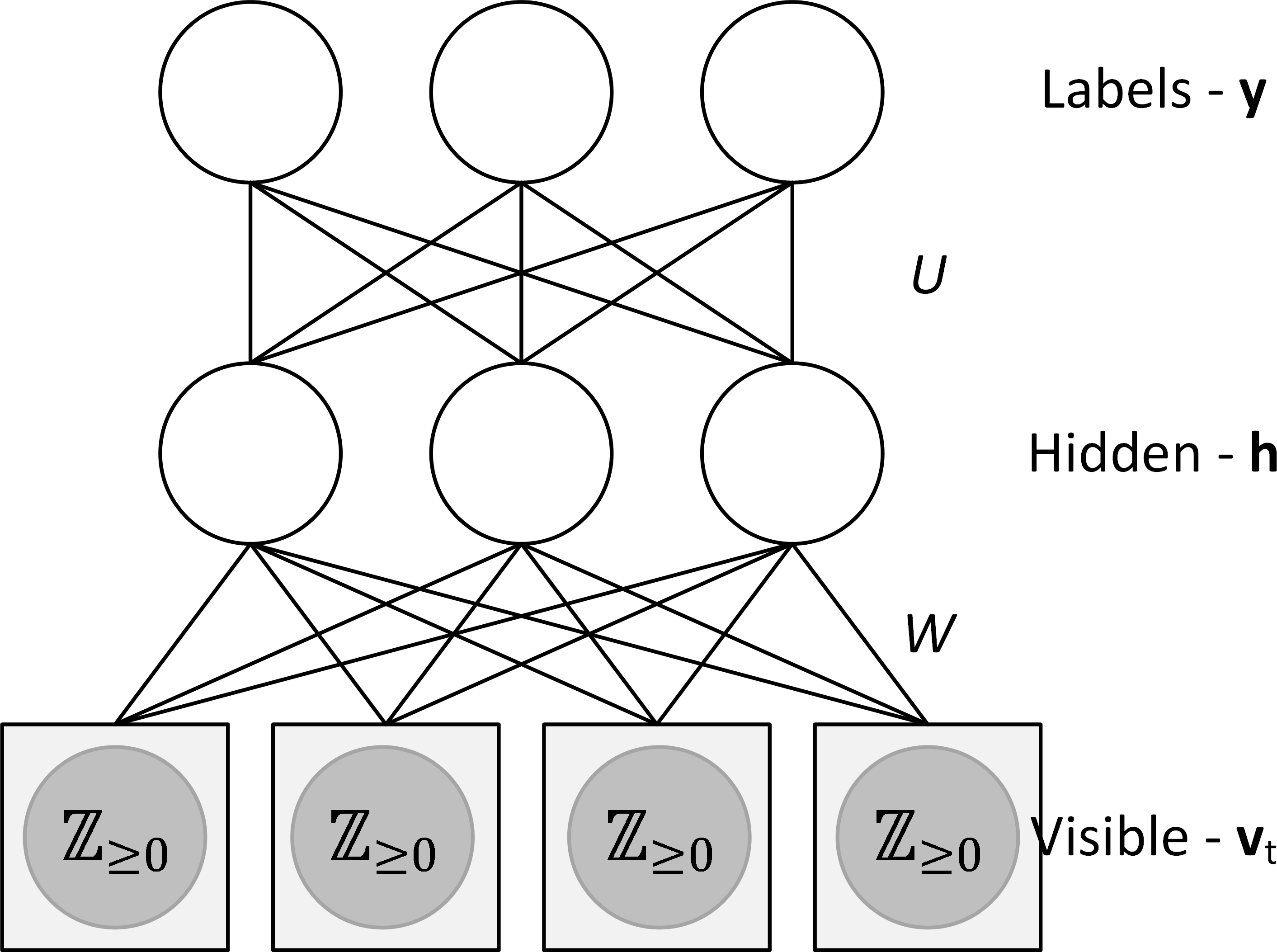
Figure 1: This figure illustrates the CountDCRBM model.

$$\centering\begin{array}[]{c}p_{\text{C}}({\bf v}_{t},{\bf h}_{t}|{\bf v}_{<t})=\exp[-E_{\text{C}}({\bf v}_{t},{\bf h}_{t}|{\bf v}_{<t})]/Z({\boldsymbol{\theta}}).\end{array}\@add@centering$$ (1)

The energy function $E_{\text{C}}({\bf v}_{t},{\bf h}_{t}|{\bf v}_{<t})$ in (2) is defined in a manner similar to that of the RBM.

The probability distributions for the visible nodes are defined in (3),

where, $\mathcal{N}$ is a normal distribution, $\sigma$ is a sigmoid distribution, and $\mathcal{P}$ is a Poisson distribution. The hidden nodes is defined in (4),

$$p_{\text{C}}(h_{j,t}=1|{\bf v}_{t},{\bf v}_{<t})=\sigma(d_{j}+\sum_{i}v_{i,t}w_{i,j}).$$ (4)

$$c_{i}=a_{i}+\sum_{p}A_{p,i}v_{p,<t},\quad d_{j}=b_{j}+\sum_{p}B_{p,j}v_{p,<t}.$$ (5)

Discriminative CRBMs: DCRBMs are based on the model in (Larochelle & Bengio, 2008), generalized to account for temporal phenomenon using CRBMs. DCRBMs are a simpler version of the Factored Conditional Restricted Boltzmann Machines (Taylor et al., 2011) and Gated Restricted Boltzmann Machines (Memisevic & Hinton, 2007). Both these models incorporate labels in learning representations, however, they use a more complicated potential which involves three way connections into factors. DCRBMs define the probability distribution $p_{\text{DC}}$ as a Gibbs distribution (6).

The hidden layer ${\bf h}$ is defined as a function of the labels $y$ and the visible nodes ${\bf v}$. A new probability distribution for the classifier is defined to relate the label $y$ to the hidden nodes ${\bf h}$ as in (7), as well as relate ${\bf h}$ to $y$ as in (8). The new energy function $E_{\text{DC}}$ is shown in (9).

$$p_{\text{DC}}(y_{l,t}|{\bf h}_{t})=\frac{\exp[s_{l}+\sum_{j}u_{j,l}h_{j,t}]}{\sum_{l^{*}}\exp[s_{l^{*}}+\sum_{j}u_{j,l^{*}}h_{j,t}]}$$ (8)

Count-DCRBMs: We extend the DCRBM to CountDCRBM Figure 1. Count-DCRBMs are based on the model in (Salakhutdinov & Hinton, 2009), generalized to account for temporal phenomenon using CRBMs, and discriminative classification. Count-DCRBMs are used to model time varying histograms of counts. The probability distribution over the visible layer will follow a constrained Poisson distribution, $p_{\text{C-Count}}(v_{i,t}|{\bf h}_{t},{\bf v}_{<t})$ defined in (3), the hidden layer follows (7) and the label layer follows (8) and the energy function $E_{\text{C-Count}}({\bf v}_{t},{\bf h}_{t}|{\bf v}_{<t})$ defined in (9).

4 Inference and Learning

Inference: to perform classification at time $t$ in the CountDCRBM given ${\bf v}_{<t}$ and ${\bf v}_{t}$ we use a bottom-up approach, computing a cost for each possible label ${\bf y}_{t}$ then choosing the label with least cost. We compute the cost for label ${\bf y}_{t}$ to be the free energy $-\log p_{\text{DC}}({\bf y}_{t},{\bf v}_{t}|{\bf v}_{<t})$ computed by marginalizing over ${\bf h}_{<t}$ and ${\bf h}_{t}$. Then, the cost associated with the candidate label is the free energy in the CountDCRBM, namely $-\log p_{\text{DC}}({\bf y}_{t},{\bf h}_{t}|{\bf h}_{<t})$ is tractable, because the sum over exponentially many terms can be algebraically eliminated.

Learning: the parameters our model could be learned using Contrastive Divergence (CD) (Hinton, 2002), where $\langle\cdot\rangle_{data}$ is the expectation with respect to the data distribution and $\langle\cdot\rangle_{recon}$ is the expectation with respect to the reconstructed data. The learning is done using two steps a bottom-up pass and a top-down pass using sampling equations from (3), (7), and (8). Bottom-up: the reconstruction is generated by first sampling the hidden layer $p(h_{t,j}=1|{\bf v}_{t},{\bf v}_{<t},y_{l})$ for all the hidden nodes in parallel. Top-down: This is followed by sampling the visible nodes $p(v_{i,t}|{\bf h}_{t},{\bf v}_{<t})$ and $p(y_{l,t}|{\bf h}_{t},{\bf h}_{<t})$ for all the visible nodes in parallel.

5 Experiments

We used the open-source simulator GPGPU-Sim (Bakhoda et al., 2009) to generate data to validate our approach. The simulator has been verified rigorously for accuracy against on a suite of 80 microbenchmarks (Leng et al., 2013). We used the BACKProp problem from the RODINIA benchmark (Che et al., 2010), and simulate a NVIDIA GTX480 GPU with the default configurations for GPGPU-Sim. This benchmark CUDA program trains a feedforward neural network with one hidden layer consisting of 4096 units.

To generate our dataset, we modified GPGPU-Sim to retrieve the time-indexed list of instruction mix, ie.​ for each time cycle the number of different instruction types based on opcode. These are the visible units in our model. We tested our approach on three different caches (Instruction (IC), Data Read (D_R), Data Write (D_W)) localized within one core of the GPU. For each cache, GPGPU-Sim outputs a list of time-indexed binary labels corresponding to whether a cache miss occured. Since we want to predict a cache miss ahead of time, we aggregated the labels over $128$ cycles so a label of $y(t)=1$ means that a cache miss occurred in cycles $[t,t+128]$.

The Count-DCRBM was trained on a Tesla K20C GPU using Contrastive Divergence with a constant learning rate of $10^{-5}$. Table 1 shows the final accuracies of a model with $15$ hidden nodes and varying temporal history available for DCRBM. The second and third columns are metrics that describe predictive power, taking into account false positives and negatives. We observe high accuracy and predictive power of the model for all three caches. We also observe that increased history generally leads to better performance despite the increased model complexity. Our baseline is an SVM that uses the raw instruction mix as features without any temporal history.

Model accuracy can be misleading because cache miss events are rare (e.g. about 10% for IC). Figure 3 (Top) shows these metrics over training epochs for data write cache. Note that the initial model accuracy is already about 70% where the model predicts that cache miss never occurs, with a corresponding metric F1 and Mathew Correlation Coefficient (MCC) value of zero. As training epochs increase, we note a sharp increase in predictive power around 5000 epochs. We also show the reconstruction error in Figure 3 (Middle), the objective value for training, over epochs for the data write cache. We observe that the reconstruction error significantly drops in the first 20k epochs. Figure 3 (Bottom) shows a measure of the classification error, measured in terms of the binary cross entropy between the true and predicted labels. We also observe that the classification error continues to drop steadily even though the reconstruction error has converged, showing that the model accounts for label information. Figure 3 shows the prediction using a history of 10 cycles, in comparison with the ground truth. Future work includes validating our approach across microbenchmarks.

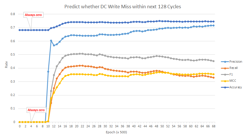
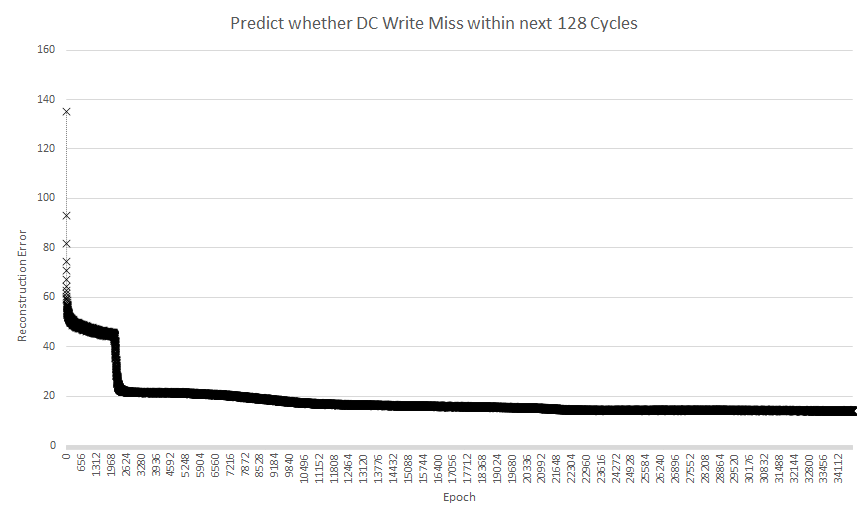
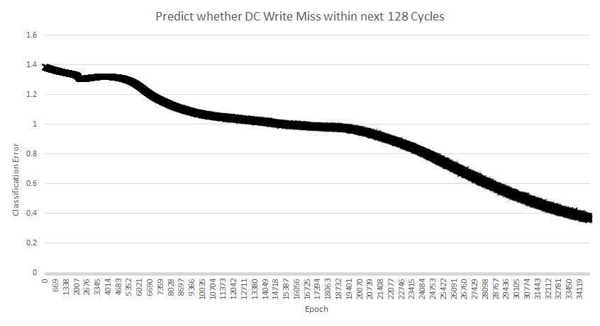
Figure 2: (Top) Accuracy (dark blue), precision light in light blue, recall in red, MCC in yellow, F1 in grey, (Middle) Reconstruction Error, (Bottom) Classification Error

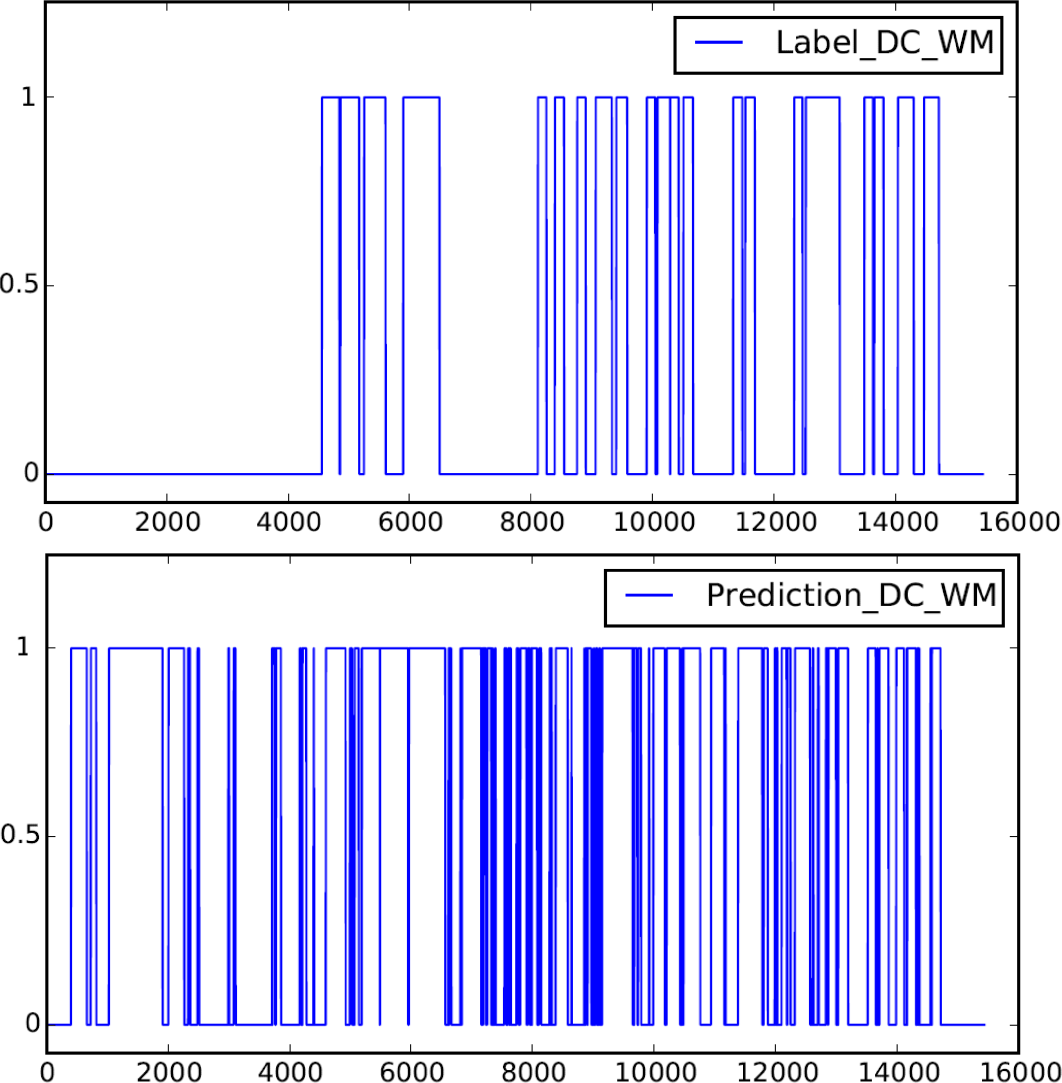
Figure 3: (Top) Ground truth labels, (Bottom) Prediction

Cache	Model	MCC	F1	Accuracy
DC_R	DCRBM(1)	0.32	0.59	0.67
	DCRBM(5)	0.35	0.63	0.68
	DCRBM(10)	0.39	0.66	0.69
	SVM(Poly)	0.34	0.44	0.83
	SVM(RBF)	0.41	0.51	0.83
DC_W	DCRBM(1)	0.36	0.58	0.70
	DCRBM(5)	0.36	0.59	0.65
	DCRBM(10)	0.32	0.58	0.65
	SVM(Poly)	0.27	0.31	0.64
	SVM(RBF)	0.32	0.55	0.68
IC	DCRBM(1)	0.32	0.40	0.86
	DCRBM(5)	0.32	0.39	0.87
	DCRBM(10)	0.37	0.44	0.85
	SVM(Poly)	0	0	0.99
	SVM(RBF)	0	0	0.98

Table 1: Scores vs Models for different types of cache. The larger the history for DCRBM, the higher the complexity and training difficulty of the model. Larger history is better except in the case of Data Write.

6 Conclusions

Our approach has significant implications for the GPU revolution of computing. A data driven approach can potentially identify mix of instructions that cause performance bottlenecks. Although we focused on cache misses, any statistic of interest to the computer architecture community such as power consumption and voltage can potentially be predicted. The extension to an online embedded setting is straightforward and could potentially save computation time. Prediction of performance bottlenecks is a step towards a cognitive processor architecture.

References

- Bakhoda et al. (2009) Bakhoda, Ali, Yuan, George L, Fung, Wilson WL, Wong, Henry, and Aamodt, Tor M. Analyzing Cuda Workloads Using a Detailed GPU Simulator. In IEEE International Symposium on Performance Analysis of Systems and Software (ISPASS), 2009.
- Ball & Larus. (1993) Ball, Thomas and Larus., James R. Branch Prediction for Free. In ACM, 1993.
- Bergman et al. (2008) Bergman, Keren et al. ExaScale Computing Study: Technology Challenges in Achieving Exascale Systems. volume 15, 2008.
- Blem et al. (2011) Blem, Emily, Sinclair, Matthew, and Sankaralingam, Karthikeyan. Challenge Benchmarks that must be Conquered to Sustain the GPU Revolution. CELL, 2011.
- Calder & et al. (1997) Calder, Brad and et al. Evidence-based Static Branch Prediction using Machine Learning. In ACM Transactions on Programming Languages and Systems (TOPLAS), 1997.
- Che et al. (2010) Che, Shuai, Sheaffer, Jeremy W, Boyer, Michael, Szafaryn, Lukasz G, Wang, Liang, and Skadron, Kevin. A Characterization of the Rodinia Benchmark Suite with Comparison to Contemporary CMP Workloads. In IISWC, 2010.
- Chen et al. (2014) Chen, Xuhao, Chang, Li-Wen, Rodrigues, Christopher I, Lv, Jie, Wang, Zhiying, and Hwu, Wen-Mei. Adaptive Cache Management for Energy-efficient GPU Computing. In Microarchitecture, 2014.
- Esmaeilzadeh & et. al. (2011) Esmaeilzadeh, Hadi and et. al. Dark Silicon and the End of Multicore Scaling. In Proceedings of the International Symposium on Computer Architecture (ISCA), 2011.
- Fung et al. (2007) Fung, Wilson WL, Sham, Ivan, Yuan, George, and Aamodt, Tor M. Dynamic Warp Formation and Scheduling for Efficient GPU Control Flow. In Proceedings of the 40th Annual IEEE/ACM International Symposium on Microarchitecture, 2007.
- Hinton (2002) Hinton, Geoffrey E. Training Products of Experts by Minimizing Contrastive Divergence. MIT Press, 2002.
- Hinton et al. (2006) Hinton, Geoffrey E, Osindero, Simon, and Teh, Yee-Whye. A Fast Learning Algorithm for Deep Belief Nets. MIT Press, 2006.
- Jiménez & Lin (2001) Jiménez, Daniel A and Lin, Calvin. Dynamic Branch Prediction with Perceptrons. In High-Performance Computer Architecture, 2001. HPCA. The Seventh International Symposium on. IEEE, 2001.
- Larochelle & Bengio (2008) Larochelle, H. and Bengio, Y. Classification using Discriminative Restricted Boltzmann Machines. In ICML, 2008.
- Lee et al. (2010) Lee, Jaekyu, Lakshminarayana, Nagesh B, Kim, Hyesoon, and Vuduc, Richard. Many-thread Aware Prefetching Mechanisms for GPGPU Applications. In Microarchitecture, 2010.
- Leng et al. (2013) Leng, Jingwen, Hetherington, Tayler, El Tantawy, Ahmed, Gilani, Syed, Kim, Nam Sung, Aamodt, Tor M, and Reddi, Vijay Janapa. GPUWattch:Enabling Energy Optimizations in GPGPUs. ACM SIGARCH, 2013.
- Leng et al. (2015) Leng, Jingwen, Buyuktosunoglu, Alper, Bertran, Ramon, Bose, Pradip, and Reddi, Vijay Janapa. Safe Limits on Voltage Reduction Efficiency in GPUs: A Direct Measurement Approach. In Microarchitecture. ACM, 2015.
- Li et al. (2015) Li, Dong, Rhu, Minsoo, Johnson, Daniel R, O’Connor, Mike, Erez, Mattan, Burger, Doug, Fussell, Donald S, and Redder, Stephen W. Priority-based Cache Allocation in Throughput Processors. In HPCA, 2015.
- Memisevic & Hinton (2007) Memisevic, R. and Hinton, G. E. Unsupervised Learning of Image Transformations. In CVPR, 2007.
- Mohamed & Hinton (2009) Mohamed, A. R. and Hinton, G. E. Phone Recognition using Restricted Boltzmann Machines. In ICASSP, 2009.
- Patterson (2006) Patterson, David. Future of Computer Architecture. In Berkeley EECS Annual Research Symposium, 2006.
- S. Chai (2014) S. Chai, et al. Lightweight Detection and Recovery Mechanisms to Extend Algorithm Resiliency in Noisy Computation. In WNTC, 2014.
- Salakhutdinov & Hinton (2006) Salakhutdinov, R. and Hinton, G. E. Reducing the Dimensionality of Data with Neural Networks. In Science, 2006.
- Salakhutdinov & Hinton (2009) Salakhutdinov, Ruslan and Hinton, Geoffrey. Semantic Hashing. In International Journal of Approximate Reasoning, 2009.
- Sutskever & Hinton (2007) Sutskever, I. and Hinton, G. E. Learning Multilevel Distributed Representations for High-Dimensional Sequences. In AISTATS, 2007.
- Taylor et al. (2011) Taylor, Graham W., Hinton, Geoffrey E., and Roweis, Sam T. Two Distributed-State Models For Generating High-Dimensional Time Series. In Journal of Machine Learning Research, 2011.
- Tiwari et al. (1994) Tiwari, Vivek, Malik, Sharad, and Wolfe, Andrew. Power Analysis of Embedded Software: A First Step Towards Software Power Minimization. VLSI Systems, 1994.
- Wulf & McKee (1995) Wulf, Wm A. and McKee, Sally A. Hitting the Memory Wall: Implications of the Obvious. In ACM SIGARCH computer architecture news, 1995.
- Yeh & Patt (1991) Yeh, Tse-Yu and Patt, Yale N. Two-level Adaptive Training Branch Prediction. In ACM ISM, 1991.