A pedestrian flow model with stochastic velocities: microscopic and macroscopic approaches

S. Göttlich111University of Mannheim, Department of Mathematics, 68131 Mannheim, Germany (goettlich@uni-mannheim.de, stknapp@mail.uni-mannheim.de).,   S. Knapp11footnotemark: 1,   P. Schillen11footnotemark: 1
Abstract

We investigate a stochastic model hierarchy for pedestrian flow. Starting from a microscopic social force model, where the pedestrians switch randomly between the two states stop-or-go, we derive an associated macroscopic model of conservation law type. Therefore we use a kinetic mean-field equation and introduce a new problem-oriented closure function. Numerical experiments are presented to compare the above models and to show their similarities.

AMS Classification. 90B20, 65Cxx, 35L60

Keywords. interacting particle system, stochastic processes, mean field equations, hydrodynamic limit, macroscopic pedestrian model, numerical simulations

1 Introduction

The modeling of crowd dynamics is a current research topic and provides a useful tool for evacuation planning. A good overview of the existing literature can be found in [4, 7], where mainly two classes of modeling approaches (microscopic versus macroscopic) are distinguished. Microscopic pedestrian models typically rely on Newton-type dynamics as proposed e.g. in [13, 20] while macroscopic models can be either derived via limiting processes [6, 7, 18] or phenomenologically, see e.g. [12, 14, 20, 21]. Starting from a microscopic level model extensions include for example vision cones [8], shortest-path information [10] and diffusion [7, 10].

In this work, we focus on a well-known phenomenon in crowds which is the sudden presence of non-moving people stopping immediately due to external attractions or, more recently, new cell phone messages. This leads to significant changes in the individual walking velocities, rerouting actions and hence to local bottlenecks depending on the crowd density. From reality we observe that people stop directly in front of attractions at a high probability and therefore influence other individuals also to stop or keep on walking. This random effect will be included as a stochastic process which is dependent on the position of the pedestrians. The main difference to existing pedestrian models with random effects is the motivation mentioned above and the mathematical representation of the stochastic dynamics. Similar problems have been considered in e.g. [7, 10, 18], where a formulation of the dynamical system in terms of Brownian motion driven stochastic differential equations (SDEs) has been used to capture intrinsic random decisions in the velocity of pedestrians. However, this approach is not suitable to cover the stop-and-go behavior of pedestrians we have in mind. We will use a continuous-time Markov chain approach [9] to include the random stop-and-go behavior by considering location-dependent switching rates. The overall goal is then to derive a model hierarchy for the microscopic and macroscopic pedestrian flow. In a first step, we develop and define the stochastic microscopic pedestrian model based on the social force model by Helbing and Molnár [13] and prove its existence, see section 2. Then, the kinetic formulation of the microscopic model under the molecular chaos assumption in terms of measures is considered. The derivation of a reasonable closure function to state the associated macroscopic pedestrian model is non-standard and requires some computational effort. Section 3 deals with the numerical treatment of the microscopic and macroscopic equations. We present a stochastic simulation algorithm for the microscopic model and explain how numerical methods for hyperbolic conservation laws can be used to approximate the solution of the macroscopic model. For simulation purposes we present two examples in section 4 and compare qualitatively both approaches by defining reasonable performance measures. An additional experiment with a deterministic situation, i.e., no random velocity drops to zero, will be also discussed.

The following picture 1 summarizes the main properties of the deterministic and stochastic modeling approach for different levels of descriptions. It intends to give an idea on the main ingredients used throughout the sections 2 to 4.

Scalar conservation law with advection part only One velocity model: Pedestrians always move with the closure velocity System of conservation laws with advection and reaction part Two velocities model: Pedestrians may change their velocities (stop or go) Variables: position and velocities Time-continuous Newton-type dynamics Variables: position, velocities and status (stop or go) Time-discrete stochastic process Deterministic Stochastic Microscopic Macroscopic
Figure 1: Overview of the deterministic and stochastic model hierarchy

2 The Models

In this section, we derive a stochastic microscopic model and deduce a corresponding macroscopic model. First, we define the stochastic microscopic model based on a deterministic social force model [13] and show its well-posedness. Second, we determine the time-evolution of the microscopic model and use a mean field assumption to get a kinetic model. This model is then simplified by an appropriate closure assumption to develop a macroscopic model, cf. existing literature on particle systems, e.g. [5, 16, 17, 18] and pedestrian flow models in e.g. [7].

2.1 Microscopic Model

We use the ideas introduced by Helbing and Molnár [13] to describe the dynamical behavior of pedestrians. Let N𝑁absentN\in\N be the number of pedestrians and let

xi(t)=(xi(1)(t),xi(2)(t))2x_{i}(t)=(x_{i}^{(1)}(t),x_{i}^{(2)}(t))\in{}^{2}

the position of pedestrian i𝑖i at time t0t\in{}_{\geq 0}. The velocity of pedestrian i𝑖i at time t𝑡t is given by

x˙i(t)=vi(t)=(vi(1)(t),vi(2)(t)).2\dot{x}_{i}(t)=v_{i}(t)=(v_{i}^{(1)}(t),v_{i}^{(2)}(t))\in{}^{2}.

In the following, we denote by

x(t)=(x1(t),,xN(t))2N\vec{x}(t)=(x_{1}(t),\dots,x_{N}(t))\in{}^{2N}

and

v(t)=(v1(t),,vN(t))2N\vec{v}(t)=(v_{1}(t),\dots,v_{N}(t))\in{}^{2N}

the states of the system consisting of N𝑁N pedestrians. The model equations are of Newton-type dynamics

x˙i(t)subscript˙𝑥𝑖𝑡\displaystyle\dot{x}_{i}(t) =V(xi(t),vi(t)),absent𝑉subscript𝑥𝑖𝑡subscript𝑣𝑖𝑡\displaystyle=V(x_{i}(t),v_{i}(t)),
v˙i(t)subscript˙𝑣𝑖𝑡\displaystyle\dot{v}_{i}(t) =Fdest(xi(t),vi(t))+Fiint(x(t),v(t))absentsuperscript𝐹𝑑𝑒𝑠𝑡subscript𝑥𝑖𝑡subscript𝑣𝑖𝑡superscriptsubscript𝐹𝑖𝑖𝑛𝑡𝑥𝑡𝑣𝑡\displaystyle=F^{dest}(x_{i}(t),v_{i}(t))+F_{i}^{int}(\vec{x}(t),\vec{v}(t)) (2.1)

with initial positions x(0)=x02N\vec{x}(0)=\vec{x}_{0}\in{}^{2N} and velocities v(0)=v02N\vec{v}(0)=\vec{v}_{0}\in{}^{2N}. The acting forces are divided into the destination force Fdestsuperscript𝐹𝑑𝑒𝑠𝑡F^{dest} and the interaction force Fiintsuperscriptsubscript𝐹𝑖𝑖𝑛𝑡F_{i}^{int}. The determination of boundary and obstacles forces is done using the function V𝑉V adapted from swarming models [1, 2]. We remark that the equations (2.1) are non-standard in the sense that the first equation on x˙i(t)subscript˙𝑥𝑖𝑡\dot{x}_{i}(t) is not dependent on the velocity vi(t)subscript𝑣𝑖𝑡v_{i}(t) only. The motivation of V(xi(t),vi(t))𝑉subscript𝑥𝑖𝑡subscript𝑣𝑖𝑡V(x_{i}(t),v_{i}(t)) will be explained more detailed in the paragraph on obstacle forces.

To keep the notation and calculations well-arranged, we keep the basic model simple and focus on the new modeling ideas.

Interaction and Destination Forces

As in [13], the interaction force acting on pedestrian i𝑖i is

Fiint(x(t),v(t)):=1N1j=1jiNG(xi(t)xj(t)),assignsuperscriptsubscript𝐹𝑖𝑖𝑛𝑡𝑥𝑡𝑣𝑡1𝑁1superscriptsubscript𝑗1𝑗𝑖𝑁𝐺subscript𝑥𝑖𝑡subscript𝑥𝑗𝑡F_{i}^{int}(\vec{x}(t),\vec{v}(t)):=\frac{1}{N-1}\sum_{\begin{subarray}{c}j=1\\ j\neq i\end{subarray}}^{N}G(x_{i}(t)-x_{j}(t)),

where G:2G\colon\R\to{}^{2} is a given vector field describing the repulsion and attraction.
Let vC>0superscript𝑣𝐶0v^{C}>0 be the comfort speed which is achieved approximately in the relaxation time τ>0𝜏0\tau>0. We define the destination force by

Fdest(xi(t),vi(t)):=1τ(vCD(xi(t))vi(t)),assignsuperscript𝐹𝑑𝑒𝑠𝑡subscript𝑥𝑖𝑡subscript𝑣𝑖𝑡1𝜏superscript𝑣𝐶𝐷subscript𝑥𝑖𝑡subscript𝑣𝑖𝑡F^{dest}(x_{i}(t),v_{i}(t)):=\frac{1}{\tau}\left(v^{C}D(x_{i}(t))-v_{i}(t)\right),

where D:22D\colon{}^{2}\to{}^{2} describes the direction to the destination of a pedestrian at position xi(t)subscript𝑥𝑖𝑡x_{i}(t). If xD2x^{D}\in{}^{2} is some destination point, then D𝐷D can be expressed in the simplest case by

D(x)=xDxxDx.𝐷𝑥superscript𝑥𝐷𝑥normsuperscript𝑥𝐷𝑥D(x)=\frac{x^{D}-x}{||x^{D}-x||}.

Note that alternative destination directions could be achieved by considering the shortest path between the current position x𝑥x and the destination xDsuperscript𝑥𝐷x^{D} by solving the Eikonal equation, see e.g. [10].

Obstacle Forces

Different to [13], we choose an alternative way to model the obstacle forces by applying a kind of specular reflection, see [1, 2]. The reason for this choice is that singular forces can occur close to obstacles leading to numerical difficulties during the simulation of (2.1).

Let Γ2\Gamma\subset{}^{2} be a domain with outer normal unit field n𝑛\vec{n} which is continuous and defined on Γ¯¯Γ\overline{\Gamma}. The boundary ΓΓ\partial\Gamma describes walls as well as obstacles and the outer normal field allows to manipulate the velocity vector such that pedestrians walk along these boundaries. We assume a pedestrian very close to a wall at position xΓ𝑥Γx\in\Gamma having a velocity vector v2v\in{}^{2} which is given by the destination and interaction forces. The position at a later time is then given by x+Δtv𝑥Δ𝑡𝑣x+\Delta tv and might be outside of the domain, see figure 2.

0.50.5-0.50.50.50.51111.51.51.50.50.5-0.50.50.50.51111.51.51.5v𝑣vx𝑥x
(a)
0.50.5-0.50.50.50.51111.51.51.50.50.5-0.50.50.50.51111.51.51.5vsuperscript𝑣v^{\ast}x𝑥xv𝑣vv~~𝑣\tilde{v}
(b)
Figure 2: Velocity vector at the boundary

This is the case if the vector v𝑣v points out of the domain, i.e., vn0𝑣𝑛0v\cdot\vec{n}\geq 0. In the other case vn<0𝑣𝑛0v\cdot\vec{n}<0, the pedestrian walks into the domain and the velocity vector is admissible. Let d(x,Γ)𝑑𝑥Γd(x,\partial\Gamma) be the distance to the boundary and Uϵ={x:2d(x,Γ)ϵ}U_{\epsilon}=\{x\in{}^{2}\colon d(x,\partial\Gamma)\leq\epsilon\} the zone, where pedestrians feel uncomfortable close to a wall or obstacle. We avoid the collision with the boundary by an orthogonal projection of the point x+Δtv𝑥Δ𝑡𝑣x+\Delta tv onto the tangent space at x𝑥x spanned by the orthogonal vector

n(x)=(n2(x),n1(x))Tsuperscript𝑛perpendicular-to𝑥superscriptsubscript𝑛2𝑥subscript𝑛1𝑥𝑇\vec{n}^{\perp}(x)=(-n_{2}(x),n_{1}(x))^{T}

to the outer unit normal vector. For the projected point, it follows

Π(x+Δtv)=x+Δtvn(x)n(x)Π𝑥Δ𝑡𝑣𝑥Δ𝑡𝑣superscript𝑛perpendicular-to𝑥superscript𝑛perpendicular-to𝑥\Pi(x+\Delta tv)=x+\Delta tv\cdot\vec{n}^{\perp}(x)\vec{n}^{\perp}(x)

and to conserve the velocity by the projection, we set

v~(v,x)=vvn(x)|vn(x)|n(x)=vsgn(vn(x))n(x)~𝑣𝑣𝑥norm𝑣𝑣superscript𝑛perpendicular-to𝑥𝑣superscript𝑛perpendicular-to𝑥superscript𝑛perpendicular-to𝑥norm𝑣sgn𝑣superscript𝑛perpendicular-to𝑥superscript𝑛perpendicular-to𝑥\tilde{v}(v,x)=||v||\frac{v\cdot\vec{n}^{\perp}(x)}{|v\cdot\vec{n}^{\perp}(x)|}\vec{n}^{\perp}(x)=||v||\operatorname{sgn}{(v\cdot\vec{n}^{\perp}(x))}\vec{n}^{\perp}(x)

such that v~(v,x)=vnorm~𝑣𝑣𝑥norm𝑣||\tilde{v}(v,x)||=||v|| holds. Due to the assumption that a pedestrian will not change the direction immediately at the obstacle, we take a sufficiently smooth increasing function J:[0,)[0,1]:𝐽001J\colon[0,\infty)\to[0,1] with J(0)=0𝐽00J(0)=0 and J(1)=1𝐽11J(1)=1 and define

v(v,x)=v~(v,x)+J(d(x,Γ)ϵ)(vv~(v,x))superscript𝑣𝑣𝑥~𝑣𝑣𝑥𝐽𝑑𝑥Γitalic-ϵ𝑣~𝑣𝑣𝑥v^{\ast}(v,x)=\tilde{v}(v,x)+J\left(\frac{d(x,\partial\Gamma)}{\epsilon}\right)(v-\tilde{v}(v,x))

Summarizing, the velocity vector is given by

V(x,v):={v if vn(x)<0 and v(v,x)vv(v,x) if vn(x)0assign𝑉𝑥𝑣cases𝑣 if 𝑣𝑛𝑥0 and superscript𝑣𝑣𝑥norm𝑣normsuperscript𝑣𝑣𝑥 if 𝑣𝑛𝑥0V(x,v):=\begin{cases}v&\text{ if }v\cdot\vec{n}(x)<0\text{ and }\\ v^{\ast}(v,x)\frac{||v||}{||v^{\ast}(v,x)||}&\text{ if }v\cdot\vec{n}(x)\geq 0\end{cases}

and one can easily check that V(x,v)=vnorm𝑉𝑥𝑣norm𝑣||V(x,v)||=||v||.

Random Velocity Effects

All forces (interaction, destination and obstacle) considered so far are purely deterministic and include no random effects. Different to pedestrian models modeled by SDEs, we choose an alternative way to include random effects. From phenomenological observations we deduce the intrinsic random effect that pedestrians can decide to walk or to stop independently of each other. This can be done by switching the velocity and acceleration to zero and back again. More precisely, an individual that stops immediately will keep on walking again after a random time.

To include this phenomenon mathematically we describe the positions, velocities and the status, i.e.,  stop or go, as a time discrete stochastic process. Let Δt>0Δ𝑡0\Delta t>0 be a small fixed time stepsize and let xin2x_{i}^{n}\in{}^{2} the position, vin2v_{i}^{n}\in{}^{2} the velocity and rin{0,1}superscriptsubscript𝑟𝑖𝑛01r_{i}^{n}\in\{0,1\} the status of pedestrian i𝑖i at time tn=nΔtsubscript𝑡𝑛𝑛Δ𝑡t_{n}=n\Delta t for n0n\in{}_{0}.

To ease the notation, we denote by Fi=Fdest+Fiintsubscript𝐹𝑖superscript𝐹𝑑𝑒𝑠𝑡superscriptsubscript𝐹𝑖𝑖𝑛𝑡F_{i}=F^{dest}+F_{i}^{int} the sum of forces acting on pedestrian i𝑖i.

We consider a stochastic process X=(Xn,n)0X=(X^{n},n\in{}_{0}) with Xn=(xn,vn,rn)E(N)=×2N×2N{0,1}NX^{n}=(\vec{x}^{n},\vec{v}^{n},\vec{r}^{n})\in E^{(N)}={}^{2N}\times{}^{2N}\times\{0,1\}^{N} on some probability space (Ω,𝒜,P)Ω𝒜𝑃(\Omega,\mathcal{A},P) such that

P(xin+1\displaystyle P(x_{i}^{n+1} =xin+rinΔtV(xin,vin)|Xn)=1,\displaystyle=x_{i}^{n}+r_{i}^{n}\Delta tV(x_{i}^{n},v_{i}^{n})|X^{n})=1, (2.2)
P(vin+1\displaystyle P(v_{i}^{n+1} =vin+ΔtFi(xn,vn)|Xn)=rin,\displaystyle=v_{i}^{n}+\Delta tF_{i}(\vec{x}^{n},\vec{v}^{n})|X^{n})=r_{i}^{n}, (2.3)
P(vin+1\displaystyle P(v_{i}^{n+1} =0|Xn)=1rin, and\displaystyle=0|X^{n})=1-r_{i}^{n},\text{ and } (2.4)
P(rin+1\displaystyle P(r_{i}^{n+1} =z|Xn)=𝟙z(rin)(1Δtλ(rin,xin))+𝟙1z(rin)Δtλ(rin,xin)\displaystyle=z|X^{n})=\mathds{1}_{z}(r_{i}^{n})(1-\Delta t\lambda(r_{i}^{n},x_{i}^{n}))+\mathds{1}_{1-z}(r_{i}^{n})\Delta t\lambda(r_{i}^{n},x_{i}^{n}) (2.5)

for all i=1,,N𝑖1𝑁i=1,\dots,N, n0n\in{}_{0}, z{0,1}𝑧01z\in\{0,1\} and some rate function λ:{0,1}×20\lambda\colon\{0,1\}\times{}^{2}\to{}_{\geq 0}. The rate function λ𝜆\lambda describes the expected events per unit time and is a given parameter. To avoid doubling effects by the interaction forces and the effects arising from the rate function λ𝜆\lambda, the rate function is assumed to be only dependent on the position of the pedestrian i𝑖i itself. Equations (2.2)–(2.4) can be seen as an Euler approximation of the deterministic system (2.1) while equation (2.5) describes the probability to walk (z=1𝑧1z=1) or to stop (z=0𝑧0z=0) during the next time step tn+1subscript𝑡𝑛1t_{n+1} given the values of the process at time tnsubscript𝑡𝑛t_{n}. This idea is adapted from [9], where a continuous-time Markov Chains is used to motivate a production model with random breakdowns.

Note that for the approach (2.2)–(2.5), we can only expect a well-defined model if Δtλ(r,x)[0,1]Δ𝑡𝜆𝑟𝑥01\Delta t\lambda(r,x)\in[0,1]. Therefore we assume λ𝜆\lambda to be uniformly bounded and Δtλ1Δ𝑡superscriptsubscriptnorm𝜆1\Delta t\leq||\lambda||_{\infty}^{-1}. Furthermore, we have to fix an initial probability measure μ(N)0subscriptsuperscript𝜇0𝑁\mu^{0}_{(N)} on the measurable space (E(N),(N))superscript𝐸𝑁superscript𝑁(E^{(N)},\mathcal{E}^{(N)}), where we denote by (N)=σ(E(N))superscript𝑁𝜎superscript𝐸𝑁\mathcal{E}^{(N)}=\sigma(E^{(N)}) the smallest σ𝜎\sigma-algebra containing E(N)superscript𝐸𝑁E^{(N)}. Summarizing, we state the following definition.

Definition 2.1.

A time discrete stochastic process X𝑋X on some probability space (Ω,𝒜,Pμ(N)0)Ω𝒜superscript𝑃superscriptsubscript𝜇𝑁0(\Omega,\mathcal{A},P^{\mu_{(N)}^{0}}) with values in E(N)=×2N×2N{0,1}NE^{(N)}={}^{2N}\times{}^{2N}\times\{0,1\}^{N} and initial measure μ(N)0superscriptsubscript𝜇𝑁0\mu_{(N)}^{0} satisfying equations (2.2)–(2.5) is called a stochastic microscopic pedestrian model.

Now, we will show the well-posedness of the model. We define the mapping U:E(N)×(N)0U\colon E^{(N)}\times\mathcal{E}^{(N)}\to{}_{\geq 0} by

U((x,v,r),B):=z{0,1}N[ϵh(x,v,r,z)(B)i=1N(𝟙zi(ri)(1Δtλ(ri,xi))+𝟙1zi(ri)Δtλ(ri,xi))]assign𝑈𝑥𝑣𝑟𝐵subscript𝑧superscript01𝑁delimited-[]subscriptitalic-ϵ𝑥𝑣𝑟𝑧𝐵superscriptsubscriptproduct𝑖1𝑁subscript1subscript𝑧𝑖subscript𝑟𝑖1Δ𝑡𝜆subscript𝑟𝑖subscript𝑥𝑖subscript11subscript𝑧𝑖subscript𝑟𝑖Δ𝑡𝜆subscript𝑟𝑖subscript𝑥𝑖\displaystyle U((\vec{x},\vec{v},\vec{r}),B):=\sum_{\vec{z}\in\{0,1\}^{N}}\left[\epsilon_{h(\vec{x},\vec{v},\vec{r},\vec{z})}(B)\prod_{i=1}^{N}\left(\mathds{1}_{z_{i}}(r_{i})(1-\Delta t\lambda(r_{i},x_{i}))+\mathds{1}_{1-z_{i}}(r_{i})\Delta t\lambda(r_{i},x_{i})\right)\right] (2.6)

with vector valued function

h(x,v,r,z)=(x1+Δtr1V(x1,v1)xN+ΔtrNV(xN,vN)r1(v1+ΔtF1(x,v))rN(vN+ΔtFN(x,v))z).𝑥𝑣𝑟𝑧matrixmissing-subexpressionsubscript𝑥1Δ𝑡subscript𝑟1𝑉subscript𝑥1subscript𝑣1missing-subexpressionmissing-subexpressionsubscript𝑥𝑁Δ𝑡subscript𝑟𝑁𝑉subscript𝑥𝑁subscript𝑣𝑁missing-subexpressionsubscript𝑟1subscript𝑣1Δ𝑡subscript𝐹1𝑥𝑣missing-subexpressionmissing-subexpressionsubscript𝑟𝑁subscript𝑣𝑁Δ𝑡subscript𝐹𝑁𝑥𝑣missing-subexpression𝑧h(\vec{x},\vec{v},\vec{r},\vec{z})=\begin{pmatrix}&x_{1}+\Delta tr_{1}V(x_{1},v_{1})\\ &\vdots\\ &x_{N}+\Delta tr_{N}V(x_{N},v_{N})\\ &r_{1}(v_{1}+\Delta tF_{1}(\vec{x},\vec{v}))\\ &\vdots\\ &r_{N}(v_{N}+\Delta tF_{N}(\vec{x},\vec{v}))\\ &\vec{z}\end{pmatrix}.

Then, well-posedness can be obtained using the Markovian kernel property.

Theorem 2.2.

Let λ,V,Fdest,Fiint,i=1,,Nformulae-sequence𝜆𝑉superscript𝐹𝑑𝑒𝑠𝑡superscriptsubscript𝐹𝑖𝑖𝑛𝑡𝑖1𝑁\lambda,V,F^{dest},F_{i}^{int},i=1,\dots,N be measurable mappings, λ𝜆\lambda uniformly bounded and Δtλ1Δ𝑡superscriptsubscriptnorm𝜆1\Delta t\leq||\lambda||_{\infty}^{-1}. Then, the mapping U𝑈U defined by (2.6) is a Markovian kernel on (E(N),(N))superscript𝐸𝑁superscript𝑁(E^{(N)},\mathcal{E}^{(N)}).

Proof.

For simplicity, we identify x𝑥x as (x,v,r)𝑥𝑣𝑟(\vec{x},\vec{v},\vec{r}) in the following. The first step of the proof is to show that for every set B(N)𝐵superscript𝑁B\in\mathcal{E}^{(N)} the mapping xU(x,B)maps-to𝑥𝑈𝑥𝐵x\mapsto U(x,B) is measurable. In a second step, we have to prove that for every xE(N)𝑥superscript𝐸𝑁x\in E^{(N)} the mapping BU(x,B)maps-to𝐵𝑈𝑥𝐵B\mapsto U(x,B) is a probability measure on (E(N),(N))superscript𝐸𝑁superscript𝑁(E^{(N)},\mathcal{E}^{(N)}). From the assumptions we get that hh is a measurable mapping and hence xϵh(x)(B)maps-to𝑥subscriptitalic-ϵ𝑥𝐵x\mapsto\epsilon_{h(x)}(B) is measurable. The function λ𝜆\lambda is also measurable and the sum as well as the product of (2.6) are finite such that U(x,B)𝑈𝑥𝐵U(x,B) is measurable in x𝑥x.

The mapping U𝑈U consists of a finite sum of weighted Dirac measures on (E(N),(N))superscript𝐸𝑁superscript𝑁(E^{(N)},\mathcal{E}^{(N)}) and the assumption 0<Δtλ10Δ𝑡superscriptsubscriptnorm𝜆10<\Delta t\leq||\lambda||_{\infty}^{-1} implies that weights must be non-negative. So U𝑈U is a measure on (E(N),(N))superscript𝐸𝑁superscript𝑁(E^{(N)},\mathcal{E}^{(N)}) and it remains to show that U(x,E(N))=1𝑈𝑥superscript𝐸𝑁1U(x,E^{(N)})=1 to complete the proof. We calculate

U(x,E(N))𝑈𝑥superscript𝐸𝑁\displaystyle U(x,E^{(N)}) =z{0,1}N[i=1N(𝟙zi(ri)(1Δtλ(ri,xi))+𝟙1zi(ri)Δtλ(ri,xi))]absentsubscript𝑧superscript01𝑁delimited-[]superscriptsubscriptproduct𝑖1𝑁subscript1subscript𝑧𝑖subscript𝑟𝑖1Δ𝑡𝜆subscript𝑟𝑖subscript𝑥𝑖subscript11subscript𝑧𝑖subscript𝑟𝑖Δ𝑡𝜆subscript𝑟𝑖subscript𝑥𝑖\displaystyle=\sum_{z\in\{0,1\}^{N}}\left[\prod_{i=1}^{N}\left(\mathds{1}_{z_{i}}(r_{i})(1-\Delta t\lambda(r_{i},x_{i}))+\mathds{1}_{1-z_{i}}(r_{i})\Delta t\lambda(r_{i},x_{i})\right)\right]
=z1=01zN1=01i=1N1(𝟙zi(ri)(1Δtλ(ri,xi))+𝟙1zi(ri)Δtλ(ri,xi))absentsuperscriptsubscriptsubscript𝑧101superscriptsubscriptsubscript𝑧𝑁101superscriptsubscriptproduct𝑖1𝑁1subscript1subscript𝑧𝑖subscript𝑟𝑖1Δ𝑡𝜆subscript𝑟𝑖subscript𝑥𝑖subscript11subscript𝑧𝑖subscript𝑟𝑖Δ𝑡𝜆subscript𝑟𝑖subscript𝑥𝑖\displaystyle=\sum_{z_{1}=0}^{1}\dots\sum_{z_{N-1}=0}^{1}\prod_{i=1}^{N-1}\left(\mathds{1}_{z_{i}}(r_{i})(1-\Delta t\lambda(r_{i},x_{i}))+\mathds{1}_{1-z_{i}}(r_{i})\Delta t\lambda(r_{i},x_{i})\right)
zN=01(𝟙zN(rN)(1Δtλ(rN,xN))+𝟙1zN(rN)Δtλ(rN,xN))\displaystyle\;\cdot\sum_{z_{N}=0}^{1}\left(\mathds{1}_{z_{N}}(r_{N})(1-\Delta t\lambda(r_{N},x_{N}))+\mathds{1}_{1-z_{N}}(r_{N})\Delta t\lambda(r_{N},x_{N})\right)
=z1=01zN1=01i=1N1(𝟙zi(ri)(1Δtλ(ri,xi))+𝟙1zi(ri)Δtλ(ri,xi))1absentsuperscriptsubscriptsubscript𝑧101superscriptsubscriptsubscript𝑧𝑁101superscriptsubscriptproduct𝑖1𝑁1subscript1subscript𝑧𝑖subscript𝑟𝑖1Δ𝑡𝜆subscript𝑟𝑖subscript𝑥𝑖subscript11subscript𝑧𝑖subscript𝑟𝑖Δ𝑡𝜆subscript𝑟𝑖subscript𝑥𝑖1\displaystyle=\sum_{z_{1}=0}^{1}\dots\sum_{z_{N-1}=0}^{1}\prod_{i=1}^{N-1}\left(\mathds{1}_{z_{i}}(r_{i})(1-\Delta t\lambda(r_{i},x_{i}))+\mathds{1}_{1-z_{i}}(r_{i})\Delta t\lambda(r_{i},x_{i})\right)\cdot 1
=absent\displaystyle=\dots
=1absent1\displaystyle=1

and conclude that U𝑈U is a probability measure in the second component. ∎

The mapping U𝑈U describes the one step transition probability of the system and allows to define a Markovian semigroup of kernels. We choose the typical composition of Markovian kernels, see e.g. [3],

UU(x,B)𝑈𝑈𝑥𝐵\displaystyle U\circ U(x,B) :=EU(x,dy)U(y,B)assignabsentsubscript𝐸𝑈𝑥𝑑𝑦𝑈𝑦𝐵\displaystyle:=\int_{E}U(x,dy)U(y,B) (2.7)

and define

U0superscript𝑈0\displaystyle U^{0} :=IdassignabsentId\displaystyle:=\operatorname{Id} (2.8)
Unsuperscript𝑈𝑛\displaystyle U^{n} :=k=1𝑛U for n.assignabsent𝑘1𝑛𝑈 for 𝑛absent\displaystyle:=\underset{k=1}{\overset{n}{\circ}}\;U\text{ for }n\in\N. (2.9)

The family (Un,n)0(U^{n},n\in{}_{0}) is then a normal semigroup of Markovian kernels and we get the following well-posedness result.

Theorem 2.3.

Let λ,V,Fdest,Fiint,i=1,,Nformulae-sequence𝜆𝑉superscript𝐹𝑑𝑒𝑠𝑡superscriptsubscript𝐹𝑖𝑖𝑛𝑡𝑖1𝑁\lambda,V,F^{dest},F_{i}^{int},i=1,\dots,N be measurable mappings, λ𝜆\lambda uniformly bounded, Δtλ1Δ𝑡superscriptsubscriptnorm𝜆1\Delta t\leq||\lambda||_{\infty}^{-1} and μ(N)0subscriptsuperscript𝜇0𝑁\mu^{0}_{(N)} a probability measure on (E(N),(N))superscript𝐸𝑁superscript𝑁(E^{(N)},\mathcal{E}^{(N)}). Then, there exists a stochastic microscopic pedestrian model. Furthermore, the distribution of N𝑁N pedestrians at time step tnsubscript𝑡𝑛t_{n} is given by

μ(N)n(B)=E(N)Un(x,B)μ(N)0(dx)subscriptsuperscript𝜇𝑛𝑁𝐵subscriptsuperscript𝐸𝑁superscript𝑈𝑛𝑥𝐵subscriptsuperscript𝜇0𝑁𝑑𝑥\displaystyle\mu^{n}_{(N)}(B)=\int_{E^{(N)}}U^{n}(x,B)\mu^{0}_{(N)}(dx) (2.10)

for every B(N)𝐵superscript𝑁B\in\mathcal{E}^{(N)}.

Proof.

The state space E(N)superscript𝐸𝑁E^{(N)} is a polish space and we hence can use the Daniell-Kolmogorov theorem [3] which guarantees the existence of a canonical coordinate process X=(Xn,n)0X=(X^{n},n\in{}_{0}) on some probability space (Ω,𝒜,Pμ(N)0)Ω𝒜superscript𝑃subscriptsuperscript𝜇0𝑁(\Omega,\mathcal{A},P^{\mu^{0}_{(N)}}) defined by the semigroup of Markovian kernels (Un,n)0(U^{n},n\in{}_{0}), cf. (2.9). The stochastic process X𝑋X is a Markov process and therefore (2.10) and

Pμ(N)0(Xn+1B|Xn=x)=U(x,B)superscript𝑃subscriptsuperscript𝜇0𝑁superscript𝑋𝑛1conditional𝐵superscript𝑋𝑛𝑥𝑈𝑥𝐵P^{\mu^{0}_{(N)}}(X^{n+1}\in B|X^{n}=x)=U(x,B)

are satisfied. By setting x=(x,v,r)𝑥𝑥𝑣𝑟x=(\vec{x},\vec{v},\vec{r}) and

B={x1+r1ΔtV(x1,v1)}××2(N1)×2N{0,1}NB=\{x_{1}+r_{1}\Delta tV(x_{1},v_{1})\}\times{}^{2(N-1)}\times{}^{2N}\times\{0,1\}^{N}

we obtain equation (2.2) in the case i=1𝑖1i=1. The remaining equations (2.3)–(2.5) can be deduced analogously. ∎

2.2 Kinetic Model

We now analyze the evolution of measures given by the microscopic pedestrian flow model. The principal idea is to derive the Kolmogorov forward equation, see e.g. [11], given by the semigroup (Un,n)0(U_{n},n\in{}_{0}). To do so, we introduce the following spaces of test-functions 𝒞(N)superscript𝒞𝑁\mathcal{C}^{(N)} and 𝒞𝒞\mathcal{C} to capture the discrete states of the pedestrians:

𝒞(N)superscript𝒞𝑁\displaystyle\mathcal{C}^{(N)} :=assign\displaystyle:= {ϕ:E(N):ϕ(x,v,) is 𝒫({0,1}N)/()-measurable,ϕ(,,r)Cb1(×2N;2N)}\displaystyle\{\phi\colon E^{(N)}\to\R\colon\phi(\vec{x},\vec{v},\cdot)\text{ is }\mathcal{P}(\{0,1\}^{N})/\mathcal{B}(\R)\text{-measurable},\phi(\cdot,\cdot,\vec{r})\in C_{b}^{1}({}^{2N}\times{}^{2N};\R)\}
𝒞𝒞\displaystyle\mathcal{C} :=assign\displaystyle:= {ψ:E:ψ(x,v,) is 𝒫({0,1})/()-measurable,ψ(,,r)Cb1(×2;2)},\displaystyle\{\psi\colon E\to\R\colon\psi(x,v,\cdot)\text{ is }\mathcal{P}(\{0,1\})/\mathcal{B}(\R)\text{-measurable},\psi(\cdot,\cdot,r)\in C_{b}^{1}({}^{2}\times{}^{2};\R)\},

where E=×2×2{0,1}E={}^{2}\times{}^{2}\times\{0,1\}. Here, 𝒫𝒫\mathcal{P} denotes the power set and ()\mathcal{B}(\R) the Borel σ𝜎\sigma-algebra on . We make the following assumption: For every n0n\in{}_{0} there exists a probability measure μ(1)nsubscriptsuperscript𝜇𝑛1\mu^{n}_{(1)} on (E,)𝐸(E,\mathcal{E}) such that for all B=B1x××BNx×B1v××BNv×B1r××BNr(N)𝐵subscriptsuperscript𝐵𝑥1subscriptsuperscript𝐵𝑥𝑁subscriptsuperscript𝐵𝑣1subscriptsuperscript𝐵𝑣𝑁subscriptsuperscript𝐵𝑟1subscriptsuperscript𝐵𝑟𝑁superscript𝑁B=B^{x}_{1}\times\cdots\times B^{x}_{N}\times B^{v}_{1}\times\cdots\times B^{v}_{N}\times B^{r}_{1}\times\cdots\times B^{r}_{N}\in\mathcal{E}^{(N)} with Bix×Biv×Bir,i=1,,Nformulae-sequencesuperscriptsubscript𝐵𝑖𝑥superscriptsubscript𝐵𝑖𝑣superscriptsubscript𝐵𝑖𝑟𝑖1𝑁B_{i}^{x}\times B_{i}^{v}\times B_{i}^{r}\in\mathcal{E},i=1,\dots,N, we have

μ(N)n(B)=i=1Nμ(1)n(Bix×Biv×Bir).subscriptsuperscript𝜇𝑛𝑁𝐵superscriptsubscriptproduct𝑖1𝑁subscriptsuperscript𝜇𝑛1subscriptsuperscript𝐵𝑥𝑖subscriptsuperscript𝐵𝑣𝑖subscriptsuperscript𝐵𝑟𝑖\displaystyle\mu^{n}_{(N)}(B)=\prod_{i=1}^{N}\mu^{n}_{(1)}(B^{x}_{i}\times B^{v}_{i}\times B^{r}_{i}). (2.11)

This is the so-called molecular chaos assumption which forces the N𝑁N-particle distribution being the product measure of a one particle distribution. In fact, for existing models it is shown that this is true as N𝑁N tends to infinity, see e.g. [6]. To keep the derivation of the kinetic equation clearly arranged, we state the following lemma.

Lemma 2.4.
  1. 1.

    We have the representation

    i=1N(𝟙zi(ri)(1Δtλ(ri,xi))+𝟙1zi(ri)Δtλ(ri,xi))superscriptsubscriptproduct𝑖1𝑁subscript1subscript𝑧𝑖subscript𝑟𝑖1Δ𝑡𝜆subscript𝑟𝑖subscript𝑥𝑖subscript11subscript𝑧𝑖subscript𝑟𝑖Δ𝑡𝜆subscript𝑟𝑖subscript𝑥𝑖\displaystyle\prod_{i=1}^{N}\left(\mathds{1}_{z_{i}}(r_{i})(1-\Delta t\lambda(r_{i},x_{i}))+\mathds{1}_{1-z_{i}}(r_{i})\Delta t\lambda(r_{i},x_{i})\right)
    =\displaystyle=\; i=1N𝟙zi(ri)(1Δtj=1Nλ(rj,xj))+Δtj=1Nλ(rj,xj)𝟙1zj(rj)ij𝟙zi(ri)+o(Δt)superscriptsubscriptproduct𝑖1𝑁subscript1subscript𝑧𝑖subscript𝑟𝑖1Δ𝑡superscriptsubscript𝑗1𝑁𝜆subscript𝑟𝑗subscript𝑥𝑗Δ𝑡superscriptsubscript𝑗1𝑁𝜆subscript𝑟𝑗subscript𝑥𝑗subscript11subscript𝑧𝑗subscript𝑟𝑗subscriptproduct𝑖𝑗subscript1subscript𝑧𝑖subscript𝑟𝑖𝑜Δ𝑡\displaystyle\prod_{i=1}^{N}\mathds{1}_{z_{i}}(r_{i})(1-\Delta t\sum_{j=1}^{N}\lambda(r_{j},x_{j}))+\Delta t\sum_{j=1}^{N}\lambda(r_{j},x_{j})\mathds{1}_{1-z_{j}}(r_{j})\prod_{i\neq j}\mathds{1}_{z_{i}}(r_{i})+o(\Delta t)

    as Δt0Δ𝑡0\Delta t\to 0.

  2. 2.

    For every ϕ𝒞(n)italic-ϕsuperscript𝒞𝑛\phi\in\mathcal{C}^{(n)} it holds

    Uϕ(x,v,r)=ϕ(x,vr,r)𝑈italic-ϕ𝑥𝑣𝑟italic-ϕ𝑥𝑣𝑟𝑟\displaystyle U\phi(\vec{x},\vec{v},\vec{r})=\phi(\vec{x},\vec{v}\vec{r},\vec{r}) +Δtj=1Nλ(rj,xj)(ϕ(x,vr,θj(r))ϕ(x,vr,r))Δ𝑡superscriptsubscript𝑗1𝑁𝜆subscript𝑟𝑗subscript𝑥𝑗italic-ϕ𝑥𝑣𝑟subscript𝜃𝑗𝑟italic-ϕ𝑥𝑣𝑟𝑟\displaystyle+\Delta t\sum_{j=1}^{N}\lambda(r_{j},x_{j})(\phi(\vec{x},\vec{v}\vec{r},\theta_{j}(\vec{r}))-\phi(\vec{x},\vec{v}\vec{r},\vec{r}))
    +Δtj=1Nrj(xjϕ(x,vr,r)V(xj,vj)+vjϕ(x,vr,r)Fj(x,v))Δ𝑡superscriptsubscript𝑗1𝑁subscript𝑟𝑗subscriptsubscript𝑥𝑗italic-ϕ𝑥𝑣𝑟𝑟𝑉subscript𝑥𝑗subscript𝑣𝑗subscriptsubscript𝑣𝑗italic-ϕ𝑥𝑣𝑟𝑟subscript𝐹𝑗𝑥𝑣\displaystyle+\Delta t\sum_{j=1}^{N}r_{j}(\nabla_{x_{j}}\phi(\vec{x},\vec{v}\vec{r},\vec{r})\cdot V(x_{j},v_{j})+\nabla_{v_{j}}\phi(\vec{x},\vec{v}\vec{r},\vec{r})\cdot F_{j}(\vec{x},\vec{v}))
    +o(Δt),𝑜Δ𝑡\displaystyle+o(\Delta t),

    where we set vr=(v1r1,,vNrN)𝑣𝑟subscript𝑣1subscript𝑟1subscript𝑣𝑁subscript𝑟𝑁\vec{v}\vec{r}=(v_{1}r_{1},\dots,v_{N}r_{N}) and θj(r)=(r1,,rj1,1rj,rj+1,,rN)subscript𝜃𝑗𝑟subscript𝑟1subscript𝑟𝑗11subscript𝑟𝑗subscript𝑟𝑗1subscript𝑟𝑁\theta_{j}(\vec{r})=(r_{1},\dots,r_{j-1},1-r_{j},r_{j+1},\dots,r_{N}).

Proof.

The first part of the lemma directly follows by rearranging and collecting the o(Δt)𝑜Δ𝑡o(\Delta t) terms. Thus, it remains to show the second part. We have

Uϕ(x,v,r)𝑈italic-ϕ𝑥𝑣𝑟\displaystyle U\phi(\vec{x},\vec{v},\vec{r}) :=E(N)ϕ(y,w,s)U((x,v,r),d(y,w,s))assignabsentsubscriptsuperscript𝐸𝑁italic-ϕ𝑦𝑤𝑠𝑈𝑥𝑣𝑟𝑑𝑦𝑤𝑠\displaystyle:=\int_{E^{(N)}}\phi(\vec{y},\vec{w},\vec{s})U((\vec{x},\vec{v},\vec{r}),d(\vec{y},\vec{w},\vec{s}))
=z{0,1}Nϕ(h(x,v,r,z))i=1N(𝟙zi(ri)(1Δtλ(ri,xi))+𝟙1zi(ri)Δtλ(ri,xi)).absentsubscript𝑧superscript01𝑁italic-ϕ𝑥𝑣𝑟𝑧superscriptsubscriptproduct𝑖1𝑁subscript1subscript𝑧𝑖subscript𝑟𝑖1Δ𝑡𝜆subscript𝑟𝑖subscript𝑥𝑖subscript11subscript𝑧𝑖subscript𝑟𝑖Δ𝑡𝜆subscript𝑟𝑖subscript𝑥𝑖\displaystyle=\sum_{\vec{z}\in\{0,1\}^{N}}\phi(h(\vec{x},\vec{v},\vec{r},\vec{z}))\prod_{i=1}^{N}\left(\mathds{1}_{z_{i}}(r_{i})(1-\Delta t\lambda(r_{i},x_{i}))+\mathds{1}_{1-z_{i}}(r_{i})\Delta t\lambda(r_{i},x_{i})\right). (2.12)

If we apply a Taylor expansion to ϕ(h(x,v,r,z))italic-ϕ𝑥𝑣𝑟𝑧\phi(h(\vec{x},\vec{v},\vec{r},\vec{z})), this reads

ϕ(h(x,v,r,z))=italic-ϕ𝑥𝑣𝑟𝑧absent\displaystyle\phi(h(\vec{x},\vec{v},\vec{r},\vec{z}))= ϕ(x,vr,z)italic-ϕ𝑥𝑣𝑟𝑧\displaystyle\;\phi(\vec{x},\vec{v}\vec{r},\vec{z})
+Δtj=1Nrj(xjϕ(x,vr,z)V(xj,vj)+vjϕ(x,vr,z)Fj(x,v))Δ𝑡superscriptsubscript𝑗1𝑁subscript𝑟𝑗subscriptsubscript𝑥𝑗italic-ϕ𝑥𝑣𝑟𝑧𝑉subscript𝑥𝑗subscript𝑣𝑗subscriptsubscript𝑣𝑗italic-ϕ𝑥𝑣𝑟𝑧subscript𝐹𝑗𝑥𝑣\displaystyle\;+\Delta t\sum_{j=1}^{N}r_{j}(\nabla_{x_{j}}\phi(\vec{x},\vec{v}\vec{r},\vec{z})\cdot V(x_{j},v_{j})+\nabla_{v_{j}}\phi(\vec{x},\vec{v}\vec{r},\vec{z})\cdot F_{j}(\vec{x},\vec{v}))
+o(Δt).𝑜Δ𝑡\displaystyle\;+o(\Delta t). (2.13)

Inserting (2.13) into (2.12) and using the first part of the lemma we end up with

Uϕ(x,v,r)=𝑈italic-ϕ𝑥𝑣𝑟absent\displaystyle U\phi(\vec{x},\vec{v},\vec{r})= ϕ(x,vr,r)italic-ϕ𝑥𝑣𝑟𝑟\displaystyle\;\phi(\vec{x},\vec{v}\vec{r},\vec{r})
Δtj=1Nλ(rj,xj)ϕ(x,vr,r)Δ𝑡superscriptsubscript𝑗1𝑁𝜆subscript𝑟𝑗subscript𝑥𝑗italic-ϕ𝑥𝑣𝑟𝑟\displaystyle\;-\Delta t\sum_{j=1}^{N}\lambda(r_{j},x_{j})\phi(\vec{x},\vec{v}\vec{r},\vec{r})
+Δtj=1Nλ(rj,xj)ϕ(x,vr,θj(r))Δ𝑡superscriptsubscript𝑗1𝑁𝜆subscript𝑟𝑗subscript𝑥𝑗italic-ϕ𝑥𝑣𝑟subscript𝜃𝑗𝑟\displaystyle\;+\Delta t\sum_{j=1}^{N}\lambda(r_{j},x_{j})\phi(\vec{x},\vec{v}\vec{r},\theta_{j}(\vec{r}))
+Δtj=1Nrj(xjϕ(x,vr,r)V(xj,vj)+vjϕ(x,vr,r)Fj(x,v))Δ𝑡superscriptsubscript𝑗1𝑁subscript𝑟𝑗subscriptsubscript𝑥𝑗italic-ϕ𝑥𝑣𝑟𝑟𝑉subscript𝑥𝑗subscript𝑣𝑗subscriptsubscript𝑣𝑗italic-ϕ𝑥𝑣𝑟𝑟subscript𝐹𝑗𝑥𝑣\displaystyle\;+\Delta t\sum_{j=1}^{N}r_{j}(\nabla_{x_{j}}\phi(\vec{x},\vec{v}\vec{r},\vec{r})\cdot V(x_{j},v_{j})+\nabla_{v_{j}}\phi(\vec{x},\vec{v}\vec{r},\vec{r})\cdot F_{j}(\vec{x},\vec{v}))
+o(Δt).𝑜Δ𝑡\displaystyle+o(\Delta t).

Furthermore, to state the discrete time evolution of measures, we have to define a consistency relation.

Definition 2.5.

The consistency relation for the initial measure μ(N)0superscriptsubscript𝜇𝑁0\mu_{(N)}^{0} is defined by

E(N)ϕ(x,vr,r)μ(N)0(d(x,v,r))=E(N)ϕ(x,v,r)μ(N)0(d(x,v,r)).subscriptsuperscript𝐸𝑁italic-ϕ𝑥𝑣𝑟𝑟superscriptsubscript𝜇𝑁0𝑑𝑥𝑣𝑟subscriptsuperscript𝐸𝑁italic-ϕ𝑥𝑣𝑟superscriptsubscript𝜇𝑁0𝑑𝑥𝑣𝑟\displaystyle\int_{E^{(N)}}\phi(\vec{x},\vec{v}\vec{r},\vec{r})\mu_{(N)}^{0}(d(\vec{x},\vec{v},\vec{r}))=\int_{E^{(N)}}\phi(\vec{x},\vec{v},\vec{r})\mu_{(N)}^{0}(d(\vec{x},\vec{v},\vec{r})). (2.14)

The relation (2.14) means that non-moving pedestrians at the initial time t0subscript𝑡0t_{0} have zero velocity. The next lemma shows that the consistency relation is also conserved in time.

Lemma 2.6.

Let the measure μ(N)0superscriptsubscript𝜇𝑁0\mu_{(N)}^{0} satisfy the consistency relation (2.14), then it holds

E(N)ϕ(x,vr,r)μ(N)n(d(x,v,r))=E(N)ϕ(x,v,r)μ(N)n(d(x,v,r)).subscriptsuperscript𝐸𝑁italic-ϕ𝑥𝑣𝑟𝑟superscriptsubscript𝜇𝑁𝑛𝑑𝑥𝑣𝑟subscriptsuperscript𝐸𝑁italic-ϕ𝑥𝑣𝑟superscriptsubscript𝜇𝑁𝑛𝑑𝑥𝑣𝑟\displaystyle\int_{E^{(N)}}\phi(\vec{x},\vec{v}\vec{r},\vec{r})\mu_{(N)}^{n}(d(\vec{x},\vec{v},\vec{r}))=\int_{E^{(N)}}\phi(\vec{x},\vec{v},\vec{r})\mu_{(N)}^{n}(d(\vec{x},\vec{v},\vec{r})). (2.15)

for every n0n\in{}_{0}.

Proof.

The case n=0𝑛0n=0 is true by assumption. Let us further assume that (2.15) is true for some arbitrary, fixed n0n\in{}_{0}, then due to (2.10)

E(N)ϕ(x,v,r)μ(N)n+1(d(x,v,r))=E(N)Uϕ(x,v,r)μ(N)n(d(x,v,r)).subscriptsuperscript𝐸𝑁italic-ϕ𝑥𝑣𝑟superscriptsubscript𝜇𝑁𝑛1𝑑𝑥𝑣𝑟subscriptsuperscript𝐸𝑁𝑈italic-ϕ𝑥𝑣𝑟superscriptsubscript𝜇𝑁𝑛𝑑𝑥𝑣𝑟\displaystyle\int_{E^{(N)}}\phi(\vec{x},\vec{v},\vec{r})\mu_{(N)}^{n+1}(d(\vec{x},\vec{v},\vec{r}))=\int_{E^{(N)}}U\phi(\vec{x},\vec{v},\vec{r})\mu_{(N)}^{n}(d(\vec{x},\vec{v},\vec{r})).

It remains to show that

Uϕ(x,v,r)=Uϕ(x,vr,r).𝑈italic-ϕ𝑥𝑣𝑟𝑈italic-ϕ𝑥𝑣𝑟𝑟\displaystyle U\phi(\vec{x},\vec{v},\vec{r})=U\phi(\vec{x},\vec{v}\vec{r},\vec{r}).

We know that

V(xi,viri)𝑉subscript𝑥𝑖subscript𝑣𝑖subscript𝑟𝑖\displaystyle V(x_{i},v_{i}r_{i}) =riV(xi,vi)absentsubscript𝑟𝑖𝑉subscript𝑥𝑖subscript𝑣𝑖\displaystyle=r_{i}V(x_{i},v_{i})

and hence

h((x,vr,r))=h((x,v,r))𝑥𝑣𝑟𝑟𝑥𝑣𝑟h((\vec{x},\vec{v}\vec{r},\vec{r}))=h((\vec{x},\vec{v},\vec{r}))

due to ri{0,1},subscript𝑟𝑖01r_{i}\in\{0,1\}, i.e., ri2=risuperscriptsubscript𝑟𝑖2subscript𝑟𝑖r_{i}^{2}=r_{i}. Then it is straightforward to see

U((x,vr,r),B)=U((x,v,r),B)𝑈𝑥𝑣𝑟𝑟𝐵𝑈𝑥𝑣𝑟𝐵U((\vec{x},\vec{v}\vec{r},\vec{r}),B)=U((\vec{x},\vec{v},\vec{r}),B)

and

Uϕ(x,v,r)=Uϕ(x,vr,r).𝑈italic-ϕ𝑥𝑣𝑟𝑈italic-ϕ𝑥𝑣𝑟𝑟\displaystyle U\phi(\vec{x},\vec{v},\vec{r})=U\phi(\vec{x},\vec{v}\vec{r},\vec{r}).

The discrete time evolution of measures can be finally summarized in the following theorem.

Theorem 2.7.

Let the consistency relation (2.14) be satisfied. Then, for all ϕ𝒞(N)italic-ϕsuperscript𝒞𝑁\phi\in\mathcal{C}^{(N)}, the N𝑁N-particle distribution (μ(N)n,n)0(\mu_{(N)}^{n},n\in{}_{0}) satisfies

1Δt(E(N)ϕ(x,v,r)μ(N)n+1(d(x,v,r))E(N)ϕ(x,v,r)μ(N)n(d(x,v,r)))1Δ𝑡subscriptsuperscript𝐸𝑁italic-ϕ𝑥𝑣𝑟subscriptsuperscript𝜇𝑛1𝑁𝑑𝑥𝑣𝑟subscriptsuperscript𝐸𝑁italic-ϕ𝑥𝑣𝑟subscriptsuperscript𝜇𝑛𝑁𝑑𝑥𝑣𝑟\displaystyle\frac{1}{\Delta t}\left(\int_{E^{(N)}}\phi(\vec{x},\vec{v},\vec{r})\mu^{n+1}_{(N)}(d(\vec{x},\vec{v},\vec{r}))-\int_{E^{(N)}}\phi(\vec{x},\vec{v},\vec{r})\mu^{n}_{(N)}(d(\vec{x},\vec{v},\vec{r}))\right)
=\displaystyle= E(N)j=1N[rjxjϕ(x,vr,r)V(xj,vj)+rjvjϕ(x,vr,r)Fj(x,v)\displaystyle\int_{E^{(N)}}\sum_{j=1}^{N}\Big{[}r_{j}\nabla_{x_{j}}\phi(\vec{x},\vec{v}\vec{r},\vec{r})\cdot V(x_{j},v_{j})+r_{j}\nabla_{v_{j}}\phi(\vec{x},\vec{v}\vec{r},\vec{r})\cdot F_{j}(\vec{x},\vec{v})
+λ(rj,xj)(ϕ(x,vr,θj(r))ϕ(x,vr,r))]μn(N)(d(x,v,r))\displaystyle+\lambda(r_{j},x_{j})(\phi(\vec{x},\vec{v}\vec{r},\theta_{j}(\vec{r}))-\phi(\vec{x},\vec{v}\vec{r},\vec{r}))\Big{]}\mu^{n}_{(N)}(d(\vec{x},\vec{v},\vec{r}))
+o(1).𝑜1\displaystyle+o(1).
Proof.

The result is a direct application of lemma 2.4 and 2.6. ∎

The kinetic model to the stochastic microscopic pedestrian flow model can be derived as follows: If we apply theorem 2.7 on the function ϕ(x,v,r)=ψ(x1,v1,r1)𝒞(N)italic-ϕ𝑥𝑣𝑟𝜓subscript𝑥1subscript𝑣1subscript𝑟1superscript𝒞𝑁\phi(\vec{x},\vec{v},\vec{r})=\psi(x_{1},v_{1},r_{1})\in\mathcal{C}^{(N)}, we get

1Δt(Eψ(x1,v1,r1)μ(1)n+1(d(x1,v1,r1))Eψ(x1,v1,r1)μ(1)n(d(x1,v1,r1)))1Δ𝑡subscript𝐸𝜓subscript𝑥1subscript𝑣1subscript𝑟1subscriptsuperscript𝜇𝑛11𝑑subscript𝑥1subscript𝑣1subscript𝑟1subscript𝐸𝜓subscript𝑥1subscript𝑣1subscript𝑟1subscriptsuperscript𝜇𝑛1𝑑subscript𝑥1subscript𝑣1subscript𝑟1\displaystyle\frac{1}{\Delta t}\left(\int_{E}\psi(x_{1},v_{1},r_{1})\mu^{n+1}_{(1)}(d(x_{1},v_{1},r_{1}))-\int_{E}\psi(x_{1},v_{1},r_{1})\mu^{n}_{(1)}(d(x_{1},v_{1},r_{1}))\right)
=\displaystyle= E[r1x1ψ(x1,v1r1,r1)V(x1,v1)+r1v1ψ(x1,v1r1,r1)Fdest(x1,v1)\displaystyle\int_{E}\Big{[}r_{1}\nabla_{x_{1}}\psi(x_{1},v_{1}r_{1},r_{1})\cdot V(x_{1},v_{1})+r_{1}\nabla_{v_{1}}\psi(x_{1},v_{1}r_{1},r_{1})\cdot F^{dest}(x_{1},v_{1})
+λ(r1,x1)(ψ(x1,v1r1,1r1)ψ(x1,v1r1,r1))]μn(1)(d(x1,v1,r1))\displaystyle+\lambda(r_{1},x_{1})(\psi(x_{1},v_{1}r_{1},1-r_{1})-\psi(x_{1},v_{1}r_{1},r_{1}))\Big{]}\mu^{n}_{(1)}(d(x_{1},v_{1},r_{1}))
+1N1j=2NE(N)r1v1ψ(x1,v1r1,r1)G(x1xj)μ(N)n(d(x,v,r))1𝑁1superscriptsubscript𝑗2𝑁subscriptsuperscript𝐸𝑁subscript𝑟1subscriptsubscript𝑣1𝜓subscript𝑥1subscript𝑣1subscript𝑟1subscript𝑟1𝐺subscript𝑥1subscript𝑥𝑗subscriptsuperscript𝜇𝑛𝑁𝑑𝑥𝑣𝑟\displaystyle+\frac{1}{N-1}\sum_{j=2}^{N}\int_{E^{(N)}}r_{1}\nabla_{v_{1}}\psi(x_{1},v_{1}r_{1},r_{1})\cdot G(x_{1}-x_{j})\mu^{n}_{(N)}(d(\vec{x},\vec{v},\vec{r})) (2.16)
+o(1),𝑜1\displaystyle+o(1),

where μ(1)nsuperscriptsubscript𝜇1𝑛\mu_{(1)}^{n} denotes the distribution of the first pedestrian.

Using the molecular chaos assumption (2.11), we can express (2.16) as

E(N)r1v1ψ(x1,v1r1,r1)G(x1xj)μ(N)n(d(x,v,r))subscriptsuperscript𝐸𝑁subscript𝑟1subscriptsubscript𝑣1𝜓subscript𝑥1subscript𝑣1subscript𝑟1subscript𝑟1𝐺subscript𝑥1subscript𝑥𝑗subscriptsuperscript𝜇𝑛𝑁𝑑𝑥𝑣𝑟\displaystyle\int_{E^{(N)}}r_{1}\nabla_{v_{1}}\psi(x_{1},v_{1}r_{1},r_{1})\cdot G(x_{1}-x_{j})\mu^{n}_{(N)}(d(\vec{x},\vec{v},\vec{r}))
=\displaystyle= Er1v1ψ(x1,v1r1,r1)EG(x1x2)μ(1)n(d(x2,v2,r2))μ(1)n(d(x1,v1,r1))subscript𝐸subscript𝑟1subscriptsubscript𝑣1𝜓subscript𝑥1subscript𝑣1subscript𝑟1subscript𝑟1subscript𝐸𝐺subscript𝑥1subscript𝑥2subscriptsuperscript𝜇𝑛1𝑑subscript𝑥2subscript𝑣2subscript𝑟2subscriptsuperscript𝜇𝑛1𝑑subscript𝑥1subscript𝑣1subscript𝑟1\displaystyle\;\int_{E}r_{1}\nabla_{v_{1}}\psi(x_{1},v_{1}r_{1},r_{1})\cdot\int_{E}G(x_{1}-x_{2})\mu^{n}_{(1)}(d(x_{2},v_{2},r_{2}))\mu^{n}_{(1)}(d(x_{1},v_{1},r_{1}))

and therefore

1N1j=2NE(N)r1v1ψ(x1,v1r1,r1)G(x1xj)μ(N)n(d(x,v,r))1𝑁1superscriptsubscript𝑗2𝑁subscriptsuperscript𝐸𝑁subscript𝑟1subscriptsubscript𝑣1𝜓subscript𝑥1subscript𝑣1subscript𝑟1subscript𝑟1𝐺subscript𝑥1subscript𝑥𝑗subscriptsuperscript𝜇𝑛𝑁𝑑𝑥𝑣𝑟\displaystyle\;\frac{1}{N-1}\sum_{j=2}^{N}\int_{E^{(N)}}r_{1}\nabla_{v_{1}}\psi(x_{1},v_{1}r_{1},r_{1})\cdot G(x_{1}-x_{j})\mu^{n}_{(N)}(d(\vec{x},\vec{v},\vec{r}))
=\displaystyle= Er1v1ψ(x1,v1r1,r1)EG(x1x2)μ(1)n(d(x2,v2,r2))μ(1)n(d(x1,v1,r1)).subscript𝐸subscript𝑟1subscriptsubscript𝑣1𝜓subscript𝑥1subscript𝑣1subscript𝑟1subscript𝑟1subscript𝐸𝐺subscript𝑥1subscript𝑥2subscriptsuperscript𝜇𝑛1𝑑subscript𝑥2subscript𝑣2subscript𝑟2subscriptsuperscript𝜇𝑛1𝑑subscript𝑥1subscript𝑣1subscript𝑟1\displaystyle\;\int_{E}r_{1}\nabla_{v_{1}}\psi(x_{1},v_{1}r_{1},r_{1})\cdot\int_{E}G(x_{1}-x_{2})\mu^{n}_{(1)}(d(x_{2},v_{2},r_{2}))\mu^{n}_{(1)}(d(x_{1},v_{1},r_{1})).

We introduce (μt,t0)superscript𝜇𝑡𝑡0(\mu^{t},t\geq 0) such that μ(1)n=μnΔtsubscriptsuperscript𝜇𝑛1superscript𝜇𝑛Δ𝑡\mu^{n}_{(1)}=\mu^{n\Delta t} and obtain a continuous time equation for μtsuperscript𝜇𝑡\mu^{t} by Δt0Δ𝑡0\Delta t\to 0 reading

ddtEψ(x,v,r)μt(d(x,v,r))𝑑𝑑𝑡subscript𝐸𝜓𝑥𝑣𝑟superscript𝜇𝑡𝑑𝑥𝑣𝑟\displaystyle\frac{d}{dt}\int_{E}\psi(x,v,r)\mu^{t}(d(x,v,r))
=\displaystyle= E[rxψ(x,rv,r)V(x,v)+rvψ(x,rv,r)Fdest(x,v)\displaystyle\int_{E}\Big{[}r\nabla_{x}\psi(x,rv,r)\cdot V(x,v)+r\nabla_{v}\psi(x,rv,r)\cdot F^{dest}(x,v)
+λ(r,x)(ψ(x,rv,1r)ψ(x,rv,r))𝜆𝑟𝑥𝜓𝑥𝑟𝑣1𝑟𝜓𝑥𝑟𝑣𝑟\displaystyle+\lambda(r,x)(\psi(x,rv,1-r)-\psi(x,rv,r))
+rvψ(x,rv,r)EG(xy)μt(d(y,w,s))]μt(d(x,v,r)).\displaystyle+r\nabla_{v}\psi(x,rv,r)\cdot\int_{E}G(x-y)\mu^{t}(d(y,w,s))\Big{]}\mu^{t}(d(x,v,r)). (2.17)
Remark 2.8.

We prefer to use integral equations instead of a differential representation of (2.17). This is due to the fact that non-moving pedestrians have zero velocity and hence the measure

Bvμt(Bx×Bv×{0})maps-tosuperscript𝐵𝑣superscript𝜇𝑡superscript𝐵𝑥superscript𝐵𝑣0B^{v}\mapsto\mu^{t}(B^{x}\times B^{v}\times\{0\})

is a Dirac distribution (ϵ0(Bv)similar-toabsentsubscriptitalic-ϵ0superscript𝐵𝑣\sim\epsilon_{0}(B^{v})).

Note that the one-particle distribution μtsuperscript𝜇𝑡\mu^{t} is often called kinetic model as the following definition indicates:

Definition 2.9.

We call a family of measures (μt,t0)superscript𝜇𝑡𝑡0(\mu^{t},t\geq 0) satisfying (2.17) for every ψ𝒞𝜓𝒞\psi\in\mathcal{C} stochastic kinetic pedestrian model.

2.3 Macroscopic Model

As we have seen, the kinetic model describes the one particle distribution including detailed information about the velocity of the pedestrians. However, we are mainly interested in the derivation of a simplified deterministic macroscopic model capturing the stochastic dynamics and hence significant less computational costs.

Let

ρkt(Bx):=Bx××2{k}μt(d(x,v,r))\rho^{t}_{k}(B^{x}):=\int_{B^{x}\times{}^{2}\times\{k\}}\mu^{t}(d(x,v,r))

be the probability to find a pedestrian in Bx()2B^{x}\in\mathcal{B}({}^{2}) with status k{0,1}𝑘01k\in\{0,1\} and ρt(Bx):=ρ0t(Bx)+ρ1t(Bx)assignsuperscript𝜌𝑡superscript𝐵𝑥subscriptsuperscript𝜌𝑡0superscript𝐵𝑥subscriptsuperscript𝜌𝑡1superscript𝐵𝑥\rho^{t}(B^{x}):=\rho^{t}_{0}(B^{x})+\rho^{t}_{1}(B^{x}). If we choose ϕ(x,v,r)=η(x,r)𝒞italic-ϕ𝑥𝑣𝑟𝜂𝑥𝑟𝒞\phi(x,v,r)=\eta(x,r)\in\mathcal{C}, then

ddtEϕ(x,v,r)μt(d(x,v,r))=ddt2η(x,0)ρ0t(dx)+ddt2η(x,1)ρ1t(dx)𝑑𝑑𝑡subscript𝐸italic-ϕ𝑥𝑣𝑟superscript𝜇𝑡𝑑𝑥𝑣𝑟𝑑𝑑𝑡subscript2𝜂𝑥0subscriptsuperscript𝜌𝑡0𝑑𝑥𝑑𝑑𝑡subscript2𝜂𝑥1subscriptsuperscript𝜌𝑡1𝑑𝑥\frac{d}{dt}\int_{E}\phi(x,v,r)\mu^{t}(d(x,v,r))=\frac{d}{dt}\int_{{}^{2}}\eta(x,0)\rho^{t}_{0}(dx)+\frac{d}{dt}\int_{{}^{2}}\eta(x,1)\rho^{t}_{1}(dx)

and together with (2.17) we obtain

ddt2η(x,0)ρ0t(dx)+ddt2η(x,1)ρ1t(dx)𝑑𝑑𝑡subscript2𝜂𝑥0subscriptsuperscript𝜌𝑡0𝑑𝑥𝑑𝑑𝑡subscript2𝜂𝑥1subscriptsuperscript𝜌𝑡1𝑑𝑥\displaystyle\;\frac{d}{dt}\int_{{}^{2}}\eta(x,0)\rho^{t}_{0}(dx)+\frac{d}{dt}\int_{{}^{2}}\eta(x,1)\rho^{t}_{1}(dx)
=\displaystyle= Erxη(x,r)V(x,v)μt(d(x,v,r))subscript𝐸𝑟subscript𝑥𝜂𝑥𝑟𝑉𝑥𝑣superscript𝜇𝑡𝑑𝑥𝑣𝑟\displaystyle\;\int_{E}r\nabla_{x}\eta(x,r)\cdot V(x,v)\mu^{t}(d(x,v,r))
+2λ(0,x)(η(x,1)η(x,0))ρ0t(dx)+2λ(1,x)(η(x,0)η(x,1))ρ1t(dx),subscript2𝜆0𝑥𝜂𝑥1𝜂𝑥0superscriptsubscript𝜌0𝑡𝑑𝑥subscript2𝜆1𝑥𝜂𝑥0𝜂𝑥1superscriptsubscript𝜌1𝑡𝑑𝑥\displaystyle+\;\int_{{}^{2}}\lambda(0,x)(\eta(x,1)-\eta(x,0))\rho_{0}^{t}(dx)+\int_{{}^{2}}\lambda(1,x)(\eta(x,0)-\eta(x,1))\rho_{1}^{t}(dx),

where we consider no change in the velocity any more.

In a next step, we need to approximate the expression

Erxη(x,r)V(x,v)μt(d(x,v,r))subscript𝐸𝑟subscript𝑥𝜂𝑥𝑟𝑉𝑥𝑣superscript𝜇𝑡𝑑𝑥𝑣𝑟\int_{E}r\nabla_{x}\eta(x,r)\cdot V(x,v)\mu^{t}(d(x,v,r))

with measures ρ0tsuperscriptsubscript𝜌0𝑡\rho_{0}^{t} and ρ1tsuperscriptsubscript𝜌1𝑡\rho_{1}^{t} to get a closed representation. This can be achieved by the following rescaling arguments of the kinetic pedestrian flow model: Let tδ=tδsuperscript𝑡𝛿𝑡𝛿t^{\delta}=t\delta and xδ=xδsuperscript𝑥𝛿𝑥𝛿x^{\delta}=x\delta be the rescaled variables satisfying 1δ>0much-greater-than1𝛿01\gg\delta>0, then we can rewrite (2.17) as

ddtEψ(x,v,r)μt,δ(d(x,v,r))𝑑𝑑𝑡subscript𝐸𝜓𝑥𝑣𝑟superscript𝜇𝑡𝛿𝑑𝑥𝑣𝑟\displaystyle\frac{d}{dt}\int_{E}\psi(x,v,r)\mu^{t,\delta}(d(x,v,r))
=\displaystyle= E[rxψ(x,rv,r)V(x,v)\displaystyle\int_{E}\Big{[}r\nabla_{x}\psi(x,rv,r)\cdot V(x,v)
+1δ[rvψ(x,rv,r)(Fdest(x,v)+2G(xy)ρt,δ(dy))\displaystyle+\frac{1}{\delta}[r\nabla_{v}\psi(x,rv,r)\cdot(F^{dest}(x,v)+\int_{{}^{2}}G(x-y)\rho^{t,\delta}(dy))
+λ(r,x)(ψ(x,rv,1r)ψ(x,rv,r))]]μt,δ(d(x,v,r))\displaystyle+\lambda(r,x)(\psi(x,rv,1-r)-\psi(x,rv,r))]\Big{]}\mu^{t,\delta}(d(x,v,r)) (2.18)

where the index δ𝛿\delta at x𝑥x and t𝑡t is neglected. By defining

F(x,ρt,δ):=vCτD(x)+2G(xy)ρt,δ(dy),assignF𝑥superscript𝜌𝑡𝛿superscript𝑣𝐶𝜏𝐷𝑥subscript2𝐺𝑥𝑦superscript𝜌𝑡𝛿𝑑𝑦\textbf{F}(x,\rho^{t,\delta}):=\frac{v^{C}}{\tau}D(x)+\int_{{}^{2}}G(x-y)\rho^{t,\delta}(dy),

we get the new expression

1δE[rvψ(x,rv,r)(Fdest(x,v)+2G(xy)ρt,δ(dy))\displaystyle\frac{1}{\delta}\int_{E}[r\nabla_{v}\psi(x,rv,r)\cdot(F^{dest}(x,v)+\int_{{}^{2}}G(x-y)\rho^{t,\delta}(dy))
+λ(r,x)(ψ(x,rv,1r)ψ(x,rv,r))]]μt,δ(d(x,v,r))\displaystyle\;+\lambda(r,x)(\psi(x,rv,1-r)-\psi(x,rv,r))]\Big{]}\mu^{t,\delta}(d(x,v,r))
=\displaystyle= 1δE[rvψ(x,rv,r)(F(x,ρt,δ)vτ)+λ(r,x)(ψ(x,rv,1r)ψ(x,rv,r))]]μt,δ(d(x,v,r)).\displaystyle\;\frac{1}{\delta}\int_{E}\Big{[}r\nabla_{v}\psi(x,rv,r)\cdot\left(\textbf{F}(x,\rho^{t,\delta})-\frac{v}{\tau}\right)+\lambda(r,x)(\psi(x,rv,1-r)-\psi(x,rv,r))]\Big{]}\mu^{t,\delta}(d(x,v,r)). (2.19)

We remark that at this point it is not obvious whether a measure μt,δsuperscript𝜇𝑡𝛿\mu^{t,\delta} in the limit δ0𝛿0\delta\to 0 exists for equation (2.19). However, in [15] it is analytically shown that for expressions of type

1δE[vψ(x,v)(F(x,ρt,δ)vτ)]μt,δ(d(x,v))1𝛿subscript𝐸delimited-[]subscript𝑣𝜓𝑥𝑣F𝑥superscript𝜌𝑡𝛿𝑣𝜏superscript𝜇𝑡𝛿𝑑𝑥𝑣\frac{1}{\delta}\int_{E}\Big{[}\nabla_{v}\psi(x,v)\cdot\left(\textbf{F}(x,\rho^{t,\delta})-\frac{v}{\tau}\right)\Big{]}\mu^{t,\delta}(d(x,v))

if G,FdestW1,𝐺superscript𝐹𝑑𝑒𝑠𝑡superscript𝑊1G,F^{dest}\in W^{1,\infty}, the sequence of measures μt,δsuperscript𝜇𝑡𝛿\mu^{t,\delta} weakly converges to a measure μt,0superscript𝜇𝑡0\mu^{t,0} satisfying

μt,0(Bx×Bv)=BxϵτF(x,ρt,0)(Bv)ρt,0(dx)superscript𝜇𝑡0superscript𝐵𝑥superscript𝐵𝑣subscriptsuperscript𝐵𝑥subscriptitalic-ϵ𝜏F𝑥superscript𝜌𝑡0superscript𝐵𝑣superscript𝜌𝑡0𝑑𝑥\displaystyle\mu^{t,0}(B^{x}\times B^{v})=\int_{B^{x}}\epsilon_{\tau\textbf{F}(x,\rho^{t,0})}(B^{v})\rho^{t,0}(dx) (2.20)

for every Bx,Bv()2B^{x},B^{v}\in\mathcal{B}({}^{2}). This motivates the use of a Dirac distribution in the velocity to deduce a simplified macroscopic model. We set

μ0t,δ(Bx×Bv)subscriptsuperscript𝜇𝑡𝛿0superscript𝐵𝑥superscript𝐵𝑣\displaystyle\mu^{t,\delta}_{0}(B^{x}\times B^{v}) :=ϵ0(Bv)Bxλ(1,x)λ(0,x)ρ1t,δ(dx) andassignabsentsubscriptitalic-ϵ0superscript𝐵𝑣subscriptsuperscript𝐵𝑥𝜆1𝑥𝜆0𝑥superscriptsubscript𝜌1𝑡𝛿𝑑𝑥 and\displaystyle:=\epsilon_{0}(B^{v})\int_{B^{x}}\frac{\lambda(1,x)}{\lambda(0,x)}\rho_{1}^{t,\delta}(dx)\text{ and } (2.21)
μ1t,δ(Bx×Bv)subscriptsuperscript𝜇𝑡𝛿1superscript𝐵𝑥superscript𝐵𝑣\displaystyle\mu^{t,\delta}_{1}(B^{x}\times B^{v}) :=Bxϵv(x)(Bv)ρ1t,δ(dx)assignabsentsubscriptsuperscript𝐵𝑥subscriptitalic-ϵsuperscript𝑣𝑥superscript𝐵𝑣superscriptsubscript𝜌1𝑡𝛿𝑑𝑥\displaystyle:=\int_{B^{x}}\epsilon_{v^{\ast}(x)}(B^{v})\rho_{1}^{t,\delta}(dx) (2.22)

and intend to find a macroscopic velocity vsuperscript𝑣v^{\ast} as closure distribution in the limit δ0𝛿0\delta\to 0. Inserting the measures (2.21) and (2.22) into (2.19) yields

E[rvψ(x,rv,r)(F(x,ρt,δ)vτ)+λ(r,x)(ψ(x,rv,1r)ψ(x,rv,r))]]μt,δ(d(x,v,r))\displaystyle\;\int_{E}\Big{[}r\nabla_{v}\psi(x,rv,r)\cdot\left(\textbf{F}(x,\rho^{t,\delta})-\frac{v}{\tau}\right)+\lambda(r,x)(\psi(x,rv,1-r)-\psi(x,rv,r))]\Big{]}\mu^{t,\delta}(d(x,v,r))
=\displaystyle= 2λ(1,x)(ψ(x,0,1)ψ(x,0,0))ρ1t,δ(dx)subscript2𝜆1𝑥𝜓𝑥01𝜓𝑥00superscriptsubscript𝜌1𝑡𝛿𝑑𝑥\displaystyle\;\int_{{}^{2}}\lambda(1,x)(\psi(x,0,1)-\psi(x,0,0))\rho_{1}^{t,\delta}(dx)
+2λ(1,x)(ψ(x,v(x),0)ψ(x,v(x),1))ρ1t,δ(dx)subscript2𝜆1𝑥𝜓𝑥superscript𝑣𝑥0𝜓𝑥superscript𝑣𝑥1superscriptsubscript𝜌1𝑡𝛿𝑑𝑥\displaystyle+\;\int_{{}^{2}}\lambda(1,x)(\psi(x,v^{\ast}(x),0)-\psi(x,v^{\ast}(x),1))\rho_{1}^{t,\delta}(dx)
+2vψ(x,v(x),1)(F(x,ρt,δ)v(x)τ)ρ1t,δ(dx).subscript2subscript𝑣𝜓𝑥superscript𝑣𝑥1F𝑥superscript𝜌𝑡𝛿superscript𝑣𝑥𝜏superscriptsubscript𝜌1𝑡𝛿𝑑𝑥\displaystyle+\;\int_{{}^{2}}\nabla_{v}\psi(x,v^{\ast}(x),1)\cdot\left(\textbf{F}(x,\rho^{t,\delta})-\frac{v^{\ast}(x)}{\tau}\right)\rho_{1}^{t,\delta}(dx). (2.23)

We use a Taylor expansion to get

ψ(x,0,1)ψ(x,v(x),1)=vψ(x,v(x),1)v(x)+12v(x)Tv2ψ(x,θ1v(x),1)v(x)𝜓𝑥01𝜓𝑥superscript𝑣𝑥1subscript𝑣𝜓𝑥superscript𝑣𝑥1superscript𝑣𝑥12superscript𝑣superscript𝑥𝑇superscriptsubscript𝑣2𝜓𝑥subscript𝜃1superscript𝑣𝑥1superscript𝑣𝑥\psi(x,0,1)-\psi(x,v^{\ast}(x),1)=-\nabla_{v}\psi(x,v^{\ast}(x),1)v^{\ast}(x)+\frac{1}{2}v^{\ast}(x)^{T}\nabla_{v}^{2}\psi(x,\theta_{1}v^{\ast}(x),1)v^{\ast}(x)

and

ψ(x,v(x),0)ψ(x,0,0)=vψ(x,θ2v(x),0)v(x)𝜓𝑥superscript𝑣𝑥0𝜓𝑥00subscript𝑣𝜓𝑥subscript𝜃2superscript𝑣𝑥0superscript𝑣𝑥\psi(x,v^{\ast}(x),0)-\psi(x,0,0)=\nabla_{v}\psi(x,\theta_{2}v^{\ast}(x),0)v^{\ast}(x)

for some θ1,θ2[0,1]subscript𝜃1subscript𝜃201\theta_{1},\theta_{2}\in[0,1]. and assuming that ψ𝜓\psi is twice differentiable with respect to v𝑣v.

Inserting the Taylor expansion into (2.23) leads to

2vψ(x,v(x),1)(F(x,ρt,δ)v(x)τλ(1,x)v(x))ρ1t,δ(dx)+Rsubscript2subscript𝑣𝜓𝑥superscript𝑣𝑥1F𝑥superscript𝜌𝑡𝛿superscript𝑣𝑥𝜏𝜆1𝑥superscript𝑣𝑥superscriptsubscript𝜌1𝑡𝛿𝑑𝑥𝑅\displaystyle\int_{{}^{2}}\nabla_{v}\psi(x,v^{\ast}(x),1)\cdot\left(\textbf{F}(x,\rho^{t,\delta})-\frac{v^{\ast}(x)}{\tau}-\lambda(1,x)v^{\ast}(x)\right)\rho_{1}^{t,\delta}(dx)+R (2.24)

with

R=2[vψ(x,θ2v(x),0)v(x)+12v(x)Tv2ψ(x,θ1v(x),1))v(x)]λ(1,x)ρ1t(dx).\displaystyle R=\int_{{}^{2}}[\nabla_{v}\psi(x,\theta_{2}v^{\ast}(x),0)v^{\ast}(x)+\frac{1}{2}v^{\ast}(x)^{T}\nabla_{v}^{2}\psi(x,\theta_{1}v^{\ast}(x),1))v^{\ast}(x)]\lambda(1,x)\rho_{1}^{t}(dx).

If we choose

v(x)=τF(x,ρt,δ)1+τλ(1,x)superscript𝑣𝑥𝜏F𝑥superscript𝜌𝑡𝛿1𝜏𝜆1𝑥\displaystyle v^{\ast}(x)=\frac{\tau\textbf{F}(x,\rho^{t,\delta})}{1+\tau\lambda(1,x)} (2.25)

as δ0𝛿0\delta\to 0, the first term in (2.24) vanishes and only R𝑅R remains. This choice for a closure distribution is close to the monokinetic closure (2.20) but with scaling factor (1+τλ(1,x))11τλ(1,x)superscript1𝜏𝜆1𝑥11𝜏𝜆1𝑥(1+\tau\lambda(1,x))^{-1}\approx 1-\tau\lambda(1,x). So we end up with a meaningful result since the factor τλ(1,x)𝜏𝜆1𝑥-\tau\lambda(1,x) reduces the velocity about the expected number of stops during the relaxation time τ𝜏\tau.

Finally, we collect all ideas and computations so far.

Definition 2.10.

A family of measures ((ρ0t,ρ1t),t0)superscriptsubscript𝜌0𝑡superscriptsubscript𝜌1𝑡𝑡0((\rho_{0}^{t},\rho_{1}^{t}),t\geq 0) satisfying

ddt2η(x,0)ρ0t(dx)+ddt2η(x,1)ρ1t(dx)𝑑𝑑𝑡subscript2𝜂𝑥0superscriptsubscript𝜌0𝑡𝑑𝑥𝑑𝑑𝑡subscript2𝜂𝑥1superscriptsubscript𝜌1𝑡𝑑𝑥\displaystyle\;\frac{d}{dt}\int_{{}^{2}}\eta(x,0)\rho_{0}^{t}(dx)+\frac{d}{dt}\int_{{}^{2}}\eta(x,1)\rho_{1}^{t}(dx)
=\displaystyle= 2xη(x,1)V(x,τ𝐅(x,ρt)1+τλ(1,x))ρ1t(dx)subscript2subscript𝑥𝜂𝑥1𝑉𝑥𝜏𝐅𝑥superscript𝜌𝑡1𝜏𝜆1𝑥superscriptsubscript𝜌1𝑡𝑑𝑥\displaystyle\;\int_{{}^{2}}\nabla_{x}\eta(x,1)\cdot V\left(x,\frac{\tau\mathbf{F}(x,\rho^{t})}{1+\tau\lambda(1,x)}\right)\rho_{1}^{t}(dx)
+2λ(0,x)(η(x,1)η(x,0))ρ0t(dx)+2λ(1,x)(η(x,0)η(x,1))ρ1t(dx)subscript2𝜆0𝑥𝜂𝑥1𝜂𝑥0superscriptsubscript𝜌0𝑡𝑑𝑥subscript2𝜆1𝑥𝜂𝑥0𝜂𝑥1superscriptsubscript𝜌1𝑡𝑑𝑥\displaystyle\;+\int_{{}^{2}}\lambda(0,x)(\eta(x,1)-\eta(x,0))\rho_{0}^{t}(dx)+\int_{{}^{2}}\lambda(1,x)(\eta(x,0)-\eta(x,1))\rho_{1}^{t}(dx)

for every η(,0),η(,1)Cb1(;2)\eta(\cdot,0),\eta(\cdot,1)\in C_{b}^{1}({}^{2};\R) with

ρ00=ρ0I,ρ10=ρ1I,ρ0I()2+ρ1I()2=1\displaystyle\rho_{0}^{0}=\rho_{0}^{I},\qquad\rho_{1}^{0}=\rho_{1}^{I},\qquad\rho_{0}^{I}({}^{2})+\rho_{1}^{I}({}^{2})=1

for some positive measures ρ0I,ρ1Isuperscriptsubscript𝜌0𝐼superscriptsubscript𝜌1𝐼\rho_{0}^{I},\rho_{1}^{I} on (,2()2)({}^{2},\mathcal{B}({}^{2})) is called a stochastic macroscopic pedestrian model.

We are able to obtain the differential representation of the stochastic macroscopic pedestrian model by applying the closure distribution (2.25) to eliminate the dynamics of the velocity. To do so, we assume that the measures ρ0tsuperscriptsubscript𝜌0𝑡\rho_{0}^{t} and ρ1tsuperscriptsubscript𝜌1𝑡\rho_{1}^{t} are absolutely continuous with respect to the Lebesgue measure and possess density functions u0subscript𝑢0u_{0} and u1subscript𝑢1u_{1}, respectively. Then,

ddt2η(x,0)u0(t,x)𝑑x+ddt2η(x,1)u1(t,x)𝑑x𝑑𝑑𝑡subscript2𝜂𝑥0subscript𝑢0𝑡𝑥differential-d𝑥𝑑𝑑𝑡subscript2𝜂𝑥1subscript𝑢1𝑡𝑥differential-d𝑥\displaystyle\;\frac{d}{dt}\int_{{}^{2}}\eta(x,0)u_{0}(t,x)dx+\frac{d}{dt}\int_{{}^{2}}\eta(x,1)u_{1}(t,x)dx
=\displaystyle= 2xη(x,1)V(x,τ𝐅(x,ρt)1+τλ(1,x))u1(t,x)𝑑xsubscript2subscript𝑥𝜂𝑥1𝑉𝑥𝜏𝐅𝑥superscript𝜌𝑡1𝜏𝜆1𝑥subscript𝑢1𝑡𝑥differential-d𝑥\displaystyle\;\int_{{}^{2}}\nabla_{x}\eta(x,1)\cdot V\left(x,\frac{\tau\mathbf{F}(x,\rho^{t})}{1+\tau\lambda(1,x)}\right)u_{1}(t,x)dx
+2λ(0,x)(η(x,1)η(x,0))u0(t,x)𝑑x+2λ(1,x)(η(x,0)η(x,1))u1(t,x)𝑑xsubscript2𝜆0𝑥𝜂𝑥1𝜂𝑥0subscript𝑢0𝑡𝑥differential-d𝑥subscript2𝜆1𝑥𝜂𝑥0𝜂𝑥1subscript𝑢1𝑡𝑥differential-d𝑥\displaystyle\;+\int_{{}^{2}}\lambda(0,x)(\eta(x,1)-\eta(x,0))u_{0}(t,x)dx+\int_{{}^{2}}\lambda(1,x)(\eta(x,0)-\eta(x,1))u_{1}(t,x)dx
=\displaystyle= 2η(x,0)(λ(1,x)u1(t,x)λ(0,x)u0(t,x))𝑑xsubscript2𝜂𝑥0𝜆1𝑥subscript𝑢1𝑡𝑥𝜆0𝑥subscript𝑢0𝑡𝑥differential-d𝑥\displaystyle\;\int_{{}^{2}}\eta(x,0)(\lambda(1,x)u_{1}(t,x)-\lambda(0,x)u_{0}(t,x))dx
+2xη(x,1)V(x,τ𝐅(x,ρt)1+τλ(1,x))u1(t,x)+η(x,1)(λ(0,x)u0(t,x)λ(1,x)u1(t,x))dxsubscript2subscript𝑥𝜂𝑥1𝑉𝑥𝜏𝐅𝑥superscript𝜌𝑡1𝜏𝜆1𝑥subscript𝑢1𝑡𝑥𝜂𝑥1𝜆0𝑥subscript𝑢0𝑡𝑥𝜆1𝑥subscript𝑢1𝑡𝑥𝑑𝑥\displaystyle\;+\int_{{}^{2}}\nabla_{x}\eta(x,1)\cdot V\left(x,\frac{\tau\mathbf{F}(x,\rho^{t})}{1+\tau\lambda(1,x)}\right)u_{1}(t,x)+\eta(x,1)(\lambda(0,x)u_{0}(t,x)-\lambda(1,x)u_{1}(t,x))dx

for every η(,0),η(,1)Cb1𝜂0𝜂1subscriptsuperscript𝐶1𝑏\eta(\cdot,0),\eta(\cdot,1)\in C^{1}_{b}. Due to Cb1C0subscriptsuperscript𝐶1𝑏superscriptsubscript𝐶0C^{1}_{b}\subset C_{0}^{\infty}, the macroscopic model implies the weak formulation

tu0(t,x)subscript𝑡subscript𝑢0𝑡𝑥\displaystyle\partial_{t}u_{0}(t,x) =λ(1,x)u1(t,x)λ(0,x)u0(t,x),absent𝜆1𝑥subscript𝑢1𝑡𝑥𝜆0𝑥subscript𝑢0𝑡𝑥\displaystyle=\lambda(1,x)u_{1}(t,x)-\lambda(0,x)u_{0}(t,x), (2.26)
tu1(t,x)subscript𝑡subscript𝑢1𝑡𝑥\displaystyle\partial_{t}u_{1}(t,x) =λ(0,x)u0(t,x)λ(1,x)u1(t,x)divx(V(x,τ𝐅(x,u(t,))1+τλ(1,x))u1(t,x)),absent𝜆0𝑥subscript𝑢0𝑡𝑥𝜆1𝑥subscript𝑢1𝑡𝑥subscriptdiv𝑥𝑉𝑥𝜏𝐅𝑥𝑢𝑡1𝜏𝜆1𝑥subscript𝑢1𝑡𝑥\displaystyle=\lambda(0,x)u_{0}(t,x)-\lambda(1,x)u_{1}(t,x)-\operatorname{div}_{x}\left(V\left(x,\frac{\tau\mathbf{F}(x,u(t,\cdot))}{1+\tau\lambda(1,x)}\right)u_{1}(t,x)\right), (2.27)
u(t,x)𝑢𝑡𝑥\displaystyle u(t,x) =u0(t,x)+u1(t,x)absentsubscript𝑢0𝑡𝑥subscript𝑢1𝑡𝑥\displaystyle=u_{0}(t,x)+u_{1}(t,x) (2.28)

equipped with initial conditions u0(0,x)=g0(x)0subscript𝑢00𝑥subscript𝑔0𝑥0u_{0}(0,x)=g_{0}(x)\geq 0, u1(0,x)=g1(x)0subscript𝑢10𝑥subscript𝑔1𝑥0u_{1}(0,x)=g_{1}(x)\geq 0 satisfying

2g0(x)+g1(x)dx=1.subscript2subscript𝑔0𝑥subscript𝑔1𝑥𝑑𝑥1\int_{{}^{2}}g_{0}(x)+g_{1}(x)dx=1.

Note that the latter representation of the stochastic macroscopic pedestrian model also allows for comparisons to the deterministic model setting. Figure 3 illustrates our main results starting from the microscopic model to the resulting first order macroscopic model using the proposed closure velocities. The corresponding deterministic results can be directly obtained from [6, 10, 15].

Closure Velocity Microscopic Macroscopic x˙isubscript˙𝑥𝑖\displaystyle\dot{x}_{i} =V(xi,vi),absent𝑉subscript𝑥𝑖subscript𝑣𝑖\displaystyle=V(x_{i},v_{i}), v˙isubscript˙𝑣𝑖\displaystyle\dot{v}_{i} =Fi(x,v).absentsubscript𝐹𝑖𝑥𝑣\displaystyle=F_{i}(\vec{x},\vec{v}). P(xin+1\displaystyle P(x_{i}^{n+1} =xin+ΔtrinV(xin,vin)|Xn)=1,\displaystyle=x_{i}^{n}+\Delta tr_{i}^{n}V(x_{i}^{n},v_{i}^{n})|X^{n})=1, P(vin+1\displaystyle P(v_{i}^{n+1} =vin+ΔtFi(xn,vn)|Xn)=rin,\displaystyle=v_{i}^{n}+\Delta tF_{i}(\vec{x}^{n},\vec{v}^{n})|X^{n})=r_{i}^{n}, P(rin+1\displaystyle P(r_{i}^{n+1} =1rin|Xn)=Δtλ(rin,xin).\displaystyle=1-r_{i}^{n}|X^{n})=\Delta t\lambda(r_{i}^{n},x_{i}^{n}). v=τ𝐅(x,u)superscript𝑣𝜏𝐅𝑥𝑢\displaystyle v^{\ast}=\tau\mathbf{F}(x,u) v0subscriptsuperscript𝑣0\displaystyle v^{\ast}_{0} =0absent0\displaystyle=0 v1subscriptsuperscript𝑣1\displaystyle v^{\ast}_{1} =τ1+τλ(1,x)𝐅(x,u0+u1)absent𝜏1𝜏𝜆1𝑥𝐅𝑥subscript𝑢0subscript𝑢1\displaystyle=\frac{\tau}{1+\tau\lambda(1,x)}\mathbf{F}(x,u_{0}+u_{1}) tu=divx(V(x,v)u)subscript𝑡𝑢subscriptdiv𝑥𝑉𝑥superscript𝑣𝑢\displaystyle\partial_{t}u=-\operatorname{div}_{x}(V(x,v^{\ast})u) tu0subscript𝑡subscript𝑢0\displaystyle\partial_{t}u_{0} =λ1u1λ0u0absentsubscript𝜆1subscript𝑢1subscript𝜆0subscript𝑢0\displaystyle=\lambda_{1}u_{1}-\lambda_{0}u_{0} tu1subscript𝑡subscript𝑢1\displaystyle\partial_{t}u_{1} =λ0u0λ1u1divx(V(x,v1)u1)absentsubscript𝜆0subscript𝑢0subscript𝜆1subscript𝑢1subscriptdiv𝑥𝑉𝑥subscriptsuperscript𝑣1subscript𝑢1\displaystyle=\lambda_{0}u_{0}-\lambda_{1}u_{1}-\operatorname{div}_{x}(V(x,v^{\ast}_{1})u_{1}) Deterministic Stochastic
Figure 3: Overview of the deterministic and stochastic model hierarchy equations

3 Numerical Approximation

This section deals with the numerical treatment of the presented stochastic microscopic and macroscopic pedestrian model. First, we present a stochastic simulation algorithm for the microscopic model to generate efficiently sample paths. Second, we introduce a numerical approximation scheme for the macroscopic model in its differential form.

3.1 Microscopic Model

The generation of sample paths for the microscopic model can be directly implemented with the transition kernel and the Markov property. In detail, let Xn=(xn,vn,rn)E(N)superscript𝑋𝑛superscript𝑥𝑛superscript𝑣𝑛superscript𝑟𝑛superscript𝐸𝑁X^{n}=(\vec{x}^{n},\vec{v}^{n},\vec{r}^{n})\in E^{(N)} be the current state of the system and Δtλ1Δ𝑡superscriptsubscriptnorm𝜆1\Delta t\leq||\lambda||_{\infty}^{-1}. Due to

Pμ(N)0(xin+1=xin+rinΔtVi(xn,vn)|Xn)=1superscript𝑃subscriptsuperscript𝜇0𝑁superscriptsubscript𝑥𝑖𝑛1superscriptsubscript𝑥𝑖𝑛conditionalsuperscriptsubscript𝑟𝑖𝑛Δ𝑡subscript𝑉𝑖superscript𝑥𝑛superscript𝑣𝑛superscript𝑋𝑛1P^{\mu^{0}_{(N)}}(x_{i}^{n+1}=x_{i}^{n}+r_{i}^{n}\Delta tV_{i}(\vec{x}^{n},\vec{v}^{n})|X^{n})=1

we compute xin+1=xin+rinΔtV(xin,vin)superscriptsubscript𝑥𝑖𝑛1superscriptsubscript𝑥𝑖𝑛superscriptsubscript𝑟𝑖𝑛Δ𝑡𝑉superscriptsubscript𝑥𝑖𝑛superscriptsubscript𝑣𝑖𝑛x_{i}^{n+1}=x_{i}^{n}+r_{i}^{n}\Delta tV(x_{i}^{n},v_{i}^{n}) and set vin+1=0superscriptsubscript𝑣𝑖𝑛10v_{i}^{n+1}=0 if rin=0superscriptsubscript𝑟𝑖𝑛0r_{i}^{n}=0 and vin+1=vin+ΔtFi(xn,vn)superscriptsubscript𝑣𝑖𝑛1superscriptsubscript𝑣𝑖𝑛Δ𝑡subscript𝐹𝑖superscript𝑥𝑛superscript𝑣𝑛v_{i}^{n+1}=v_{i}^{n}+\Delta tF_{i}(\vec{x}^{n},\vec{v}^{n}) if rin=1superscriptsubscript𝑟𝑖𝑛1r_{i}^{n}=1. The equation

Pμ0(rn+1=z|Xn)=i=1N(𝟙zi(rin)(1Δtλ(rin,xin))+𝟙1zi(rin)Δtλ(rin,xin))superscript𝑃superscript𝜇0superscript𝑟𝑛1conditional𝑧superscript𝑋𝑛superscriptsubscriptproduct𝑖1𝑁subscript1subscript𝑧𝑖superscriptsubscript𝑟𝑖𝑛1Δ𝑡𝜆superscriptsubscript𝑟𝑖𝑛superscriptsubscript𝑥𝑖𝑛subscript11subscript𝑧𝑖superscriptsubscript𝑟𝑖𝑛Δ𝑡𝜆superscriptsubscript𝑟𝑖𝑛superscriptsubscript𝑥𝑖𝑛P^{\mu^{0}}(\vec{r}^{n+1}=z|X^{n})=\prod_{i=1}^{N}\left(\mathds{1}_{z_{i}}(r_{i}^{n})(1-\Delta t\lambda(r_{i}^{n},x_{i}^{n}))+\mathds{1}_{1-z_{i}}(r_{i}^{n})\Delta t\lambda(r_{i}^{n},x_{i}^{n})\right)

implies that the status of each pedestrian rinsuperscriptsubscript𝑟𝑖𝑛r_{i}^{n} to walk or to stop can be chosen independently according to a Bernoulli distribution with probabilities pi=Δtλ(rin,xin)subscript𝑝𝑖Δ𝑡𝜆superscriptsubscript𝑟𝑖𝑛superscriptsubscript𝑥𝑖𝑛p_{i}=\Delta t\lambda(r_{i}^{n},x_{i}^{n}) where λ𝜆\lambda is the given rate function. Summarizing, we obtain algorithm 1.

Data: Current state (xn,vn,rn)superscript𝑥𝑛superscript𝑣𝑛superscript𝑟𝑛(\vec{x}^{n},\vec{v}^{n},\vec{r}^{n})
begin
       for i=1:N:𝑖1𝑁i=1:N do
             xin+1=xin+rinΔtV(xin,vin)superscriptsubscript𝑥𝑖𝑛1superscriptsubscript𝑥𝑖𝑛superscriptsubscript𝑟𝑖𝑛Δ𝑡𝑉superscriptsubscript𝑥𝑖𝑛superscriptsubscript𝑣𝑖𝑛x_{i}^{n+1}=x_{i}^{n}+r_{i}^{n}\Delta tV(x_{i}^{n},v_{i}^{n});
             if rin=0superscriptsubscript𝑟𝑖𝑛0r_{i}^{n}=0 then
                   vin+1=0superscriptsubscript𝑣𝑖𝑛10v_{i}^{n+1}=0;
            else
                   vin+1=vin+ΔtFi(xn,vn)superscriptsubscript𝑣𝑖𝑛1superscriptsubscript𝑣𝑖𝑛Δ𝑡subscript𝐹𝑖superscript𝑥𝑛superscript𝑣𝑛v_{i}^{n+1}=v_{i}^{n}+\Delta tF_{i}(\vec{x}^{n},\vec{v}^{n});
                  
            Generate U𝒰([0,1])similar-to𝑈𝒰01U\sim\mathcal{U}([0,1]);
             if UΔtλ(rin,xin)𝑈Δ𝑡𝜆superscriptsubscript𝑟𝑖𝑛superscriptsubscript𝑥𝑖𝑛U\leq\Delta t\lambda(r_{i}^{n},x_{i}^{n}) then
                   rin+1=1rinsuperscriptsubscript𝑟𝑖𝑛11superscriptsubscript𝑟𝑖𝑛r_{i}^{n+1}=1-r_{i}^{n};
                  
            else
                   rin+1=rinsuperscriptsubscript𝑟𝑖𝑛1superscriptsubscript𝑟𝑖𝑛r_{i}^{n+1}=r_{i}^{n};


Algorithm 1 Euler approximation of the microscopic model for one time-step

Note that we need to sample initial values according to the initial distribution μ0superscript𝜇0\mu^{0}. Then, trajectories of the microscopic pedestrian model can be computed by algorithm 1 until a finite time horizon is reached.

3.2 Macroscopic Model

We consider equations (2.26)–(2.28) to solve the macroscopic pedestrian model numerically by established approximation schemes. Therefore, we decouple the original model into two separate problems (advection and reaction) using a fractional-step method, see e.g. [19], and solve the problems as follows:

  1. 1.

    Advection term

    tu1+divx(V(x,τ𝐅(x,u(t,))1+τλ(1,x))u1(t,x))=0.subscript𝑡subscript𝑢1subscriptdiv𝑥𝑉𝑥𝜏𝐅𝑥𝑢𝑡1𝜏𝜆1𝑥subscript𝑢1𝑡𝑥0\partial_{t}u_{1}+\operatorname{div}_{x}\left(V\left(x,\frac{\tau\mathbf{F}(x,u(t,\cdot))}{1+\tau\lambda(1,x)}\right)u_{1}(t,x)\right)=0.

    This is a two dimensional scalar conservation law with space dependent, non-local flux function that is solved by a first order Roe method while the convolution in

    𝐅(x,u(t,))=vCτD(x)+2G(xy)u(t,y)𝑑y𝐅𝑥𝑢𝑡superscript𝑣𝐶𝜏𝐷𝑥subscript2𝐺𝑥𝑦𝑢𝑡𝑦differential-d𝑦\mathbf{F}(x,u(t,\cdot))=\frac{v^{C}}{\tau}D(x)+\int_{{}^{2}}G(x-y)u(t,y)dy

    is approximated by a rectangular rule. Dimension splitting [19] enables the numerical solution of one dimensional problems to solve the two dimensional advection equation in each time step.

  2. 2.

    Reaction term

    tu0(t,x)subscript𝑡subscript𝑢0𝑡𝑥\displaystyle\partial_{t}u_{0}(t,x) =λ(1,x)u1(t,x)λ(0,x)u0(t,x),absent𝜆1𝑥subscript𝑢1𝑡𝑥𝜆0𝑥subscript𝑢0𝑡𝑥\displaystyle=\lambda(1,x)u_{1}(t,x)-\lambda(0,x)u_{0}(t,x),
    tu1(t,x)subscript𝑡subscript𝑢1𝑡𝑥\displaystyle\partial_{t}u_{1}(t,x) =λ(0,x)u0(t,x)λ(1,x)u1(t,x).absent𝜆0𝑥subscript𝑢0𝑡𝑥𝜆1𝑥subscript𝑢1𝑡𝑥\displaystyle=\lambda(0,x)u_{0}(t,x)-\lambda(1,x)u_{1}(t,x).

These equations can be explicitly solved for every x2x\in{}^{2} since the reaction is linear. Let

uR(t,x)=(u0R(t,x),u1R(t,x))superscript𝑢𝑅𝑡𝑥subscriptsuperscript𝑢𝑅0𝑡𝑥subscriptsuperscript𝑢𝑅1𝑡𝑥u^{R}(t,x)=(u^{R}_{0}(t,x),u^{R}_{1}(t,x))

denote the solution of the reaction equation, then

uR(t,x)superscript𝑢𝑅𝑡𝑥\displaystyle u^{R}(t,x) =etΛ(x)uR(0,x)absentsuperscript𝑒𝑡Λ𝑥superscript𝑢𝑅0𝑥\displaystyle=e^{t\Lambda(x)}u^{R}(0,x)
=1λ¯(x)((λ(1,x)+λ(0,x)etλ¯(x))u0R(0,x)+λ(1,x)(1etλ¯(x))u1R(0,x)λ(0,x)(1etλ¯(x))u0R(0,x)+(λ(0,x)+λ(1,x)etλ¯(x))u1R(0,x))absent1¯𝜆𝑥matrix𝜆1𝑥𝜆0𝑥superscript𝑒𝑡¯𝜆𝑥superscriptsubscript𝑢0𝑅0𝑥𝜆1𝑥1superscript𝑒𝑡¯𝜆𝑥superscriptsubscript𝑢1𝑅0𝑥𝜆0𝑥1superscript𝑒𝑡¯𝜆𝑥superscriptsubscript𝑢0𝑅0𝑥𝜆0𝑥𝜆1𝑥superscript𝑒𝑡¯𝜆𝑥superscriptsubscript𝑢1𝑅0𝑥\displaystyle=\frac{1}{\overline{\lambda}(x)}\begin{pmatrix}(\lambda(1,x)+\lambda(0,x)e^{-t\overline{\lambda}(x)})u_{0}^{R}(0,x)&+\lambda(1,x)(1-e^{-t\overline{\lambda}(x)})u_{1}^{R}(0,x)\\ \lambda(0,x)(1-e^{-t\overline{\lambda}(x)})u_{0}^{R}(0,x)&+(\lambda(0,x)+\lambda(1,x)e^{-t\overline{\lambda}(x)})u_{1}^{R}(0,x)\end{pmatrix}

with λ¯(x)=λ(0,x)+λ(1,x)¯𝜆𝑥𝜆0𝑥𝜆1𝑥\overline{\lambda}(x)=\lambda(0,x)+\lambda(1,x) and

Λ(x)=(λ(0,x)λ(1,x)λ(0,x)λ(1,x)).Λ𝑥matrix𝜆0𝑥𝜆1𝑥𝜆0𝑥𝜆1𝑥\Lambda(x)=\begin{pmatrix}-\lambda(0,x)&\lambda(1,x)\\ \lambda(0,x)&-\lambda(1,x)\end{pmatrix}.

4 Computational Results

For simulation purposes, we focus on new effects arising from the stochastic dynamics and qualitative comparisons of the model hierarchy. We need to define performance measures to evaluate the quality of approximations of the microscopic and macroscopic model. Therefore, we assume that the macroscopic measure ρtsuperscript𝜌𝑡\rho^{t} admits a Lebesgue density u(x,t)𝑢𝑥𝑡u(x,t) which is approximated by cell means uijMac,nsuperscriptsubscript𝑢𝑖𝑗Mac𝑛u_{ij}^{\text{Mac},n} on rectangles Qijsubscript𝑄𝑖𝑗Q_{ij} with lengths ΔxΔ𝑥\Delta x, ΔyΔ𝑦\Delta y and center xijsubscript𝑥𝑖𝑗x_{ij} at time step tnsubscript𝑡𝑛t_{n}.

Furthermore, the average density of pedestrians in Qijsubscript𝑄𝑖𝑗Q_{ij} for the microscopic model is given by

uijMic,n:=𝔼μ(N)0[1Nl=1N𝟙Qij(xln)]ΔxΔy.assignsubscriptsuperscript𝑢Mic𝑛𝑖𝑗superscript𝔼subscriptsuperscript𝜇0𝑁delimited-[]1𝑁superscriptsubscript𝑙1𝑁subscript1subscript𝑄𝑖𝑗superscriptsubscript𝑥𝑙𝑛Δ𝑥Δ𝑦u^{\text{Mic},n}_{ij}:=\frac{\mathbb{E}^{\mu^{0}_{(N)}}[\frac{1}{N}\sum_{l=1}^{N}\mathds{1}_{Q_{ij}}(x_{l}^{n})]}{\Delta x\Delta y}.

This allows to specify the error between the microscopic and macroscopic model as

ϵn:=uMic,nuMac,nassignsuperscriptitalic-ϵ𝑛superscript𝑢Mic𝑛superscript𝑢Mac𝑛\displaystyle\epsilon^{n}:=u^{\text{Mic},n}-u^{\text{Mac},n}

measured in terms of the Lpsuperscript𝐿𝑝L^{p}-norm

ϵnLpsubscriptnormsuperscriptitalic-ϵ𝑛superscript𝐿𝑝\displaystyle||\epsilon^{n}||_{L^{p}} :=(ΔxΔyij|uijMic,nuijMac,n|p)1passignabsentsuperscriptΔ𝑥Δ𝑦subscript𝑖𝑗superscriptsubscriptsuperscript𝑢Mic𝑛𝑖𝑗subscriptsuperscript𝑢Mac𝑛𝑖𝑗𝑝1𝑝\displaystyle:=\left(\Delta x\Delta y\sum_{ij}|u^{\text{Mic},n}_{ij}-u^{\text{Mac},n}_{ij}|^{p}\right)^{\frac{1}{p}} (4.1)

for every p1𝑝1p\geq 1.

The mass balance

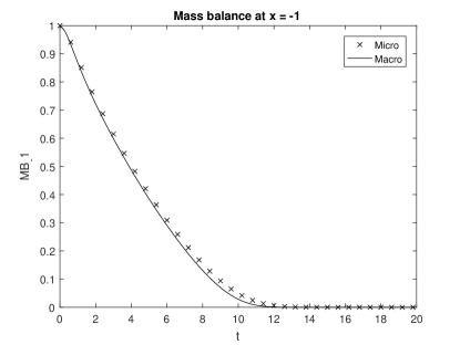
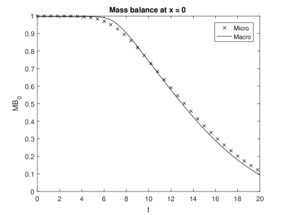
MBx^(u(t,)):=(,x^]×u(t,x)𝑑xassignsubscriptMB^𝑥𝑢𝑡subscript^𝑥𝑢𝑡𝑥differential-d𝑥\displaystyle\operatorname{MB}_{\hat{x}}(u(t,\cdot)):=\int_{(-\infty,\hat{x}]\times\R}u(t,x)dx (4.2)

at some vertical cut at position x^^𝑥absent\hat{x}\in\R determines the amount of mass in front of the cut. This measure extracts information about the time needed that a certain percentage of pedestrians crossed the cut.

In the following examples, we assume that the destination force is a point force

D(x)=xDxxDx𝐷𝑥superscript𝑥𝐷𝑥normsuperscript𝑥𝐷𝑥D(x)=\frac{x^{D}-x}{||x^{D}-x||}

with destination point xD2x^{D}\in{}^{2} and interaction kernel G𝐺G as the gradient of a Morse Potential, i.e.

G(x)=2(e(x0.9)e2(x0.9))xx.𝐺𝑥2superscript𝑒norm𝑥0.9superscript𝑒2norm𝑥0.9𝑥norm𝑥G(x)=-2(e^{-(||x||-0.9)}-e^{-2(||x||-0.9)})\frac{x}{||x||}.

The microscopic model is only comparable to the macroscopic one if we assume that the initial velocities are given by the closure velocities of the macroscopic model, i.e., for randomly generated positions (x1,,xN)subscript𝑥1subscript𝑥𝑁(x_{1},\dots,x_{N}) and states (r1,,rN)subscript𝑟1subscript𝑟𝑁(r_{1},\dots,r_{N}), we set

vi=riτ1+τλ(1,xi)(vCτD(xi)+1Nj=1NG(xixj)),subscript𝑣𝑖subscript𝑟𝑖𝜏1𝜏𝜆1subscript𝑥𝑖superscript𝑣𝐶𝜏𝐷subscript𝑥𝑖1𝑁superscriptsubscript𝑗1𝑁𝐺subscript𝑥𝑖subscript𝑥𝑗v_{i}=r_{i}\frac{\tau}{1+\tau\lambda(1,x_{i})}\left(\frac{v^{C}}{\tau}D(x_{i})+\frac{1}{N}\sum_{j=1}^{N}G(x_{i}-x_{j})\right),

where the initial states risubscript𝑟𝑖r_{i} are computed according to a Bernoulli distribution with initial probability P(ri=0)=p0[0,1]𝑃subscript𝑟𝑖0subscript𝑝001P(r_{i}=0)=p_{0}\in[0,1].

Example 1: Corridor with Space Dependent Rates

As a first example, we consider a strip without obstacles with boundaries given by bold lines, see figure 4. The comfort velocity vCsuperscript𝑣𝐶v^{C} and the relaxation time τ𝜏\tau are assumed to be one. The distribution of the initial positions should be

ρ0(B)=12B𝟙[2,1]×[1,1](x,y)d(x,y).superscript𝜌0𝐵12subscript𝐵subscript12111𝑥𝑦𝑑𝑥𝑦\rho^{0}(B)=\frac{1}{2}\int_{B}\mathds{1}_{[-2,-1]\times[-1,1]}(x,y)d(x,y).

Additionally, the initial conditions for the macroscopic model are

g0(x,y)=p0𝟙[2,1]×[1,1](x,y) and g1(x,y)=(1p0)𝟙[2,1]×[1,1](x,y)subscript𝑔0𝑥𝑦subscript𝑝0subscript12111𝑥𝑦 and subscript𝑔1𝑥𝑦1subscript𝑝0subscript12111𝑥𝑦g_{0}(x,y)=p_{0}\mathds{1}_{[-2,-1]\times[-1,1]}(x,y)\text{ and }g_{1}(x,y)=(1-p_{0})\mathds{1}_{[-2,-1]\times[-1,1]}(x,y)

supplemented by the initial probability to stop p0=12subscript𝑝012p_{0}=\frac{1}{2}.

We are interested in the dynamic behavior of the model for a space dependent rate function:

λ(0,x)𝜆0𝑥\displaystyle\lambda(0,x) ={6 if x0.510 else,absentcases6 if norm𝑥0.510 else,\displaystyle=\begin{cases}6&\text{ if }||x||\leq 0.5\\ 10&\text{ else,}\end{cases} (4.3)
λ(1,x)𝜆1𝑥\displaystyle\lambda(1,x) ={5 if x0.54 else.absentcases5 if norm𝑥0.54 else.\displaystyle=\begin{cases}5&\text{ if }||x||\leq 0.5\\ 4&\text{ else.}\end{cases} (4.4)

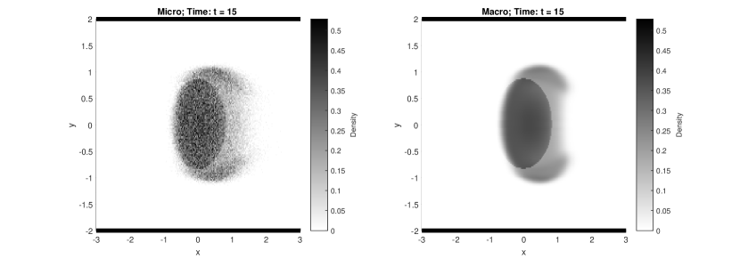
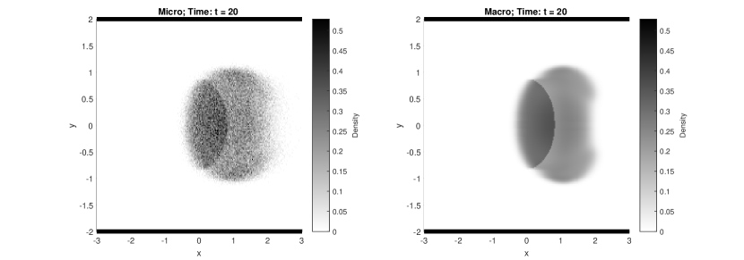
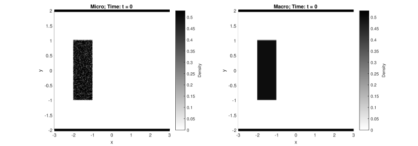
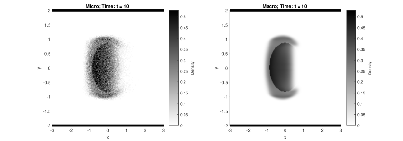
The results of a simulation with destination xD=(100,0)superscript𝑥𝐷1000x^{D}=(100,0), Δx=Δy=140Δ𝑥Δ𝑦140\Delta x=\Delta y=\frac{1}{40}, N=100𝑁100N=100 pedestrians and M=1000𝑀1000M=1000 Monte Carlo iterations are shown in figure 4. For our computations, we have used a WIN10 operated PC with 4-core i5-4690 CPU 3.50GHz, 16GB DDR3 RAM. All codes are implemented in MATLAB R2016b. The computation times we observed are 5149 seconds for the microscopic and 434 seconds for the macroscopic model.

In this scenario, the rate λ𝜆\lambda describes the number of events per time such that equations (4.3) and (4.4) indicate that pedestrians will stop more frequently than intend to walk inside the circle around the origin with radius 0.50.50.5. We expect that walking pedestrians circulate around the non-moving crowd and merge behind the bulk until a comfort density is reached again, cf. times t=10𝑡10t=10 and t=15𝑡15t=15 in figure 4. As we can also see, the influence of the space dependent rate on the density is significant since the density is much higher in the region where people stop longer and walk shorter.
Refer to caption
(a)
Refer to caption
(b)
Refer to caption
(c)
Refer to caption
(d)
Figure 4: Densities at different times

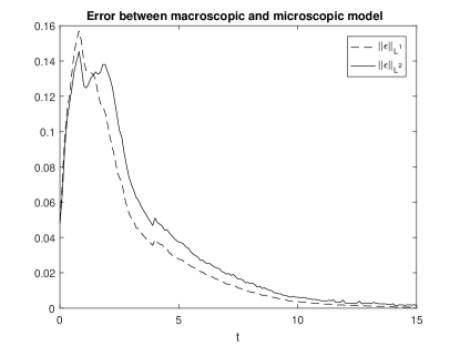
Apparently, the results from the microscopic and the macroscopic simulation are quite close, i.e. the density profiles show the same qualitative behavior in time. This can be also verified by the mass balance in figure 5 and the L1superscript𝐿1L^{1} and L2superscript𝐿2L^{2} error in figure 6.

Refer to caption
(a)
Refer to caption
(b)
Figure 5: Mass balances at x=1𝑥1x=-1 and x=0𝑥0x=0
Refer to caption
Figure 6: L1superscript𝐿1L^{1} and L2superscript𝐿2L^{2} error

Example 2: Corridor including Bottlenecks

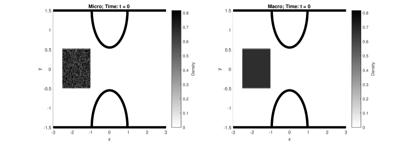
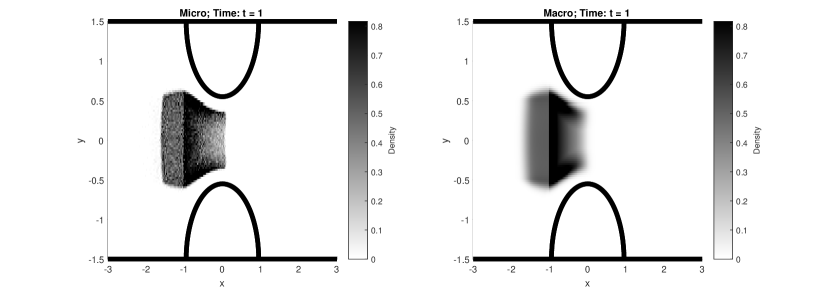
Different to the first example, we now focus on a scenario where two obstacles are located oppositely, see bold boundaries in figures 7 and 8. We distinguish the rate functions λ1subscript𝜆1\lambda_{1} and λ2subscript𝜆2\lambda_{2} to basically cover two relevant scenarios:

λ1(0,x)subscript𝜆10𝑥\displaystyle\lambda_{1}(0,x) ={1 if x[1,1],10 else,absentcases1 if 𝑥1110 else,\displaystyle=\begin{cases}1&\text{ if }x\in[-1,1],\\ 10&\text{ else,}\end{cases} λ1(1,x)subscript𝜆11𝑥\displaystyle\lambda_{1}(1,x) ={1 if x[1,1],1100 else,absentcases1 if 𝑥111100 else,\displaystyle=\begin{cases}1&\text{ if }x\in[-1,1],\\ \frac{1}{100}&\text{ else,}\end{cases}
λ2(0,x)subscript𝜆20𝑥\displaystyle\lambda_{2}(0,x) =10,absent10\displaystyle=10, λ2(1,x)subscript𝜆21𝑥\displaystyle\lambda_{2}(1,x) =1100.absent1100\displaystyle=\frac{1}{100}.

The rate function λ1subscript𝜆1\lambda_{1} is in-homogeneous in space and divided into two cases. In the case x[1,1]𝑥11x\in[-1,1] which is exactly between the obstacles (e.g. external attractions) pedestrians will stop more often and stay for a longer period. Otherwise, for x(,1)(1,)𝑥11x\in(-\infty,-1)\cup(1,\infty), pedestrians behave deterministic since the scaling factor (1+τλ(1,x))1superscript1𝜏𝜆1𝑥1(1+\tau\lambda(1,x))^{-1} in (2.25) becomes very close to one and we get a velocity which corresponds to the deterministic model, cf. left column in figure 3. On the contrary, the rate function λ2subscript𝜆2\lambda_{2} is homogeneous in space but will be used as the deterministic benchmark problem, see again figure 3.

We consider the following setup: The destination is again located at xD=(100,0)superscript𝑥𝐷1000x^{D}=(100,0), the comfort speed is vC=1superscript𝑣𝐶1v^{C}=1 and the relaxation time is supposed to be τ=0.2𝜏0.2\tau=0.2. The initial distribution is

ρ0(B)=23B𝟙[2.5,1]×[0.5,0.5](x,y)d(x,y).superscript𝜌0𝐵23subscript𝐵subscript12.510.50.5𝑥𝑦𝑑𝑥𝑦\rho^{0}(B)=\frac{2}{3}\int_{B}\mathds{1}_{[-2.5,-1]\times[-0.5,0.5]}(x,y)d(x,y).

with probability p0=0.01subscript𝑝00.01p_{0}=0.01 to stop in the beginning. Therefore, the initial conditions for the macroscopic model read

g0(x,y)=p023𝟙[2.5,1]×[0.5,0.5](x,y) and g1(x,y)=(1p0)23𝟙[2.5,1]×[0.5,0.5](x,y).subscript𝑔0𝑥𝑦subscript𝑝023subscript12.510.50.5𝑥𝑦 and subscript𝑔1𝑥𝑦1subscript𝑝023subscript12.510.50.5𝑥𝑦g_{0}(x,y)=p_{0}\frac{2}{3}\mathds{1}_{[-2.5,-1]\times[-0.5,0.5]}(x,y)\text{ and }g_{1}(x,y)=(1-p_{0})\frac{2}{3}\mathds{1}_{[-2.5,-1]\times[-0.5,0.5]}(x,y).

The simulation is performed with step-sizes Δx=Δy=140Δ𝑥Δ𝑦140\Delta x=\Delta y=\frac{1}{40}, N=100𝑁100N=100 pedestrians and M=1000𝑀1000M=1000 Monte-Carlo iterations. We have used the same PC as before and the required computation times are 3006 seconds (λ1subscript𝜆1\lambda_{1}), 3205 seconds (λ2subscript𝜆2\lambda_{2}) for the microscopic model and 485 seconds (λ1subscript𝜆1\lambda_{1}), 495 seconds (λ2subscript𝜆2\lambda_{2}) for the macroscopic model.

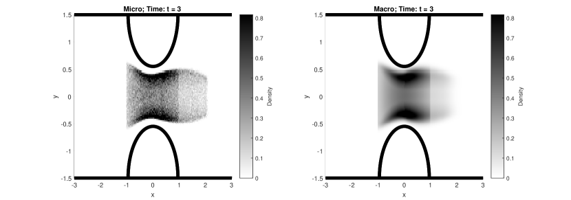
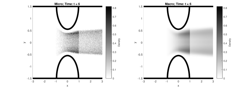
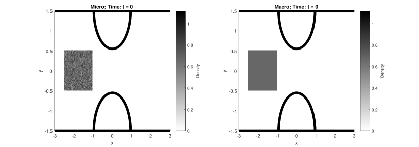
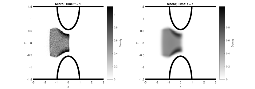
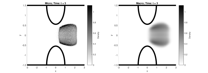
In figures 78 we plot the densities for different rate functions. The specular reflection type boundaries seem to work well and the pedestrians are rerouted along the obstacles. For the choice of λ1subscript𝜆1\lambda_{1} in figure 7, where the pedestrians tend to stop between the obstacles, we observe the expected queuing behavior. In contrast for the deterministic setting λ2subscript𝜆2\lambda_{2}, higher densities in front of the obstacles result from the spatial conditions only and are not caused by stop-or-go decisions, cf. figure 8.

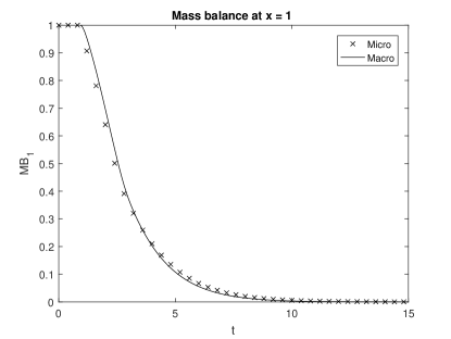
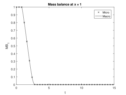
The influence of different rate functions is also reflected by the comparison of the mass balances in figure 9. The first scenario, the bottleneck situation, reduces significantly the mean velocity of the pedestrians and hence leads to longer travel times, see left picture in figure 9. After approximately 14 time units all pedestrians crossed the cut at x=1𝑥1x=1 while for the deterministic scenario only 2.5 time units are needed, cf. right picture in figure 9.

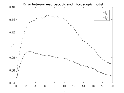
Finally, we stress that the error between the microscopic and macroscopic model is again rather small, as figure 10 illustrates, and is not affected by the different rate functions.
Refer to caption
(a)
Refer to caption
(b)
Refer to caption
(c)
Refer to caption
(d)
Figure 7: Densities for λ1subscript𝜆1\lambda_{1} at different times
Refer to caption
(a)
Refer to caption
(b)
Refer to caption
(c)
Figure 8: Densities for λ2subscript𝜆2\lambda_{2} at different times
Refer to caption
(a) Mass balance with λ1subscript𝜆1\lambda_{1}
Refer to caption
(b) Mass balance with λ2subscript𝜆2\lambda_{2}
Figure 9: Mass balances at x=1𝑥1x=1
Refer to caption
(a) Errors with λ1subscript𝜆1\lambda_{1}
Refer to caption
(b) Errors with λ2subscript𝜆2\lambda_{2}
Figure 10: L1superscript𝐿1L^{1} and L2superscript𝐿2L^{2} errors

Conclusion

We have introduced a stochastic microscopic pedestrian model with specular reflection type boundary conditions and proved its existence. Based on the microscopic model, we have derived a kinetic formulation under a mean field assumption in terms of measures. A non-standard closure assumption has been established to extract a first order macroscopic model given by a system of conservation laws. Numerical comparisons of the microscopic and macroscopic pedestrian flow model have been performed to demonstrate the same dynamical behavior for both modeling approaches.

Future work might include the investigation of a stochastic model hierarchy, where the Eikonal equation (instead of the destination force) is used to determine the shortest travel time to the desired destination, see [10]. The derivation of a second order macroscopic model seems to be also very appealing in this context.

Acknowledgments

This work was financially supported by the DAAD project “DAAD-PPP VR China” (project ID: 57215936) and the DFG grant GO 1920/4-1.

References

  • [1] D. Armbruster, S. Martin, and A. Thatcher, Elastic and inelastic collisions of swarms, Physica D: Nonlinear Phenomena, 344 (2017), pp. 45 – 57.
  • [2] D. Armbruster, S. Motsch, and A. Thatcher, Swarming in bounded domains, Physica D: Nonlinear Phenomena, 344 (2017), pp. 58 – 67.
  • [3] H. Bauer, Probability theory, vol. 23 of De Gruyter Studies in Mathematics, Walter de Gruyter & Co., Berlin, 1996. Translated from the fourth (1991) German edition by Robert B. Burckel and revised by the author.
  • [4] N. Bellomo, C. Bianca, and V. Coscia, On the modeling of crowd dynamics: an overview and research perspectives, See\vec{\rm e}MA J., (2011), pp. 25–46.
  • [5] C. Cercignani, R. Illner, and M. Pulvirenti, The mathematical theory of dilute gases, vol. 106 of Applied Mathematical Sciences, Springer-Verlag, New York, 1994.
  • [6] L. Chen, S. Göttlich, and Q. Yin, Mean field limit and propagation of chaos for a pedestrian flow model, Journal of Statistical Physics, 166 (2017), pp. 211–229.
  • [7] P. Degond, C. Appert-Rolland, M. Moussaïd, J. Pettré, and G. Theraulaz, A hierarchy of heuristic-based models of crowd dynamics, J. Stat. Phys., 152 (2013), pp. 1033–1068.
  • [8] P. Degond, C. Appert-Rolland, J. Pettré, and G. Theraulaz, Vision-based macroscopic pedestrian models, Kinet. Relat. Models, 6 (2013), pp. 809–839.
  • [9] P. Degond and C. Ringhofer, Stochastic dynamics of long supply chains with random breakdowns, SIAM J. Appl. Math., 68 (2007), pp. 59–79.
  • [10] R. Etikyala, S. Göttlich, A. Klar, and S. Tiwari, Particle methods for pedestrian flow models: from microscopic to nonlocal continuum models, Math. Models Methods Appl. Sci., 24 (2014), pp. 2503–2523.
  • [11] I. I. Gikhman and A. V. Skorokhod, The theory of stochastic processes. II, Classics in Mathematics, Springer-Verlag, Berlin, 2004. Translated from the Russian by S. Kotz, Reprint of the 1975 edition.
  • [12] D. Helbing, A fluid dynamic model for the movement of pedestrians, Complex Systems 6, 391-415, (1992).
  • [13] D. Helbing and P. Molnár, Social force model for pedestrian dynamics, Physical Review E 51, 4282-4286, (1995).
  • [14] R. L. Hughes, A continuum theory for the flow of pedestrians, Transportation Research Part B: Methodological, 36 (2002), pp. 507–535.
  • [15] P.-E. Jabin, Macroscopic limit of Vlasov type equations with friction, Ann. Inst. H. Poincaré Anal. Non Linéaire, 17 (2000), pp. 651–672.
  • [16] P.-E. Jabin, Various levels of models for aerosols, Mathematical Models and Methods in Applied Sciences, 12 (2002), pp. 903–919.
  • [17] A. Jüngel, Transport equations for semiconductors, vol. 773 of Lecture Notes in Physics, Springer-Verlag, Berlin, 2009.
  • [18] A. Klar, F. Schneider, and O. Tse, Approximate models for stochastic dynamic systems with velocities on the sphere and associated fokker–planck equations, Kinetic and Related Models, 7 (2014), pp. 509–529.
  • [19] R. J. LeVeque, Finite volume methods for hyperbolic problems, Cambridge Texts in Applied Mathematics, Cambridge University Press, Cambridge, 2002.
  • [20] B. Piccoli and A. Tosin, Pedestrian flows in bounded domains with obstacles, Contin. Mech. Thermodyn., 21(2):85-107, (2009).
  • [21] B. Piccoli and A. Tosin, Time-evolving measures and macroscopic modeling of pedestrian flow, Arch. Ration. Mech. Anal., 199(3):707-738, (2011).