A Numerical Method for Pricing Discrete Double Barrier Option by Legendre Multiwavelet

Abstract

In this Article, a fast numerical numerical algorithm for pricing discrete double barrier option is presented. According to Black-Scholes model, the price of option in each monitoring date can be evaluated by a recursive formula upon the heat equation solution. These recursive solutions are approximated by using Legendre multiwavelets as orthonormal basis functions and expressed in operational matrix form. The most important feature of this method is that its CPU time is nearly invariant when monitoring dates increase. Besides, the rate of convergence of presented algorithm was obtained. The numerical results verify the validity and efficiency of the numerical method.

1 Introduction

Barrier options play a key role in the price risk management of financial markets. There are two types of barrier options: single and double. In single case we have one barrier but in double case there are two barriers. A barrier option is called knock-out (knock-in) if it is deactivated (activated) when the stock price touches one of the barriers. If the hitting of barriers by the stock price is checked in fixed dates, for example weakly or monthly, the barrier option is called discrete.

Option pricing as one of the most interesting topics in the mathematical finance has been investigated vastly in the literature. Kamrad and Ritchken [1], Boyle and Lau [2], Kwok [3], Heyen and Kat [4], Tian [5] and Dai and Lyuu [6] used standard lattice techniques, the binomial and trinomial trees, for pricing barrier options. Ahn et al. [7] introduce the adaptive mesh model (AMM) that increases the efficiency of trinomial lattices. The Monte Carlo simulation methods were implemented in [8, 9, 10, 11, 12]. In [13, 14], numerical algorithms based on quadrature methods were proposed.

Actually a great variety of semi-analytical methods to price barrier options have been recently developed which are based on integral transforms [15, 16, 17], or on the transition probability density function of the process used to describe the underlying asset price [13, 14, 18, 19, 20, 21, 22, 23]. These techniques are very high performing for pricing discretely monitored one and double barrier options and our computational results are in very good agreement with them. We would like to make the following essential remarks. An analytical solution for single barrier option is driven by Fusai et. al. in [15] where the problem of one barrier is reduced to a Wiener-Hopf integral equation and a given z-transform solution of it. To derive a formula for continuous double barrier knock-out and knock-in options Pelsser inverts analytically the Laplace transform by a contour integration [24]. Broadie et. al. have found an explicit correction formula for discretely monitored option with one barrier [19]. However, these three well-known methods [15, 19, 24] have not been still applied in the presence of two barriers, i.e. a discrete double barrier option. Farnoosh et al. [25, 26] presented numerical algorithms for pricing discrete single and double barrier options with time-dependent parameters. Also, in my last work [27] a numerical method for pricing discrete single and double barrier options by projection methods have been presented.

This article is organized as follows. In Section 2, the process of finding price of discrete double barrier option under the Black-Scholes model by a recursive formula has bean explained. Definition and some features of Legendre multi-wavelets are given in section 3. In section 4, Legendre multi-wavelet expansion is implemented for pricing of discrete double barrier option. Finally, numerical results are given in section 5 to confirm efficiency of proposed method.

2 The Pricing Model

We assume that the stock price process follows geometric Brownian motion:

$$d{S_{t}}=\hat{r}{S_{t}}dt+\sigma{S_{t}}d{B_{t}}$$

where ${S_{0}}$, $\hat{r}$ and $\sigma$ are initial stock price, risk-free rate and volatility respectively. We consider the problem of pricing knock-out discrete double barrier call option, i.e. a call option that becomes worthless if the stock price touches either lower or upper barrier at the predetermined monitoring dates:

$$0={t_{0}}<{t_{1}}<\cdots<{t_{M}}=T.$$

If the barriers are not touched in monitoring dates, the pay off at maturity time is $max(S_{T}-E,0)$, where $E$ is exercise price. The price of option is defined discounted expectation of pay off at the maturity time.

Based on Black-Scholes framework, the option price $\mathcal{P}\left({S,t,m-1}\right)$ as a function of stock price at time $t\in\left({{t_{m-1}},{t_{m}}}\right)$, satisfies in the following partial differential equations[28]

$$-\frac{{\partial\mathcal{P}}}{{\partial t}}+\hat{r}S\frac{{\partial\mathcal{P}}}{{\partial S}}+\frac{1}{2}{\sigma^{2}}{S^{2}}\frac{{{\partial^{2}}\mathcal{P}}}{{\partial{S^{2}}}}-\hat{r}\mathcal{P}=0,$$ (1)

subject to the initial conditions:

$$\mathcal{P}\left({S,{t_{0}},0}\right)=\left({S-E}\right){\textbf{1}_{\left(\max(E,L)\leq S\leq U\right)}}\,$$

$$\mathcal{P}\left({S,{t_{m}},0}\right)=\mathcal{P}\left({S,{t_{m}},m-1}\right){\textbf{1}_{\left(L\leq S\leq U\right)}};\,\,m=1,2,...,M-1~{},$$

where $\mathcal{P}\left({S,{t_{m}},m-1}\right):=\mathop{\lim}\limits_{t\to{t_{m}}}\mathcal{P}\left({S,t,m-1}\right)$. By change of variable $z=\ln\left({\frac{S}{L}}\right)$ the partial differential equation 1 and its initial condition is reduced as follows:

$$-{C_{t}}+\mu{C_{z}}+\frac{{{\sigma^{2}}}}{2}{C_{zz}}=\hat{r}C$$ (2)

$$C\left({z,{t_{0}},0}\right)=L\left({{e^{z}}-{e^{{E^{*}}}}}\right){\textbf{1}_{\left(\delta\leq z\leq\theta\right)}}$$

$$C\left({z,{t_{m}},m}\right)=C\left({z,{t_{m}},m-1}\right){\textbf{1}_{\left(0\leq z\leq\theta\right)}}\,;\,\,m=1,2,...,M-1\,\,$$

where $C(z,t,m):=\mathcal{P}(S,t,m);\,{E^{*}}=\ln\left({\frac{E}{L}}\right);\,\mu=\hat{r}-\frac{{{\sigma^{2}}}}{2};\,\theta=\ln\left({\frac{U}{L}}\right)$ and $\delta=\max\left\{{{E^{*}},0}\right\}$. Next, by considering $C\left({z,{t_{m}},m}\right)={e^{\alpha z+\beta t}}h(z,t,m)$ where:

$$\alpha=-\frac{\mu}{{{\sigma^{2}}}};\,\,{c^{2}}=-\frac{{{\sigma^{2}}}}{2};\,\beta=\alpha\mu+{\alpha^{2}}\frac{{{\sigma^{2}}}}{2}-\hat{r}.$$

the equation 2 is reduced to the well known heat equation:

$$-{h_{t}}+{c^{2}}{h_{zz}}=0$$

$$h\left({z,{t_{0}},0}\right)=L{e^{-\alpha z}}\left({{e^{z}}-{e^{{E^{*}}}}}\right){\textbf{1}_{\left(\delta\leq z\leq\theta\right)}};\,m=0$$

$$h\left({z,{t_{m}},m}\right)=h\left({z,{t_{m}},m-1}\right){\textbf{1}_{\left(0\leq\theta\leq z\right)}};\,m=1,...,M-1$$

that could be resolved analytically, see e.g [29] as follows;

$$h(z,t,m)=\left\{\begin{array}[]{l}L\int_{\delta}^{\theta}{{k}\left({z-\xi,t}\right){e^{-\alpha\xi}}\left({{e^{\xi}}-{e^{{E^{*}}}}}\right)d\xi\,;\,\,m=0}\\ \int_{0}^{\theta}{k\left({z-\xi,t-{t_{m}}}\right)h\left({\xi,{t_{m}},m-1}\right)d\xi}\,;\,\,m=1,2,...,M-1\end{array}\right.$$

where

$$\overline{k}(z,t)=\frac{1}{{\sqrt{4\pi{c^{2}}t}}}{e^{-\frac{{{z^{2}}}}{{4{c^{2}}t}}}}.$$ (3)

By assuming that monitoring dates are equally spaced, i.e; ${t_{m}}=m\tau$ where $\tau=\frac{T}{M}$, $h\left({z,{t_{m}},m-1}\right)$ is a function of two variables $z$, $m$. Therefore, by defining ${\overline{f}_{m}}\left(z\right):=h(z,{t_{m}},m-1)$, we have:

$${\overline{f}_{1}}(z)=\int_{0}^{\theta}{\overline{k}(z-\xi,\tau){\overline{f}_{0}}\left(\xi\right)d\xi}$$ (4)

$${\overline{f}_{m}}(z)=\int_{0}^{\theta}{\overline{k}(z-\xi,\tau){\overline{f}_{m-1}}\left(\xi\right)d\xi};\,m=2,3,...,M$$ (5)

where

$$\overline{f}_{0}\left(z\right)=L{e^{-\alpha z}}\left({{e^{z}}-{e^{{E^{*}}}}}\right){\textbf{1}_{\left(\delta\leq z\leq\theta\right)}}.$$ (6)

by defining $f_{m}(z):=\overline{f}_{m}(\theta z)$ and

$$k(z,\tau):=\theta\overline{k}(\theta z,\tau)=\frac{1}{{\sqrt{4\pi{c^{2}}t}}}{e^{-\frac{{{(\theta z)^{2}}}}{{4{c^{2}}t}}}}$$ (7)

we reach the following relations from 4,5 and 6:

$${f}_{1}(z)=\int_{0}^{1}{k(z-\xi,\tau){f_{0}}\left(\xi\right)d\xi}$$ (8)

$${f_{m}}(z)=\int_{0}^{1}{k(z-\xi,\tau){f_{m-1}}\left(\xi\right)d\xi};\,m=2,3,...,M$$ (9)

where

$$f_{0}\left(z\right)=L{e^{-\alpha\theta z}}\left({{e^{\theta z}}-{e^{{E^{*}}}}}\right){\textbf{1}_{\left(\frac{\delta}{\theta}\leq z\leq 1\right)}}.$$ (10)

which helps us to use Legendre multiwavelete on interval $[0,1]$.

3 Legendre Multiwavelet

Let $L^{2}([0,1])$ be the Hilbert space of all square-integrable functions on interval $[0,1]$ with the inner product

$$<f,g>:=\int_{0}^{1}f(x)g(x)dx$$

and the norm $\|f\|=\sqrt{<f,f>}$. An orthonormal multi resolution analysis (MRA) with multiplicity $r$ of $L^{2}([0,1])$ is defined as follows:

Definition 1.

A chain of closed functional subspaces $V_{j},j\geq 0$ of $L^{2}([0,1])$ is called orthonormal multi resolution analysis of multiplicity $r$ if:

1. $V_{j}\subset V_{j+1},j\geq 0$.

2. $\bigcup\limits_{j\geq 0}V_{j}$ is dense in $L^{2}([0,1])$,i.e.$\overline{\bigcup\limits_{j\geq 0}V_{j}}=L^{2}([0,1])$.

3. There exists a vector of orthonormal functions $\Phi=[\phi^{0},...,\phi^{r-1}]^{T}$ in $L^{2}([0,1])$, that is called multiscale vector, such that $\{\phi^{l}_{j,k}:=2^{j/2}\phi^{l}(2^{j}x-k);0\leq l\leq r-1,0\leq k\leq 2^{j}-1\}$ form an orthonormal basis for $V_{j}$.

Now let wavelet space $W_{j}$ be subspace of $V_{j+1}$ such that $V_{j+1}=V{j}\oplus W_{j}$ and $V{j}\perp W_{j}$, i.e. the orthogonal complement of $V_{j}$ in $V_{j+1}$, so we have

$$V_{j}=V_{0}\oplus W_{0}\oplus W_{1}\oplus...W_{j-1}$$ (11)

$$L^{2}([0,1])=V0\oplus\bigoplus\limits_{j=0}^{\infty}W_{j}.$$ (12)

The property3 of MRA shows that $dim(V_{j})=dim(W_{j})=r2^{j}$. Let the function vector $\Psi=[\psi^{0},...,\psi^{r-1}]$ be vector of orthonormal basis of $W_{0}$, that is called multiwavelet vector, then the structure of MRA implies that

$$W_{j}=\overline{span\{\psi^{l}_{j,k};0\leq l\leq r-1,0\leq k\leq 2^{j}-1\}},$$ (13)

where $\psi^{l}_{j,k}:=2^{j/2}\psi^{l}(2^{j}x-k)$. According to 3 and 11 for any $V_{j}$ we have two orthonormal basis set as follow:

$$\Phi_{j}(x)=[\phi_{j,0}^{0}(x),...,\phi_{j,0}^{r-1}(x),...,\phi_{j,2^{j}-1}^{0}(x),...,\phi_{j,2^{j}-1}^{r-1}(x)]$$ (14)

$$\Psi_{j}(x)=[\phi_{0,0}^{0}(x),...,\phi_{0,0}^{r-1}(x),\psi_{0,0}^{0}(x),...,\psi_{0,0}^{r-1}(x),...,\\ \psi_{j-1,0}^{0}(x),...,\psi_{j-1,0}^{r-1}(x),...,\psi_{j-1,2^{j-1}-1}^{0}(x),...,\psi_{j-1,2^{j-1}-1}^{r-1}(x)]$$ (15)

From relation 12 for any $f\in L^{2}([0,1])$ we have

$$f(x)=\sum_{l=0}^{r-1}c_{l}\phi^{l}(x)+\sum_{j=0}^{\infty}\sum_{k=0}^{2^{j-1}}\sum_{l=0}^{r-1}c_{j,k}\psi_{j,k}^{l}(x)$$ (16)

where $c_{l}=\int_{0}^{1}f(x)\phi^{l}(x)dx$ and $c_{j,k}=\int_{0}^{1}f(x)\psi_{j,k}^{l}(x)dx$.
Now we define orthonormal projection operator $P_{J}:L^{2}([0,1])\rightarrow V_{J}$ as follows:

$$P_{J}(f):=\sum_{l=0}^{r-1}c_{l}\phi^{l}(x)+\sum_{j=0}^{J-1}\sum_{k=0}^{2^{j-1}}\sum_{l=0}^{r-1}c_{j,k}\psi_{j,k}^{l}(x)$$ (17)

or equivalently

$$P_{J}(f):=\sum_{k=0}^{2^{J}}\sum_{l=0}^{r-1}d_{J,k}\phi_{J,k}^{l}(x)$$ (18)

where $d_{j,k}=\int_{0}^{1}f(x)\phi_{j,k}^{l}(x)dx$. In order to simplify notation, we denote the i-th element of $\Psi_{j}(x)$ by $\overline{\psi}_{i}(x)$, so:

$$\Psi_{j}(x)=[\overline{\psi}_{1}(x),\overline{\psi}_{2}(x),...,\overline{\psi}_{2^{j}}(x)]$$ (19)

and then we can rewrite 17:

$$P_{J}(f):=\sum_{i=0}^{2^{J}}a_{i}\overline{\psi}_{i}(x)=\Psi_{j}(x)^{\prime}F$$ (20)

where $a_{i}=\int_{0}^{1}f(x)\overline{\psi}_{i}(x)dx$ and $F=[a_{1},...,a_{2^{j}}]$. From relation 16 $P_{J}$ is convergence pointwise to identity operator $I$, i.e.

$$\forall f\in L^{2}[0,\theta]~{}~{}~{}\mathop{\lim}\limits_{J\to\infty}\left\|{{P_{J}}(f)-f}\right\|=0.$$ (21)

We use Legendre polynomial to construct Legendre Multiwavelet that has introduced by Alpert in [30]. Legendre polynomial, ${p_{i}}(x)$, is defined as follows

$${p_{0}}(x)=1\,\,\,\,,\,\,\,{p_{1}}(x)=x$$

with the following recurrence formula:

$${p_{i}}(x)=x{p_{i-1}}(x)+\left({\frac{i}{{i+1}}}\right)\left({x{p_{i-1}}(x)-{p_{i-2}}(x)}\right)$$

The $\left\{{{p_{i}}(x)}\right\}_{i=0}^{\infty}$ is an orthogonal basis for ${L^{2}}([-1,1])$.
We define $V_{j}$ as follows

$$V_{j}:=\{f|~{}f~{}be~{}a~{}polynomial~{}of~{}degree\leq r~{}on~{}I_{i},1\leq i\leq 2^{j}\}$$ (22)

where $I_{i}:=[2^{-j}(i-1),2^{-j}i)$. It is obvious that $V_{j}\subset V_{j+1}$ and $\overline{\bigcup\limits_{j\geq 0}V_{j}}=L^{2}([0,1])$. Now let $\phi^{l}$ be a Legendre multiscaling function, that is defined as

$$\phi^{l}:=\left\{\begin{array}[]{ll}\sqrt{2l+1}p_{l}(2x-1)&x\in[0,1),\\ 0,&o.w,\end{array}\right.$$ (23)

and $\Phi:=[\phi^{0},...,\phi^{r-1}]^{T}$ be the multiscale vector. It is easy to verify that

$$\{\phi^{l}_{j,k}:=2^{j/2}\phi^{l}(2^{j}x-k);0\leq l\leq r-1,0\leq k\leq 2^{j}-1\},$$ (24)

forms an orthonormal basis for $V_{j}$. Now let $\Psi=[\psi^{1},...,\psi^{r-1}]$ be the Legendre multiwavelet vector. Because of $W_{0}\subset V_{1}$ each $\psi_{l}$ could be expanded as follows:

$$\psi^{l}=\sum_{k=0}^{r-1}g_{l,k}^{0}\phi^{k}(2x)+\sum_{k=0}^{r-1}g_{l,k}^{1}\phi^{k}(2x-1)~{}~{},~{}~{}0\leq l\leq r-1$$ (25)

In addition, $W_{0}\perp V_{0}$ and $1,x,..,x^{r-1}\in V_{0}$, so the first $r$ moment of $\{\psi^{l}\}_{l=0}^{r-1}$ vanish:

$$\int_{0}^{1}\psi^{l}(x)x^{i}dx=0~{}~{}~{}0\leq l,i\leq r-1$$ (26)

on the other hand, we have

$$\int_{0}^{1}\psi^{i}(x)\psi^{j}(x)dx=0~{}~{}~{}0\leq i,j\leq r-1$$ (27)

so for finding $2r^{2}$ unknown coefficients $g_{i,j}$ in 25, it is enough to solve $2r^{2}$ equations 26 and 27. If $f\in L^{2}([0,1])$ be $k$ times differentiable, the following theorem about bound of error is obtained [30]:

Theorem 1.

Suppose that the real function $f\in C^{r}([0,1])$. Then $P_{J}(f)$ approximates $f$ with the following error bound:

$$\|P_{J}(f)-f\|\leq\frac{2^{(-Jr+1)}}{4^{r}r!}\sup_{x\in[0,1]}|f^{r}(x)|.$$ (28)

Legendre multiscaling and multiwavelet functions are presented for $r=4$ as follows [31]:

$$\begin{array}[]{l r }\phi^{0}(x)=1&0\leq x<1\\ \phi^{1}(x)=\sqrt{3}\left(2\,x-1\right)&0\leq x<1\\ \phi^{2}(x)=\sqrt{5}\left(6\,{x}^{2}-6\,x+1\right)&0\leq x<1\\ \phi^{3}(x)=\sqrt{7}\left(20\,{x}^{3}-30\,{x}^{2}+12\,x-1\right)&0\leq x<1\end{array}$$ (29)

$$\begin{array}[]{l }\psi^{0}(x)=\begin{cases}-\sqrt{\frac{15}{34}}\left(224\,{x}^{3}-216\,{x}^{2}+56\,x-3\right)&0\leq x<1/2\\ \sqrt{\frac{15}{34}}\left(224\,{x}^{3}-456\,{x}^{2}+296\,x-61\right)&1/2\leq x<1/2\end{cases}\\ \vskip 6.0pt plus 2.0pt minus 2.0pt\cr\psi^{1}(x)=\begin{cases}-\sqrt{\frac{1}{21}}\left(1680\,{x}^{3}-1320\,{x}^{2}+270\,x-11\right)&0\leq x\leq 1/2\\ \sqrt{\frac{1}{21}}\left(1680\,{x}^{3}-3720\,{x}^{2}+2670\,x-619\right)&1/2\leq x<1/2\end{cases}\\ \vskip 6.0pt plus 2.0pt minus 2.0pt\cr\psi^{2}(x)=\begin{cases}-\sqrt{\frac{35}{17}}\left(256\,{x}^{3}-174\,{x}^{2}+30\,x-1\right)&0\leq x<1/2\\ \sqrt{\frac{35}{17}}\left(256\,{x}^{3}-594\,{x}^{2}+450\,x-111\right)&1/2\leq x<1/2\end{cases}\\ \vskip 6.0pt plus 2.0pt minus 2.0pt\cr\psi^{3}(x)=\begin{cases}\sqrt{\frac{5}{42}}\left(420\,{x}^{3}-246\,{x}^{2}+36\,x-1\right)&0\leq x<1/2\\ \sqrt{\frac{5}{42}}\left(420\,{x}^{3}-1014\,{x}^{2}+804\,x-209\right)&1/2\leq x<1/2\end{cases}\par\par\end{array}$$ (30)

4 Pricing by Legendre Multiwavelet

Let operator $\mathcal{K}:L^{2}([0,1])\to L^{2}([0,1])$ is defined as follows:

$$\mathcal{K}\left(f\right)(z):=\int_{0}^{1}{\kappa(z-\xi,\tau)f(\xi)}d\xi.$$ (31)

where $\kappa$ is defined in 7. Because $\kappa$ is a continuous function, $\mathcal{K}$ is a bounded linear compact operator on $L^{2}([0,1])$[32, 33]. According to the definition of operator $\mathcal{K}$, equations 8 and 9 can be rewritten as below:

$$f_{1}=\mathcal{K}f_{0}$$ (32)

$$f_{m}=\mathcal{K}f_{m-1}~{}~{}\,m=2,3,...,M$$ (33)

We denote

$${{\tilde{f}}_{1,J}}={P_{J}}\mathcal{K}\left({{f_{0}}}\right)$$ (34)

$${{\tilde{f}}_{m,J}}={P_{J}}\mathcal{K}\left({{{\tilde{f}}_{m-1,J}}}\right)=\left({P_{J}}\mathcal{K}\right)^{m}\left(f_{0}\right)\,,\,m\geq 2.$$ (35)

where ${P_{J}}\mathcal{K}$ is as follows:

$$({P_{J}}\mathcal{K})(f)={P_{J}}\left({\mathcal{K}(f)}\right).$$

Since the continuous projection operators ${P_{J}}$ converge pointwise to identity operator $I$, then operator ${P_{J}}\mathcal{K}$ is also a compact operator and

$$\mathop{\lim}\limits_{n\to\infty}\left\|{{P_{J}}\mathcal{K}-\mathcal{K}}\right\|=0$$ (36)

(see [34]). With attention to the following inequality

$$\left\|{\left({{P_{J}}\mathcal{K}}\right)}^{m}-{\mathcal{K}^{m}}\right\|\leq\|\left({{P_{J}}\mathcal{K}}\right)\|\|{\left({{P_{J}}\mathcal{K}}\right)}^{m-1}-{\mathcal{K}^{m-1}}\|-\|{{P_{J}}\mathcal{K}-\mathcal{K}}\|\|{\mathcal{K}}\|^{m-1}$$ (37)

and relation 36 by induction we get

$$\mathop{\lim}\limits_{n\to\infty}\left\|{\left({{P_{J}}\mathcal{K}}\right)}^{m}-{\mathcal{K}^{m}}\right\|=0.$$ (38)

Therefore, the following convergence result is concluded:

$$\left\|{{{\tilde{f}}_{m,J}}-{f_{m}}}\right\|=\left\|{\left({{P_{J}}\mathcal{K}}\right)}^{m}\left(f_{0}\right)-\mathcal{K}^{m}\left(f_{0}\right)\right\|\leq\left\|{{{\left({{P_{J}}\mathcal{K}}\right)}^{m}}-{\mathcal{K}^{m}}}\right\|\left\|{{f_{0}}}\right\|\to 0as\,\,J\to\infty.$$ (39)

From 37 and 39, we infer that the rate of convergence ${\tilde{f}}_{m,J}$ to ${f_{m}}$ and ${{P_{J}}\mathcal{K}}$ to $\mathcal{K}$ are the same. Using the relation 28 and properties of integral operator $\mathcal{K}$, it is easy to confirm that

$$\left\|{{P_{J}}\mathcal{K}-\mathcal{K}}\right\|\leq\frac{2^{(-Jr+1)}}{4^{r}r!}\sup_{z,\xi\in[0,1]}|\frac{\partial\kappa(z-\xi,\tau)}{\partial z^{r}}|.$$ (40)

Since, ${\tilde{f}_{m,J}}\in{V_{J}}$ for $m\geq 1$, we can write

$${\tilde{f}_{m,J}}=\sum\limits_{i=0}^{{r2^{J}}}{{a_{mi}}{\overline{\psi}_{i}}(z)}={\Psi^{\prime}_{J}}(x)F_{m},$$

where ${F_{m}}=[{a_{m0}},{a_{m1}},\cdots,{a_{m{2^{j}}}}]^{\prime}$. From equation 35 we obtain

$${\tilde{f}_{m,J}}={({P_{J}}\mathcal{K})^{m-1}}{\left(\tilde{f}_{1,J}\right)}.$$ (41)

Since ${V_{J}}$ is a finite dimensional linear space, thus the linear operator ${P_{J}}\mathcal{K}$ on ${V_{J}}$ could be considered as a ${r2^{J}}\times{r2^{J}}$ matrix $K$. Consequently equation 41 can be written as following matrix operator form

$${\tilde{f}_{m,J}}={\Psi^{\prime}_{J}}{K^{m-1}}{F_{1}}.$$ (42)

For evaluation of the option price by 42, it is enough to calculate the matrix operator $K$ and the vector ${F_{1}}$. It is easy to check (see [27]) that:

$${F_{1}}=[{a_{11}},{a_{12}},\cdots,{a_{1r2^{J}}}]^{\prime}$$

$$K={\left({{k_{ij}}}\right)_{{r2^{J}}\times{r2^{J}}}}$$

where

$${a_{1i}}=\int_{0}^{1}{\int_{\delta/\theta}^{1}{{\overline{\psi}_{i}}(\eta)\kappa(\eta-\xi,\tau){f_{0}}(\xi)d\xi d\eta}\,\,},\,\,0\leq i\leq r2^{J}.$$

$${k_{ij}}=\int_{0}^{1}{\int_{0}^{1}{{\overline{\psi}_{i}}(\eta){\overline{\psi}_{j}}(\xi)\kappa(\eta-\xi,\tau)d\xi d\eta}\,\,}.$$

Therefore,the price of the knock-out discrete double barrier option can be estimated as follows:

$$\mathcal{P}\left({S_{0},t_{M},M-1}\right)\simeq{e^{\alpha z_{0}+\beta t}}{\tilde{f}_{M,J}\left(z_{0}/\theta\right)}$$ (43)

where $z_{0}=\log\left(\frac{S_{0}}{L}\right)$ and $\tilde{f}_{M,n}$ from 42. The matrix form of relation 42 implies that the computational time of presented algorithm be nearly fixed when monitoring dates increase. Actually, if we set $N=r2^{J}$ the complexity of our algorithm is $\mathcal{O}{(N^{2})}$ that dose not depend on number of monitoring dates.

5 Numerical Result

In the current section, the presented method in previous section for pricing knock-out call discrete double barrier option is compared with some other methods. The numerical results are obtained from the relation 43 with $r2^{J}$ basis functions. In the following we denote $\left\|{{{\tilde{f}}_{m,J}}-{f_{m}}}\right\|$ by ${e_{2}(J)}$ and $L^{2}-error(J)$. As we discussed in the previous section, the rate of convergence ${\tilde{f}}_{m,J}$ to ${f_{m}}$ and ${{P_{J}}\mathcal{K}}$ to $\mathcal{K}$ are the same. Therefore, ${e_{2}(J-1)}/{e_{2}(J)}$ must be about $2^{r}$ from 40. In addition, relation 40 implies that the slope of $log(L^{2}-error(J))$ be about $\alpha=-rlog(2)$. Source code has been written in Matlab 2015 on a 3.2 GHz Intel Core i5 PC with 8 GB RAM.

Example 1.

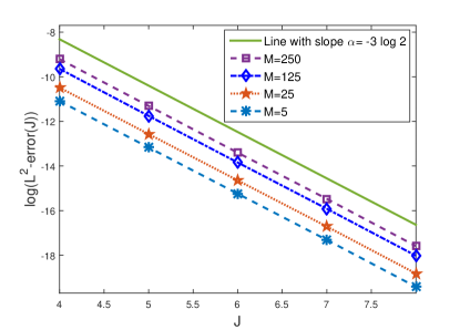
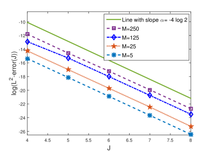
In the first example, the pricing of knock-out call discrete double barrier option is considered with the following parameters: $r=0.05$, $\sigma=0.25$, $T=0.5$, $S_{0}=100$, $E=100$, $U=120$ and $L=80~{},90~{},95~{},99~{},99.5$. In table 1, numerical results of presented method with Milev numerical algorithm [14], Crank-Nicholson [35], trinomial, adaptive mesh model (AMM) and quadrature method QUAD-K200 as benchmark [36] are compared for various number of monitoring dates. In addition, it can be seen that CPU time of presented method is fixed against increases of monitoring dates. The $L^{2}-error(J)$ are demonstrated for $L=90$ and $M=250$ in Table 2 which results verify the convergence rate of our algorithm. Fig.1 shows the plot of $log(L^{2}-error(J))$ for $r=3,4$ and it can be seen that the slope of $log(L^{2}-error(J))$ is near to $\alpha=-rlog(2)$.

(a) $r=3$

(b) $r=4$

Figure 1: $log(L^{2}-error(J))$ for example 1 with L=95

Table 1: Double barrier option pricing of Example 1: $T=0.5$, $r=0.05$, $\sigma=0.25$, $S_{0}=100$, $E=100$.

M	L	Presented Method (r=4 , J=5)	Milev ($200$)	Milev ($400$)	Trinomial	AMM-8	Benchmark
	80	2.4499	-	-	2.4439	2.4499	2.4499
	90	2.2028	-	-	2.2717	2.2027	2.2028
5	95	1.6831	1.6831	1.6831	1.6926	1.6830	1.6831
	99	1.0811	1.0811	1.0811	0.3153	1.0811	1.0811
	99.9	0.9432	0.9432	0.9432	-	0.9433	0.9432
CPU		0.25 s	1 s	5 s
	80	1.9420	-	-	1.9490	1.9419	1.9420
	90	1.5354	-	-	1.5630	1.5353	1.5354
25	95	0.8668	0.8668	0.8668	0.8823	0.8668	0.8668
	99	0.2931	0.2931	0.2931	0.3153	0.2932	0.2931
	99.9	0.2023	0.2023	0.2023	-	0.2024	0.2023
CPU		0.25 s	8 s	30 s
	80	1.6808	-	-	1.7477	1.6807	1.6808
	90	1.2029	-	-	1.2370	1.2028	1.2029
125	95	0.5532	0.5528	0.5531	0.5699	0.5531	0.5532
	99	0.1042	0.1042	0.1042	0.1201	0.1043	0.1042
	99.9	0.0513	0.0513	0.0513	-	0.0513	0.0513
CPU		0.25 s	35 s	150 s
	80	1.6165	-	-	1.8631	1.6163	1.6165
	90	1.1237	-	-	1.2334	1.1236	1.1237
250	95	0.4867	-	-	0.5148	0.4867	0.4867
	99	0.0758	-	-	0.0772	0.0759	0.0758
	99.9	0.0311	-	-	-	0.0311	0.0311
CPU		0.25 s

Table 2: $L^{2}-error$ of example 1 for $L=90$ and $M=250$.

	r=3		r=4
J	$e_{2}(J)$	${e_{2}(J-1)}/{e_{2}(J)}$	$e_{2}(J)$	${e_{2}(J-1)}/{e_{2}(J)}$
4	1.00241 e-4	-	7.45781 e -6	-
5	1.22740 e-5	8.16	4.65569 e-7	16.01
6	1.50805 e-6	8.14	3.31567 e-8	14.04
7	1.90330 e-7	7.92	2.18567 e-9	15.16
8	2.29513 e-8	8.29	1.40662 e-10	15.53

Example 2.

In this example, the parameters of knock-out call discrete double barrier option is considered as $r=0.05$, $\sigma=0.25$, $T=0.5$, $E=100$, $U=110$ and $L=95$. In table 3 the option price for different spot prices are evaluated and compared with Milev numerical algorithm [14], Crank-Nicholson [35] and the Monte Carlo (MC) method with $10^{7}$ paths [37].

Table 3: Double barrier option pricing of Example 2: $T=0.5$, $M=5$, $r=0.05$, $\sigma=0.25$, $E=100$, $U=110$ and $L=95$.

$S_{0}$	Presented Method (r=4 , J=5)	Crank-Nicolson (1000)	Milev (1000)	Milev (400)	MC (st.error) with $10^{7}$ paths
95	0.174498	0.1656	0.174503	0.174498	-
95.0001	0.174499	$\simeq$ 0.1656	0.174501	0.174499	0.17486 (0.00064)
95.5	0.182428	0.1732	0.182429	0.182428	0.18291 (0.00066)
99.5	0.229349	0.2181	0.229356	0.229349	0.22923 (0.00073)
100	0.232508	0.2212	0.232514	0.232508	0.23263 (0.00036)
100.5	0.234972	0.2236	0.234978	0.234972	0.23410 (0.00073)
109.5	0.174462	0.1658	0.174463	0.174462	0.17426 (0.00063)
109.9999	0.167394	$\simeq$ 0.1591	0.167399	0.167394	0.16732 (0.00062)
110	0.167393	0.1591	0.167398	0.167393	-
CPU	0.25 s	Minutes	1 s	39 s

Example 3.

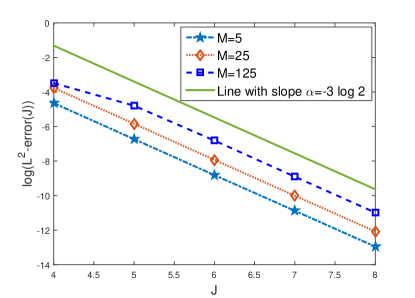
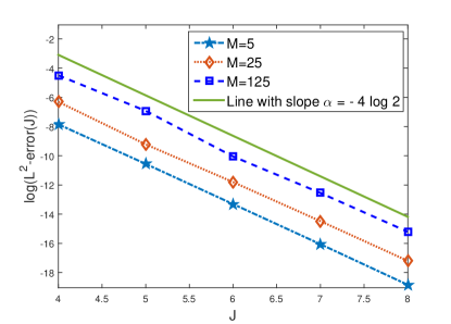
Due to the fact that the probability of crossing upper barrier during option’s life when $U\geq 2E$ is too small, the price of discrete single down-and-out call option can be estimated by double ones by setting upper barrier greater than $2E$ (for more details see[14]). Now, we consider a discrete single down-and-out call option with the following parameters: $r=0.1$, $\sigma=0.2$, $T=0.5$, $S_{0}=100$, $E=100$ and $L=95~{},99.5~{},99.9~{}$. The price is estimated by double ones with $U=2.5E$. The numerical results are shown in table 4 and compared with Fusaifls analytical formula [15], the Markov chain method (MCh)[38] and the Monte Carlo method (MC) with $10^{8}$ paths [11] that shows the validity of presented method in this case. Fig.2 shows the plot of $log(L^{2}-error(J))$ for $r=3,4$ and it can be seen that the slope of $log(L^{2}-error(J))$ is near to $\alpha=-rlog(2)$.

Table 4: Single barrier option pricing of Example 3: $T=0.5$, $r=0.1$, $\sigma=0.2$, $S_{0}=100$, $E=100$, $U=250$.

L	M	Presented Method (r=4 ,J=6)	Presented Method (r=4 ,J=7)	Fusai Analytical Method (IR17)	MCh	MC (st.error) with $10^{8}$ paths
95	25	6.63155	6.63156	6.63156	6.6307	6.63204 (0.0009)
99.5	25	3.35559	3.35558	3.35558	3.3552	3.35584 (0.00068)
99.9	25	3.00887	3.00887	3.00887	3.0095	3.00918 (0.00064)
95	125	6.16864	6.16864	6.16864	6.1678	6.16879 (0.00088)
99.5	125	1.96132	1.96130	1.96130	1.9617	1.96142 (0.00053)
99.9	125	1.51019	1.51021	1.51068	1.5138	1.5105 (0.00046)
CPU		0.48 s	0.83 s

(a) $r=3$

(b) $r=4$

Figure 2: $log(L^{2}-error(J))$ for example 3 with L=95

6 Conclusion and remarks

In this article, we used the Legendre multiwavelet for pricing discrete single and double barrier options. In section 4 we obtained a matrix relation 42 for solving this problem. Numerical results confirm that growth of computational time is negligible when the number of monitoring dates increase. On the other hand, the rate of convergence of presented algorithm has been obtained theoretically and verified numerically .

References

• [1] B. Kamrad, P. Ritchken, Multinomial approximating models for options with k state variables, Management science 37 (12) (1991) 1640–1652.
• [2] P. P. Boyle, S. H. Lau, Bumping up against the barrier with the binomial method, The Journal of Derivatives 1 (4) (1994) 6–14.
• [3] Y. K. Kwok, Mathematical models of financial derivatives. 1998.
• [4] R. C. Heynen, H. M. Kat, Barrier options, Exotic options: the State of the Art (1997) 125–159.
• [5] Y. S. Tian, Pricing complex barrier options under general diffusion processes, The Journal of Derivatives 7 (2) (1999) 11–30.
• [6] T.-S. Dai, Y.-D. Lyuu, The bino-trinomial tree: A simple model for efficient and accurate option pricing, The Journal of Derivatives 17 (4) (2010) 7–24.
• [7] D.-H. Ahn, S. Figlewski, B. Gao, Pricing discrete barrier options with an adaptive mesh model, Available at SSRN 162450.
• [8] L. Andersen, R. Brotherton-Ratcliffe, Exact exotics, Risk 9 (10) (1996) 85–89.
• [9] D. R. Beaglehole, P. H. Dybvig, G. Zhou, Going to extremes: Correcting simulation bias in exotic option valuation, Financial Analysts Journal (1997) 62–68.
• [10] P. Baldi, L. Caramellino, M. G. Iovino, Pricing general barrier options: a numerical approach using sharp large deviations, Mathematical Finance 9 (4) (1999) 293–321.
• [11] M. Bertoldi, M. Bianchetti, Monte carlo simulation of discrete barrier options, Financial engineering-Derivatives Modelling, Caboto SIM Spa, Banca Intesa Group, Milan, Italy 25 (2003) 1.
• [12] G. C. Kuan, N. Webber, Pricing barrier options with one-factor interest rate models, The Journal of Derivatives 10 (4) (2003) 33–50.
• [13] A. D. Andricopoulos, M. Widdicks, P. W. Duck, D. P. Newton, Universal option valuation using quadrature methods, Journal of Financial Economics 67 (3) (2003) 447–471.
• [14] M. Milev, A. Tagliani, Numerical valuation of discrete double barrier options, Journal of Computational and Applied Mathematics 233 (10) (2010) 2468–2480.
• [15] G. Fusai, I. D. Abrahams, C. Sgarra, An exact analytical solution for discrete barrier options, Finance and Stochastics 10 (1) (2006) 1–26. doi:10.1007/s00780-005-0170-y.
• [16] M. Broadie, Y. Yamamoto, A double-exponential fast gauss transform algorithm for pricing discrete path-dependent options, Operations Research 53 (5) (2005) 764–779.
• [17] F. Fang, C. W. Oosterlee, Pricing early-exercise and discrete barrier options by fourier-cosine series expansions, Numerische Mathematik 114 (1) (2009) 27.
• [18] A. Golbabai, L. Ballestra, D. Ahmadian, A highly accurate finite element method to price discrete double barrier options, Computational Economics 44 (2) (2014) 153–173.
• [19] M. Broadie, P. Glasserman, S. Kou, A continuity correction for discrete barrier options, Mathematical Finance 7 (4) (1997) 325–349.
• [20] G. Dorfleitner, P. Schneider, K. Hawlitschek, A. Buch, Pricing options with green’s functions when volatility, interest rate and barriers depend on time, Quantitative finance 8 (2) (2008) 119–133.
• [21] G. Fusai, M. C. Recchioni, Analysis of quadrature methods for pricing discrete barrier options, Journal of Economic Dynamics and Control 31 (3) (2007) 826–860.
• [22] C. Skaug, A. Naess, Fast and accurate pricing of discretely monitored barrier options by numerical path integration, Computational Economics 30 (2) (2007) 143–151.
• [23] M. A. Sullivan, Pricing discretely monitored barrier options, Journal of computational finance 3 (4) (2000) 35–52.
• [24] A. Pelsser, Pricing double barrier options using laplace transforms, Finance and Stochastics 4 (1) (2000) 95–104.
• [25] R. Farnoosh, H. Rezazadeh, A. Sobhani, M. H. Beheshti, A numerical method for discrete single barrier option pricing with time-dependent parameters, Computational Economics 48 (1) (2015) 131–145. doi:10.1007/s10614-015-9506-7.
• [26] R. Farnoosh, A. Sobhani, H. Rezazadeh, M. H. Beheshti, Numerical method for discrete double barrier option pricing with time-dependent parameters, Computers & Mathematics with Applications 70 (8) (2015) 2006–2013. doi:10.1016/j.camwa.2015.08.016.
• [27] R. Farnoosh, A. Sobhani, M. H. Beheshti, Efficient and fast numerical method for pricing discrete double barrier option by projection method, Computers & Mathematics with Applications.
• [28] T. Björk, Arbitrage theory in continuous time, Oxford university press, 2009.
• [29] W. A. Strauss, Partial differential equations, Vol. 92, Wiley New York, 1992.
• [30] B. K. Alpert, A class of bases in l^2 for the sparse representation of integral operators, SIAM journal on Mathematical Analysis 24 (1) (1993) 246–262.
• [31] M. Lakestani, B. N. Saray, M. Dehghan, Numerical solution for the weakly singular fredholm integro-differential equations using legendre multiwavelets, Journal of Computational and Applied Mathematics 235 (11) (2011) 3291–3303.
• [32] K. Atkinson, W. Han, Theoretical numerical analysis, Vol. 39, Springer.
• [33] M. A. Krasnosel’skii, P. P. Zabreiko, Geometrical methods of nonlinear analysis, 1984.
• [34] P. Anselone, T. Palmer, Spectral analysis of collectively compact, strongly convergent operator sequences, Pacific Journal of Mathematics 25 (3) (1968) 423–431.
• [35] B. Wade, A. Khaliq, M. Yousuf, J. Vigo-Aguiar, R. Deininger, On smoothing of the crank–nicolson scheme and higher order schemes for pricing barrier options, Journal of Computational and Applied Mathematics 204 (1) (2007) 144–158.
• [36] C.-J. Shea, Numerical valuation of discrete barrier options with the adaptive mesh model and other competing techniques, Master’s Thesis, Department of Computer Science and Information Engineering, National Taiwan University.
• [37] P. Brandimarte, Numerical methods in finance: a MATLAB-based introduction, Vol. 489, John Wiley & Sons, 2003.
• [38] J.-C. Duan, E. Dudley, G. Gauthier, J.-G. Simonato, Pricing discretely monitored barrier options by a markov chain, The Journal of Derivatives 10 (4) (2003) 9–31.