Immersed transient eddy current flow metering: a calibration-free velocity measurement technique for liquid metals

Abstract

Eddy current flow meters (ECFM) are widely used for measuring the flow velocity of electrically conducting fluids. Since the flow induced perturbations of a magnetic field depend both on the geometry and the conductivity of the fluid, extensive calibration is needed to get accurate results. Transient eddy current flow metering (TECFM) has been developed to overcome this problem. It relies on tracking the position of an impressed eddy current system which is moving with the same velocity as the conductive fluid. We present an immersed version of this measurement technique and demonstrate its viability by numerical simulations and a first experimental validation.

Keywords: flow measurement, inductive methods, calibration-free

1 Introduction

Measuring the flow velocity of liquid metals is a challenging task because of their opacity, chemical reactivity and - in most cases - elevated ambient temperature [1]. Fortunately, the high electrical conductivity of liquid metals often allows to use magnetic inductive measurement techniques. These techniques generally rely on applying magnetic fields to the fluid and measuring appropriate features, e.g. amplitudes, phases, or forces, of the flow induced magnetic fields.

A local embodiment of this technique is the eddy current flow meter (ECFM) as patented by Lehde and Lang in 1948 [2], which consists of two primary coils excited by an AC generator, and one secondary coil located midway between them. Modifications of this method, using one primary coil and two secondary coils, were described in [3, 4]. Another version of this local sensor, which measures the flow induced change of the amplitude in the vicinity of a small permanent magnet, is the magnetic-distortion probe described by Miralles et al. [5].

A global embodiment of the same principle, the contactless inductive flow tomography (CIFT), is able to reconstruct entire two or three-dimensional flow fields from induced field amplitudes that are measured at many position around the fluid when it is exposed to one or a few external magnetic fields [6, 7, 8].

Another inductive measurement concept relies on the determination of magnetic phase shifts due to the flow [9, 10]. Further, the Lorentz force velocimetry (LFV) determines the force acting on a permanent magnet close to the flow, which results as a direct consequence of Newton’s third law applied to the braking force acting by the magnet on the flow [11]. With this technique, it is even possible to measure velocities of fluids with remarkably low conductivities, such as salt water [12].

A common drawback of (nearly) all those methods is that they require extensive calibration since the flow induced magnetic field perturbations depend both on geometric details of the measuring system and on the conductivity of the fluid, which is, in turn, temperature-dependent. Actually, the signals are proportional to the magnetic Reynolds number $Rm=\mu_{0}\sigma VL$, where $\mu_{0}$ is the magnetic permeability constant, $\sigma$ the conductivity of the liquid, and $V$ and $L$ denote typical velocity and length scales of the relevant fluid volume. Further to this, the use of permanent magnets, as necessary for the magnetic distortion probe [5] and for LFV [11], or of magnetic yoke materials, as for the phase-shift method [9, 10], set serious limitations to the ambient temperature at the position of the respective sensors.

Transient eddy current flow metering (TECFM) [13] aims at overcoming both drawbacks. Building upon earlier work of Zheigur and Sermons [14], this is accomplished by impressing a traceable eddy current system into the liquid metal and detecting its movement with appropriately positioned magnetic field sensors. Since the eddy current moves with the velocity of the liquid, there is no need for a calibration of the sensor. The non-invasive TECFM sensor for measuring the liquid metal velocity close to the fluid boundary from outside, as described in [13], represents a specific external realization of TECFM.

Here, we present a modified variant of TECFM, an invasive sensor that can be placed within a liquid metal pool or a pipe to measure the local velocity in the surrounding metal. After describing the main functioning principle of this immersed transient eddy current flow metering (ITECFM), we will illustrate the method by numerical simulations. Then, first flow measurements in the eutectic alloy GaInSn will be presented. The paper closes with some conclusions and a discussion of the prospects to use the method under high temperature conditions.

2 The principle of ITECFM

ITECFM is intended to measure the local velocity or the flow rate around the sensor in liquid metal pools or large pipes (for small pipes there will be some distortion of the results, when the penetration depth of the magnetic field into the liquid metal is larger than the radius of the pipe). Basically, the ITECFM sensor is an invasive tube-shape sensor which is put inside the liquid metal, parallel to the flow direction. There is no direct contact between the liquid metal and the pick-up coils because the latter are protected by a cladding, made of stainless steel for example. In contrast to the external variant of TECFM [13], this configuration traces the zero crossing of the magnetic field of the eddy current system instead of the position of a magnetic pole. For this purpose, the coils are arranged differently in order to allow a velocity measurement of the surrounding liquid.

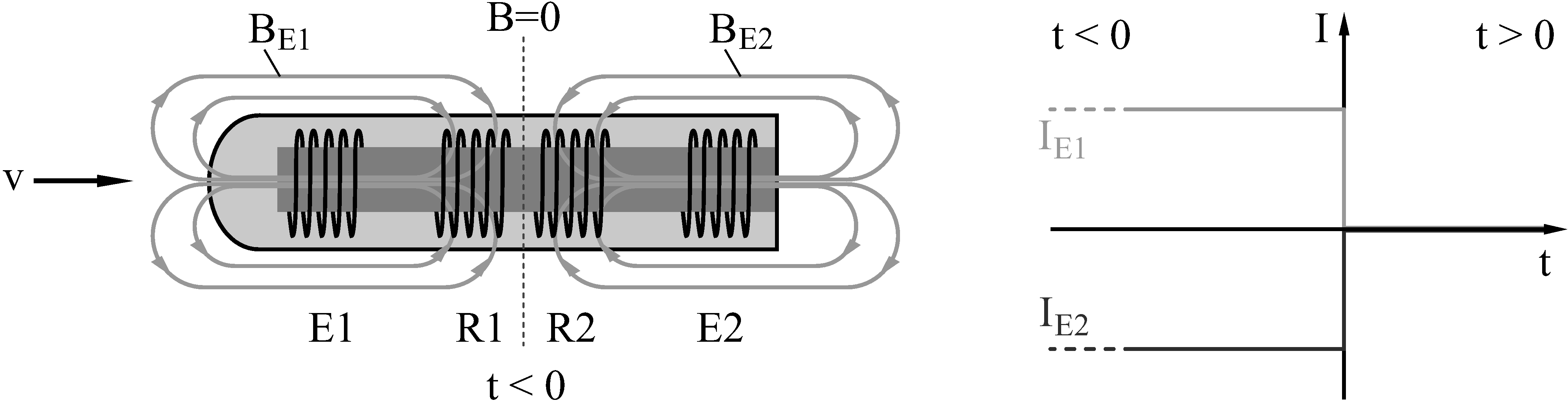
Figure 1: Basic structure of the ITECFM sensor and its magnetic field produced by the two excitation coils E1, E2 before the excitation currents are switched off. The induced voltages are measured by the two receiver coils R1 and R2. The time dependent excitation currents $I_{\mathrm{E1}}$ and $I_{\mathrm{E2}}$ are displayed on the right hand side.

The eddy currents within the liquid metal, which are to be used for inferring the fluid velocity, are induced by the excitation coils E1 and E2 (see figure 1). Figure 2 shows a simplified scheme of these eddy currents. Both magnetic fields $B_{\mathrm{E1}}$ and $B_{\mathrm{E2}}$ are generated by current steps which occur at the same time, but in opposite directions. The result are two oppositely directed magnetic fields with the same amplitude, which will induce opposing eddy currents during switching on or off of the excitation currents. Because of the symmetric arrangement of the coils (and, therefore, the magnetic fields), the zero crossing $x_{\mathrm{0}}$ of the total magnetic field $B$ is located exactly in the middle between the receiver coils R1 and R2, when $v_{\mathrm{liquid}}$ is zero and/or immediately after the current step for $v_{\mathrm{liquid}}>0$. The excitation currents are assumed to be switched off at $t=0$.

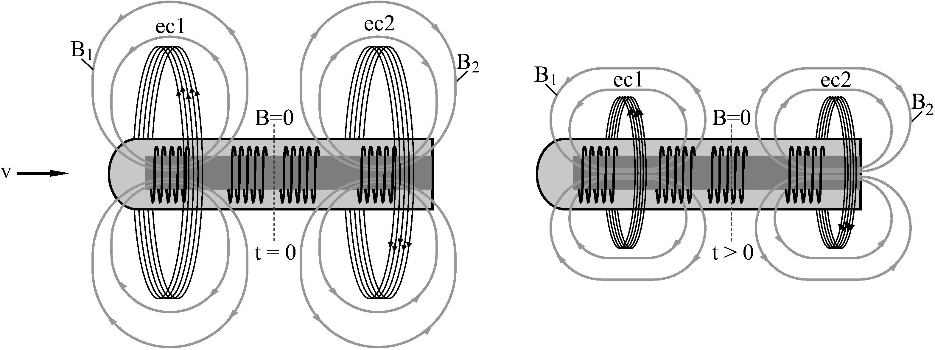
Figure 2: Immersed TEC-FM: Eddy currents ec1 and ec2 induced within the liquid metal and their magnetic fields $B_{\mathrm{1}}$, $B_{\mathrm{2}}$ when the excitation currents are switched off at $t=0$ (left) and for $t>0$ (right) when the eddy currents have started to move in flow direction and begin to dissipate.

Although the eddy currents ec1, ec2 and their magnetic fields $B_{\mathrm{1}}$, $B_{\mathrm{2}}$ are dissipating [15], for $v_{\mathrm{liquid}}=0$ the zero crossing remains exactly in their middle, regardless of their magnitude. This changes, however, if the fluid is moving. Then, the eddy currents are transported in flow direction with the velocity of the fluid. Under the reasonable assumption that the electrical conductivity of the liquid metal is homogeneous around the sensor, both eddy currents will dissipate with the same rate and the zero crossing of the magnetic field will also move with the fluid velocity. The position of the zero crossing can be tracked by means of the receiver coils R1 and R2.

Just as in [13], the position of the zero crossing can be calculated according to

$$x_{0}(t) = \frac{x_{1}\dot{B}_{\mathrm{2}}(t)-x_{2}\dot{B}_{\mathrm{1}}(t)}{\dot{B}_{\mathrm{2}}(t)-\dot{B}_{\mathrm{1}}(t)}=\frac{x_{1}U_{2}(t)-x_{2}U_{1}(t)}{U_{2}(t)-U_{1}(t)}$$ (1)

where $x_{1}$ and $x_{2}$ are the positions of the receiver coils R1 and R2, and $U_{1}$ and $U_{2}$ are the respective voltages measured there. Although the arrangement of the coils for the external TECFM is different, this simplified formula can be used to approximate the liquid metal velocity in the case of ITECFM, too. This will be validated by numerical simulations in the next section.

3 Numerical simulations

The simulations of ITECFM were implemented in COMSOL Multiphysics 5.0, using a time dependent 2D axisymmetric model and the magnetic fields (mf) physics environment.

3.1 Simulation Model

For the simulation, some simplifications have been made. The flow velocity $v_{\mathrm{liquid}}$ of the liquid metal is assumed constant and homogeneous around the sensor thimble. The liquid metal does not contain foreign particles or gas bubbles. Furthermore, any Lorentz forces exerted by the excitation coils on the liquid metal are neglected.

For an optimal operation of the sensor, the receiver coils should be arranged symmetrically, with the centre of symmetry exactly in the middle between the two excitation coils (see dashed horizontal line in figure 3). Reasonable positions of the receiver and excitation coils have been determined by multiple simulations with variations in arrangement, size and spacing between the coils. In principle, there are two possibilities for the arrangement of the coils: the receiver coils can be placed between the excitation coils or vice versa. However, since the initial position $x_{\mathrm{0}}$ of the zero crossing of the magnetic field is located exactly in the middle between the excitation coils, the receiver coils should be placed as close as possible to this point in order to achieve maximum sensitivity of the sensor. Placing the excitation coils between the receiver coils is also possible but would result in a much lower signal amplitude and sensitivity because of the increased distance from $x_{\mathrm{0}}$.

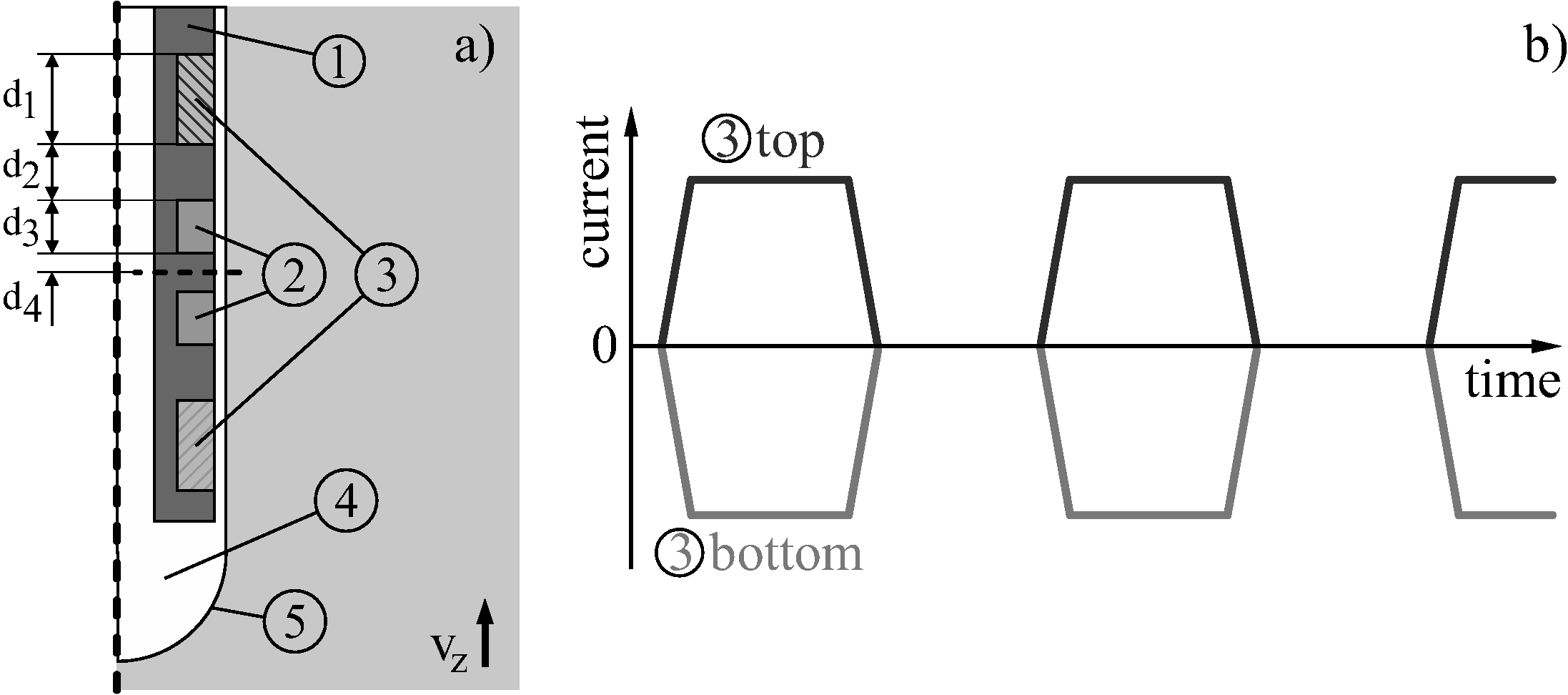
Figure 3: a) Simplified simulation model of the ITECFM sensor: 1 - coil holder (core), 2 - receiver coils, 3 - excitation coils, 4 - air, 5 - sensor thimble, $v_{z}$ indicates the flow direction of the liquid metal, the dashed vertical line represents the symmetry axis for the 2D axisymmetric model, the dashed horizontal line shows the position of the centre of symmetry regarding the coils ($d_{\mathrm{1}}=5$ mm, $d_{\mathrm{2}}=3$ mm, $d_{\mathrm{3}}=3$  mm, $d_{\mathrm{4}}=1$ mm). b) Excitation current pulses for the top and bottom excitation coil

The size of the excitation coils turn out to have only a minor influence on the functionality of the sensor, as long as the absolute values of the excitation current pulses are the same, since $x_{\mathrm{0}}$ is always in the middle between them. Their actual size was chosen to accommodate a reasonable number of turns for the coil wires in the actual prototype. However, the axial extension of the receiver coils should be as small as possible because this will increase their sensitivity for detecting the zero crossing of the magnetic field, and also minimize the dependence on the conductivity of the liquid. Further to this, since the distance between the coils and the boundary of the liquid metal has a significant influence on the signal strength, the air gap between coils and inner wall of the sensor, as well as the wall thickness of the sensor thimble, should be as small as possible. The actual sizes, turn numbers, and wire thicknesses of the coils for a low temperature (LT) and a high temperature (HT) prototype of the ITECFM sensor are shown in table 1 (see also figure 3 a). A photography of the high temperature sensor is shown in figure 4.

Table 1: Properties of the low temperature(LT) and high temperature(HT) prototypes

	LT Sensor	HT Sensor
Receiver coils: height	3 mm	5 mm
Excitation coils: height	5 mm	8 mm
Receiver coils: turns	120	80
Excitation coils: turns	100	120
Receiver coils: wire thickness	0.15 mm	0.25 mm
Excitation coils: wire thickness	0.25 mm	0.25 mm
Max. operation temperature	$150^{\circ}$ C	$650~{}^{\circ}C$
Core material	PVC	ceramic
Wire material	copper	73% copper, 27% nickel
Wire isolation	enamel	ceramic

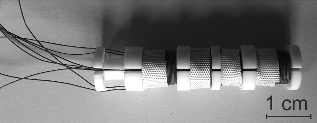
Figure 4: High temperature prototype of the ITECFM sensor for temperatures up to 650 ^∘C.

3.2 Simulation results

The edge steepness of the excitation current plays an important role for ITECFM because the fluid velocity can only be extracted from the magnetic fields when the excitation currents have reached their final value, i.e. $dI/dt=0$. From this instant on, R1 and R2 detect exclusively the magnetic fields of the eddy currents within the liquid.

In figure 5 we see how the time derivatives of the fields $B_{1}$ and $B_{2}$ at the two receiver coils R1 and R2 change with increasing fluid velocity. For this example, the three top curves show the values for $\dot{B}_{1}$ and the three bottom curves the values for $\dot{B}_{2}$. While they are symmetrical for $v_{\mathrm{liquid}}=0$, there is a growing asymmetry between $\dot{B}_{1}$ and $\dot{B}_{2}$ for increasing $v_{\mathrm{liquid}}$.

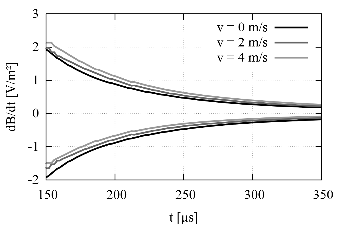
Figure 5: Simulation results of $\dot{B}_{\mathrm{1}}$ and $\dot{B}_{\mathrm{2}}$ as a function of time, computed for three fluid velocities $v_{\mathrm{liquid}}$ and the conductivity of GaInSn $\sigma=3.3\times 10^{6}$ S/m. The excitation current is supposed to be switched off at $t=0~{}\mu$ s and to reach zero at $t=100~{}\mu$ s.

When plotting $\dot{B}$ on a line parallel to the flow direction at different instants in time after the current steps, the movement of the zero crossing can clearly be seen (figure 6). Although the magnetic field is significantly dissipating with time, the zero crossing of $\dot{B}$ keeps moving with $v_{\mathrm{liquid}}$. This is shown in the right panel of figure 6 , where $x_{0}$ marks the time-dependent position of the zero crossing.

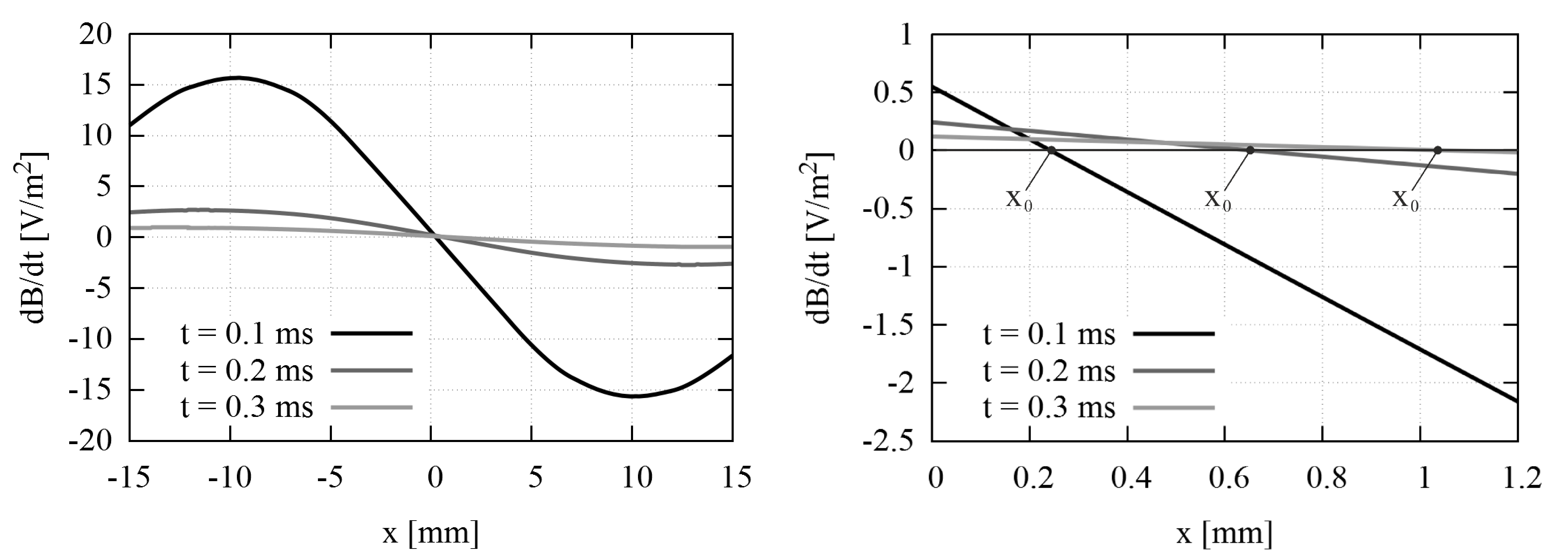
Figure 6: Simulation results of the time derivative of the total magnetic field for $v_{\mathrm{liquid}}=4$ m/s in a range of $\pm 15$ mm around the centre of the sensor (left), and a zoom to $x=0$ mm (right) after 0.1 ms, 0.2 ms and 0.3 ms. $x=0$ mm is located exactly in the middle between the coils R1 and R2. $x_{\mathrm{0}}$ shows the time-dependent position of the zero crossing of $\dot{B}$.

Figure 7 shows the movement of $x_{\mathrm{0}}$ over time. The fluid velocity is then inferred from the slope of the respective line in the data set. Since, in this particular simulation, the excitation currents reach zero only at $100~{}\mu$ s, before that instant $x_{\mathrm{0}}(t)$ appears to move slower than the fluid velocity.

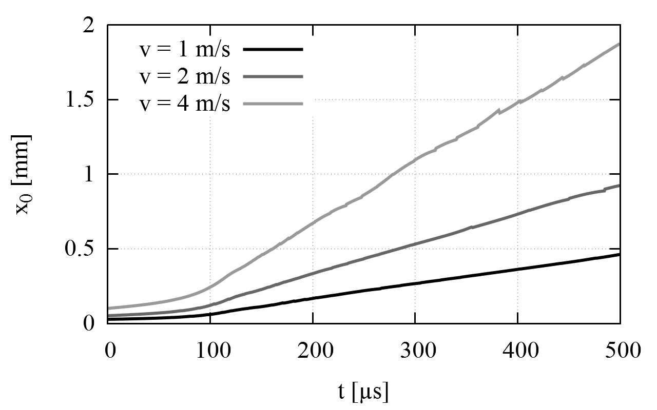
Figure 7: Simulation results for the time dependent position $x_{\mathrm{0}}(t)$ for three different velocities. The current steps reach their final value after $100~{}\mu$s.

The reason for this effect is the superimposition with the remaining magnetic fields of the excitation coils. For laboratory experiments it is therefore advisable to use a current source with a high edge steepness. Otherwise $B_{1}$ and $B_{2}$ would have already dissipated too much for an accurate measurement.

While we have considered the case of switching off the excitation current, almost the same results are obtained for switching on the currents. Although the magnetic fields of the excitation coils are not zero, they are constant after they reach their final value and would not induce currents within the excitation coils or the liquid metal. Yet, the difference between both methods would become larger for increasing $Rm$.

Until now, the simulations have been calculated only for one electrical conductivity of the liquid metal ($\sigma=3.3\times 10^{6}$ S/m for GaInSn). With view on the strong influence of the (temperature dependent) conductivity for conventional ECFM’s, we present in figure 8 the calculated velocity for different conductivities and a variety of hypothetical (and real) coil geometries.

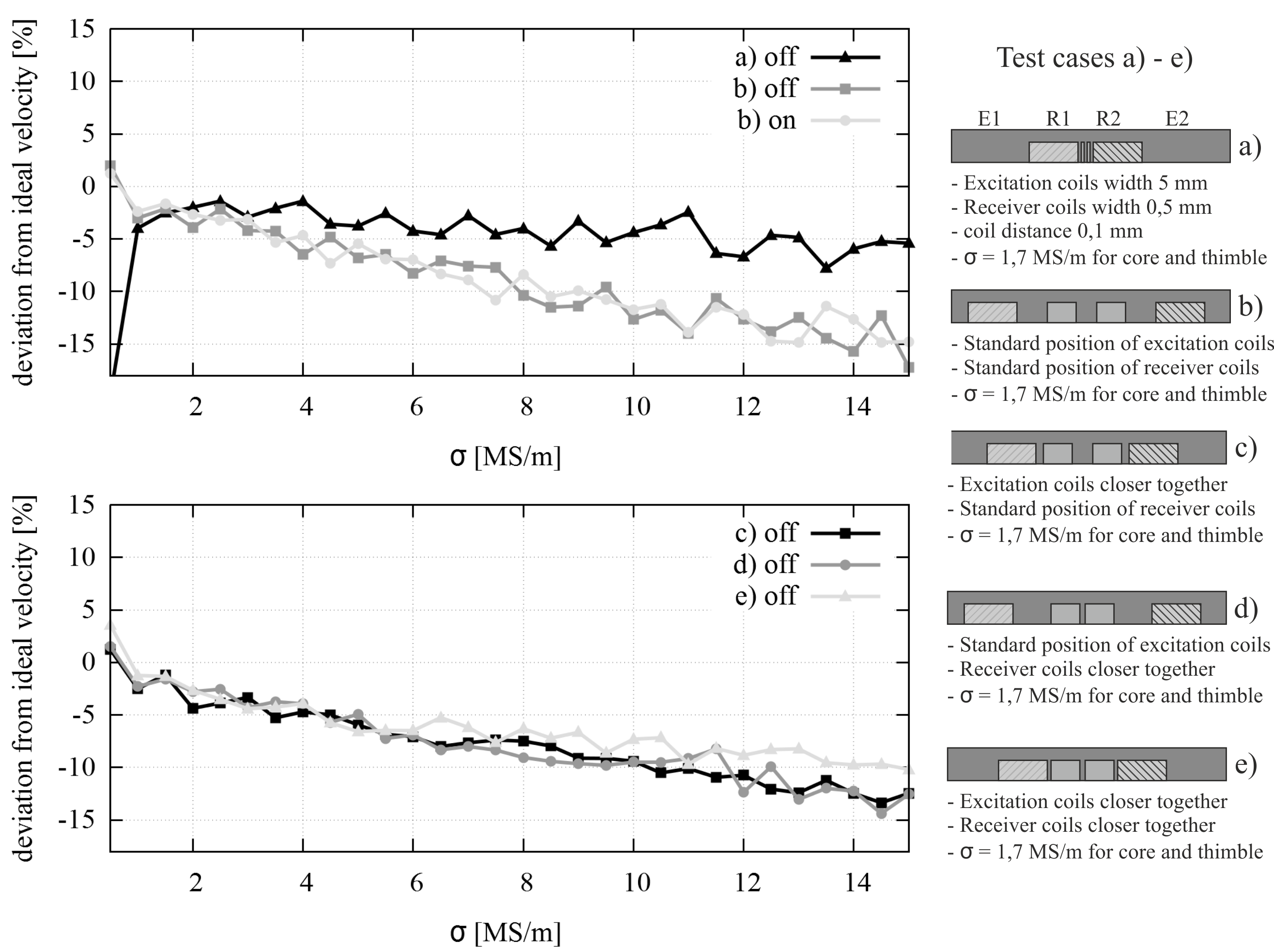
Figure 8: Simulation results for the deviation of the measured velocity from the pre-given velocity for different coil geometries and varying electrical conductivity of the liquid metal for $v_{\mathrm{liquid}}=2$ m/s when switching off (on) the excitation current.

In general, despite some slight dependence on the electrical conductivity of the fluid, the deviation from the ideal velocity is relatively weak for a wide range of conductivities. Hence, ITECFM can essentially be considered as calibration-free. In the case of extremely thin receiver coils (a), the overall deviation would remain less than 5% for $1$ MS/m $<\sigma<10$ MS/m. For the standard geometry (as embodied in the prototypes for which the coil size and distance between the coils have to be larger in order to accommodate a suitable number of turns and to facilitate the construction of the core) it can be seen (b and c) that the results for switching on or switching off the excitation currents are almost the same. The further simulation (c,d,e) show also that the deviation from the ideal velocity is smaller, when the coils are positioned as close to each other as possible, especially at high conductivities. At low conductivities of the liquid metal, the positioning of the coils has only a small influence on the results. The increasing deviations for higher fluid conductivities are related to the size of and the distance between the coils as well as the dissipation of the eddy currents.

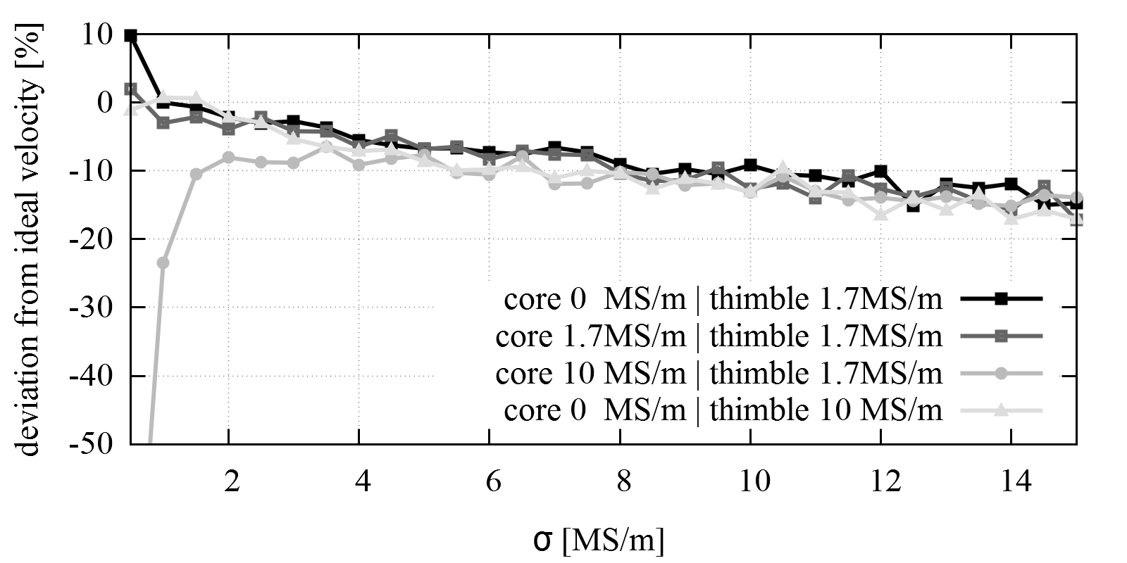
Figure 9: Simulation results for the deviation of the measured velocity from the pre-given velocity for different electrical conductivities of sensor core and thimble and varying electrical conductivity of the liquid metal for $v_{\mathrm{liquid}}=2$ m/s when switching off the excitation current. The coils are arranged like in the standard case b).

As can be seen in figure 9, the electrical conductivity of the sensor core, which holds the coils, and of the sensor thimble have a significant influence on the measurement results for the velocity, especially at low $\sigma$ of the liquid metal. The eddy currents which are induced within the conductive components of the sensor, are stronger for higher electrical conductivities. Unlike the eddy currents within the liquid metal, they are not moving with $v_{\mathrm{liquid}}$ but are stationary at all times. Because the magnetic fields of the eddy currents from liquid metal are superimposed with the fields of the sensor components, the measured velocity appears to be lower. This effect is stronger at low $\sigma$ of the liquid metal because the eddy currents within the sensor components are in the same order of magnitude or even larger than the ones in the liquid metal. Another aspect to consider is the volume of the respective sensor components. Because the core has a considerable larger volume than the thimble wall, its conductivity has a larger influence on the velocity measurement. At higher $\sigma$ of the liquid metal the effect gets more and more negligible because of the stronger eddy currents and the larger volume of the liquid metal.

4 Experimental results

A first test of a ITECFM sensor was carried out with the low-temperature prototype in a liquid metal loop with the eutectic alloy GaInSn. This sensor has a plastic coil holder, the excitation coils have 100 turns, the receiver coils have 120 turns, and conventional copper wire of diameter 0.25 mm was used (see table 1). Rectangular voltage pulses of $5~{}V$ with a frequency of 1 kHz, a duty cycle of 50 % and a fall time of $20~{}\mu$s have been used to generate the excitation currents.

The sensor was put inside a stainless steel tube to prevent direct contact with the liquid metal. The receiver voltages were measured with a memory oscilloscope and $x_{\mathrm{0}}(t)$ was calculated with equation (1). Figure 10 shows the measurement results for four different fluid velocities and a linear fit of each dataset. The displayed results represent the mean value of 2500 measurement sweeps with one measurement taken every millisecond for $2.5s$. As can be seen in the previous section in figure 7, the results for $x_{\mathrm{0}}(t)$ are expected to have a linear rise.

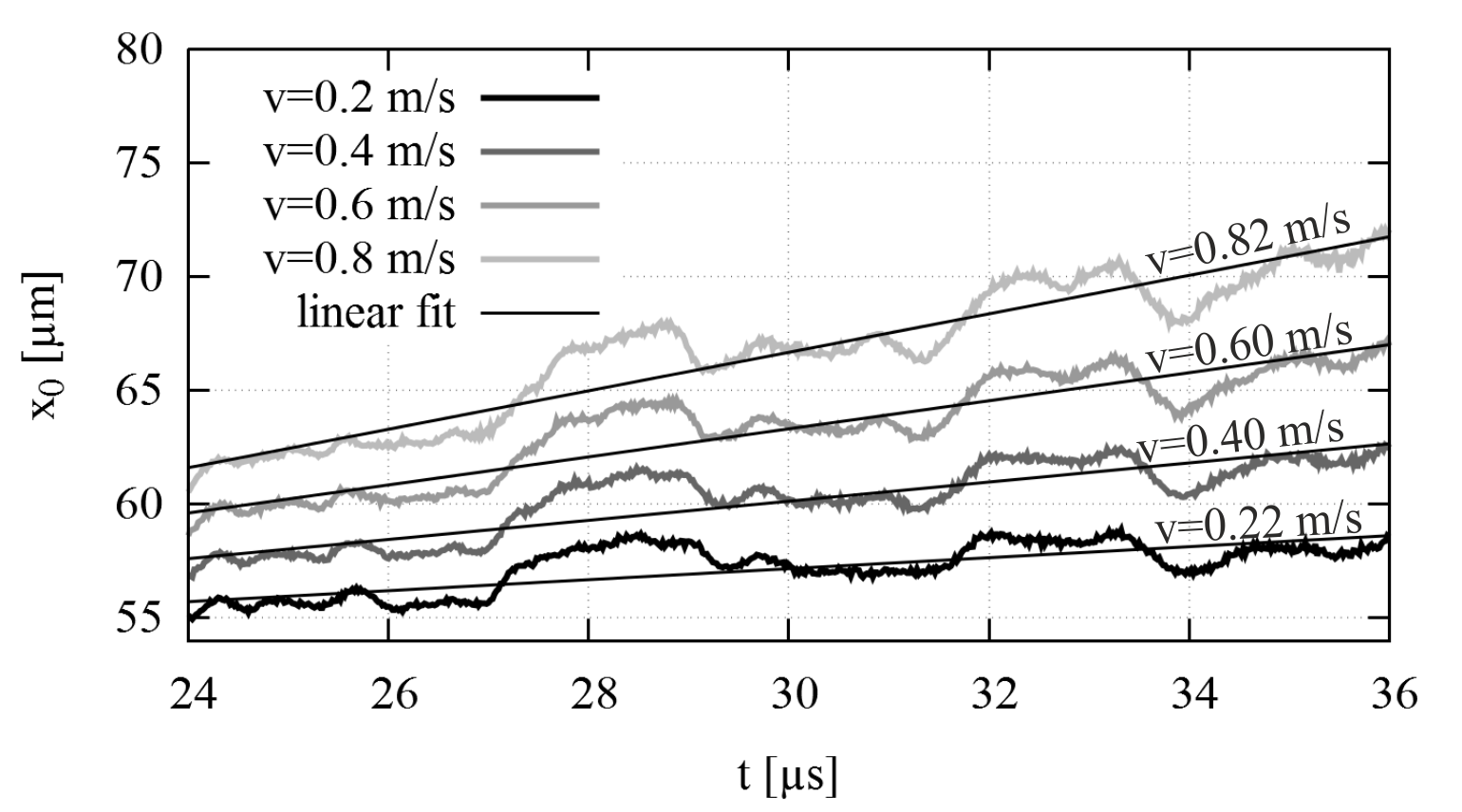
Figure 10: Measurement results for the movement of $x_{\mathrm{0}}$ for ITECFM in a pipe flow of GaInSn. The fluid velocity is inferred from the slope of the respective linear fit for each pre-adjusted velocity. The inferred velocity is indicated above each curve.

There are some deviations from the expected results for $x_{\mathrm{0}}(t)$, especially the disturbances around $t=28~{}\mu$s and $t=33~{}\mu$s. The overall slope of the linear fit however, is very close to the pre-adjusted flow velocity in the GaInSn-Loop (which is, as a matter of fact, also not exactly known). The disturbances appear at the same times for each measurement and are most likely caused by the resonant frequency of the receiver coils. Future experiments using tailored current sources instead of the presently used voltage source are expected to improve this situation.

5 Conclusions and prospects

In this paper, we have presented the principle of ITECFM and some promising results obtained both in simulations as well as in an experiment with a first prototype in GaInSn. While its calibration-free character makes the method a promising candidate for a number of laboratory and industrial applications, it certainly needs further tests and optimization. Although both the external and immersed configurations of TECFM are based on the same principle, there are some differences with view on the different arrangement of the excitation and receiver coils, which have to be addressed in detail.

Future work will be devoted to more experiments with optimized excitation schemes and different liquid metals to validate the simulation results and the calibration free-free character of the sensor. Another advantage of ITECFM is the avoidance of any magnetic materials which makes it particularly suited for high temperature applications. Tests with the high temperature prototype consisting of heat resistant materials are planned for ambient temperatures of up to 650 ^∘C as they are typical, e.g., for sodium fast reactors.

References

References

- [1] Eckert S, Buchenau D, Gerbeth G, Stefani F and Weiss FP 2011 Some recent developments in the field of measuring techniques and instrumentation for liquid metal flows J. Nucl. Sci. Techn. 48 490-9
- [2] Lehde H, Lang WT 1948 Device for measuring rate of fluid flow US Patent 2435043
- [3] Sureshkumar S et al. 2013 Utilization of eddy current flow meter for sodium flow measurement in FBRs Nuclear Engineering and Design, 265 1223-31
- [4] Poornapushpakala S, Gomathy C, Sylvia JI, Babu B 2014 Design, development and performance testing of fast response electronics for eddy current flow meter in monitoring sodium flow Flow Meas. Instrum. 38 (2014)98-107
- [5] Miralles S, Verhille G, Plihon N, Pinton JF 2011 The magnetic-distortion probe: velocimetry in conducting fluids Rev. Sci. Instrum. 82 095112
- [6] Stefani F and Gerbeth G 2000 A contactless method for velocity reconstruction in electrically conducting fluids Meas. Sci. Techn. 11 758-65
- [7] Stefani F, Gundrum T and Gerbeth G 2004 Contactless inductive flow tomography Phys. Rev. E 70 056306
- [8] Wondrak T, Galindo V, Gerbeth G, Gundrum T, Stefani F and Timmel K 2010 Contactless inductive flow tomography for a model of continuous steel casting Meas. Sci. Techn. 21 045402
- [9] Priede J, Buchenau D and Gerbeth G 2011 Contactless electromagnetic phase-shift flowmeter for liquid metals Meas. Sci. Techn. 22 055402
- [10] Priede J, Buchenau D and Gerbeth G 2009 Force-free and contactless sensor for electromagnetic flowrate measurements Magnetohydrodynamics 45 451-8
- [11] Thess A, Votyakov E V and Kolesnikov Y 2006 Lorentz force velocimetry Phys. Rev. Lett. 96 164501
- [12] Halbedel B et al 2014 A novel contactless flow rate measurement device for weakly conducting fluids based on Lorentz force velocimetry Flow Turb. Comb. 92 361-9
- [13] Forbriger J and Stefani F 2015 Transient eddy current flow metering Meas. Sci. Techn. 26 105303
- [14] Zheigur BD and Sermons GY 1965 Pulse method of measuring the rate of flow of a conducting fluid Magnetohydrodynamics 1 (1) 101-104
- [15] Forbriger J, Galindo V, Gerbeth G and Stefani F 2008 Measurement of the spatio-temporal distribution of harmonic and transient eddy currents in a liquid metal Meas. Sci. Technol. 19 045704