Signatures of a $4\pi$-periodic supercurrent in the voltage response of capacitively shunted topological Josephson junctions

Abstract

We investigate theoretical aspects of the detection of Majorana bound states in Josephson junctions using a semiclassical model of the junction. The influence of a $4\pi$-periodic supercurrent contribution can be detected through its effect on the width of the Shapiro steps and the Fourier spectrum of the voltage. We explain how the inclusion of a capacitance term results in a strong quenching of the odd steps when the junction is underdamped, which may be used to effectively detect Majorana bound states. Furthermore, in presence of capacitance the first and third steps are quenched to a different degree, as observed experimentally. We examine the emission spectrum of phase-locked solutions, showing that the presence of period-doubling may complicate the measurement of the $4\pi$-periodic contribution from the Fourier spectrum. Finally, we study the voltage response in the quasiperiodic regime and indicate how the Fourier spectra and the first-return maps in this regime reflect the change of periodicity in the supercurrent.

I Introduction

Topological degenerated states in quantum systems are subject of present active research, both for their fascinating fundamental physical properties and for the possibility of using them as a platform for topological quantum computation (Tewari et al., 2007; Nayak et al., 2008; Bonderson and Lutchyn, 2011; Jiang et al., 2011). Topological phases of superconductors which support Majorana bound states(MBS) (Kitaev, 2001; Fu and Kane, 2008) can be implemented in solid state setups presenting spin-orbit coupling, broken time-reversal symmetry and superconductivity. Different experimental configurations to detect MBS have been proposed (Bolech and Demler, 2007; Benjamin and Pachos, 2010; Akhmerov et al., 2011; Beenakker, 2013). In particular, MBS can be detected in Josephson junctions (Tanaka et al., 2009; Pikulin and Nazarov, 2012; Tkachov and Hankiewicz, 2013), through either zero-bias conductance peaks (Mourik et al., 2012) or its effect on the current-phase relation in the dc Josephson effect (Olund and Zhao, 2012). Recently, the current-phase relation in a Josephson junction formed by one-dimensional nanowires featuring MBS has been observed experimentally through the vanishing of the odd Shapiro steps in ac biased Josephson junctions (Rokhinson et al., 2012; Wiedenmann et al., 2016; Bocquillon et al., 2016; Deacon et al., 2016), showing that this setup can be used to effectively detect MBS.

The appearance of Shapiro steps is one example of non-linear phenomena in mesoscopic systems  (Okuyama et al., 1981; He et al., 1985; Pedersen, 1993; Ambika, 1997). Non-linear transport in different solid state systems has been analyzed in the past (Shaw et al., 1992; Jalabert et al., 1994; Bulashenko and Bonilla, 1995; Bonilla and Grahn, 2005), showing interesting regimes, such as quasiperiodicity(Bohr et al., 1984; Jensen et al., 1984), frequency locking(Kautz, 1996; Waldram et al., 1970) and different routes to chaos (He et al., 1984; Gwinn and Westervelt, 1987; Luo et al., 1998a; Alhassid, 2000). In that direction, one promising area of research focuses on the relationship between topology and non-linearity. For example, the interplay between topology and instabilities has been recently analyzed in bosonic systems under ac driving (Engelhardt et al., 2016a) and junction arrays mimicking the SSH model (Engelhardt et al., 2016b). The Shapiro experiment in a topological Josephson junction has been theoretically analyzed by means of a semiclassical RSJ model (Domínguez et al., 2012; Sau and Setiawan, 2016; Domínguez et al., 2017), and with a finite capacitance in the high ac-bias limit (Maiti et al., 2015).

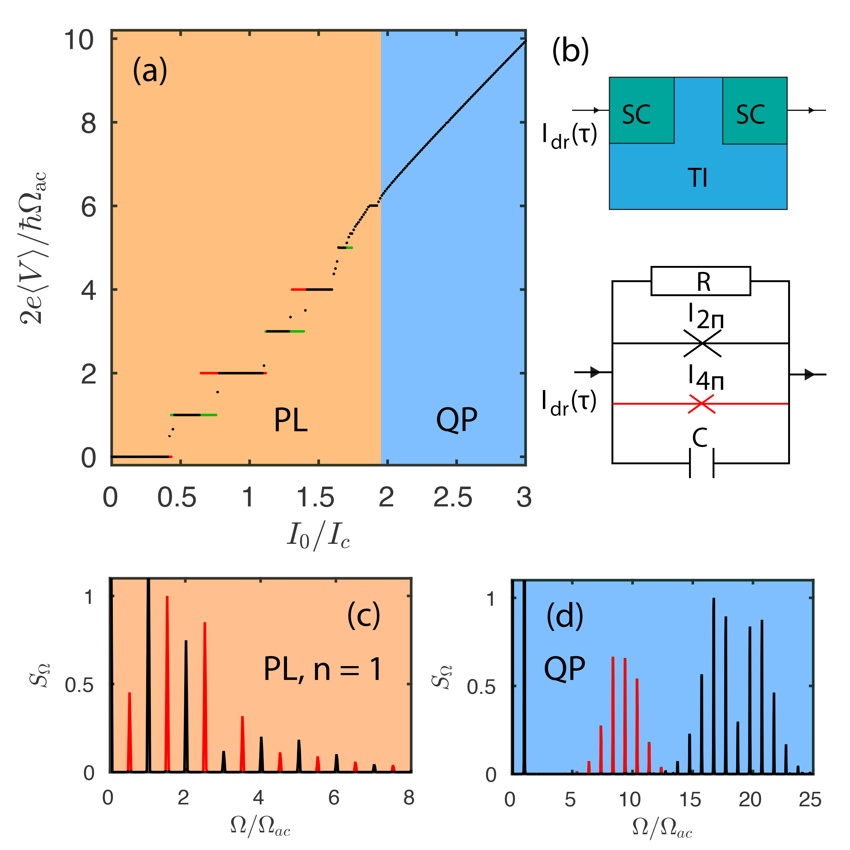
Figure 1: (a) $I_{0}-\mathcal{h}V\mathcal{i}$ curve showing Shapiro steps corresponding to the phase-locked regime (PL, orange) and a linear $I_{0}-\mathcal{h}V\mathcal{i}$ section for the quasiperiodic regime (QP, blue). The reduction (increase) in the odd (even) steps for $I_{4\pi}=0.3I_{2\pi}$ is marked in green (red). (b) Top: scheme of a topological Josephson junction. Superconductivity is induced into a topological insulator (TI, blue) through the proximity effect by a superconductor (SC, green). Bottom: circuit representation of the junction in the RCSJ model, with elements corresponding to the resistive (R), capacitive (C) and the ordinary ($I_{2\pi}$) and $4\pi$-periodic ($I_{4\pi}$) supercurrent channels. (c), (d) Fourier spectra from a PL solution in the first Shapiro step and from a QP solution, respectively. The peaks in red are a result of the $4\pi$-periodic supercurrent.

In this work we investigate both the phase-locked and the quasiperiodic regimes of a capacitively shunted Josephson Junction driven by an ac current in presence of a $4\pi$-periodic supercurrent contribution. This paper is organized as follows. In Sec. II we introduce the RCSJ model to describe such a system. In Sec. III we study the influence of a $4\pi$-periodic contribution on the width of the Shapiro steps and indicate the parameter regions where the junction is strongly affected by the change in the periodicity of the supercurrent. In Sec. IV we consider the possibility of measuring the emission spectrum of the junction from both the phase-locked and quasiperiodic regimes in order to detect MBS.

II Theoretical Model

The study of the current-driven Josephson junction is a difficult task from the microscopic point of view. It does not only involve out of equilibrium processes but also strong Coulomb interactions and dissipation. The problem becomes drastically simplified in the semiclassical limit, yielding the resistively capacitively shunted junction (RCSJ) model (McCumber, 1968), represented schematically in Fig. 1 (b). This model describes the evolution of the superconducting phase difference $\varphi$ by means of the equation of motion $CdV/dt+V/R+I_{\mathrm{sc}}(\varphi)=I_{\mathrm{dr}}(\tau)$, which results from equating the external current bias, which we take as $I_{\mathrm{dr}}(\tau)=I_{0}+I_{1}\mathrm{sin}(\Omega_{\mathrm{ac}}\tau)$, to a circuit consisting of three parallel channels: capacitive ($C$), resistive ($R$) and supercurrent $I_{\mbox{sc}}(\varphi)$ channels. We can eliminate $V$ in favor of $\varphi$ by using the Josephson equation $V(\tau)=(2e/\hbar)d\varphi/d\tau$, yielding

$$\frac{d^{2}\varphi}{dt^{2}}+\sigma\frac{d\varphi}{dt}+i_{\mathrm{sc}}(\varphi)=i_{0}+i_{1}\mathrm{sin}(\omega_{\mathrm{ac}}t),$$ (1)

where $i_{k}\equiv I_{k}/I_{c}$, $k=0,1,\mathrm{sc}$ and $I_{c}=\mathrm{max}[I_{\mathrm{sc}}(\varphi)]$ is the critical value of the supercurrent. This expression has been written in dimensionless units by defining a dimensionless time $t=\omega_{c}\tau$ and referring the ac bias frequency $\omega_{\mathrm{ac}}=\Omega_{\mathrm{ac}}/\omega_{c}$ in units of the plasma frequency $\omega_{c}\equiv\sqrt{2eI_{c}/\hbar C}$. We have also introduced the damping parameter $\sigma\equiv\sqrt{\hbar/2eI_{c}R^{2}C}$ which gives the relative importance of the capacitive and resistive channels. For $\sigma\gtrsim 1$, the system is overdamped and the effect of capacitance is negligible. For $\sigma\lesssim 1$, the junction is underdamped and the capacitance cannot be neglected.

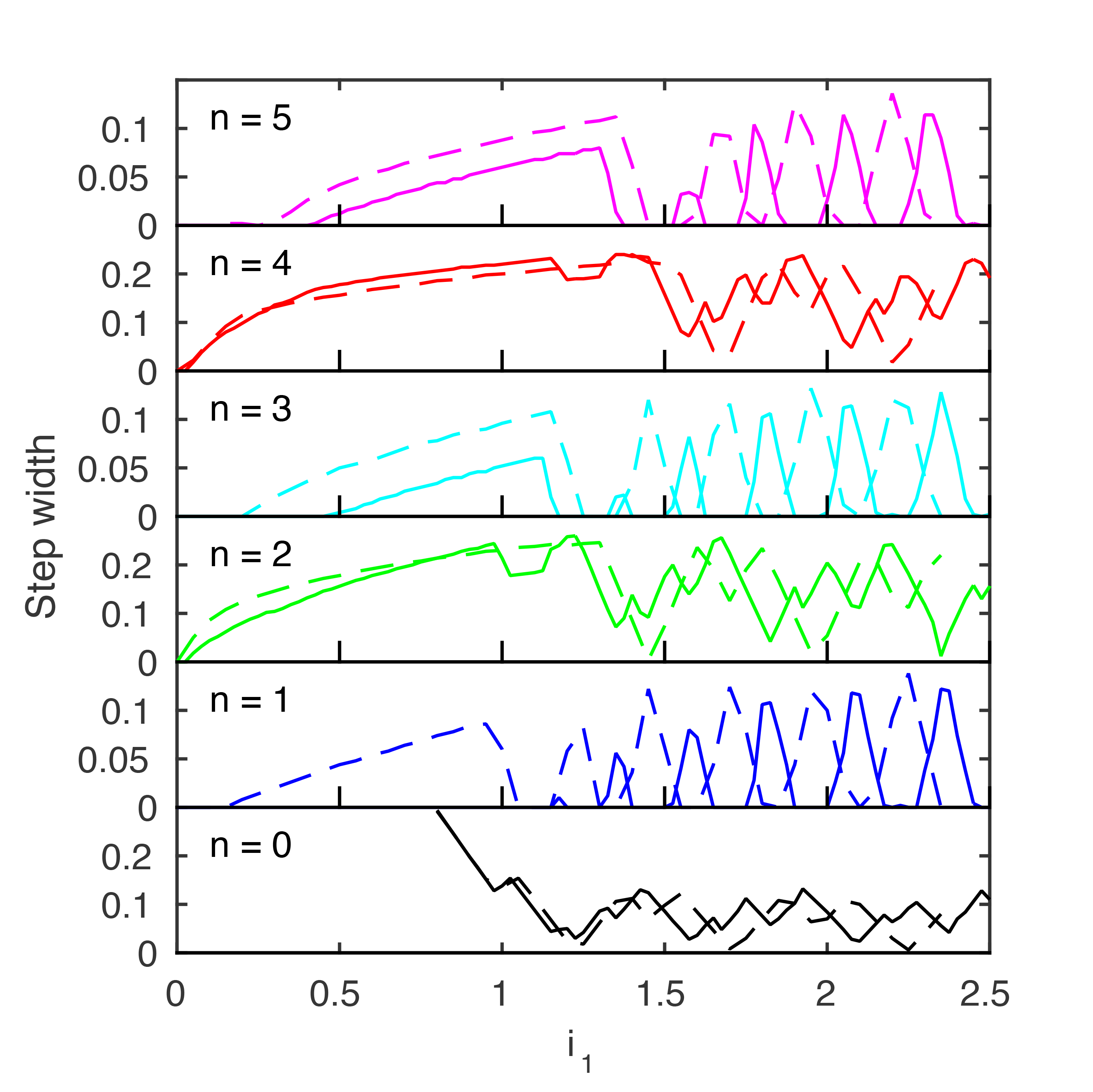
Figure 2: Calculated Shapiro step amplitudes as a function of $i_{1}$ for $\sigma\omega_{\mathrm{ac}}=0.1$ and $x=0.2$. The step amplitudes are normalized to the amplitude of the zeroth step at $i_{1}=0$. The dashed curves correspond to the RSJ model ($C=0$) and the solid curves to the RCSJ model with $\sigma=1$.

In the presence of MBS, the supercurrent can be roughly described by the sum of two contributions, $i_{\mbox{sc}}(\varphi)=i_{2\pi}\mathrm{sin}(\varphi)+i_{4\pi}\mathrm{sin}(\varphi/2)$, where the first term corresponds to the usual $2\pi$-periodic supercurrent and the second term is a $4\pi$-periodic contribution ($4\pi\mbox{SC}$), which arises in the presence of MBS. Henceforth, we will characterize the junction by the ratio $x\equiv i_{4\pi}/i_{2\pi}$. Note that by writing $i_{2\pi}$ and $i_{4\pi}$ as constant coefficients we neglect finite size effects, and all possible transitions towards the quasicontinuum.

The solution to Eq. 1 yields the induced voltage $v(t)\equiv d\varphi/dt=(I_{c}R\sigma)^{-1}V$. In absence of an ac bias, i.e: $i_{1}=0$, the voltage is a periodic function with frequency $\omega_{0}=\mathcal{h}v(t)\mathcal{i}$, where $\mathcal{h}\ldots\mathcal{i}$ denotes time averaging. For $i_{1}\neq 0$, the voltage is in general a quasiperiodic function of frequencies $\omega_{0}$ and $\omega_{\mathrm{ac}}$. When $\omega_{0}$ and $\omega_{\mathrm{ac}}$ are commensurate, the system is said to be in phase-lock, and the average voltage is a multiple of the ac bias frequency, i.e: $\mathcal{h}v(t)\mathcal{i}=n\omega_{\mathrm{ac}}$, $n=0,1,2,\ldots$ . In Fig. 1 (a) we have represented the average voltage $\mathcal{h}v(t)\mathcal{i}$ as a function of $i_{0}$ for for $\sigma=1$, $\omega_{\mathrm{ac}}=0.3$ and $i_{1}=0.75$. For a finite value of the ac bias amplitude $i_{1}$, the induced voltage develops plateaus called Shapiro steps, at integer multiples of $\omega_{\mathrm{ac}}$. Inside these plateaus, the voltage is phase-locked to the ac bias. Shapiro steps can be used to discriminate the presence of MBS, because in the case of a pure $4\pi$-periodic supercurrent, one would expect to observe only the Shapiro steps for $n$ even. We will show below how a finite capacitance can give rise to a more involved Shapiro step picture where odd steps may appear at $i_{2\pi}=0$. Quasiperiodic solutions correspond roughly to the linear sections  of the curve at high $i_{0}$. Alternatively, the periodicity can be studied directly from the Fourier spectrum of the signal. For the phase-locked regime, the spectrum is changed according to the step, as noted in Appendix A. For the quasiperiodic regime, the presence of a $4\pi\mbox{SC}$ induces new Fourier components at $\omega_{0}/2$. As an example, we show in Fig. 1 (c) and (d) the Fourier spectra for the two regimes.

III Shapiro Step Widths

Loosely speaking, the width of the $n$th Shapiro step as a function of the ac bias $i_{1}$ follows the shape of the $n$th Bessel function, as noted. However, in the presence of both $2\pi$ and $4\pi$-periodic contributions to the supercurrent, this profile is qualitatively modified (Domínguez et al., 2012). For the RSJ model, ($C=0$), in the low ac bias amplitude regime ($i_{1}\ll 1$), the odd steps are suppressed provided that $i_{1}\lesssim i_{4\pi}$ and $\sigma\omega_{\mathrm{ac}}=\hbar\Omega_{\mathrm{ac}}/2eI_{c}R\lesssim i_{4\pi}$. Furthermore, in the high ac bias amplitude regime ($i_{1}\gg 1$) the even steps show a beating pattern coming from the contribution of both supercurrent terms (Domínguez et al., 2017). This high ac bias amplitude behavior persists for intermediate values of the capacitance. This is the case of Fig. 2, where we show the Shapiro step width as a function of the ac bias amplitude $i_{1}$ for $\sigma=1$.

The presence of a finite capacitance modifies the Shapiro step widths drastically as the junction is taken into the underdamped regime, $\sigma\lesssim 1$, as noted in the Appendices B and C. In this regime, the range of frequencies where we observe only even steps has to be reconsidered. In addition to $\sigma\omega_{\mathrm{ac}}=\hbar\Omega_{\mathrm{ac}}/2eI_{c}R\lesssim i_{4\pi}$ we also require that $\omega_{\mathrm{ac}}^{2}=\hbar\Omega_{\mathrm{ac}}^{2}C/2eI_{c}\lesssim i_{4\pi}$. These conditions have been derived in the Appendix D from the effect of a $4\pi\mbox{SC}$ on the voltage output. Remarkably, the presence of capacitance extends considerably the condition $i_{1}\lesssim i_{4\pi}$, valid for the RSJ model. In Fig. 2 we have represented the width of the first five Shapiro steps for $x=0.2$ and $\omega_{\mathrm{ac}}=0.1$ for both the RCSJ model with $\sigma=1$ (solid curves) and the RSJ model (dashed curves). For $\sigma=1$, the first step vanishes for ac bias amplitudes up to $i_{1}\simeq 1.2$ much larger than the amplitude of the $4\pi\mbox{SC}$, $i_{4\pi}=0.175$. Hence, the underdamped junction is a useful platform for detecting MBS even when the $4\pi\mbox{SC}$ is a small fraction of the total supercurrent. In contrast to the RSJ model, the quenching of the odd steps depends on the step number: the third and fifth steps vanish only up to $i_{1}\simeq 0.5$. This occurs because, at higher voltages, the resistive term, which is proportional to the voltage, is of greater importance than the capacitive one. Hence, for higher steps the results for $\sigma=1$ and $\sigma\to\infty$ become more similar. These new conditions obtained from the RCSJ model have to be considered when estimating $i_{4\pi}$ from the disappearance of the odd Shapiro steps in experiments.

In order to have an intuition about how the capacitance modifies the odd step widths, we show in Fig. 3 (a), the step width of the first and third steps as a function of the damping parameter $\sigma$ for a value of the ac bias $i_{1}=0.75$ larger than the amplitude of the $4\pi\mbox{SC}$, $i_{4\pi}=0.175$. We see how decreasing $\sigma$ results in the suppression of the first step, while the third step vanishes for a smaller value of $\sigma$. In Fig. 3 (b) we have represented the step width as a function of the ratio $x=i_{4\pi}/i_{2\pi}$. The first step vanishes for $x\simeq 0.25$ while the third step requires $x\simeq 0.65$ to be suppressed.

Figure 3: (a) Odd step widths, $n=1$ (blue) and $n=3$ (cyan) as a function of the damping parameter $\sigma$ for $\omega_{\mathrm{ac}}=0.3$, $i_{1}=0.75$. (b) Step widths as a function of $x=i_{4\pi}/i_{2\pi}$ for $\sigma=0.65$. (c) Schematic phase diagram for the parameters $\sigma$ and $\omega_{\mathrm{ac}}$ in logarithmic scale. The dashed lines correspond to $\tilde{i}_{4\pi}=0.1$ and $\tilde{i}_{4\pi}=10$ (see text below) for $i_{4\pi}=1$. The yellow area corresponds to the $4\pi$-periodic regime. The blue area corresponds to the Bessel regime. The green area corresponds to the intermediate regime.

On the other hand, when these conditions are not satisfied, the presence of a finite $4\pi\mbox{SC}$ is not enough to suppress the odd steps. In Appendix E we obtain that for high ac bias amplitudes, such that

$$\tilde{i}_{1}\gg\omega_{\mathrm{ac}}^{-4},\,\,\,\,\,\tilde{i}_{1}\gg\omega_{\mathrm{ac}}^{-2}\sigma^{-2},$$ (2)

where $\tilde{i}_{1}=i_{1}(\omega_{\mathrm{ac}}\sqrt{\omega_{\mathrm{ac}}^{2}+\sigma^{2}})^{-1}$, the junction is weakly affected by the change in the periodicity of the supercurrent. Even for low ac bias amplitudes, if $\sigma\omega_{\mathrm{ac}}\gg 1$ or $\omega_{\mathrm{ac}}^{2}\gg 1$ most of the current will flow through the resistive and capacitive channels and the effect of the $4\pi\mbox{SC}$ on the odd steps will be minimal. If any of these four conditions is met, the junction is said to be in the Bessel regime. In this regime, the Shapiro step widths can be obtained analytically, as noted in the Appendix B.

In Fig. 3 (c) we have represented an schematic phase diagram for the RCSJ model with a $4\pi\mbox{SC}$ as a function of the parameters $\sigma$ and $\omega_{\mathrm{ac}}$. The yellow region corresponds to the regime where we expect the $4\pi\mbox{SC}$ to have a strong effect on the junction behavior, the $4\pi$-periodic regime. The blue region corresponds to the Bessel regime and the green region corresponds to the intermediate phase, where the odd steps are suppressed only for low ac bias amplitude. The approximate phase boundaries are determined by $\tilde{i}_{4\pi}=0.1$ and $\tilde{i}_{4\pi}=10$, where we have defined $\tilde{i}_{4\pi}=i_{4\pi}\left[\omega_{\mathrm{ac}}\sqrt{\omega_{\mathrm{ac}}^{2}+\sigma^{2}}\right]^{-1}$.

Another consequence of the presence of a finite capacitance is that the odd steps do not necessarily disappear even if $i_{2\pi}=0$, as illustrated by the results of Fig. 4. Odd steps may still appear as a consequence of subharmonic phase-locking. Subharmonic steps, such as in Fig. 4 are always of smaller width than the corresponding harmonic steps (Waldram et al., 1970). This type of behavior is known to happen in the RCSJ equation as a consequence of symmetry breaking in the non-linear supercurrent term. This possibility is shown explicitly to happen in the high ac-bias regime in Appendix E. In the RSJ limit, i.e: $C=0$, subharmonic phase-lock is rigorously forbidden (Waldram and Wu, 1982). Moreover, in the presence of strong step overlap, numerical results indicate that subharmonic steps are strongly quenched. Since step overlap occurs predominantly when $\sigma\omega_{\mathrm{ac}}\ll\tilde{i}_{1}^{2}$ (Kautz, 1996), subharmonic steps seldom appear in the $4\pi$-periodic regime as defined above.

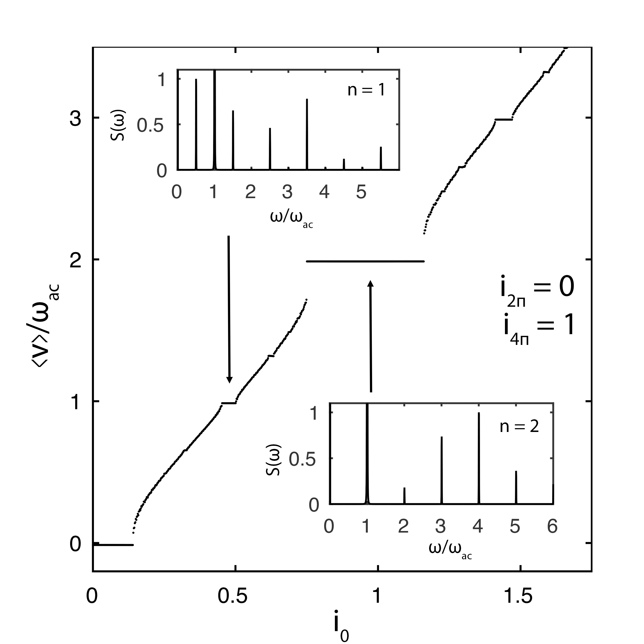
Figure 4: Shapiro step curve for $i_{2\pi}=0$ and $i_{4\pi}=1$ ($x\to\infty)$. Insets: Fourier spectrum obtained numerically at the first and second steps. The Fourier spectrum in the first step consists only of half-harmonic components plus a component at $\omega_{\mathrm{ac}}$, while the Fourier spectrum at the second step consists only of components at integer multiples of $\omega_{\mathrm{ac}}$, in accordance with the analytical results of Appendix E. Parameters considered: $\omega_{\mathrm{ac}}=1.6$, $\sigma=0.3$, $\tilde{i}_{1}=10$.

IV Emission Spectrum Analysis

The periodicity of the response can be studied through the frequency spectra, $S_{\omega}=|v(\omega)|$, where $v(\omega)$ is the Fourier transform of the signal obtained in a Shapiro experiment. The emission spectrum of the voltage was obtained in Ref. (Deacon et al., 2016) from experiments on a topological junction, in order to probe the phase dependent periodicity of the junction as a function of the dc-current bias, $i_{0}$. Below, we will analyze in detail the Fourier spectrum of the voltage in the presence of both dc and ac bias: $i_{\mathrm{dr}}(t)=i_{0}+i_{1}\mathrm{sin}(\omega_{\mathrm{ac}}t)$. We consider the Fourier spectrum of both phase-locked and quasiperiodic solutions.

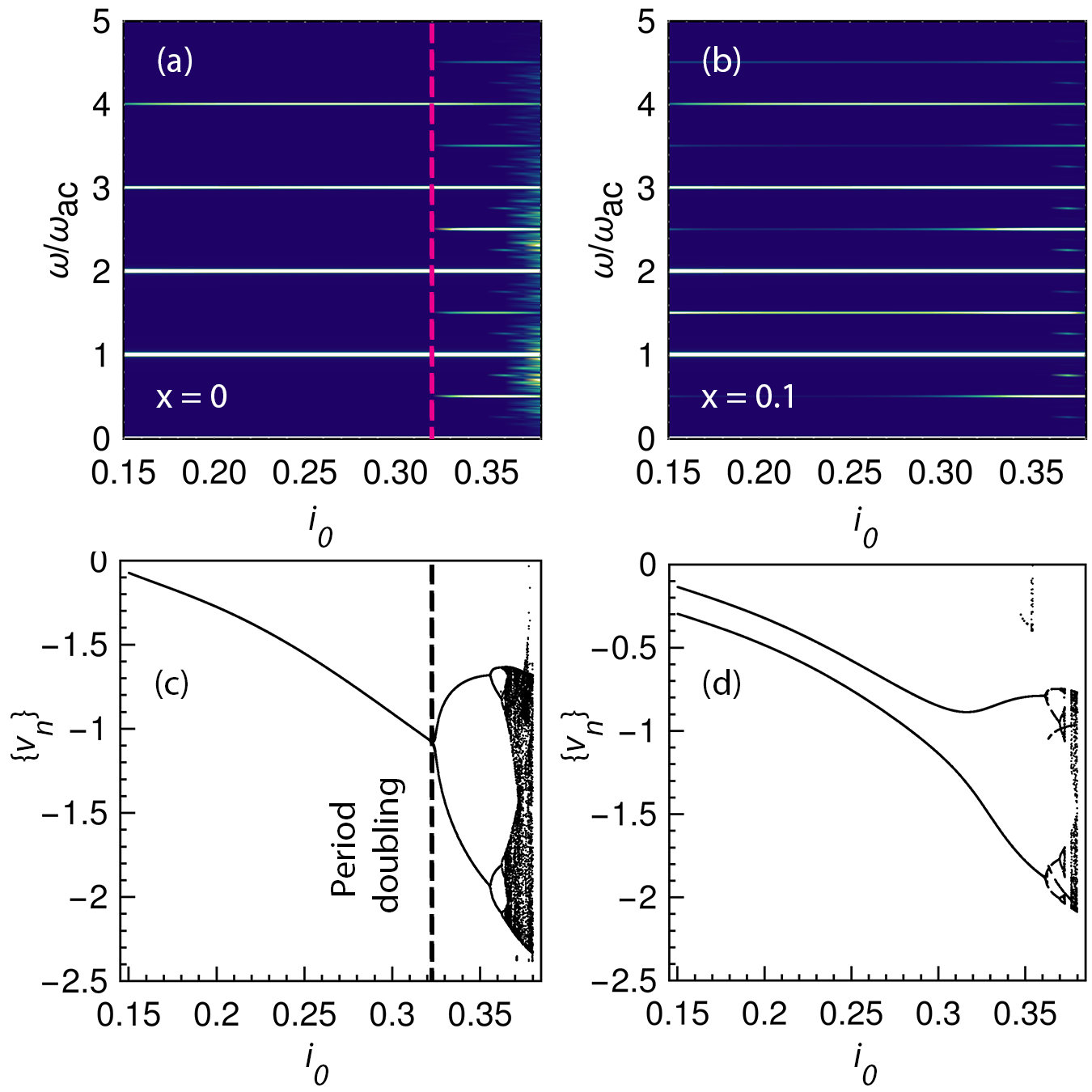
Figure 5: (a) Density plot of the Fourier transform of the voltage signal $v(\omega)$ for $\sigma=0.3$, $\omega_{\mathrm{ac}}=0.6$, $x=0$ and (b) $x=0.1$. (c) Bifurcation diagram for $\sigma=0.3$, $\omega_{\mathrm{ac}}=0.6$ and $x=0$ and (d) $x=0.1$. Period doubling results in the appearance of a subharmonic response even when $i_{4\pi}=0$, which may hide the presence of a $4\pi\mbox{SC}$. It appears as a pitchfork bifurcation at $i_{0}\simeq 0.32$ in (c). The point at which this occurs has been marked with a dashed magenta line.

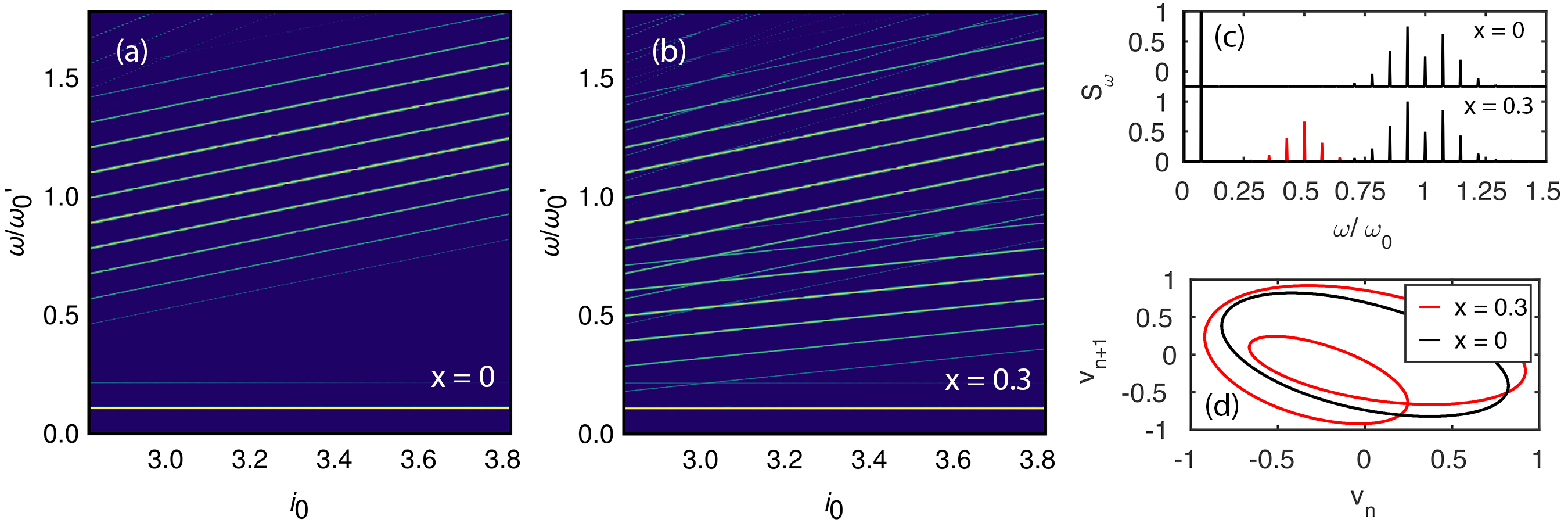
Figure 6: (a), (b) Density plot of $\mbox{ln}[S_{\omega}(i_{0})]$ for $\omega_{\mathrm{ac}}=0.3$ and $i_{1}=0.58$, with a $4\pi$-periodic contribution of $x=0$ and $x=0.3$, respectively. In both cases, the frequency axis is normalized to the natural frequency at the lowest value of $i_{0}$; that is, $\omega_{0}^{\prime}=\omega_{0}(2.82)$ (c) Fourier spectrum for the same parameters as in (a) without a $4\pi\mbox{SC}$ (up) and with a $4\pi\mbox{SC}$ of $x=0.3$ (down), corresponding to $i_{0}=3.62$. The peaks corresponding to the natural frequency and half of the natural frequency have been indicated; the peaks originating from the $4\pi$-periodic contribution are marked in red. (d) First return map (FRM) for the same parameters as in (c) with black indicating the FRM for $x=0$ and red indicating the FRM for $x=0.3$.

IV.1 Shapiro steps: period doubling

The typical voltage response in the phase-locked regime of a topologically trivial Josephson junction exhibits peaks at integer values of the ac bias frequency, that is, at $\omega=k\omega_{\mathrm{ac}}$, $k\mathcal{2}\mathbb{Z}$. However, for a finite $4\pi\mbox{SC}$, the voltage response inside a given odd step is necessarily $4\pi$-periodic, as shown in Appendix A, while the even steps remain unaltered. This is shown, for example, in the insets of Fig. 4. The time evolution of the voltage on the $n$th odd Shapiro step can be expressed as a Fourier series

$$v(t)=\sum_{l=0}^{\infty}v_{l}\mbox{e}^{i(l/2)\omega_{\mathrm{ac}}t},$$ (3)

where $v_{0}=n\omega_{\mathrm{ac}}$. Then, the periodicity of the voltage can be extracted from the emission spectrum. However, in a capacitively-shunted junction, the non-linear dynamics can break the symmetry of the RCSJ equation of motion. Then, even in absence of $4\pi\mbox{SC}$, i.e: $x=0$, the steps may develop spontaneously a subharmonic response at half the ac bias frequency, and thus the Fourier spectrum shows peaks at integer multiples of $\omega_{\mathrm{ac}}/2$. This phenomenon is called period doubling. It has been studied in the past (Kautz and Monaco, 1985; Kautz, 1987) in the context of the onset of chaos in the RCSJ model (Pedersen et al., 1980).

In Fig. 5 (a) and (b) we illustrate the Fourier spectrum $v(\omega)$ as a function of $i_{0}$ for $x=0$ and $x\neq 0$. In the interval $i_{0}\mathcal{2}[0.15,0.32]$, we observe a set of resonances placed at integer multiples of the frequency $\omega_{\mathrm{ac}}$ ($\omega_{\mathrm{ac}}/2)$ for $x=0$ ($x\neq 0$). In contrast, for $i_{0}>0.32$, the system becomes unstable and the response becomes $4\pi$-periodic even for $x=0$, as the system enters in a resonance at half the plasma frequency of the junction (Kautz and Monaco, 1985).

The period doubling of a phase-locked solution manifests itself as a pitchfork bifurcation inside the steps, whereas for a junction with $i_{4\pi}\neq 0$ the whole step is $4\pi$-periodic. This is represented in Fig. 5 (c) and (d), where we have plotted for each value of $i_{0}$ the voltage at different periods; that is, for each $i_{0}$, we have plotted the set $\{v(t_{i})\}$, where $t_{i+1}=t_{i}+2\pi/\omega_{\mathrm{ac}}$. For a $2\pi$-periodic signal, to each $i_{0}$ corresponds a single value $v(t_{i})$, whereas for a $4\pi$-periodic signal, to each $i_{0}$ corresponds two values $\{v(t_{i}),v(t_{i}+2\pi/\omega_{\mathrm{ac}})\}$. The dense black portions of the diagram correspond to aperiodic solutions. For $x\neq 0$, the whole step is $4\pi$-periodic, whereas for $x=0$, the step is $4\pi$-periodic starting at the resonance at $i_{0}=0.32$. Then, the experimental distinction between $x=0$ and $x\neq 0$ requires determining whether or not there is a peak in the Fourier spectrum at $3\omega_{\mathrm{ac}}/2$ in the region $i_{0}\mathcal{2}[0.15,0.32]$.

In Ref. (Kautz, 1996), the authors propose a condition for avoiding period doubling, namely that the ac bias amplitude is large enough that $\tilde{i}_{1}\gg\omega_{\mathrm{ac}}^{-4}$. Since this corresponds to the Bessel regime, where we do not expect a large $4\pi$-periodic response, the possibility of period doubling cannot be neglected in the parameter regions where the junction is strongly $4\pi$-periodic.

IV.2 Quasiperiodic regime

In order to explore other regimes, we may look instead at quasiperiodic (QP) solutions appearing at $i_{0}\gg\omega_{\mathrm{ac}}\sigma\tilde{i}_{1}$ (Kautz, 1996). When the natural frequency of the junction $\omega_{0}=\sigma^{-1}i_{0}$ and the driving frequency $\omega_{\mathrm{ac}}$ are incommensurate, the voltage response is quasiperiodic. This is the case in the apparently continuous, linear parts of the $i_{0}-\mathcal{h}v\mathcal{i}$ curves, as indicated in Fig. 1 (a), where the Shapiro steps are small and the current follows the current-voltage characteristic. The voltage response curve in the quasiperiodic regime of a Josephson junction can be written as a generalized Fourier series (Schilder et al., 2006)

$$v(t)=\overset{\infty}{\underset{k,l=0}{\sum}}v_{kl}e^{i(k\omega_{\mathrm{ac}}+l\omega_{0}/2)t},$$ (4)

where $v_{kl}=\omega_{0}$. In the Fourier spectrum for $x=0$, shown in Fig. 6 (a), there is a resonance at $\omega_{\mathrm{ac}}$, corresponding to the ac bias and another at $\omega_{0}$, corresponding to the intrinsic frequency of the junction. Then, starting from $\omega_{0}$, another set of peaks appears separated from $\omega_{0}$ an integer multiple of $\omega_{\mathrm{ac}}$. The Fourier spectrum for the case $x\neq 0$, represented in Fig. 6 (a) exhibits an extra resonance at $\omega_{0}/2$ plus a new set of satellite peaks once again separated an integer multiple of $\omega_{\mathrm{ac}}$.

The presence of a $4\pi\mbox{SC}$ can also be observed through the first-return maps (FRMs), as these are heavily modified by change in the periodicity of the supercurrent terms. A FRM is composed of pairs $\{v(t_{i+1}),v(t_{i})\}$, where $t_{i+1}=t_{i}+2\pi/\omega_{\mathrm{ac}}$. The FRMs are sensitive to the periodicity of the voltage response, in a similar way to Poincaré maps (Luo et al., 1998b). The FRMs, however, can be obtained from a time resolved scalar response, like the voltage signal of a typical Josephson junction experiment. For a $2\pi$-periodic voltage response, the FRMs are ellipses, as can be seen in Fig. 6 (d). As the periodicity of the response shifts to $4\pi$, however, the ellipses twist inward and self-crossings appear, as represented in Fig. 6 (d) for different values of $i_{0}$. This is in accordance with the scenario observed in the FRMs of superlattice current self-oscillations by Luo et al (Luo et al., 1998b).

Both the changes to the Fourier spectra and to the FRMs of quasiperiodic solutions due to a finite $4\pi SC$ are a general behavior when sufficiently away from the steps, and thus can be used to discern the topological nature of the junction. Close to the steps, the solutions may be heavily distorted, exhibiting high subharmonic response or even fractal structure in their FRMs (Bulashenko et al., 1999; Sánchez et al., 2001).

V Conclusions

We have explained theoretically the experimental features observed in a Josephson junction in the presence of a $4\pi\mbox{SC}$ by introducing a capacitance term in the semiclassical equation of motion of the junction. Namely, we have shown that in the underdamped regime, i.e: when the capacitive term is stronger than the resistive one, the odd steps are suppressed even for high ac bias amplitudes. Furthermore, we observe an uneven quenching, with the first Shapiro step being more affected by the presence of a $4\pi\mbox{SC}$ than the subsequent odd steps. This behavior reproduces qualitatively the experimental results published so far, and indicates that for a correct estimation of the $4\pi\mbox{SC}$ amplitude it is necessary to consider the presence of a finite capacitance in the junction.

We also consider the possibility to study the periodicity of the junction through the Fourier spectrum of the voltage response. We show how the appearance of period doubling bifurcations in the regions where the $4\pi$-periodic response is at its largest may difficult this observation in the phase-locked regime, corresponding to the Shapiro steps. The Fourier spectrum of quasiperiodic solutions also provides information about the topology of the junction. While far from the step regions, the quasiperiodic response is surprisingly stable and shows the marks of a finite $4\pi$-periodic response in its Fourier components. The corresponding first-return maps are twisted, compared to the ellipses found for the $2\pi$-periodic case. This may be used to discern the periodicity of the junction directly from the voltage response.

Overall, we have analyzed both the phase-locked and the quasiperiodic regimes of the topological RCSJ model, showing how each may be used to help in the detection of Majorana bound states. Furthermore, the results shown here for the RCSJ model may be useful to understand the process of periodicity change in other non-linear systems.

Appendix A Subharmonic response in the $4\pi$-periodic Josephson junction.

Phase lock occurs when the phase advances by $2\pi l$ after $m$ periods $T=2\pi/\omega_{\mathrm{ac}}$ of the ac driving

$$\varphi\left(t+mT\right)=\varphi(t)+2\pi l$$ (5)

for integers $l,m$. The Josephson equations predicts for that case $\mathcal{h}v\mathcal{i}=\left\langle\mbox{d}\varphi/\mbox{d}t\right\rangle=(l/m)\omega_{\mathrm{ac}}$. When $m>1$ and $l/m$ is not an integer, the junction may develop subharmonic phase-lock, observed as steps corresponding to fractions of the ac bias frequency. Subharmonic phase-locking is forbidden in the RSJ limit (Waldram and Wu, 1982).

If the odd steps do not vanish completely, the voltage response inside a given odd step will have twice the period of the ac bias, that is, it will have $m=2$ in Eq. (5). The voltage response corresponding to the first step may be $4\pi$-periodic and still contribute to the step, provided that $\varphi\left(t+2T\right)=\varphi(t)+4\pi$. In fact, as we will show now, the response inside a given odd step must be $4\pi$-periodic.

Consider a $2\pi$-periodic trial solution for the $n$th step of the form

$$\varphi(t)=\varphi_{0}+n\omega_{\mathrm{ac}}t-\sum_{l=1}^{\infty}\tilde{i}_{l}\mathrm{sin}\left(l\omega_{\mathrm{ac}}t+\theta_{l}\right),$$ (6)

with $n\mathcal{2\mathbb{Z}}$. Substituting Eq. (6) into the RCSJ equation one obtains a complicated formula for the free parameters $\varphi_{0},\{\tilde{i}_{l},\theta_{l}\}$. This can be solved in particular limits, to yield analytical expressions for these parameters, as detailed below. Here, instead, we integrate all terms in the RCSJ equation over one period of the ac bias, obtaining

$$\begin{array}[]{c}i_{4\pi}\sum_{\mathbf{k}}\frac{2}{\left(\sum_{l}lk_{l}-\frac{n}{2}\right)\omega_{\mathrm{ac}}}\left[\prod_{l}J_{k_{l}}\left(\frac{\tilde{i}_{l}}{2}\right)\right]\\ \times\mathrm{sin}\left[\left(\sum_{l}lk_{l}-\frac{n}{2}\right)\pi+\frac{\varphi_{0}}{2}-\sum_{l}k_{l}\theta_{l}\right]\\ \times\mathrm{sin}\left[\left(\sum_{l}lk_{l}-\frac{n}{2}\right)\pi\right]=0,\end{array}$$ (7)

where $J_{n}(x)$ is the $n$th order Bessel function and $\mathbf{k}=(k_{1},k_{2},\ldots)$ is a vector of indices, each running from $-\infty$ to $\infty$. Note that the sine factor multiplying the left-hand side is

$$\mathrm{sin}\left[\left(\sum_{l}lk_{l}-\frac{n}{2}\right)\pi\right]=\left\{\begin{array}[]{c}0\,\,\,\mbox{if }n\mbox{ is even}\\ 1\,\,\,\mbox{if }n\mbox{ is odd}\end{array}\right.$$ (8)

Thus, Eq. (7) indicates that in the odd steps the RCSJ equation cannot be satisfied if the solution is $2\pi$-periodic even on average over a period. In order to obtain a satisfactory solution for the RCSJ equation on an odd step, we need to take into account the possibility of a subharmonic response, and include terms at frequencies $l\omega_{\mathrm{ac}}/2$, $l\mathcal{2}\mathbb{Z}$.

Figure 7: Washboard potential for $x=0$ (dashed lines) and $x=0.2$ (full lines). The shape of the potential shifts its periodicity as the $4\pi$-periodic contribution increases in importance. The result is two subsets of wells: one consisting of shallow wells and another of deep wells.

This can be understood by using the mechanical analogue of the RCSJ equation, that is, by considering the RCSJ equation as representing the motion of a massive particle under a washboard potential

$$u(\varphi)=i_{2\pi}\mathrm{cos}(\varphi)+i_{4\pi}\mathrm{cos}(\varphi/2)$$ (9)

with damping given by $\sigma\mbox{d}\varphi/\mbox{d}t$ and both a constant force $i_{0}$ and a time-dependent force $i_{1}\mathrm{sin}(\omega_{\mathrm{ac}}t)$. The washboard potential looks like a sequence of potential wells, as represented in Fig. 7. For a small value of $x$, there are two types of wells with different heights, so that a shallow well is followed by a deep well and vice versa. For an odd step, the “particle” traverses an odd number of wells each ac bias period. Hence after an ac bias period it moves from a shallow well into a deep well, and it takes it another period to move from a deep well back into a shallow well. For a particle in an odd step, the potential appears $4\pi$-periodic, since it takes two periods to go back to the initial position. In the case of an even step, where the particle traverses an even number of wells each ac bias period, after a cycle it ends its movement in the same type of well it started. For a particle in an even step, the potential appears $2\pi$-periodic. The voltage response in an odd step, will develop a $4\pi$-periodic voltage response, as it requires two ac bias periods for the particle to turn back to the well where it started. In that sense, the remainder in Eq. (7) acts like an impulse per ac bias period on the particle which will tend to make its movement $4\pi$-periodic if the particle is in an odd step, and will have no effect if the particle is in an even step.

Appendix B Phase-lock in the Bessel regime

In this section, we obtain analytical expressions for the step widths inside the Bessel regime. In that case, the voltage response to the applied current bias may be approximated as linear $v(t)=v_{0}-v_{1}\mathrm{cos}(\omega_{\mathrm{ac}}t)$, with $n\mathcal{2\mathbb{Z}}$. In that case, one obtains a trial phase-locked solution $\varphi(t)=\varphi_{0}+v_{0}t-\tilde{i}_{1}\mathrm{sin}(\omega_{\mathrm{ac}}t+\theta_{1})$, where $\tilde{i}_{1}=v_{1}/\omega_{\mathrm{ac}}$. Note that, as explained above, this solutions cannot be exact for an odd step, and a $4\pi$-periodic term needs to be added. We will consider this problem in Appendix E.

Starting from $\varphi(t)$, one can calculate the amplitude of the steps in the Bessel regime (Kautz, 1996) by substituting $\varphi(t)$ and solving for $\varphi_{0}$. To do so, we equate the constant terms at both sides of the RCSJ equation with $\varphi(t)$ substituted on it. Substitution inside the supercurrent terms gives, according to the Jacobi-Anger expansion

$$\begin{array}[]{c}i_{\mathrm{sc}}(t)=i_{2\pi}\sum_{l=-\infty}^{\infty}J_{l}(\tilde{i}_{1})\mathrm{sin}[(v_{0}-l\omega_{\mathrm{ac}})t+\varphi_{0}-l\theta_{1}]\\ +i_{4\pi}\sum_{l=-\infty}^{\infty}J_{l}(\tilde{i}_{1}/2)\mathrm{sin}[(v_{0}/2-l\omega_{\mathrm{ac}})t+\varphi_{0}/2-l\theta_{1}].\end{array}$$ (10)

If $v_{0}\neq n\omega_{\mathrm{ac}}$, with $n$ an integer, the supercurrent has no constant term. Equating the constant terms from the rest of the RCSJ equation yields $v_{0}=i_{0}\sigma^{-1}$, indicating that the voltage follows the resistive line $V=IR$. However, if $v_{0}=n\omega_{\mathrm{ac}}$ –that is, at the values that we expect Shapiro steps to appear–, the supercurrent term contributes to the average voltage. For a Shapiro step corresponding to $n$ odd, when $v_{0}=n\omega_{\mathrm{ac}}$ we obtain

$$n\sigma\omega+i_{2\pi}J_{n}(\tilde{i}_{1})\mathrm{sin}\varphi_{n}=i_{0},$$ (11)

where $\varphi_{n}=\varphi_{0}-n\theta_{1}$. This equation fixes the free parameter $\varphi_{0}$. The interesting aspect of this relation is that it is satisfied for a range of $i_{0}$ of

$$(\Delta i_{0})_{n}^{\mathrm{odd}}=2i_{2\pi}|J_{n}(\tilde{i}_{1})|$$ (12)

resulting in the appearance of a step at height $n\omega_{\mathrm{ac}}$, as observed experimentally.

It remains to determine $\tilde{i}_{1}$ and $\theta_{1}$. To obtain expressions for them one looks at the Fourier components at a frequency of $\omega_{\mathrm{ac}}$. Ignoring the contribution from the terms $\mathrm{sin}(\varphi)$ and $\mathrm{sin}(\varphi/2)$, one obtains approximate expression for $\tilde{i}_{1}$ and $\theta_{1}$

$$\tilde{i}_{1}=\frac{i_{1}}{\omega_{\mathrm{ac}}\sqrt{\omega_{\mathrm{ac}}^{2}+\sigma^{2}}},$$ (13)

$$\theta_{1}=\mathrm{arctan}(\sigma/\omega_{\mathrm{ac}}).$$ (14)

As explained below, the approximation of neglecting the supercurrent is justified provided that we stay in the Bessel regime. Even outside, these definitions provide a satisfactory descriptions of the dependance of $\tilde{i}_{1}$ and $\theta_{1}$ on $\omega_{\mathrm{ac}}$ and $\sigma$.

For the even steps, the analogue of Eq. (11) is

$$\begin{array}[]{c}n\omega\sigma+i_{2\pi}J_{n}(\tilde{i}_{1})\mathrm{sin}\varphi_{n}\\ +i_{4\pi}J_{\frac{n}{2}}\left(\frac{\tilde{i}_{1}}{2}\right)\mathrm{sin}\left(\frac{1}{2}\varphi_{n}\right)=i_{0}\end{array}$$ (15)

and the step width of the even steps is

$$\begin{array}[]{c}(\Delta i_{0})_{n}^{\mathrm{even}}=2\mathrm{max}_{\varphi_{n}}\left[i_{2\pi}J_{n}(\tilde{i}_{1})\mathrm{sin}\varphi_{n}+\right.\\ \left.i_{4\pi}J_{\frac{n}{2}}\left(\frac{\tilde{i}_{1}}{2}\right)\mathrm{sin}\left(\frac{1}{2}\varphi_{n}\right)\right].\end{array}$$ (16)

Except for the renormalization of $\tilde{i}_{1}$, these results are consistent with those obtained in Ref. (Domínguez et al., 2017) within the RSJ model, suggesting that the effect of capacitance is not so important within the Bessel regime. Eq.  12 indicates that the odd steps disappear at $i_{2\pi}=0$, while, according to Eq. 16, the even steps do not vanish as the contribution coming from the $\propto i_{4\pi}$ term compensates the decrease in the contribution from the $\propto i_{2\pi}$ term. However, this trial solution neglects the fact that the voltage response in an odd step has to be $4\pi$-periodic. In Appendix E we will see that in the correct description (i.e: with a $4\pi$-periodic voltage response) the odd steps have a finite width and hence do not disappear completely.

Appendix C Outside the Bessel regime: step width

In this appendix we extend the results of the previous section to parameter regions far from the Bessel regime. Here we cannot obtain analytical results except for certain limits, but the trial function method can be used to gain insight on the junction behavior.

In order to study these effects, we study a quasiperiodic solution of the type

$$\varphi(t)=\varphi_{0}+v_{0}t-\sum_{j,l=-\infty}^{\infty}\tilde{i}_{jl}\mathrm{sin}\left[\xi_{jl}t+\theta_{jl}\right],$$ (17)

where $\xi_{jl}=\left(jv_{0}/2+l\omega_{\mathrm{ac}}\right)$. We also require that $\tilde{i}_{jl}=0$ if $\xi_{jl}=0$. Here, if $i_{4\pi}=0$ then $j$ is restricted to even numbers. This type of trial solution replicates correctly the numerical results which show that the odd steps develop a half harmonic response (i.e: the voltage response is $4\pi$-periodic) whereas the even steps only exhibit integer harmonics. We delay a proper justification for this trial function until the end of this section.

After inserting $\varphi(t)$ into the RCSJ equation, the supercurrent is given by

$$\begin{array}[]{c}i_{\mbox{sc}}(t)=i_{2\pi}\sum_{\mathbf{k}}\mathcal{J}_{\mathbf{k}}(\tilde{\mathbf{i}})\mathrm{sin}\left[\varphi_{0}+\left(v_{0}-\mathbf{k}\cdot\boldsymbol{\xi}\right)t-\mathbf{k}\cdot\boldsymbol{\theta}\right]\\ +i_{4\pi}\sum_{\mathbf{k}}\mathcal{J}_{\mathbf{k}}(\tilde{\mathbf{i}}/2)\mathrm{sin}\left[\varphi_{0}/2+\left(v_{0}/2-\mathbf{k}\cdot\boldsymbol{\xi}\right)t-\mathbf{k}\cdot\boldsymbol{\theta}\right],\end{array}$$ (18)

where

$$\mathcal{J}_{\mathbf{k}}(\tilde{\mathbf{i}})=\prod_{j,l}J_{k_{jl}}\left(\tilde{i}_{jl}\right)$$ (19)

is a generalized Bessel function, $\mathbf{k}=(k_{ij})$ is a matrix of indices and the sum is over all possible $\mathbf{k}$, with each $k_{jl}$ going from $-\infty$ to $+\infty$. Similarly, $\tilde{\mathbf{i}}=(\tilde{i}_{ij})$ is a matrix of the Fourier amplitudes. We define in a similar way $\boldsymbol{\xi}$ and $\boldsymbol{\theta}$. The dot indicates the Frobenius inner product of matrices $\mathbf{a}\cdot\mathbf{b}=\sum_{jl}a_{jl}b_{jl}$.

In a similar way to the Bessel regime, Shapiro steps appear around certain values $v_{0}$ of the average voltage, satisfying

$$\begin{array}[]{c}v_{0}-2\boldsymbol{\kappa}\cdot\boldsymbol{\xi}=0\\ v_{0}-\boldsymbol{\kappa}^{\prime}\cdot\boldsymbol{\xi}=0\end{array}$$ (20)

for a set of indices $\{\kappa_{ij}\}$ and $\{\kappa_{ij}^{\prime}\}$ running from $-\infty$ to $+\infty$. The first (second) equation appears as a result of the $2\pi$-periodic ($4\pi$-periodic) supercurrent element. In terms of the ac bias frequency, steps appear at values $v_{0}$ of the average voltage given by

$$v_{0}=2\omega_{\mathrm{ac}}\frac{\sum_{j,l}\kappa_{jl}l}{2-\sum_{j,l}\kappa_{jl}j},$$ (21)

$$v_{0}=2\omega_{\mathrm{ac}}\frac{\sum_{j,l}\kappa_{jl}^{\prime}l}{1-\sum_{j,l}\kappa_{jl}^{\prime}j}.$$ (22)

Note that the $\{\kappa_{l,j}\}$ and $\{\kappa_{l,j}^{\prime}\}$ coefficients must be the same in both the denominator and the numerator. If $i_{2\pi}=0$, then steps appear only at the values of $v_{0}$ given by Eq. (22). In that case, there is no reason to expect the odd steps to disappear for a trial solution like Eq. (17). If $1-\sum_{j,l}\kappa_{jl}^{\prime}j$ is even, then Eq. (22) indicates that there will be odd steps. This is the case represented in Fig. 4.

The step width for a certain $v_{0}$ is obtained by finding the range of $i_{0}$ for which there is a $\varphi_{0}$ that satisfies

$$\begin{array}[]{c}\sigma v_{0}+i_{2\pi}\sum_{\boldsymbol{\kappa}}\mathcal{J}_{\boldsymbol{\kappa}}(\tilde{\mathbf{i}})\mathrm{sin}\left[\varphi_{0}-\boldsymbol{\kappa}\cdot\boldsymbol{\theta}\right]\\ +i_{4\pi}\sum_{\boldsymbol{\kappa}^{\prime}}\mathcal{J}_{\boldsymbol{\kappa}^{\prime}}(\tilde{\mathbf{i}}/2)\mathrm{sin}\left[\frac{\varphi_{0}}{2}-\boldsymbol{\kappa}^{\prime}\cdot\boldsymbol{\theta}\right]=i_{0},\end{array}$$ (23)

with $\boldsymbol{\kappa}$ and $\boldsymbol{\kappa}^{\prime}$ given by Eqs. (21) and 22.

Appendix D Outside the Bessel regime: Fourier components

In this appendix we take the results of the previous section and focus on the response inside a given odd step. For an even step, the trial solution in Eq. (17) only has integer components. For an odd step, the trial solution has integer and half-integer harmonics, yielding

$$\varphi(t)=\varphi_{0}+n\omega_{\mathrm{ac}}t-\sum_{l=1}^{\infty}\tilde{i}_{l/2}\mathrm{sin}\left(\frac{l\omega_{\mathrm{ac}}}{2}t+\theta_{l/2}\right).$$ (24)

Then, the RCSJ equation becomes a set of equations for each pair of Fourier amplitudes and phases $\{\tilde{i}_{l/2},\theta_{l/2}\}$. Then, the previously defined $\mathbf{k},\tilde{\mathbf{i}},\boldsymbol{\theta},\boldsymbol{\xi}$ are vectors in the index $l$, so that, for example: $\mathbf{k}=(k_{1},k_{2},\ldots)$ We need these Fourier coefficients in order to obtain the step width from Eq. (23). In particular, for the Fourier component at the frequency $m\omega_{\mathrm{ac}}/2$, there are two equations.

$$\begin{array}[]{c}i_{2\pi}\sum_{\tilde{\mathbf{k}},s_{1}}s_{1}\mathcal{J}_{\tilde{\mathbf{k}}}(\tilde{\mathbf{i}})\mathrm{cos}\left(\varphi_{0}-\tilde{\mathbf{k}}\cdot\boldsymbol{\theta}\right)\\ +i_{4\pi}\sum_{\tilde{\mathbf{k}}^{\prime},s_{1}}s_{1}\mathcal{J}_{\tilde{\mathbf{k}}^{\prime}}(\tilde{\mathbf{i}}/2)\mathrm{cos}\left(\varphi_{0}/2-\tilde{\mathbf{k}}^{\prime}\cdot\boldsymbol{\theta}\right)\\ +\frac{m}{2}\omega_{\mathrm{ac}}\sigma\tilde{i}_{m/2}\mathrm{sin}\left(\theta_{m/2}\right)+\frac{m^{2}}{4}\omega_{\mathrm{ac}}^{2}\tilde{i}_{m/2}\mathrm{cos}\left(\theta_{m/2}\right)=i_{1}\delta_{m,2},\end{array}$$ (25)

$$\begin{array}[]{c}i_{2\pi}\sum_{\tilde{\mathbf{k}},s_{1}}\mathcal{J}_{\tilde{\mathbf{k}}}(\tilde{\mathbf{i}})\mathrm{sin}\left(\varphi_{0}-\tilde{\mathbf{k}}\cdot\boldsymbol{\theta}\right)\\ +i_{4\pi}\sum_{\tilde{\mathbf{k}}^{\prime},s_{1}}\mathcal{J}_{\tilde{\mathbf{k}}^{\prime}}(\tilde{\mathbf{i}}/2)\times\mathrm{sin}\left(\varphi_{0}/2-\tilde{\mathbf{k}}^{\prime}\cdot\boldsymbol{\theta}\right)\\ -\frac{m}{2}\omega_{\mathrm{ac}}\sigma\tilde{i}_{m/2}\mathrm{cos}\left(\theta_{m/2}\right)+\frac{m^{2}}{4}\omega_{\mathrm{ac}}^{2}\tilde{i}_{m/2}\mathrm{sin}\left(\theta_{m/2}\right)=0\end{array}$$ (26)

with the term $i_{1}\delta_{m,2}$ coming from the ac bias. Here $s_{1}=\pm 1$, and the sum is over the values $\{\tilde{\mathbf{k}},\tilde{\mathbf{k}}^{\prime}\}$ that satisfy

$$\begin{array}[]{c}s_{1}m+\sum_{l}l\tilde{k}_{l}=2n,\\ s_{1}m+\sum_{l}l\tilde{k}_{l}^{\prime}=n,\end{array}$$ (27)

corresponding to the terms proportional to $i_{2\pi}$ and to $i_{4\pi}$, respectively.

If we follow the prescription given in the definition of $\tilde{i}_{1}$ and $\theta_{1}$ in Appendix B, we would neglect the two sums coming from the supercurrent terms, and then we would find the trivial solution $\tilde{i}_{m/2}=0$ for $m\neq 2$ and we recover the expressions for $\tilde{i}_{1}$ and $\theta_{1}$ inside the Bessel regime, Eqs. (13) and (14). Since this prescription is not valid whenever $\omega_{\mathrm{ac}}\sigma$ or $\omega_{\mathrm{ac}}^{2}$ are comparable to $i_{2\pi}$ or $i_{4\pi}$, and $i_{2\pi}+i_{4\pi}\simeq 1$, we obtain the previously stated result that the system responds linearly to the applied bias whenever $\omega_{\mathrm{ac}}^{2}\gg 1$ or $\omega_{\mathrm{ac}}\gg 1/\sigma$.

The $4\pi$-periodic supercurrent term has a strong effect on the step widths when the terms it generates in Eqs. (25) and (26) are comparable to the rest of the terms. That is

$$\omega_{\mathrm{ac}}\sigma\lesssim i_{4\pi},\,\omega_{\mathrm{ac}}^{2}\lesssim i_{4\pi},$$ (28)

At this point we can justify the choice of trial solution, Eq. (17), and in particular the choice of the periodic part. Other trial solutions are possible, such as transient solutions which may be of importance for weak damping ($\sigma\ll 1$). For that reason, the following reasoning rests on the assumption that the non-periodic part of Eq. (17) is linear in time, resulting in phase-lock.

It is clear that the Fourier components included in the trial solution have to include a component at frequency $\omega_{\mathrm{ac}}$ for any $i_{1}\neq 0$. The first harmonic $\tilde{i}_{1}\mathrm{sin}(\omega_{\mathrm{ac}}t+\theta_{1})$, together with the linear term $v_{0}t$ leads to supercurrent terms of the form of Eq. (10). Then, consider Eqs. (25) and (26) for an arbitrary frequency $\omega_{x}$ and the related Fourier component $\tilde{i}_{x}\mathrm{sin}(\omega_{x}t+\theta_{x})$. They show that $\tilde{i}_{x}=0$ unless the supercurrent terms include a Fourier component at frequency $\omega_{x}$. The supercurrent terms can be written as a Fourier series with components at frequencies $v_{0}+l\omega_{\mathrm{ac}}$ and $v_{0}/2+l\omega_{\mathrm{ac}}$, $l\mathcal{2}\mathbb{Z}$, so the only non-zero Fourier components appear at these frequencies. Repeating this process with these new components –that is, taking a trial solution with the Fourier components $v_{0}+l\omega_{\mathrm{ac}}$ and $v_{0}/2+l\omega_{\mathrm{ac}}$ and inserting it back into the supercurrent terms– leads to a Fourier series with components at $jv_{0}/2+l\omega_{\mathrm{ac}}$, $j,l\mathcal{2}\mathbb{Z}$, which again means that the only non-zero $\tilde{i}_{x}$ correspond to these frequencies. Repeating this process once again gives no new frequencies, justifying the terms retained in Eq. (17).

Appendix E The high ac bias amplitude limit

In this section we study the high ac-bias amplitude limit. We derive conditions for the Bessel regime in terms of $i_{1}$. Then, we consider an extension of the Bessel regime to accommodate a $4\pi$-periodic response. We show that in that case the odd steps do not vanish completely.

We assume that the $\tilde{i}_{l/2}$, $l\neq 2$ are small. As a first approximation, we may neglect all terms $\mathcal{O}(\tilde{i}_{l/2}\cdot\tilde{i}_{l^{\prime}/2})$, $l,l^{\prime}\neq 2$. For $x\ll 1$, the Bessel function can be approximated $J_{\alpha}(x)\sim(x/2)^{\alpha}\Gamma^{-1}(\alpha+1)$. Therefore, this amounts to neglecting the Bessel functions of $\tilde{i}_{l/2},l\neq 2$ at first order to obtain a self-consistent approximation in the sense that it is valid only if the $\tilde{i}_{l/2},l\neq 2$ obtained in this way are small, up to an error of order $\mathcal{O}(\tilde{i}_{l/2}\cdot\tilde{i}_{l^{\prime}/2})$, $l,l^{\prime}\neq 2$. In this way Eqs. (25) and (26) become a linear system for the $\tilde{i}_{l/2},l\neq 2$, with $\tilde{i}_{1}$ as a parameter determined directly by $i_{1}$. Then, the conditions of Eq. (27) are

$$\begin{array}[]{c}\tilde{k}_{2}=2n-s_{2}l-s_{1}m;\,\tilde{k}_{l}=1,\,\tilde{k}_{j}=0,\,j\neq 2,l,\\ \tilde{k}_{2}^{\prime}=n-s_{2}l-s_{1}m;\,\,\tilde{k}_{l}^{\prime}=1,\,\tilde{k}_{j}^{\prime}=0,\,j\neq 2,l,\\ \tilde{k}_{1}=2n-s_{1}m,\,\tilde{k}_{j}=0,\,\forall j\neq 1,\\ \tilde{k}_{1}^{\prime}=n-s_{1}m,\,\tilde{k}_{j}^{\prime}=0,\,\forall j\neq 1,\end{array}$$ (29)

where $s_{2}=\pm 1$, yielding, for the $m$th Fourier component

$$\begin{array}[]{c}i_{2\pi}\sum_{l,s_{1},s_{2}}s_{1}\tilde{i}_{l/2}J_{\frac{2n-s_{2}l-s_{1}m}{2}}\left(\tilde{i}_{1}\right)\\ \times\mathrm{cos}\left[\varphi_{0}-l\theta_{l/2}-\frac{2n-s_{2}l-s_{1}m}{2}\theta_{1}\right]\\ +\frac{i_{4\pi}}{2}\sum_{l,s_{1},s_{2}}s_{1}\tilde{i}_{l/2}J_{\frac{n-s_{2}l-s_{1}m}{2}}\left(\frac{\tilde{i}_{1}}{2}\right)\\ \times\mathrm{cos}\left[\frac{1}{2}\varphi_{0}-l\theta_{l/2}-\frac{n-s_{2}l-s_{1}m}{2}\theta_{1}\right]\\ +m\omega_{\mathrm{ac}}\sigma\tilde{i}_{m/2}\mathrm{sin}\left(\theta_{m/2}\right)+\frac{m^{2}}{2}\omega_{\mathrm{ac}}^{2}\tilde{i}_{m/2}\mathrm{cos}\left(\theta_{m/2}\right)\\ =i_{2\pi}\sum_{s_{1}}s_{1}J_{\frac{2n-s_{1}m}{2}}\left(\tilde{i}_{1}\right)\mathrm{cos}\left[\varphi_{0}-\frac{2n-l-s_{1}m}{2}\theta_{1}\right]\\ +2i_{1}\delta_{m,2}+\frac{i_{4\pi}}{2}\sum_{s_{1}}s_{1}J_{\frac{n-s_{1}m}{2}}\left(\frac{\tilde{i}_{1}}{2}\right)\mathrm{cos}\left[\frac{\varphi_{0}}{2}-\frac{n-l-s_{1}m}{2}\theta_{1}\right],\end{array}$$ (30)

$$\begin{array}[]{c}i_{2\pi}\sum_{l,s_{1},s_{2}}\tilde{i}_{l/2}J_{\frac{2n-s_{2}l-s_{1}m}{2}}\left(\tilde{i}_{1}\right)\\ \times\mathrm{sin}\left[\varphi_{0}-l\theta_{l/2}-\frac{2n-s_{2}l-s_{1}m}{2}\theta_{1}\right]\\ +\frac{i_{4\pi}}{2}\sum_{l,s_{1},s_{2}}\tilde{i}_{l/2}J_{\frac{n-s_{2}l-s_{1}m}{2}}\left(\frac{\tilde{i}_{1}}{2}\right)\\ \times\mathrm{sin}\left[\frac{1}{2}\varphi_{0}-l\theta_{l/2}-\frac{n-s_{2}l-s_{1}m}{2}\theta_{1}\right]\\ -m\omega_{\mathrm{ac}}\sigma\tilde{i}_{m/2}\mathrm{cos}\left(\theta_{m/2}\right)+\frac{m^{2}}{2}\omega_{\mathrm{ac}}^{2}\tilde{i}_{m/2}\mathrm{sin}\left(\theta_{m/2}\right)\\ =i_{2\pi}\sum_{s_{1}}J_{\frac{2n-s_{1}m}{2}}\left(\tilde{i}_{1}\right)\mathrm{sin}\left[\varphi_{0}-\frac{2n-l-s_{1}m}{2}\theta_{1}\right]\\ +\frac{i_{4\pi}}{2}\sum_{s_{1}}J_{\frac{n-s_{1}m}{2}}\left(\frac{\tilde{i}_{1}}{2}\right)\mathrm{sin}\left[\frac{\varphi_{0}}{2}-\frac{n-l-s_{1}m}{2}\theta_{1}\right].\end{array}$$ (31)

Note that the higher $m$ harmonics are less affected by the supercurrent channels, having an effective bias frequency of $m\omega_{\mathrm{ac}}$. Because the Bessel function of order $k$ decreases as $\tilde{i}_{1}^{-1/2}$ for $\tilde{i}_{1}\gg k$, the lower harmonics, other than $m=2$, are suppressed at high ac bias. Then, the supercurrent terms may be neglected and the linear voltage response approximation is again valid. In particular, provided that

$$\tilde{i}_{1}\gg\sigma^{-2}\omega_{\mathrm{ac}}^{-2},\,\tilde{i}_{1}\gg\omega_{\mathrm{ac}}^{-4}$$ (32)

are satisfied, the Bessel regime is recovered and Eqs. (13) and (14) are valid. These results reproduce those obtained by means of Lyapunov stability analysis in Ref. (Kautz, 1996).

As noted above, the Bessel regime is not a satisfactory description of the linear response, as it assumes that the voltage response in the odd steps is $2\pi$-periodic. This discrepancy can be solved by including the next order contributions. In that regard, note that the terms in the right hand side of Eqs. (30) and (31) are of higher order than the other neglected terms. That is, we may consider that the conditions of Eq. (32) are satisfied, but

$$\tilde{i}_{m/2}^{2}\tilde{i}_{1}\cancel{\gg}\sigma^{-2}\omega_{\mathrm{ac}}^{-2},\,\tilde{i}_{m/2}^{2}\tilde{i}_{1}\cancel{\gg}\omega_{\mathrm{ac}}^{-4}.$$ (33)

If the right hand side terms are kept as the next order approximation, we see that the $\propto i_{2\pi}$ terms in the right hand side are zero for $m$ odd while the $\propto i_{4\pi}$ terms are zero for $m$ even. Thus, for $i_{2\pi}=0$, the only harmonics are half-harmonics, coming from the $4\pi$-periodic contribution to the supercurrent (apart, of course, from the $\tilde{i}_{1}$ term). Take $i_{2\pi}=0$. Then, there are terms contributing to the odd $n$th step, which satisfy

$$n-s_{1}l-2s_{2}\tilde{k}_{2}=0$$ (34)

with $s_{i}=\pm 1$, $i=1,2$. The next order contributions result in an increase in the step width of the odd steps compared to the purely $2\pi$-periodic result. This means that in the corrected (i.e: with a $4\pi$-periodic response) Bessel regime at high ac bias the odd steps do not completely vanish, even at $i_{2\pi}=0$. The step width of the odd steps is nonetheless small but not zero. This is confirmed by numerical results, such as in Fig. 4, where both the first and third steps have a finite width at $i_{2\pi}=0$. As represented in the insets of Fig. 4, the Fourier spectrum at the first step consists of a peak at $\omega_{\mathrm{ac}}$ and components at odd multiples of $\omega_{\mathrm{ac}}/2$, whereas the Fourier spectrum at the second step consists of integer multiples of $\omega_{\mathrm{ac}}$, as obtained analytically.

References

- Tewari et al. (2007) S. Tewari, S. D. Sarma, C. Nayak, C. Zhang, and P. Zoller, Physical Review Letters 98 (2007), 10.1103/physrevlett.98.010506.
- Nayak et al. (2008) C. Nayak, S. H. Simon, A. Stern, M. Freedman, and S. D. Sarma, Reviews of Modern Physics 80, 1083 (2008).
- Bonderson and Lutchyn (2011) P. Bonderson and R. M. Lutchyn, Physical Review Letters 106 (2011), 10.1103/physrevlett.106.130505.
- Jiang et al. (2011) L. Jiang, C. L. Kane, and J. Preskill, Physical Review Letters 106 (2011), 10.1103/physrevlett.106.130504.
- Kitaev (2001) A. Y. Kitaev, Physics-Uspekhi 44, 131 (2001).
- Fu and Kane (2008) L. Fu and C. L. Kane, Phys. Rev. Lett. 100 (2008), 10.1103/physrevlett.100.096407.
- Bolech and Demler (2007) C. J. Bolech and E. Demler, Phys. Rev. Lett. 98 (2007), 10.1103/physrevlett.98.237002.
- Benjamin and Pachos (2010) C. Benjamin and J. K. Pachos, Phys. Rev. B 81 (2010), 10.1103/physrevb.81.085101.
- Akhmerov et al. (2011) A. R. Akhmerov, J. P. Dahlhaus, F. Hassler, M. Wimmer, and C. W. J. Beenakker, Phys. Rev. Lett. 106 (2011), 10.1103/physrevlett.106.057001.
- Beenakker (2013) C. Beenakker, Annual Review of Condensed Matter Physics 4, 113 (2013).
- Tanaka et al. (2009) Y. Tanaka, T. Yokoyama, and N. Nagaosa, Phys. Rev. Lett. 103 (2009), 10.1103/physrevlett.103.107002.
- Pikulin and Nazarov (2012) D. I. Pikulin and Y. V. Nazarov, Jetp Lett. 94, 693 (2012).
- Tkachov and Hankiewicz (2013) G. Tkachov and E. M. Hankiewicz, Physical Review B 88 (2013), 10.1103/physrevb.88.075401.
- Mourik et al. (2012) V. Mourik, K. Zuo, S. M. Frolov, S. R. Plissard, E. P. A. M. Bakkers, and L. P. Kouwenhoven, Science 336, 1003 (2012).
- Olund and Zhao (2012) C. T. Olund and E. Zhao, Physical Review B 86 (2012), 10.1103/physrevb.86.214515.
- Rokhinson et al. (2012) L. P. Rokhinson, X. Liu, and J. K. Furdyna, Nat Phys 8, 795 (2012).
- Wiedenmann et al. (2016) J. Wiedenmann, E. Bocquillon, R. S. Deacon, S. Hartinger, O. Herrmann, T. M. Klapwijk, L. Maier, C. Ames, C. Brüne, C. Gould, A. Oiwa, K. Ishibashi, S. Tarucha, H. Buhmann, and L. W. Molenkamp, Nature Communications 7, 10303 (2016).
- Bocquillon et al. (2016) E. Bocquillon, R. S. Deacon, J. Wiedenmann, P. Leubner, T. M. Klapwijk, C. Brüne, K. Ishibashi, H. Buhmann, and L. W. Molenkamp, Nature Nanotechnology 12, 137 (2016).
- Deacon et al. (2016) R. S. Deacon, J. Wiedenmann, E. Bocquillon, F. Domínguez, T. M. Klapwijk, P. Leubner, C. Brüne, E. M. Hankiewicz, S. Tarucha, K. Ishibashi, H. Buhmann, and L. W. Molenkamp, “Josephson radiation from gapless andreev bound states in hgte-based topological junctions,” (2016), arXiv:1603.09611 .
- Okuyama et al. (1981) K. Okuyama, H. J. Hartfuss, and K. H. Gundlach, Journal of Low Temperature Physics 44, 283 (1981).
- He et al. (1985) D.-R. He, W. J. Yeh, and Y. H. Kao, Phys. Rev. B 31, 1359 (1985).
- Pedersen (1993) N. Pedersen, Physica D: Nonlinear Phenomena 68, 27 (1993).
- Ambika (1997) G. Ambika, Pramana J. Phys. 48, 637 (1997).
- Shaw et al. (1992) M. P. Shaw, V. V. Mitin, E. Schöl, and H. L. Grubin, The Physics of Instabilities in Solid State Electron Devices (Plenum Press New York, 1992).
- Jalabert et al. (1994) R. A. Jalabert, J.-L. Pichard, and C. W. J. Beenakker, Europhysics Letters (EPL) 27, 255 (1994).
- Bulashenko and Bonilla (1995) O. M. Bulashenko and L. L. Bonilla, Physical Review B 52, 7849 (1995).
- Bonilla and Grahn (2005) L. L. Bonilla and H. T. Grahn, Reports on Progress in Physics 68, 577 (2005).
- Bohr et al. (1984) T. Bohr, P. Bak, and M. H. Jensen, Physical Review A 30, 1970 (1984).
- Jensen et al. (1984) M. H. Jensen, P. Bak, and T. Bohr, Physical Review A 30, 1960 (1984).
- Kautz (1996) R. L. Kautz, Reports on Progress in Physics 59, 935 (1996).
- Waldram et al. (1970) J. R. Waldram, A. B. Pippard, and J. Clarke, Philosophical Transactions of the Royal Society of London. Series A, Mathematical and Physical Sciences 268, 265 (1970).
- He et al. (1984) D.-R. He, W. J. Yeh, and Y. H. Kao, Phys. Rev. B 30, 172 (1984).
- Gwinn and Westervelt (1987) E. G. Gwinn and R. M. Westervelt, Physical Review Letters 59, 157 (1987).
- Luo et al. (1998a) K. J. Luo, H. T. Grahn, K. H. Ploog, and L. L. Bonilla, Physical Review Letters 81, 1290 (1998a).
- Alhassid (2000) Y. Alhassid, Reviews of Modern Physics 72, 895 (2000).
- Engelhardt et al. (2016a) G. Engelhardt, M. Benito, G. Platero, and T. Brandes, Physical Review Letters 117 (2016a), 10.1103/physrevlett.117.045302.
- Engelhardt et al. (2016b) G. Engelhardt, M. Benito, G. Platero, and T. Brandes, “Topologically-enforced bifurcations in superconducting circuits,” (2016b), arXiv:1603.09611 .
- Domínguez et al. (2012) F. Domínguez, F. Hassler, and G. Platero, Phys. Rev. B 86 (2012), 10.1103/physrevb.86.140503.
- Sau and Setiawan (2016) J. D. Sau and F. Setiawan, “Detecting topological superconductivity using the shapiro steps,” (2016), arXiv:1609.00372 .
- Domínguez et al. (2017) F. Domínguez, O. Kashuba, E. Bocquillon, J. Wiedenmann, R. S. Deacon, T. M. Klapwijk, G. Platero, L. W. Molenkamp, B. Trauzettel, and E. M. Hankiewicz, “Josephson junction dynamics in the presence of - and -periodic supercurrents,” (2017), arXiv:1701.07389 .
- Maiti et al. (2015) M. Maiti, K. M. Kulikov, K. Sengupta, and Y. M. Shukrinov, Phys. Rev. B 92 (2015), 10.1103/physrevb.92.224501.
- McCumber (1968) D. E. McCumber, J. Appl. Phys. 39, 3113 (1968).
- Note (1) Inside the linear sections of the curve, quasiperiodic solutions are interlocked with phase-locked ones. Because irrational numbers appear infinitesimally close to rational numbers, it is difficult to make a clear statement about the nature of a particular solution in these regions.
- Waldram and Wu (1982) J. R. Waldram and P. H. Wu, Journal of Low Temperature Physics 47, 363 (1982).
- Kautz and Monaco (1985) R. L. Kautz and R. Monaco, J. Appl. Phys. 57, 875 (1985).
- Kautz (1987) R. L. Kautz, J. Appl. Phys. 62, 198 (1987).
- Pedersen et al. (1980) N. F. Pedersen, O. H. Soerensen, B. Dueholm, and J. Mygind, Journal of Low Temperature Physics 38-38, 1 (1980).
- Schilder et al. (2006) F. Schilder, W. Vogt, S. Schreiber, and H. M. Osinga, International Journal for Numerical Methods in Engineering 67, 629 (2006).
- Luo et al. (1998b) K. J. Luo, H. T. Grahn, S. W. Teitsworth, and K. H. Ploog, Phys. Rev. B 58, 12613 (1998b).
- Bulashenko et al. (1999) O. M. Bulashenko, K. J. Luo, H. T. Grahn, K. H. Ploog, and L. L. Bonilla, Phys. Rev. B 60, 5694 (1999).
- Sánchez et al. (2001) D. Sánchez, G. Platero, and L. L. Bonilla, Phys. Rev. B 63 (2001), 10.1103/physrevb.63.201306.