Discrete BPS Skyrmions

M. Agaoglou${}^{1,2^{*}}$, E.G. Charalampidis${}^{2^{**}}$, T.A. Ioannidou${}^{1^{\dagger}}$  and P.G. Kevrekidis${}^{2^{\ddagger}}$

¹School of Civil Engineering, Faculty of Engineering, Aristotle University of Thessaloniki,
54124 Thessaloniki, Greece
²Department of Mathematics and Statistics, University of Massachusetts, Amherst,
Massachusetts 01003-4515, USA

A discrete analogue of the extended Bogomolny-Prasad-Sommerfeld (BPS) Skyrme model that admits time-dependent solutions is presented. Using the spacing $h$ of adjacent lattice nodes as a parameter, we identify the spatial profile of the solution and the continuation of the relevant branch of solutions over the lattice spacing for different values of the potential (free) parameter $\alpha$. In particular, we explore the dynamics and stability of the obtained solutions, finding that, while they generally seem to be prone to instabilities, for suitable values of the lattice spacing and for sufficiently large value of $\alpha$, they may be long-lived in direct numerical simulations.

^∗ Email: agaoglou@math.umass.edu

^∗∗ Email: charalamp@math.umass.edu

^† Email: ti3@auth.gr

^‡ Email: kevrekid@math.umass.edu

1 Introduction

The classical Skyrme model [1] is a good candidate for describing nucleons, although it is unable to describe accurately the small binding energy in the nuclei. For that reason, generalized Skyrme models [2] that saturate the Bogomolny bound have been studied extensively since their mass is roughly proportional to the baryon number. Recently in [3], a submodel of the generalized Skyrme model has been considered, which consists, only, of the square of the baryon current and a potential term. This model is called the BPS Skyrme model since a Bogomolny bound exists and a static solution saturates it.

In the present work, following up on the earlier continuum work on the BPS Skyrme model of one of the authors [3], as well as the consideration by three of the present authors of the discrete analogue of the standard Skyrme model [4], we embark on an effort to explore the discrete analogue of the BPS Skyrme model. Upon setting up the relevant formulation, paying special attention at the domain boundary, we use numerical bifurcation theory tools to identify the families of relevant solutions as a function of the lattice spacing parameter $h$. In this case (differently from what is the case in the standard Skyrme model), there is an additional free parameter, namely the exponent $\alpha$ of the form of the potential energy (cf. for comparison the continuum case of [3]). We utilize similar values of this exponent as in the continuum case, i.e., $\alpha=4$ and $\alpha=5$, providing a bifurcation analysis in each case. We observe that in each case, there appears to be a fold occurring at a finite value of $h$ (in the cases considered, this value is in the vicinity of $h=0.5$). Beyond that spacing, no discrete BPS Skyrmions appear to be accessible. Interestingly, the relevant bifurcation diagram appears to be significantly different between the two values of $\alpha$ explored (in one of the two, the numerical bifurcation curve appears to feature a cusp, while in the other one, it involves a regular fold).

In both of the above cases, however, a numerical complication that arises involves the fact that the spatial mode appears to be nearly compactly supported. A by-product of this, as well as of the highly nonlinear nature of the model (involving product terms between the sine of the field and its time-derivative) is the fact that our attempts to perform a linear stability analysis of such solutions in a definitive way were not successful (due to the linearization involving vanishing denominators). As a result, we principally examined the potential stability of the solutions at a fully numerical level involving direct numerical simulations (DNSs). However, we also performed a suitably tailored stability analysis (see details below in section 4) for particular case examples by introducing a regularization avoiding the singular terms mentioned above. In this context, we found that while for the value of $\alpha=4$, solutions at all lattice spacings considered were found to be unstable, in the case of $\alpha=5$, long-lived waveforms could be identified, especially on one side of the relevant fold. These are natural candidates for discrete BPS skyrmions, as has been confirmed also by our stability analysis.

Our presentation is structured as follows. In section 2, we present the continuum BPS Skyrme model and its energetic formulation. In section 3, we turn to the corresponding discrete model and formulate it dynamically. In section 4, we provide a compendium of our numerical results on the latter (discrete) model. Finally, in section 5, we summarize our findings and present some conclusions and challenges for future work.

2 The BPS Skyrme Model

The action of the BPS Skyrme model is defined by

$$S=\int\mathrm{d}^{4}x\left\{-\lambda^{2}\pi^{4}B^{\mu}B_{\mu}-\mu^{2}\,V(U,U^{\dagger})\right\},$$ (1)

where $U(t,{\bf x})$ is the Skyrme field (that is, an $SU(2)$-valued scalar field); $\mu$ is a free parameter with units MeV²; $V(U,U^{\dagger})$ is the potential (or mass) term which breaks the chiral symmetry of the model; $\lambda$ is a positive constant with units MeV^-1; and $B^{\mu}$ is the topological current density defined by

$$B^{\mu}=\frac{1}{24\pi^{2}}\,\epsilon^{\mu\nu\rho\sigma}\mathop{\rm tr}\left(L_{\nu}L_{\rho}L_{\sigma}\right),$$

where $L_{\mu}=U^{\dagger}\partial_{\mu}U$ is the $su(2)$-valued current; to lower and raise indices we use the Minkowski metric tensor $g_{\mu\nu}={\rm diag}(1,-1,-1,-1)$.

By rescaling $x^{\mu}\to\left(\lambda n/\sqrt{2}\pi\mu\right)^{1/3}x^{\mu}$ where $n$ is the baryon number, the action  (1) becomes

$$S=-\frac{\mu^{2}}{2}\left(\frac{\lambda n}{\sqrt{2}\pi\mu}\right)^{4/3}\int\mathrm{d}^{4}x\left\{\frac{1}{144n^{2}}\left[\epsilon^{\mu\nu\rho\sigma}\mathop{\rm tr}(L_{\nu}L_{\rho}L_{\sigma})\right]^{2}+2V(U,U^{\dagger})\right\}.$$ (2)

In what follows, we consider the action (2) rescaled by $\left(\lambda n/\sqrt{2}\pi\mu\right)^{4/3}$.

Similarly to the classical case [5], we parametrize $U$ by a real scalar field $f$ and a three component unit vector $\hat{\bf n}$ as

$$U=\exp\left(if\,\vec{\bf\sigma}\cdot\hat{\bf n}\right),$$

where $\vec{\bf\sigma}=(\sigma^{1},\sigma^{2},\sigma^{3})$ are the Pauli matrices. The unit vector $\bf\hat{n}$ is related to a complex scalar field $\psi$ by the stereographic projection

$$\hat{\bf n}=\frac{1}{1+|\psi|^{2}}\left(\psi+\bar{\psi},-i(\psi-\bar{\psi}),1-|\psi|^{2}\right).$$

For simplicity, spherical symmetry is imposed on $U$ by considering a separation of the radial and angular dependence of the fields involved in. In particular, using the polar coordinates $(r,\theta,\phi)$ we assume that $f=f(r,t)$ and $\psi=\psi(\vartheta,\varphi)\equiv\tan\left(\frac{\vartheta}{2}\right)\mathrm{e}^{in\varphi}$. Then, upon integrating over the azimuthal variables, the action (2) assumes the form:

$$S=2\pi\mu^{2}\int\mathrm{d}t\int\mathrm{d}r\,r^{2}\left[\frac{\sin^{4}f}{r^{4}}\left(\dot{f}^{2}-f^{\prime 2}\right)-2V\right],$$ (3)

and to get rid of all arbitrary variables we consider the action divided by $\frac{\mu^{2}}{2}$. Recall that, $S=\int L\,dt$ where $L=\int{\cal L}\,r^{2}dr$ and the Lagrangian density ${\cal L}$ is the difference of the kinetic and potential energy densities, that is, ${\cal L}={\cal T_{\tiny\mbox{BPS}}}-{\cal V_{\tiny\mbox{BPS}}}$. In what follows, the dot will be used for derivatives with respect to $t$, while primes for derivatives with respect to the radial space variable.

Let us concentrate on the static case, i.e., $f=f(r)$. Then, the energy (3) can be expressed as a sum of a square and a topological quantity. That is,

$$E=4\pi\int\mathrm{d}r\,r^{2}\left[\left(\frac{\sin^{2}f}{r^{2}}f^{\prime}\pm\sqrt{2V}\right)^{2}\mp 2\frac{\sqrt{2V}\sin^{2}f}{r^{2}}f^{\prime}\right].$$ (4)

Since the last term is topologically invariant, a minimum can be obtained for each topological sector satisfying the Bogomolny-Prasad-Sommerfield (BPS) equation

$$f^{\prime}=\mp\frac{\sqrt{2V}r^{2}}{\sin^{2}f}$$ (5)

i.e., when the square term of (4) vanishes. Solutions of equation (5) can be obtained either analytically or numerically depending on the form of the potential.

By choosing a particular type of the potential, the BPS Skyrme model admits topological compactons (solitons with compact support) which can be obtained analytically and reproduce features and properties of the liquid drop model of nuclei [2]. A drawback is that the corresponding time-dependent model does not have a well defined Cauchy problem due to the non-standard kinetic term and the non-analytic behaviour of the compactons at the boundaries. However, the compactons can be transformed into solitons by introducing initially a power law potential (with its exponent being treated as a free parameter) and varying its strength afterward. This way, skyrmions can be constructed [3]. That is,

$$V_{\alpha} = \left(1-\frac{\mathop{\rm tr}U}{2}\right)^{\alpha}$$ (6)

$$= \left(1-\cos f\right)^{\alpha}$$

$$= \left(1-\sqrt{1-\sin^{2}f}\right)^{\alpha}\$$

where $\alpha\in{\mathbb{R}}^{+}$ is a free parameter. Then for $\alpha<3$, the solutions are compactons, while for $\alpha\geq 3$ skyrmion structures can be derived.

3 The Discrete BPS Skyrme Model

In this section, a discrete version of the extended BPS Skyrme model (based on a Bogomolny-type argument [4]) is discussed. To embed the current setting into a radial lattice, $r$ becomes a discrete variable with lattice spacing $h$. So, the real-valued field $f(r,t)$ depends on the continuum variable $t$ and the discrete variable $r_{m}\doteq mh$ where $m\in Z^{+}$. Then, $f\doteq f(mh,t)$, $f_{+}\doteq f((m+1)h,t)$ denotes the forward shift and thus, the forward difference is given by $\Delta f=(f_{+}-f)/h$. Therefore, one possibility for discretizing the energy functionals (4) is to set

$$f^{\prime} \doteq \frac{2}{h}\sin\left(\frac{f_{+}-f}{2}\right),$$

$$\sin f \doteq \sin\left(\frac{f_{+}+f}{2}\right).$$ (7)

However, the origin should be treated with caution since the energy functionals in (4) are not defined at $m=0$. For that we assume that the Bogomolny bound holds at the origin and therefore, the energy is given by $E(m=0)=\sqrt{2V}\sin^{2}f\,f^{\prime}$ discretized as (7). One can easily check that the discrete version of the Bogomolny equation is satisfied especially for small $h$.

Therefore, the discrete version of the energy is

$$E_{\tiny{\mbox{dis}}}=4\pi\left[-\sqrt{2^{3}}\cos^{3}\frac{f_{1}}{2}\left(1+\sin\frac{f_{1}}{2}\right)^{\alpha/2}+\sum_{m=1}^{\infty}\left({\cal T}_{\tiny{\mbox{dis}}}+{\cal V}_{\tiny{\mbox{dis}}}\right)\right],$$ (8)

where the kinetic and potential energy densities are given respectively by

$${\cal T}_{\tiny{\mbox{dis}}} = \frac{1}{m^{2}h}\,\dot{f}^{2}\sin^{4}\left(\frac{f_{+}+f}{2}\right),$$

$${\cal V}_{\tiny{\mbox{dis}}} = \frac{4}{m^{2}h^{3}}\sin^{2}\left(\frac{f_{+}-f}{2}\right)\sin^{4}\left(\frac{f_{+}+f}{2}\right)+2^{\alpha+1}m^{2}h^{3}\sin^{2\alpha}\left(\frac{f_{+}+f}{4}\right).$$

The corresponding Euler-Lagrange equations take the form

$$\frac{2}{h}\sin^{4}\left(\frac{f_{+}+f}{2}\right)\ddot{f}+\frac{1}{h}\sin^{2}\left(\frac{f_{+}+f}{2}\right)\sin\left(f_{+}+f\right)\left[2\dot{f}\dot{f_{+}}+\dot{f}^{2}\right]=$$

$$-3\,2^{\frac{a-1}{2}}\sin^{\alpha}\left(\frac{f+\pi}{4}\right)\,\cos\left(\frac{f}{2}\right)\,\sin f+2^{\frac{a-3}{2}}\alpha\sin^{\alpha-2}\left(\frac{f+\pi}{4}\right)\,\sin\left(\frac{f+\pi}{2}\right)\cos^{3}\left(\frac{f}{2}\right)$$

$$-\frac{2}{h^{3}}\sin^{2}\left(\frac{f_{+}+f}{2}\right)\left[2\sin^{2}\left(\frac{f_{+}-f}{2}\right)\sin\left(f_{+}+f\right)-\sin^{2}\left(\frac{f_{+}+f}{2}\right)\sin\left(f_{+}-f\right)\right]$$

$$-2^{\alpha-1}\alpha h^{3}\sin^{2\alpha-2}\left(\frac{f_{+}+f}{4}\right)\sin\left(\frac{f_{+}+f}{2}\right),\ \ \ m=1,$$

$$\frac{2}{m^{2}h}\sin^{4}\left(\frac{f_{+}+f}{2}\right)\ddot{f}+\frac{1}{m^{2}h}\sin^{2}\left(\frac{f_{+}+f}{2}\right)\sin\left(f_{+}+f\right)\left[2\dot{f}\dot{f_{+}}+\dot{f}^{2}\right]$$

$$-\frac{1}{(m-1)^{2}h}\sin^{2}\left(\frac{f+f_{-}}{2}\right)\sin\left(f+f_{-}\right)\dot{f}_{-}^{2}=$$

$$-\frac{2}{m^{2}h^{3}}\sin^{2}\left(\frac{f_{+}+f}{2}\right)\left[2\sin^{2}\left(\frac{f_{+}-f}{2}\right)\sin\left(f_{+}+f\right)-\sin^{2}\left(\frac{f_{+}+f}{2}\right)\sin\left(f_{+}-f\right)\right]$$

$$-\frac{2}{(m-1)^{2}h^{3}}\sin^{2}\left(\frac{f+f_{-}}{2}\right)\left[2\sin^{2}\left(\frac{f-f_{-}}{2}\right)\sin\left(f+f_{-}\right)+\sin^{2}\left(\frac{f+f_{-}}{2}\right)\sin\left(f-f_{-}\right)\right]$$

$$-2^{\alpha-1}\alpha h^{3}\left[m^{2}\sin^{2\alpha-2}\left(\frac{f_{+}+f}{4}\right)\sin\left(\frac{f_{+}+f}{2}\right)+(m-1)^{2}\sin^{2\alpha-2}\left(\frac{f+f_{-}}{4}\right)\sin\left(\frac{f+f_{-}}{2}\right)\right],$$

$$\hskip 352.81416ptm>1.$$ (9)

These are the dynamical equations of the model that we will tackle in the next section numerically.

4 Numerical Results and Discussion

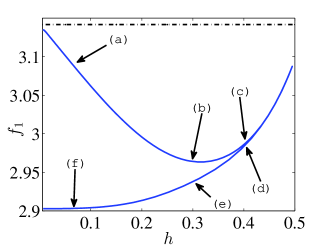
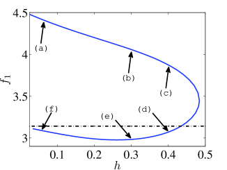
Figure 1: Plot of the static discrete profiles evaluated at the first site of the domain as functions of lattice spacing $h$, i.e., $f_{1}(h)$, for $\alpha=4$ (left panel) and $\alpha=5$ (right panel). The value of $\pi$ appears in both figures as a dashed-dotted black line.

In this section, the existence, time evolution as well as (a suitably tailored variant of) stability of static discrete BPS skyrmions are studied when the free parameter $\alpha$ takes the values: $\alpha=4$ and $\alpha=5$. In particular, a Newton-Krylov method [6] has been employed together with a suitable initial guess in order to ensure convergence towards a steady-state solution (i.e., a stationary BPS skyrmion on the lattice) of equations (9). As a starting point (developing the continuum limit solution), the BPS equation (5) with the minus sign was solved numerically using a spline collocation method [7]. Then, the obtained profile function $f(r)$ was fed to the Newton solver in order to identify steady states of the lattice equations (9) within $10^{-10}$ (user-prescribed) tolerance. Finally, a pseudo-arclength continuation over the lattice spacing $h$ was performed by utilizing the bifurcation software AUTO [8].

For instance, for the cases with $\alpha=4$ and $\alpha=5$, Figure 1 showcases the functional dependence of $f_{1}$, i.e., the value of the profile function at the first site in the domain, over the lattice spacing $h$ in the left and right panels, respectively. Furthermore, typical sample examples of static lattice BPS skyrmions, i.e., plots of $f_{m}\doteq f(mh)$ against $m$, are shown in Figures 2 and 3 for various values of $h$ (see the captions in the relevant figures in connection with the arrows appearing in Figure 1).

These solutions provide a sense of the variation of the solution over the branch. In Figure 2 (case of $\alpha=4$), the profile (a) is the most proximal to the continuum limit, panels (b) and (c) arise in progressively more discrete settings, while the ones of (d)-(f) give relevant examples of the same solution branch past the fold point. A similar phenomenology can be found in Figure 3 (case of $\alpha=5$), although now (f) represents the solution most proximal to the continuum one. It is additionally intriguing that a number of the solutions appear to have a “concave down” profile as they tend to zero: that is shown in panels (a) and (f), suggesting a nearly compact waveform in the relevant solutions. In each case of $\alpha$, one of the branches seems to be more “coarse” and more discrete in nature, while the other is more proximal to the continuum limit.

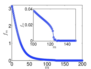
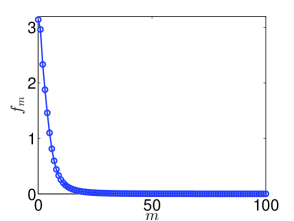
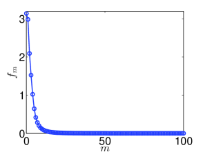
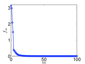
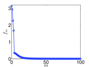
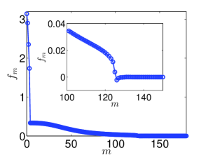
Figure 2: Static discrete profiles corresponding to the $\alpha=4$ branch (see, the left panel of Figure 1) for $h=0.06$: panels (a) and (f); $h=0.3$: panels (b) and (e); and $h=0.4$: panels (c) and (d).

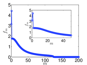
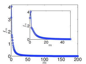
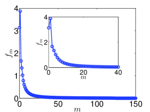
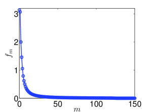
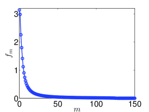
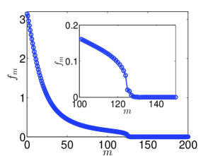
Figure 3: Same as Figure 2 for $\alpha=5$ branch (see, the right panel of Figure 1). In particular, static discrete profiles for $h=0.06$: panels (a) and (f); $h=0.3$: panels (b) and (e); and $h=0.4$: panels (c) and (d).

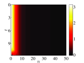
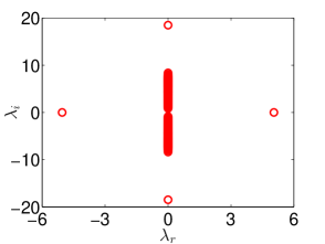
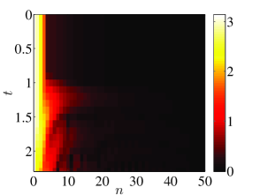
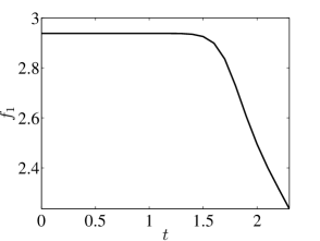
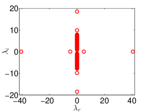
Figure 4: Spatio-temporal evolution of the steady-state solutions of panels (b) and (e) of Figure 2 and associated spectra for $\alpha=4$ and $h=0.3$ are shown at the top and bottom panels, respectively. The left and middle panels correspond to the space-time evolution of the profile function and the dependence of $f_{1}$ on time $t$, respectively, whereas the right panels present the corresponding spectra.

Next, we study the dynamics of the BPS skyrmions for $h=0.3$ and $h=0.4$ while $\alpha=4$ and $\alpha=5$ and investigate their stability. It is now of crucial importance to highlight that the time-dependent ODEs (9) require careful handling from the numerical computations’ point of view. Specifically, the second order in-time system involves a denominator of the form of $\sin^{4}(\frac{f_{+}+f}{2})$ which for large $m$, i.e., far from the origin, becomes zero due to the fact that the discrete profiles asymptote to zero. This leads to significant complications in the numerical computations, and a special treatment of such terms is needed, in order to avoid overflow in the computations. To overcome this issue, we impose an artificial cut-off to the discrete profiles, that is, we truncate the computational domain from the original into a new one such that the value of the profile function at the next-to-last site is of the order of $10^{-4}$. For consistency, the same homogeneous boundary condition is employed and the “new”, free-from-overflow profile is again a solution to the steady version of equations (9). In this way, a stability analysis can be carried out for such steady-state profiles as follows. The perturbation ansatz of the form of

$$f=f^{0}+\varepsilon\,e^{\lambda t}w,\quad(\varepsilon\ll 1),$$ (10)

is introduced with $f^{0}$ being a steady state, $w\doteq w(mh)$, and at order $\varepsilon$, Eq. (9) results in an eigenvalue problem with $\left(\lambda,w\right)$ representing the corresponding eigenvalue and eigenvector, respectively. If any of the eigenvalues $\lambda=\lambda_{r}+i\lambda_{i}$ has a positive real part, the underlying steady state is deemed to be unstable (on the other hand, marginal stability arises only when all the eigenvalues are found to be imaginary, i.e., correspond to small oscillations around the equilibrium). Results for the dynamics of BPS skyrmions for $\alpha=4$ and $\alpha=5$ with $\dot{f}_{m}=0$ ($m>1$, i.e., in the absence of initial speed) as well as associated spectra are shown in Figures 4 and 5; 6 and 7, respectively. These case examples are performed for the points (b), (e) and (c), (d) in each branch (and for both $\alpha=4$ and $\alpha=5$) i.e., for the cases where discreteness plays a more pronounced role in the results.

It can be discerned from the Figures 4-7 that the BPS skyrmions are generally deemed to be unstable and this is also confirmed by computing the associated spectra of the solutions (see, the right panels therein). These instabilities are either manifested via a drastic (localized) amplitude decay as in Figures 4(a)-(b) and Figures 6(c)-(d); or through the emission of radiative wavepackets as in Figures 4(c)-(d) and Figures 5(c)-(d). They may also lead to oscillatory dynamics such as those observed in Figures 5(a)-(b) and Figures 7(c)-(d). However, it is important to note that in the case of $\alpha=5$ (Figures 6 and 7) for $h=0.3$ and $h=0.4$ (depicted in panels (b) of the respective figures), the discrete BPS skyrmions appear to be long-lived ones over a wide time window (see the range of the $x$-axis). This is also corroborated by our linear stability analysis results for these particular cases since all the eigenvalues $\lambda$ are sitting on the imaginary axis, thus suggesting that the pertaining waveforms are (indeed) stable. Hence, these solutions are promising for a discrete realization of BPS skyrmionic structures.

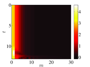
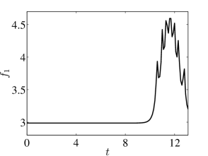
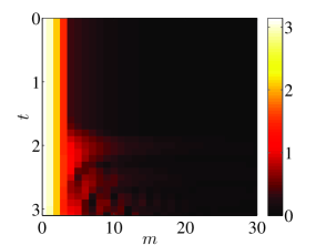
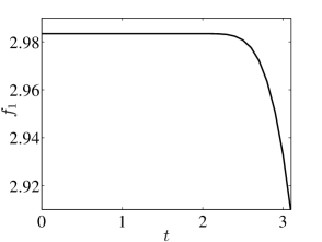
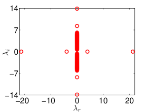
Figure 5: Same as Fig. 4 but for $h=0.4$. Spatiotemporal evolution of the steady-state solutions of panels (c) and (d) of Figure 2 and associated spectra are shown at the top and bottom panels, respectively. The left and middle panels correspond to the space-time evolution of the profile function and the dependence of $f_{1}$ on time $t$, respectively, whereas the right panels present the underlying spectra.

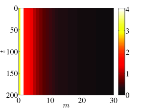
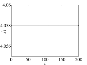
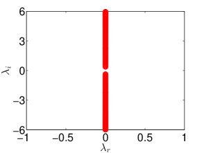
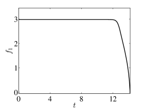
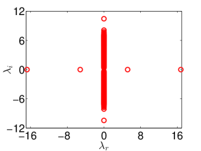
Figure 6: Same as Fig. 4 but for $\alpha=5$ and $h=0.3$. Spatio-temporal evolution of the steady-state solutions of panels (b) and (e) of Figure 3 and associated spectra are shown at the top and bottom panels, respectively. Left, middle and right panels are the same as in the previous figures.

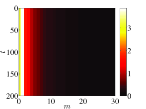
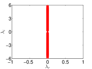
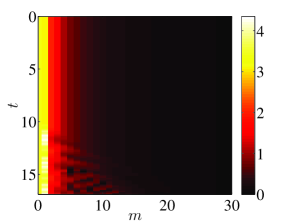
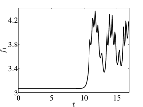
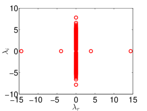
Figure 7: Same as Fig. 6 but for $h=0.4$. Spatiotemporal evolution of the steady-state solutions of panels (c) and (d) of Figure 3 and associated spectra are shown at the top and bottom panels, respectively. Again, the left, middle and right panels are the same as before.

5 Conclusions and Future Challenges

In the present work, we have revisited the topic of discrete skyrmions in the context of the so-called BPS model. We have provided a discretization motivated by the enforcement of the Bogomolny bound of the model. This results in a Hamiltonian model that is, however, highly nonlinear in that the kinetic energy term is multiplied by a sinusoidal function of the field. We have discussed the numerous nontrivial complications/challenges that such a feature presents from a numerical perspective, as well as a possible way to overcome them. On the one hand, it is not possible at the present stage to conduct a systematic spectral stability analysis of these solutions at least in the form involving their vanishing tails (given the relevant small denominators that arise in the eigenvalue computation). A similar problem renders rather difficult the examination of the dynamical evolution of the solutions. Nevertheless, utilizing a suitable truncation, we have not only been able to monitor the waveforms in direct numerical simulations, but also to corroborate our findings in the realm of linear stability analysis in the cases reported in this work. Our results have revealed that the identified solutions are typically unstable. However, for larger values of the potential parameter $\alpha$, it is possible to find long-lived case examples of the relevant states, which are promising candidates for discrete BPS skyrmions.

Naturally, there are numerous open questions that emerge from this study. One such involves the fact that the higher values of $\alpha$ considered here appear to have a better chance to lead to long-lived states. Hence, it would be interesting to find out if for sufficiently large $\alpha$’s the solution becomes generically (potentially) robust. Another question is that of the spectral stability: is it possible (perhaps via tricks like the one of domain truncation utilized here) to obtain meaningful information about the spectral stability of these solutions? In the present work, we have partially answered this question, although it would be useful to explore that systematically for the branches presented herein. Finally, here we have studied the radial problem for the BPS Skyrme model case. It would be relevant to explore the effect of azimuthal perturbations and the nature of their impact on the stability and dynamics of the considered discrete skyrmion states. Such studies will be considered in future publications.

6 Acknowledgments

M.A acknowledges support from FP7, Marie Curie Actions, People, International Research Staff Exchange Scheme (IRSES-606096). T.I. acknowledges support from FP7, Marie Curie Actions, People, International Research Staff Exchange Scheme (IRSES-606096); and from The Hellenic Ministry of Education: Education and Lifelong Learning Affairs, and European Social Fund: NSRF 2007-2013, Aristeia (Excellence) II (TS-3647).

References

- [1] T.H.R. Skyrme, Proc. Roy. Soc. London A. 260 (1961) 127-138; 262 (1961) 237-245; Nucl. Phys. 31 (1962) 556-569.
- [2] C. Adam, J. Sanchez-Guillen, and A. Wereszczynski, Phys. Lett. B 691 (2010) 105; Phys. Rev. D 82 (2010) 085015; C. Adam, C. Naya, J. Sanchez-Guillen, and A. Wereszczynski, Phys. Rev. Lett. 111 (2013) 232501; C. Adam, C.D. Fosco, J.M. Queiruga, J. Sanchez-Guillen, and A. Wereszczynski, J. Phys. A: Math. Theor. 46 (2013) 135401.
- [3] T. Ioannidou and A Lukacs, J. Math. Phys. 57 (2016) 022901.
- [4] E. Charalampidis, T. Ioannidou and P. Kevrekidis, Phys. Scripta 90 (2015) 2, 025202.
- [5] C. Houghton, N. Manton and P. Sutcliffe, Nucl. Phys. B 510 (1998) 587; T. Ioannidou, B. Piette and W. J. Zakrzewski, J. Math. Phys. 40 (1999) 6353; J. Math. Phys. 40 (1999) 6223.
- [6] C. T. Kelley, Solving Nonlinear Equations with Newton’s Method (Fundamentals of Algorithms, SIAM, Philadelphia, 2003).
- [7] U. Ascher, J. Christiansen and R.D. Russell, Math. Comput. 33 (1979) 659; ACM Trans. Math. Softw. 7 (1981) 209.
- [8] E. Doedel, AUTO, indy.cs.concordia.ca/auto/.