Prior Variances and Depth Un-Biased Estimators in EEG Focal Source Imaging

Abstract

In electroencephalography (EEG) source imaging, the inverse source estimates are depth biased in such a way that their maxima are often close to the sensors. This depth bias can be quantified by inspecting the statistics (mean and covariance) of these estimates. In this paper, we find weighting factors within a Bayesian framework for the used $\ell_{1}/\ell_{2}$ sparsity prior that the resulting maximum a posterior (MAP) estimates do not favour any particular source location. Due to the lack of an analytical expression for the MAP estimate when this sparsity prior is used, we solve the weights indirectly. First, we calculate the Gaussian prior variances that lead to depth un-biased maximum a posterior (MAP) estimates. Subsequently, we approximate the corresponding weight factors in the sparsity prior based on the solved Gaussian prior variances. Finally, we reconstruct focal source configurations using the sparsity prior with the proposed weights and two other commonly used choices of weights that can be found in literature.

1 Introduction

In EEG focal source imaging, the goal is to estimate the focal neural activity that arises, for example, during an epileptic seizure using scalp potentials. Based on the distributed source modelling [1], the mapping that connects the dipole moments of $n$ potential source locations to $m$ scalp-potential measurements can be written as

$$v=Kd+\xi,$$ (1)

where $v\in\mathbb{R}^{m}$, $K\in\mathbb{R}^{m\times kn}$ ($m\ll kn$) is the lead field matrix, $k$ is the dimension of the problem (2D or 3D), $d\in\mathbb{R}^{kn}$ is the distributed dipole source configuration and $\xi\sim\mathcal{N}(0,\Gamma_{\xi})$ is the measurement noise.

The ill-posedness of the associated inverse problem requires the use of prior information to obtain stable estimates. One way to solve the problem is to find the estimate of the under-determined linear system that has the minimum norm [2]. However, the minimum norm estimate (MNE) has the property that its maxima can lie only close to the sensors, because the measured scalp potentials can be generated from superficial source configurations with less power than from deep source configurations [3]. Similar source reconstructions can also be obtained with $\ell_{2}$-norm priors. Even if $\ell_{1}$-norm priors are employed the solution consists of several scattered superficial sources [4].

To reduce the depth bias several (often heuristic) approaches have been suggested [5, 6, 3, 7, 8]. The most common approaches are to weight all the sources in the penalty term with the norm of the corresponding column of the lead field matrix [5, 9] or the diagonal elements of the model resolution matrix [10, 11]. Another approach is to use the Bayesian hierarchical modelling [12].

In this paper, our aim is to find, within a Bayesian framework, weights for our sparsity prior such that the resulting posterior estimates do not favor any particular source location or component. Because there is no analytical expression for the MAP estimate when sparsity priors are employed, we propose to solve the weights indirectly. We first quantify the depth bias of the maximum a posterior (MAP) estimates when an i.i.d. Gaussian prior is employed by inspecting the statistics of the MAP estimates. Next, we calculate the Gaussian prior variances that ensure depth un-biased solutions by equalizing the variances in the covariance matrix of the MAP estimates. Finally, we approximate the corresponding weighting factors in the sparsity prior using the solved Gaussian prior variances. We demonstrate the feasibility of our approach by simulating focal brain activity with finite element (FE) simulations. In the reconstructions, we employ the weighted $\ell_{1}/\ell_{2}$ sparsity prior and we compare the results obtained using our proposed weights with the reconstructions based on two other commonly used choices of depth weights.

2 Theory

2.1 Bayesian Inversion

In the Bayesian framework, the inverse solution is the posterior density of the Bayes formula

$$\pi(d|v)\propto\pi(v|d)\pi(d),$$ (2)

where $\pi(v|d)$ is the likelihood and $\pi(d)$ the prior. From Equation (1), the likelihood is

$$\pi(v|d)\propto\exp\Big{(}-\frac{1}{2}(v-Kd)^{\mathrm{T}}\Gamma_{\xi}^{-1}(v-Kd)\Big{)}.$$ (3)

The MAP estimate of the reconstructions is [13],

$$\hat{d}:=\min_{d\;\in\;\mathbb{R}^{kn}}\|L_{\xi}(Kd-v)\|_{2}^{2}-2\ln\pi(d),$$ (4)

where $L_{\xi}$ comes from the Cholesky factorization of $\Gamma_{\xi}$.

2.2 Gaussian prior

Let us consider a Gaussian prior

$$\pi(d)\propto\exp{\left(-\frac{1}{2}d^{\mathrm{T}}\Gamma_{d}^{-1}d\right)}$$ (5)

that does not have depth weights i.e. the covariance matrix is $\Gamma_{d}=\alpha^{-2}I$ where $I$ is the identity matrix and $\alpha^{2}$ a scaling parameter. In this case, the MAP estimate is [2]

$$\hat{d}=K^{\mathrm{T}}(KK^{\mathrm{T}}+\alpha^{2}\Gamma_{\xi})^{-1}v.$$ (6)

From variational point of view, this MAP estimate coincides with Tikhonov regularization and thus yields to a harmonic solution that attains its maximum at the boundary [4]. This can also be explained statistically by analyzing the expectation value and covariance of the MAP estimates. Theses values can be estimated by sampling or by using the analytical expressions

$$\mathbb{E}[\hat{d}]=0\;\;\;\mbox{ and }\;\;\;\Gamma_{\hat{d}}=\mathbb{E}[\hat{d}\hat{d}^{\mathrm{T}}]=K^{\mathrm{T}}(KK^{\mathrm{T}}+\alpha^{2}\Gamma_{\xi})^{-1}K.$$ (7)

Figure 1-A shows how the values of the diagonal elements (variances) of $\Gamma_{\hat{d}}$ decrease almost quadratically with respect to depth. The zero expectation values and the very low variances associated with the deep locations imply that the deep sources are very unlikely to be reconstructed. Thus, this MAP estimator is biased with respect to depth and favors sources close to the sensors.

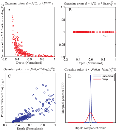
Figure 1: A and B: The diagonal elements of $\Gamma_{\hat{d}}$ with respect to depth when the i.i.d. and depth compensated Gaussian prior are used, respectively. C: The posterior variances w. r. t. depth when the depth compensated prior is used. D: Two marginal distributions of the posterior.

In this paper, our aim is to determine such prior variances that the resulting MAP estimates do not favor any particular source location or component over other i.e. the variances of the MAP estimates are equal.

We start by postulating that this prior covariance matrix is diagonal $\Gamma_{d}=\alpha^{-2}\mathrm{diag}(\gamma_{d}^{(i)})$ for $i=1,\ldots,kn$. The MAP estimate corresponding to this prior is

$$\hat{d}=\Gamma_{d}K^{\mathrm{T}}(K\Gamma_{d}K^{\mathrm{T}}+\alpha^{2}\Gamma_{\xi})^{-1}v,$$ (8)

and the covariance of the MAP estimates becomes

$$\Gamma_{\hat{d}}=\mathbb{E}[\hat{d}\hat{d}^{\mathrm{T}}]=\Gamma_{d}K^{\mathrm{T}}(K\Gamma_{d}K^{\mathrm{T}}+\Gamma_{\xi})^{-1}K\Gamma_{d}.$$ (9)

In a similar way as in [14], we estimate the prior variances by minimizing

$$\gamma_{d}:=\min_{\gamma_{d}}\|\mathrm{diag}(\alpha^{-2}I-\Gamma_{\hat{d}})\|_{2}^{2}.$$ (10)

This results in solving a set of non-linear equations

$$\alpha^{2}=\gamma_{d}^{2(i)}{K}^{(:,i)\mathrm{T}}M{K}^{(:,i)}\;\;\;\;\;\mbox{ for }i=1,\ldots,kn,$$ (11)

where $M=(\Gamma_{{\xi}}+K\Gamma_{{d}}K^{\mathrm{T}})^{-1}$ and ${K}^{(:,i)}$ is the $i^{th}$ column.

Figure 1-B shows that with these prior variances the diagonal elements of $\Gamma_{\hat{d}}$ will be equal, or in other words, the corresponding MAP estimator is depth unbiased. Moreover, Figure 1-C depicts the diagonal elements of the posterior covariance $\Gamma_{d|v}=(K^{\mathrm{T}}\Gamma_{\xi}^{-1}K+\Gamma_{d}^{-1})^{-1}$ obtained based on the estimated prior and Figure 1-D shows two corresponding marginal posterior densities of two different locations. We can observe that the posterior dipole variances increase with respect to depth. Qualitatively, this means that in the estimated source configurations the deep sources are allowed to have higher strengths than the superficial sources, and therefore, the solutions can attain their maximum also deeper in the brain (and not only close to the sensors).

2.3 $\ell_{1}/\ell_{2}$- norm sparsity prior

In this paper, we consider sparse focal source reconstructions and therefore, we employ the $\ell 1/\ell_{2}$-norm prior

$$\pi(d)\propto\exp{\left({-\frac{\alpha}{2}\sum_{i=1}^{n}w^{r}_{i}\|\mathrm{d}_{i}\|_{2}}\right)}$$ (12)

where $d_{i}=(d_{ix},d_{iy},d_{iz})$, $\|d_{i}\|_{2}=\sqrt{d_{ix}^{2}+d_{iy}^{2}+d_{iz}^{2}}$ is the strength of the source at location $i$ and $w_{i}^{r}$ are the weights. For short, we denote the dipole strength at location $i$ as ${r}_{i}=\|\mathrm{d}_{i}\|_{2}$ and

$$\pi(r_{i})\propto\exp{\left(-\frac{\alpha}{2}w^{r}_{i}r_{i}\right)}.$$ (13)

The variance of $\pi(r_{i})$ is

$$\gamma_{r}^{(i)}=c\int_{0}^{\infty}(r_{i}-r_{*i})^{2}\exp{\left(-\frac{\alpha}{2}w_{i}^{r}r_{i}\right)}~{}dr_{i}=\frac{4}{\alpha^{2}{(w^{r}_{i})}^{2}}$$ (14)

where $r_{*i}=c\int_{0}^{\infty}r_{i}\exp{\left(-0.5\alpha w_{i}^{r}r_{i}\right)}~{}dr_{i}=\frac{4c}{\alpha^{2}{(w_{i}^{r})}^{2}}$ and $c=0.5\alpha w_{i}^{r}$ because $\int_{0}^{\infty}c\exp{\left(-0.5\alpha w_{i}^{r}r_{i}\right)}~{}dr_{i}=1$.

We calculate $\gamma_{r}^{(i)}$ at location $i$ with the help of the corresponding Gaussian variances $\gamma_{d}^{(i+(j-1)n)}$ as

$$\gamma_{r}^{(i)}=k\alpha^{-2k+2}\left(\prod\limits^{k}_{j=1}\gamma_{d}^{(i+(j-1)n)}\right)\left(\sum\limits^{k}_{j=1}\gamma_{d}^{(i+(j-1)n)}\right)^{-1},$$ (15)

where $j=1,\ldots,k$ and $k$ is the dimension of the problem. This choice ensures that $\gamma_{r}^{(i)}$ is roughly the average of the dipole component variances when the variances of the components are similar and that $\gamma_{r}^{(i)}$ is close to the lowest dipole component variance when the variances have large differences. Finally, from Equation (14) and (15) we calculate the weights

$$w_{i}^{r}=2\sqrt{\frac{\alpha^{2k-4}}{k}\frac{\sum\limits_{j=1}^{k}\gamma_{d}^{(i+(j-1)n)}}{2\prod\limits_{j=1}^{k}\gamma_{d}^{(i+(j-1)n)}}}$$ (16)

The estimated Gaussian variances and the corresponding weights of the $\ell_{1}/\ell_{2}$-norm prior are shown in Figure 2.

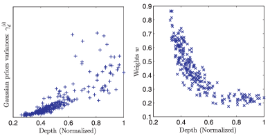
Figure 2: The estimated Gaussian prior variances $\gamma_{d}^{(i)}$ and the corresponding weights for the $\ell_{1}/\ell_{2}$ norm prior with respect to depth .

3 Materials and methods

We study the proposed weights by simulating focal deep sources in the gray matter of a 2D FE head model. The head model consisted of five compartments with conductivities (in S/m) equal to $0.33$ for the scalp, $0.015$ for the skull, $1.76/0.016/0.33$ for the cerebral spinal fluid, gray matter and white matter [15], respectively. The potential measurements $v$ were obtained from 32 point sensors equally spaced around the boundary. For the forward and the inverse computations, we use two meshes with 2342 and 1236 nodes, respectively.

The MAP estimate of the dipole configuration with sparsity constraint is

$$\hat{d}_{\mathrm{MAP}}:=\min_{d}\|v-Kd\|_{2}^{2}+\sum_{i=1}^{n}\lambda w_{i}\|\mathrm{d}_{i}\|_{2}w$$ (17)

where $\lambda$ is a tuning parameter. The minimization is performed by using the interior point method [16] with Bregman iterations [17]. The performance of the proposed weights, $w_{i}^{r}$, from Equation (16), was compared with two other commonly used weights: first, the MNE resolution weights given by $w_{i}^{\mathrm{MNE}}=\sqrt{1/k\sum_{j=1}^{k}R^{(i,i+(j-1)n)}}$, where $R^{(i,i)}=\mathrm{diag}(K^{\mathrm{T}}(KK^{\mathrm{T}}+\Gamma_{\xi})^{-1}K)$ [11] and second, the normalized maximum sensor responses $w^{\mathrm{M}SR}_{i}=g_{i}/\max{(g_{i})}$, where $g_{i}=\max_{l=1:m}\left(\|1/k\sum_{j=1}^{k}K^{(l,i+(j-1)n)}\|_{2}\right)$ [18]. To access the ground truth, we consider measurements with high signal to noise ratio, $\mathrm{SNR}=60$dB. For the quantitative comparison of the results we employ the earth mover’s distance (EMD) [19].

4 Results and discussion

We demonstrate the performance of the different weights using three test cases with one and two dipole sources. In Figure 3, the small images on the left hand side show the true dipoles, the location is marked with blue circles and the orientations with small blue lines. The remaining images, starting from left, show the reconstruction when $w_{i}^{\mathrm{MNE}}$, $w_{i}^{\mathrm{MSR}}$ and $w_{i}^{r}$ are used as weights, respectively. The blue marker $\mathrm{x}$ shows the locations of true sources. The MAP estimates were computed by solving Equation (17).

All the tested weights give feasible reconstructions. However, we note that the proposed weights $w_{i}^{r}$ give the least scattered results and work the best in the single focal source cases. For the two source case, all the weights give roughly similar reconstructions and EMD values.

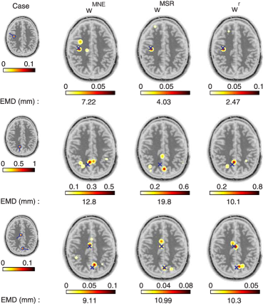
Figure 3: Reconstructed source distributions using different weights in the $\ell_{1}/\ell_{2}$ prior model. The images show first the test cases and then the reconstructions with the different weights $w_{i}^{\mathrm{MNE}}$, $w_{i}^{\mathrm{MSR}}$ and $w_{i}^{r}$, respectively.

5 Conclusion and future work

We have demonstrated that the proposed depth weights with the $\ell_{1}/\ell_{2}$ sparsity prior give better reconstruction compared to two commonly used weights when single deep sources are studied. Our proposed approach has the benefit that it does not require using hyper-parameter models that would involve extensive sampling due to the lack of an analytical expression for the MAP estimate when the $\ell_{1}/\ell_{2}$ prior is used. In the future, Monte Carlo simulations will be carried out in a 3D head model to analyze the distribution of the MAP estimates reconstructed by using the $\ell_{1}/\ell_{2}$ sparsity prior with the proposed weights.

Conflict of interest

The authors declare that they have no conflict of interest.

	Corresponding author: Alexandra Koulouri
	Institute: University of Münster
	Street: Einsteinstrasse 62
	City: Münster
	Country: Germany
	Email: koulouri@uni-muenster.de

References

- [1] Baillet S., Mosher J. C., Leahy R. M. Electromagnetic brain mapping IEEE Signal Processing Magazine. 2001;18:14–30.
- [2] Hämäläinen M. S., Ilmoniemi R. J. Interpreting magnetic fields of the brain: minimum norm estimates Med. & Biol. Eng. and Com. 1994;32:35–42.
- [3] Fuchs M., Wagner M., Wischmann H.-A. Linear and Nonlinear Current Density Reconstructions Journal of Clinical Neurophysiology. 1999;16:267–295.
- [4] Burger M., Dirks H., Müller J. Inverse Problems in Imaging. Rad. Ser. Comp. App. 2013.
- [5] Köhler T., Wagner M., Fuchs M., Wischmann H. A., Drenckhahn R., Theissen A. Depth normalization in MEG/EEG current density imaging in Proc. of 18th An. Int. Conf. of the IEEE Eng. in Med. and Biol. Soc.;2:812-813 vol.2 1996.
- [6] Pascual-Marqui R. D., Michel C. M., Lehmann D.. Low resolution electromagnetic tomography: a new method for localizing electrical activity in the brain Int. J. Psychophysiol.. 1994;18:49–65.
- [7] Wagner M., Wischmann H.-A., Fuchs M., Köhler T., Drenckhahn R. Current Density Reconstructions Using the L1 Norm:393–396. Springer New York 2000.
- [8] Palmero-Soler E., Dolan K., Hadamschek V., Tass P.A. swLORETA: a novel approach to robust source localization and synchronization tomography Phys. in Med. and Biol.. 2007;52:1783–1800.
- [9] Lin F.-H., Belliveau J. W., Dale A. M., Hämäläinen M. S. Distributed current estimates using cortical orientation constraints Human Brain Mapping. 2006;27:1–13.
- [10] Pascual-Marqui R. D. Standardized low resolution brain electromagnetic tomography (sLORETA): technical report Meth. and finding in exprerim. and clin. pharm. 2002;24 Suppl, D:5-12.
- [11] Haufe S., Nikulin V. V., Ziehe A., Müller K.-R., Nolte G. Combining sparsity and rotational invariance in EEG/MEG source reconstruction. NeuroImage. 2008;42:726-738.
- [12] Lucka F., Pursiainen S., Burger M., Wolters C. H. Hierarchical Bayesian inference for the EEG inverse problem using realistic FE head models: Depth localization and source separation for focal primary currents NeuroImage. 2012;61:1364–1382.
- [13] Kaipio J. P., Somersalo E. Statistical and Computational Inverse Problems;160 of Applied Mathematical Series. Springer-Verlag New York1 ed. 2005.
- [14] Pascual-Marqui R. D.. Discrete, 3D distributed, linear imaging methods of electric neuronal activity. Part 1: exact, zero error localization arXiv:0710.3341[math-ph]. 2007.
- [15] Vorwerk J., Cho J.-H., Rampp S., Hamer H., Knösche T. R., Wolters C. H. A guideline for head volume conductor modeling in EEG and MEG NeuroImage. 2014;100:590-607.
- [16] Boyd S. P., Vandenberghe L. Convex Optimization. Cambridge University Press 2004.
- [17] Yin W., Osher S., Goldfarb D., Darbon J. Bregman iterative algorithms for l1-minimization with applications to compressed sensing SIAM J. Imaging Sci. 2008:143–168.
- [18] M. Fuchs, M. Wagner, A. Wischmann H. Generalized minimum norm least squares reconstruction algorithms in ISBET Newsletter (ISSN 0947-5133)no. 5:8–11 1994.
- [19] Rubner Y., Tomasi C., Guibas L. J. The Earth Mover’s Distance as a Metric for Image Retrieval Int. J. of Comp. Vision. 2000;40:99–121.