Optimization of Vehicle Connections in V2V-based Cooperative Localization

Abstract

Cooperative map matching (CMM) uses the Global Navigation Satellite System (GNSS) positioning of a group of vehicles to improve the standalone localization accuracy. It has been shown to reduce GNSS error from several meters to sub-meter level by matching the biased GNSS positioning of four vehicles to a digital map with road constraints in our previous work. While further error reduction is expected by increasing the number of participating vehicles, fundamental questions on how the vehicle membership of the CMM affects the performance of the GNSS-based localization results need to be addressed to provide guidelines for design and optimization of the vehicle network. The quantitative relationship between the estimation error and the road constraints has to be systematically investigated to provide insights. In this work, a theoretical study is presented that aims at developing a framework for quantitatively evaluating effects of the road constraints on the CMM accuracy and for eventual optimization of the CMM network. More specifically, a closed-form expression of the CMM error in terms of the road angles and GNSS error is first derived based on a simple CMM rule. Then a Branch and Bound algorithm and a Cross Entropy method are developed to minimize this error by selecting the optimal group of vehicles under two different assumptions about the GNSS error variance.

I INTRODUCTION

Low-cost Global Navigation Satellite Systems (GNSS) are used for most mobile applications, with localization error of several meters. The limited accuracy of the low-cost GNSS is mainly due to the atmospheric error, referred to as the common error, as well as receiver noise and multipath error, referred to as the non-common error. Various techniques have been used to reduce GNSS localization error such as precise point positioning (PPP) [1], real time kinematics (RTK) [2] and sensor fusion [3]. Nonetheless, improving the localization accuracy of the widespread GNSS without incurring additional hardware and infrastructure costs has motivated recent research activities on cooperative GNSS localization [4] and cooperative map matching (CMM) [5], [6], [7].
CMM improves the GNSS localization accuracy by matching the GNSS positioning of a group of connected vehicles to a digital map. With the reasonable assumption that vehicles should travel on the roads, the road constraints can be applied to correct the GNSS positioning. CMM is much more powerful in exploiting the road constraints than ego-localization with map matching.

Figure 1: Illustration of the positioning correction through CMM

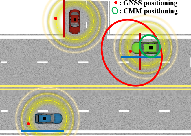
Fig. 1 illustrates how error-corrupted GNSS information is corrected through a naive CMM approach. The GNSS solutions, denoted as red dots, of all the three vehicles are biased away from their true positions, while the biases are highly correlated. Virtual constraints from the red and the blue vehicle are applied to restrict the positioning of the green vehicle. The underlying assumption for the application of the virtual constraints is that the GNSS positioning biases of the three vehicles are the same. This example manifests the effect of road constraints on the CMM localization.
The limited bandwidth of the Dedicated Short Range Communication (DSRC)-based connected vehicle network imposes an upper limit on the maximal number of connected vehicles to avoid frequent package loss [8], but typically the number of vehicles within the communication range is more than the upper limit. This limitation motivates the development of an optimization scheme that selects $M$ vehicles with optimal road constraints that minimizes CMM localization error, where $M$ is the maximal number of connected vehicles. To achieve this goal, it is necessary to quantify the effect of road constraints on the CMM localization error. This is, nevertheless, not easily achievable as the algorithms that implement CMM are usually sophisticated, and there is no analytic expression relating the localization error with the road constraints for these algorithms.
Recently, two different CMM algorithms have been developed for GNSS common error estimation problem, i.e., a non-Bayesian particle-based approach in Rohani et. al. [5] and a Bayesian approach based on a Rao-Blackwellized Particle Filter in our previous work [6], [7]. One common feature of these two CMM algorithms is that the probabilistic property of the GNSS error is utilized. This increases the localization accuracy and robustness, but also leads to complicated mapping between the localization error and the road constraints, which makes the analysis of the effects of road constraints rather difficult.
In our previous work [9], the correlation between the localization error and the road constraints is quantified analytically. More specifically, a closed-form expression of the estimated localization error in terms of the road angles as well as the GNSS error is derived based on a simple CMM rule that neglects the probabilistic property of the GNSS error as well as historical GNSS measurements. As a result of these simplifications, this closed-form expression is not sufficient to accurately predict the localization error of the particle filter based CMM algorithm. Nonetheless, it can be used to select the optimal set of connected vehicles, on which the CMM error is expected to be minimized with the particle filter based CMM algorithm. In this work, two algorithms are developed to optimize the connected vehicle selection such that the closed-form expression of the estimated localization error is minimized. These results provide a guideline for the implementation of CMM.
In the following sections, details about the derivation of the CMM localization error and the optimization algorithms are presented. In Section 2, the notions in CMM are introduced. Then a simple CMM rule is applied to derive an analytic expression of the localization error. Based on this error formula, in Section 3, two algorithms are presented to minimize the localization error through the optimal selection of connected vehicles. A Branch and Bound (B&B) [10] searching algorithm is developed in the case that all the vehicles have the same non-common GNSS error variance. A Cross Entropy (CE) method [11] combined with a heuristic pre-selection step is developed in the case that vehicles have different non-common GNSS error variances. In Section 4, the contributions and conclusions are summarized.

II CMM localization error

In this section, we propose a framework of vehicle positioning within a reference road framework to facilitate the analytic investigation.
The following assumptions are essential in the derivation:

1. The GNSS common error is the same for all the connected vehicles within the vehicular network.

2. The road side can be locally approximated as a straight line.

3. The GNSS non-common error is small enough such that the exact expression for the estimation error can be approximated by its first order linearization with respect to the non-common error.

4. The GNSS non-common error is a random variable that obeys the Gaussian distribution.
   

The first assumption is reasonably accurate as long as the connected vehicles are geographically close to each other, for example, within several miles. The second and the third assumptions are made for mathematical convenience. If they are violated, however, the exact expression of the estimation error will still be valid but the asymptotic approximation will be inaccurate. The last assumption has been experimentally verified in [6] under open sky conditions.

Figure 2: Illustration of the notations used in CMM

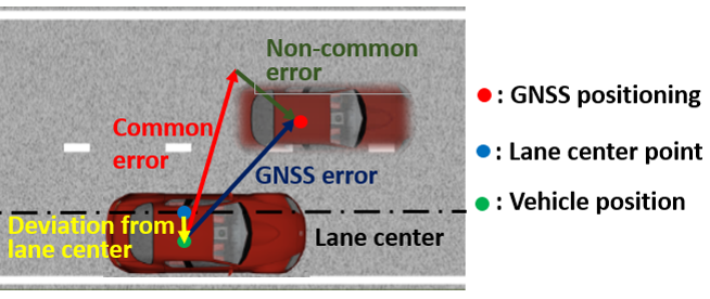
Consider a network of connected vehicles, the coordinate of GNSS positioning of the $i$-th vehicle can be decomposed into a superposition of the coordinate of a point on the corresponding lane center, the deviation of the vehicle from the lane center, the common error and the non-common error as illustrated in Fig. 2. The grayscale image of the vehicle represents the GNSS positioning. This decomposition can be expressed mathematically as

$$x^{G}_{i}=x^{L}_{i}+x^{D}_{i}+x^{C}+x^{N}_{i},i=1,2,...,N,$$ (1)

where $x^{G}_{i}$ is the GNSS positioning of the $i$-th vehicle, $x^{L}_{i}$ is the closest point on the center of the lane from the vehicle, $x^{D}_{i}$ is the deviation of the vehicle coordinates from $x^{L}_{i}$, $x^{C}$ is the GNSS common error, $x^{N}_{i}$ is the GNSS non-common error.
The fact that all the vehicles travel on the roads can be expressed as a set of inequalities

$$g_{i}(x^{G}_{i}-x^{C}-x^{N}_{i})<0.$$ (2)

Applying the second assumption, the constraint functions $g_{i}$ have simple analytic forms

$$g_{i}(x)=(x-x^{L}_{i})\cdot n_{i}-w,$$ (3)

where $\{\cdot\}$ is the dot product operator, $n_{i}$ is the unit vector normal to the lane center point towards outside of the road and $w$ is the half width of the lane.
Eq. (2) can be interpreted as the feasible set of the common error given the GNSS positioning and the non-common error. The non-common error is unknown, however, to the implementation of CMM. Thus, the following approximation of the feasible set by neglecting the non-common error is used instead of the exact feasible set,

$$\Omega =\{\tau|\bigcap\limits_{i=1}^{N}g_{i}(x^{G}_{i}-\tau)<0\}$$ (4)

$$=\{\tau|\bigcap\limits_{i=1}^{N}g_{i}(x^{L}_{i}+x^{C}+\tilde{x}^{N}_{i}-\tau)<0\}$$

$$=\{\tau|\bigcap\limits_{i=1}^{N}\tilde{g}_{i}(x^{C}+\tilde{x}^{N}_{i}-\tau)<0\},$$

where

$$\tilde{x}^{N}_{i}\triangleq x^{D}_{i}+x^{N}_{i}$$ (5)

and

$$\tilde{g}_{i}(x)\triangleq g_{i}(x+x^{L}_{i})=x\cdot n_{i}-w.$$ (6)

A point estimator of the common error is taken as the average over the approximate feasible set $\Omega$,

$$\hat{x}^{C}=\frac{1}{S}\int\limits_{\Omega}\tau dA,S=\int\limits_{\Omega}dA,$$ (7)

where $\tau$ is the dummy integration variable and $dA$ is the area element.
The estimation error, that is the difference between the true common error and the estimated common error, is of practical interest, which can be evaluated,

$$e =x^{C}-\hat{x}^{C}=x^{C}-\frac{1}{S}\int\limits_{\Omega}\tau dA$$ (8)

$$=\frac{1}{S}\int\limits_{\Omega}(x^{C}-\tau)dA=\frac{1}{S}\int\limits_{\Omega^{\prime}}\tau^{\prime}dA,$$

where

$$\tau^{\prime}=x^{C}-\tau,$$ (9)

and

$$\Omega^{\prime}=\{\tau^{\prime}|\bigcap\limits_{i=1}^{N}\tilde{g}_{i}(\tilde{x}^{N}_{i}+\tau^{\prime})<0\}.$$ (10)

Eq. (8) and (10) states that the estimation error equals to the geometric center of the intersection of the road constraints perturbed by the composite non-common error $\tilde{x}^{N}_{i}$.
Eq. (8) is a random variable as a nonlinear function of the non-common error. The third assumption implies that (8) can be linearized with respect to the non-common error:

$$e=e_{0}+\Delta e=e_{0}+\frac{C\tilde{X}}{S_{0}},$$ (11)

where

$$e_{0}=\frac{1}{S_{0}}\int\limits_{\Omega_{0}}\tau^{\prime}dA,$$ (12)

$$\Omega_{0}=\{\tau^{\prime}|\bigcap\limits_{i=1}^{N}\tilde{g}_{i}(\tau^{\prime})<0\},$$ (13)

$$\tilde{X}=[\tilde{x}^{N}_{1}\cdot n_{1},\tilde{x}^{N}_{2}\cdot n_{2},...,\tilde{x}^{N}_{N}\cdot n_{N}]^{T},$$ (14)

and

$$C=S_{0}\frac{\partial e}{\partial\tilde{X}}.$$ (15)

$C$ is a $2\times N$ matrix whose components are related to the geometric quantities of the road constraints.
The condition under which the linearization (11) is valid is

$$||\tilde{X}||_{\infty}\ll\frac{2\pi w}{N},$$ (16)

where $w$ is the half width of the lane.
With the fourth assumption that each non-common error obeys independent Gaussian distribution with zero mean, i.e., $\tilde{X}\sim\mathcal{N}(0_{N\times 1},diag(\sigma^{2}_{1},\sigma^{2}_{2},...,\sigma^{2}_{N}))$, the expectation of the square error is

$$E_{X}[e^{2}]=e^{2}_{0}+\frac{1}{S^{2}_{0}}tr(L^{T}C^{T}CL),$$ (17)

where $L=diag(\sigma_{1},\sigma_{2},...,\sigma_{N})$ is the Cholesky decomposition of the joint covariance matrix.

III Optimizing the selection of vehicles for minimal localization error

In practice, the maximal number of connected vehicles implementing CMM is limited by the finite communication bandwidth. One interesting problem of practical importance is to optimally select a group of $M(M\leq N)$ vehicles out of the total $N$ available connected vehicles to implement CMM. This optimization problem can be stated as determining the indices $j_{1},j_{2},...,j_{M}$ such that the corresponding road angles $\theta_{j_{1}},\theta_{j_{2}},...,\theta_{j_{M}}$ and the non-common error variances $\sigma^{2}_{j_{1}},\sigma^{2}_{j_{2}},...,\sigma^{2}_{j_{M}}$ minimize the mean square error (17) as an objective function.
This optimization problem is combinatorial. A B&B searching algorithm is developed to efficiently find the optimal solution when all the vehicles have the same non-common error variance. When the vehicles have different non-common error variances, it will be proved that the part of the localization error that does not depend on the non-common error would be minimized if the road angles obey a uniform distribution. Motivated by this optimality of the uniform distribution, a CE method with a heuristic pre-selection step is developed to find a near optimal solution efficiently. The performances of those optimization algorithms are illustrated on synthetic data.

III-A The B&B algorithm

In the case that all the non-common error variances have the same value, i.e., $\sigma^{2}_{1}=\sigma^{2}_{2}=...=\sigma^{2}_{N}=\sigma^{2}$, the objective function (17) is a function of the road angles only. It is straightforward to verify that the corresponding continuous optimization problem has one global minimizer

$$\theta^{T}_{opt}=[0,\frac{2\pi}{M},\frac{4\pi}{M},...,\frac{2\pi(M-1)}{M}].$$ (18)

It should be noted that this is not the solution to the connected vehicle selection problem as the actual road angles cannot happen to be the components of $\theta^{T}_{opt}$. Nevertheless, this global minimizer can be used to derive the bound function which is an indispensable part of the B&B method, described as follows.
The objective function (17) can be approximated by its truncated Taylor expansion as

$$J(\theta)=E_{X}[e^{2}]\approx J_{0}+\frac{1}{2}\Delta\theta^{T}H\Delta\theta,$$ (19)

where $J_{0}=J(\theta_{opt})$ is the minimum of the continuous problem, $H$ is the Hessian at the minimum and $\Delta\theta$ is the deviation from $\theta_{opt}$.
The B&B algorithm solves the combinatorial optimization problem by searching the solution space represented as an enumeration tree. A bound function is used to estimate the lower bound of the objective function values of the subtree rooted at the active node and prune the branches that are guaranteed not to lead to the minimum.
The bound function for the vehicle selection problem is obtained by minimizing the continuous relaxation of (19) subject to equality constraints, where the equality constraints come from all the ancestors of the currently active node. This constrained minimization is equivalent to a non-constrained minimization of a quadratic function defined on $\mathbb{R}^{M^{*}}$, where $M^{*}<M$, which can be efficiently solved.

Figure 3: Ratio between the average CPU time of the B&B algorithm and that of the brute-force searching

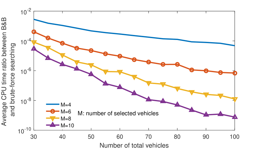
As the B&B method is guaranteed to find the optimal solution. The performance of this method is evaluated by the computational complexity compared with that of the brute-force searching. Fig. 3 shows the ratio between the average CPU time of the B&B method over 100 simulations and that of the brute-force searching. Instead of actually running the simulation for the brute-force searching, which can be computationally prohibitive, the computation time is estimated by the product of the average computation time for each objective function evaluation and the required number of evaluation.
As the number of feasible solutions increases dramatically with the increase of $N$ and $M$, the B&B method saves more computation time. For $N=100$ and $M=10$, the number of feasible solutions is $C^{10}_{100}=1.73\times 10^{13}$, while the average computation time using the B&B method is only 0.5 s on MATLAB 2016a with an Intel i-7 6500U processor. Instead of evaluating the objective function for every possible combination, the B&B method only did $O(10^{4})$ evaluations on average, owing to the use of the bound function.

III-B Optimality of the uniform distribution

In this section, a related problem will be considered, which serves as the foundation of a CE algorithm that solves the vehicle selection problem when the non-common error variances are different. Consider the road angles as random variables drawn from some distribution, the square error (17) becomes a random variable as a function of the road angles as well as the non-common error variances. It will be proved that in the limit that the number of vehicles goes to infinity, the expectation of the geometric error $e^{2}_{0}$ is minimized if the angles of the roads on which the vehicles travel obey a uniform distribution.
Considering an arbitrary continuous distribution of the road angle $p(\theta),\theta\in[0,2\pi)$, the periodic condition should be satisfied,

$$p(0)=p(2\pi^{-}),$$ (20)

as $\theta=0$ and $\theta=2\pi$ represent the same angle.
This periodicity motivates the following Fourier series expansion,

$$p(\theta)=\frac{1}{2\pi}+\sum_{m\in Z^{*}}C_{m}exp(im\theta),$$ (21)

with

$$C_{m}=C^{*}_{-m},$$ (22)

where the integer $m$ is the summation index, the asterisk denotes the complex conjugate and $i=\sqrt{-1}$ is the imaginary unit. The constant $\frac{1}{2\pi}$ ensures that the normalization condition is satisfied.
In the limit that $N\xrightarrow{}\infty$, the leading order term of the localization error $e^{2}_{0}$ due to deviation of the geometric center can be approximated as

$$e^{2}_{0}=\frac{4w^{2}}{9}\frac{\sum_{i=1}^{N}\tan^{2}(\frac{\tilde{\theta_{i}}}{2})}{\pi^{2}}\approx\frac{w^{2}}{9}\frac{\sum_{i=1}^{N}\tilde{\theta_{i}}^{2}}{\pi^{2}},$$ (23)

where $\tilde{\theta_{i}}$ is the difference between two adjacent angles $\theta_{i+1}$ and $\theta_{i}$

$$\tilde{\theta_{i}}=\begin{cases}\theta_{i+1}-\theta_{i}&\text{for }i=1,2,...,N-1\\ \theta_{1}-\theta_{N}+2\pi&\text{for }i=N\\ \end{cases}$$ (24)

In order to derive the expectation of $e^{2}_{0}$, the distribution of $\tilde{\theta_{i}}$ denoted as $f(\tilde{\theta_{i}};N,p(\theta_{i}))$ will be considered first. $f(\tilde{\theta_{i}};N,p(\theta_{i}))$ is a nearest neighbor distribution, which satisfies the integral equation,

$$f(\tilde{\theta_{i}})=2Np(\theta_{i})(1-\int^{\tilde{\theta_{i}}}_{0}f(\tau)d\tau),$$ (25)

where the dependence on the parameters $N$ and $p(\theta_{i})$ will be omitted hereafter.
Together with the normalization condition, the solution to (25) is

$$f(\tilde{\theta_{i}})=2Np(\theta_{i})exp(-2Np(\theta_{i})\tilde{\theta_{i}}).$$ (26)

The number of vehicles $N$ and the local density of the road angles $p(\theta_{i})$ appear as parameters in the distribution. As the product $Np(\theta_{i})$ increases, the angles distributed around $\theta_{i}$ become dense, thus increasing the probability of small differential angle $\tilde{\theta_{i}}$. The expectation of $\tilde{\theta_{i}}^{2}$ is

$$E[\tilde{\theta_{i}}^{2}]=\int^{\infty}_{0}\tilde{\theta_{i}}^{2}f(\tilde{\theta_{i}})d\tilde{\theta_{i}}=\frac{1}{2N^{2}p^{2}(\theta_{i})}.$$ (27)

Combining (23) and (27), the expectation of $e^{2}_{0}$ can be derived as follows,

$$E_{\theta}[e^{2}_{0}]=\frac{w^{2}}{9\pi^{2}}\sum^{N}_{i=1}E[\tilde{\theta_{i}}^{2}]=\frac{w^{2}}{36N\pi^{2}}\sum^{N}_{i=1}\frac{1}{p^{2}(\theta_{i})}\frac{2\pi}{N}.$$ (28)

The summation in (28) can be interpreted as an integration as the number of the vehicles $N$ goes to infinity,

$$\lim\limits_{N\to\infty}{\sum^{N}_{i=1}\frac{1}{p^{2}(\theta_{i})}\frac{2\pi}{N}} =\lim\limits_{N\to\infty}{\sum^{N}_{i=1}\frac{1}{p^{2}(\theta_{i})}\Delta\theta}$$ (29)

$$=\int^{2\pi}_{0}\frac{1}{p^{2}(\theta)}d\theta.$$

The Fourier expansion of $\frac{1}{p^{2}(\theta)}$ can be obtained and expressed in terms of the Fourier coefficients of $p(\theta)$, assuming the deviation from the uniform distribution is infinitesimal,

$$\frac{1}{p^{2}(\theta)} =4\pi^{2}-8\pi^{3}\sum_{m\in Z^{*}}C_{m}exp(im\theta)$$ (30)

$$+16\pi^{4}(\sum_{m\in Z^{*}}C_{m}exp(im\theta))^{2}+O(C^{3}_{m}).$$

Substituting (30) into (29),

$$\lim\limits_{N\to\infty}{\sum^{N}_{i=1}\frac{1}{p^{2}(\theta_{i})}\frac{2\pi}{N}}=8\pi^{3}+32\pi^{5}\sum^{\infty}_{m=1}|C_{m}|^{2}.$$ (31)

Substituting (31) into (28),

$$E_{\theta}[e^{2}_{0}]\sim\frac{w^{2}}{36N\pi^{2}}(8\pi^{3}+32\pi^{5}\sum^{\infty}_{m=1}|C_{m}|^{2}).$$ (32)

By taking $C_{m}=0,m\in Z^{+}$, which corresponds to the uniform distribution, the expectation of the square error $E_{\theta}[e^{2}_{0}]$ is minimized.

III-C The CE method based two-step algorithm

The two-step algorithm is comprised of a heuristic pre-selection step to downsize the eligible vehicle population and a sampling-based searching step that applies the CE method for the optimization inspired by the existence of the optimal distribution, described as follows:

III-C1 Step one: pre-selection

An important observation that motivates this pre-selection is that the objective function (17) is monotonically increasing with respect to the non-common error variances $\sigma^{2}_{i},i=1,2,...,M$. If two vehicles have close road angles, i.e., $\theta_{i}\approx\theta_{j}$ and large difference of the non-common error variance, e.g., $\sigma^{2}_{i}\ll\sigma^{2}_{j}$, then it is very unlikely that selecting the $j$-th vehicle will lead to the optimal solution as substituting the $j$-th vehicle with the $i$-th vehicle would probably make the objective function smaller. The following procedure is used to eliminate those unpromising vehicles:

• For all pairs that satisfy $\sigma^{2}_{i}<\sigma^{2}_{j}$:
  Sample randomly $K$ pairs of groups of vehicles with indices: $[n_{l,1},n_{l,2}...,n_{l,M-1},i],[n_{l,1},n_{l,2}...,n_{l,M-1},j]$, where $l=1,2,...,K$, and evaluate the corresponding pairs of the objective function values $J_{l,i},J_{l,j}$.

• If $J_{l,i}<J_{l,j}$ for all $l=1,2,...,K$:
  Then eliminate the j-th vehicle from the selection candidates.

III-C2 Step two: CE method

After the pre-selection step, a CE method is applied, motivated by the existence of the optimal distribution (the uniform distribution) proved in the previous section. The CE method searches for the minimizer of the objective function by iteratively sampling from a parameterized distribution and updating the parameter according to the samples with good performance. In this particular optimization problem, a $M$-dimensional Gaussian distribution of the road angle is used, which is described by the following pseudo-code:

• Iterate until the convergence criterion (for the distribution parameters) is satisfied:

• Generate $k$ samples from the Gaussian distribution denoted as $[s_{1},s_{2},...,s_{k}]$, where each $s_{i}=[\theta_{i,1},\theta_{i,2},...,\theta_{i,M}],i=1,2,...,k$ is an $M$ dimension vector of angles that are not necessarily equal to any of the actual road angles.

• Round the angles to the nearest road angles, which leads to the rounded samples $\tilde{s}_{1},\tilde{s}_{2},...,\tilde{s}_{k}$, and evaluate the values of the objective function denoted as $J_{1},J_{2},...,J_{k}$.

• Update the mean and covariance parameter as $\mu=\frac{\sum^{k}_{i=1}I[J_{i}\geq\hat{\gamma}]\tilde{s}_{i}}{k_{\rho}}$ and $cov=\frac{\sum^{k}_{i=1}I[J_{i}\geq\hat{\gamma}](\tilde{s}_{i}-\mu)(\tilde{s}_{i}-\mu)^{T}}{k_{\rho}-1}$ [11], where $\hat{\gamma}$ is the sample $(1-\rho)$- quantile of performance, $k_{\rho}$ is the corresponding number of samples and $I$ is the indicator function.

The performance of this two-step algorithm is demonstrated on synthetic data with $N=50$ and $M=5$. In addition, the road angles are drawn from a uniform distribution and the non-common error variances are generated by $\sigma^{2}_{i}=(0.5+|v_{i}|)\mbox{ }m^{2}$, where $v_{i}\sim\mathcal{N}(0,1)$. The other parameters are: $K=10$, $k=1000$, $\rho=0.05$. The initial parameters of the Gaussian distribution are $\mu_{0}=[0,\frac{2\pi}{M},\frac{4\pi}{M},...,\frac{2(M-1)\pi}{M}]$ and $cov_{0}=diag([100(\frac{\pi}{M})^{2},100(\frac{\pi}{M})^{2}...,100(\frac{\pi}{M})^{2}]^{T}_{M\times 1})$.

Figure 4: Performance of the optimization algorithm; the total number of feasible solution is $C^{5}_{50}=2,118,760$.

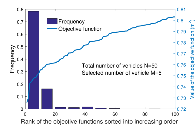
Fig. 4 shows the distribution of the optimization results sorted into increasing order of the objective function values based on 1000 simulations and the sorted values of the objective function corresponding to the best 100 combinations of $M$ vehicles (blue line). The total number of feasible solution is $C^{5}_{50}=2,118,760$, while the solutions found by the algorithm are among the best 20 ones in 95% of the cases and all the results are within the best 100 ones. The average computation time is 1.6 s for each simulation.
The pre-selection step plays an important role in achieving this performance. Without the pre-selection, the CE algorithm would waste a lot of searching on the samples that are unpromising to be optimal. As a result, the performance would degrade.

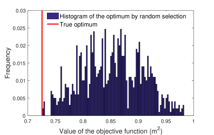
The performance of random searching based on 1000 simulations is shown in Fig. 5 for a comparison with the CE method. In each simulation, the objective function is evaluated on $N_{r}$ randomly selected combinations of $M$ vehicles, and the optimal value is the minimum among these $N_{r}$ values. The computation time and performance of this random searching depends on the fixed parameter $N_{r}$. A large $N_{r}$ would take long computation time but good performance. For a fair comparison with the CE method, this parameter is determined such that the computation time is approximately equal to that required by the CE method, which is about 5000. Fig. 5 shows that only a very small percent of the optimal values obtained through the random searching are close to the true optimal value, which reflects the good performance of the CE method.

Figure 5: Performance of random searching using equivalent computation time

III-D Comparison between the two optimization algorithms

In the previous sections, two optimization algorithms have been presented. Their scopes of application and performances are summarized here.
The B&B method is applied to the case where all the vehicles have the same non-common error variance. Although it is rare, in practice, to have exactly same non-common error variance for all the connected vehicles, the B&B method is expected to find a near optimal solution as long as the variances are approximately the same. The B&B method is a deterministic searching algorithm, which is guaranteed to find the optimal solution as long as the assumptions are satisfied. In the worst case, it would be necessary to search the solution space exhaustively, which would result in exponential computational complexity. In practice, however, the B&B method takes much less time than the brute-force searching does.
In contrast, the CE method with the pre-selection can also be applied when the vehicles have different non-common error variances. It is a stochastic algorithm, which does not guarantee an optimal solution. In practice, however, it finds solutions of high quality. The computational complexity is fixed once the parameters of the problem are given.
For vehicle selection problems of practical scales, the average computational time of both these two algorithms is of $O(1)$ s. Thus they are promising for real-time application.

IV CONCLUSIONS

In this paper, a theoretical framework for evaluating and optimizing the effect of road constraints on the CMM localization accuracy is established. The major contributions and findings of this work are summarized:

1. A closed-form expression that expresses the mean square localization error in terms of the road angles and non-common error is derived based on a simple CMM rule, which serves as the foundation of the vehicle optimal selection problem. Based on this expression, it is proved that the optimal distribution of road angles that minimizes the localization error is the uniform distribution.

2. A B&B algorithm and a CE algorithm are developed to select the optimal group of vehicles that minimizes the localization error. The B&B algorithm can efficiently find the optimal group when all the vehicles have the same non-common error variance, while the CE algorithm can efficiently find a near optimal group when the vehicles have different non-common error variances.

References

- [1] V. L. Knoop, P. F. de Bakker, C. C. J. M. Tiberius, and B. van Arem, “Lane determination with gps precise point positioning,” IEEE Transactions on Intelligent Transportation Systems, vol. PP, no. 99, pp. 1–11, 2017.
- [2] T. Speth, A. Kamann, T. Brandmeier, and U. Jumar, “Precise relative ego-positioning by stand-alone rtk-gps,” in 2016 13th Workshop on Positioning, Navigation and Communications (WPNC), Oct 2016, pp. 1–6.
- [3] I. M. Zendjebil, F. Ababsa, J. Y. Didier, and M. Mallem, “A gps-imu-camera modelization and calibration for 3d localization dedicated to outdoor mobile applications,” in ICCAS 2010, Oct 2010, pp. 1580–1585.
- [4] K. Lassoued, P. Bonnifait, and I. Fantoni, “Cooperative localization of vehicles sharing gnss pseudoranges corrections with no base station using set inversion,” in 2016 IEEE Intelligent Vehicles Symposium (IV), June 2016, pp. 496–501.
- [5] M. Rohani, D. Gingras, and D. Gruyer, “A novel approach for improved vehicular positioning using cooperative map matching and dynamic base station dgps concept,” IEEE Transactions on Intelligent Transportation Systems, vol. 17, no. 1, pp. 230–239, 2016.
- [6] M. Shen, D. Zhao, J. Sun, and H. Peng, “Improving localization accuracy in connected vehicle networks using rao-blackwellized particle filters: Theory, simulations, and experiments,” arXiv preprint arXiv:1702.05792, 2017.
- [7] M. Shen, D. Zhao, and J. Sun, “Enhancement of low-cost gnss localization in connected vehicle networks using rao-blackwellized particle filters,” in Intelligent Transportation Systems (ITSC), 2016 IEEE 19th International Conference on. IEEE, 2016, pp. 834–840.
- [8] K. Ramachandran, M. Gruteser, R. Onishi, and T. Hikita, “Experimental analysis of broadcast reliability in dense vehicular networks,” IEEE Vehicular Technology Magazine, vol. 2, no. 4, pp. 26–32, 2007.
- [9] M. Shen, D. Zhao, and J. Sun, “The impact of road configuration on v2v-based cooperative localization,” in IEEE 85th Vehicular Technology Conference (VTC). IEEE, 2017.
- [10] J. Clausen, “Branch and bound algorithms-principles and examples,” Department of Computer Science, University of Copenhagen, pp. 1–30, 1999.
- [11] Z. I. Botev, D. P. Kroese, R. Y. Rubinstein, P. L Ecuyer et al., “The cross-entropy method for optimization,” Machine Learning: Theory and Applications, V. Govindaraju and CR Rao, Eds, Chennai: Elsevier BV, vol. 31, pp. 35–59, 2013.