Microstructure under the Microscope: Tools to Survive and Thrive in The Age of (Too Much) Information

IHS Markit / City University of Hong Kong

March 18, 2024

Microstructure, Marketstructure, Microscope, Dimension Reduction, Distance Measure, Covariance, Distribution, Uncertainty

JEL Codes: D53 Financial Markets; G17 Financial Forecasting and Simulation; C43 Index Numbers and Aggregation

1 Abstract

Market Microstructure is the investigation of the process and protocols that govern the exchange of assets with the objective of reducing frictions that can impede the transfer. In financial markets, where there is an abundance of recorded information, this translates to the study of the dynamic relationships between observed variables, such as price, volume and spread, and hidden constituents, such as transaction costs and volatility, that hold sway over the efficient functioning of the system.

“My dear, here we must process as much data as we can, just to stay in business. And if you wish to make a profit you must process atleast twice as much data.” - Red Queen to Alice in Hedge-Fund-Land.

Necessity is the mother of all invention / creation / innovation, but the often forgotten father is frustration. In this age of (Too Much) Information, it is imperative to uncover nuggets of knowledge (signal) from buckets of nonsense (noise).

To aid in this effort to extract meaning from chaos and to gain a better understanding of the relationships between financial variables, we summarize the application of the theoretical results from (Kashyap 2016b) to microstructure studies. The central concept rests on a novel methodology based on the marriage between the Bhattacharyya distance, a measure of similarity across distributions, and the Johnson Lindenstrauss Lemma, a technique for dimension reduction, providing us with a simple yet powerful tool that allows comparisons between data-sets representing any two distributions.

We provide an empirical illustration using prices, volumes and volatilities across seven countries and three different continents. The degree to which different markets or sub groups of securities have different measures of their corresponding distributions tells us the extent to which they are different. This can aid investors looking for diversification or looking for more of the same thing.

In Indian mythology, it is believed that in each era, God takes on an avatar or reincarnation to fight the main source of evil in that epoch and to restore the balance between good and bad. In this age of too much information and complexity, perhaps the supreme being needs to be born as a data scientist, conceivably with an apt nickname, the Infoman. Until higher powers intervene and provide the ultimate solution to completely eliminate information overload, we have to make do with marginal methods, such as this composition, to reduce information.

As we wait for the perfect solution, it is worth meditating upon what superior beings would do when faced with a complex situation, such as the one we are in. It is said that the Universe is but the Brahma’s (Creator’s) dream. Research (Effort / Struggle) can help us understand this world; Sleep (Ease / Peace of Mind) can help us create our own world. A lesson from close by and down under: We need to “Do Some Yoga and Sleep Like A Koala”.

2 Objectively Subjective

A hall mark of the social sciences is the lack of objectivity. Here we assert that objectivity is with respect to comparisons done by different participants and that a comparison is a precursor to a decision.

Conjecture 1.

Despite the several advances in the social sciences, we have yet to discover an objective measuring stick for comparison, a so called, True Comparison Theory, which can be an aid for arriving at objective decisions.

The search for such a theory could again be compared, to the medieval alchemists’ obsession with turning everything into gold (Kashyap 2014a). For our present purposes, the lack of such an objective measure means that the difference in comparisons, as assessed by different participants, can effect different decisions under the same set of circumstances. Hence, despite all the uncertainty in the social sciences, the one thing we can be almost certain about is the subjectivity in all decision making.

2.1 Merry-Go-Round of Comparisons, Decisions and Actions

This lack of an objective measure for comparisons, makes people react at varying degrees and at varying speeds, as they make their subjective decisions. A decision gives rise to an action and subjectivity in the comparison means differing decisions and hence unpredictable actions. This inability to make consistent predictions in the social sciences explains the growing trend towards comprehending better and deciphering the decision process and the subsequent actions, by collecting more information across the entire cycle of comparisons, decisions and actions. Another feature of the social sciences is that the actions of participants affects the state of the system, effecting a state transfer which perpetuates another merry-go-round of comparisons, decisions and actions from the participants involved. This means, more the participants, more the changes to the system, more the actions and more the information that is generated to be gathered.

Restricted to the particular sub-universe of economic and financial theory, this translates to the lack of an objective measuring stick of value, a so called, True Value Theory. This lack of an objective measure of value, (hereafter, value will be synonymously referred to as the price of a financial instrument), makes prices react at differing degrees and at varying velocities to the pull of different macro and micro factors.

(Lawson 1985) argues that the Keynesian view on uncertainty (that it is generally impossible, even in probabilistic terms, to evaluate the future outcomes of all possible current actions; Keynes 1937; 1971; 1973), far from being innocuous or destructive of economic analysis in general, can give rise to research programs incorporating, amongst other things, a view of rational behavior under uncertainty, which could be potentially fruitful. (McManus and Hastings 2005) clarify the wide range of uncertainties that affect complex engineering systems and present a framework to understand the risks (and opportunities) they create and the strategies system designers can use to mitigate or take advantage of them. These viewpoints hold many lessons for policy designers in the social sciences and could be instructive for researchers looking to create methods to compare complex systems, keeping in mind the caveats of dynamic social systems.

2.2 Interplay of Information and Intelligence

On the surface, it would seem that there is a repetitive nature to portfolio management, which we can term "The Circle of Investment" (Kashyap 2014b), making it highly amenable to automation. But we need to remind ourselves that the reiterations happen under the purview of a special kind of uncertainty that applies to the social sciences. (Kashyap 2014a) goes into greater depth on how the accuracy of predictions and the popularity of generalizations might be inversely related in the social sciences. In the practice of investment management and also to aid other business decisions, more data sources are being created, collected and used along with increasing automation and artificial intelligence.

If Alice and Red Queen of the Wonderland fame (Carroll 1865; 1871; End-note 2) were to visit Hedge-Fund-Land (or even Business-Land), the following modification of their popular conversation would aptly describe the situation today, “My dear, here we must process as much data as we can, just to stay in business. And if you wish to make a profit you must process atleast twice as much data.”

We could also apply this to HFT-Land and say: “My dear, here we must trade as fast as we can, just to stay in business. And if you wish to make a profit, you must trade atleast twice as fast as that.”, while reminiscing that the jury is still out on whether HFT is Good, Bad or Just Ugly and Unimportant.

In Academic-Land, this would become: “My dear, here we must process as much data (and include as many strange symbols or obfuscating terms) as we can, just to create a working paper. And if you wish to make a publication you must process atleast twice as much data (and include atleast twice as many strange characters or obfuscating expressions).”

We currently lack a proper understanding of how, in some instances, our brains (or minds; and right now it seems we don’t know the difference!) make the leap of learning from information to knowledge to wisdom (See Mill 1829; Mazur 2015 for more about learning and behavior). The problem of creating artificial intelligence can be a child’s play, depending on which adult’s brainpower acts as our gold standard. Perhaps, the real challenge is to replicate the curiosity and learning an infant displays. Intellect might be a byproduct of Inquisitiveness, demonstrating another instance of an unintended yet welcome consequence (Kashyap 2016e). This brings up the question of Art and Science in the practice of asset management (and everything else in life?); which are more related than we probably realize, “Art is Science that we don’t know about; Science is Art restricted to a set of symbols governed by a growing number of rules” (Kashyap 2014a).

While the similarities between art and science, should give us hope; we need to face the realities of the situation. Right now, arguably, in most cases, we (including computers and intelligent machines?) can barely make the jump from the information to the knowledge stage; even with the use of cutting / (bleeding?) edge technology and tools. This exemplifies three things:

1. We are still in the information age. As another route to establishing this, consider this: Information is Hidden; Knowledge is Exchanged or Bartered; Wisdom is Dispersed. Surely we are still in the Information Age since a disproportionate amount of our actions are geared towards accumulating unique data-sets for the sole benefits of the accumulators.

2. Automating the movement to a higher level of learning, which is necessary for dealing with certain doses of uncertainty, is still far away.

3. Some of us missed the memo that the best of humanity are actually robots in disguise, living amongst us.

Hence, it is not Manager versus Machine (Portfolio Manager vs Computing Machine or MAN vs MAC, in short; End-notes 3, 4, 5). Not even MAN and MAC against the MPC (Microsoft Personal Computer; End-notes 6, 7, 8)? It is MAN, MAC and the MPC against increasing complexity! (Also in scope are other computing platforms from the past, present and the future: Williams 1997; Ifrah, Harding, Bellos and Wood 2000; Ceruzzi 2003; End-notes 9, 10, 11, 12). This increasing complexity and information explosion is perhaps due to the increasing number of complex actions perpetrated by the actors that comprise the financial system. The human mind will be obsolete if machines can fully manage assets and we would have bigger problems on our hands than who is managing our money. We need, and will continue to need, massive computing power to mostly separate the signal from the noise.

2.3 Simply Too Complex

(Simon 1962) points out that any attempt to seek properties common to many sorts of complex systems (physical, biological or social), would lead to a theory of hierarchy since a large proportion of complex systems observed in nature exhibit hierarchic structure; that a complex system is composed of subsystems that, in turn, have their own subsystems, and so on. This might hold a clue to the miracle that our minds perform; abstracting away from the dots that make up a picture, to fully visualizing the image, that seems far removed from the pieces that give form and meaning to it. To helps us gain a better understanding of the relationships between financial variables, we construct a metric built from smaller parts, but gives optimal benefits when seen from a higher level. Contrary to what conventional big picture conversations suggest, as the spectator steps back and the distance from the picture increases, the image becomes smaller yet clearer.

As a first step, we recognize that one possible categorization (Kashyap 2016c) of different fields can be done by the set of questions a particular field attempts to answer. The answers to the questions posed by any domain can come from anywhere or from phenomenon studied under a combination of many other disciplines. Hence, the answers to the questions posed under the realm of economics and finance can come from seemingly diverse subjects, such as, physics, biology, mathematics, chemistry, and so on. As we embark on the journey to apply the knowledge from other fields to finance, we need to be aware that finance is Simply Too Complex, since all of finance, through time, has involved three simple outcomes - “Buy, Sell or Hold”. The complications are mainly to get to these results.

Definition 1.

Market Microstructure is the investigation of the process and protocols that govern the exchange of assets with the objective of reducing frictions that can impede the transfer.

In financial markets, where there is an abundance of recorded information, this translates to the study of the dynamic relationships between observed variables, such as price, volume and spread, and hidden constituents, such as transaction costs and volatility, that hold sway over the efficient functioning of the system (Kashyap 2015b).

While it might be possible to observe historical trends (or other attributes) and make comparisons across fewer number of entities, in large systems where there are numerous components or contributing elements, this can be a daunting task. If time travel were to become possible, time series would no longer be relevant. We are accustomed to using time and money as our units of measurement. Time and money are but means to an end. If we start viewing efforts and the world in terms of what we hope to accomplish ultimately, it might lead to better results.

In this present paper, we put aside the fundamental question of whether we need complicated models or merely better morals and present quantitative measures across aggregations of smaller elements that can aid decision makers by providing simple yet powerful metrics to compare groups of entities. The results draw upon sources from statistics, probability, economics / finance, communication systems, pattern recognition and information theory; becoming one example of how elements of different fields can be combined to provide answers to the questions raised by a particular field. The degree to which different markets or sub groups of securities have different measures of their corresponding distributions tells us the extent to which they are different. This can aid investors looking for diversification or looking for more of the same thing.

2.4 Nuggets of Knowledge from Buckets of Nonsense

Necessity is the mother of all invention / creation / innovation, but the often forgotten father is frustration. In this age of (Too Much) Information, it is imperative to uncover nuggets of knowledge from buckets of nonsense.

To aid in this effort to extract meaning from chaos, we summarize the application of the theoretical results from (Kashyap 2016b) to microstructure studies. The central concept rests on a novel methodology based on the marriage between the Bhattacharyya distance, a measure of similarity across distributions, and the Johnson Lindenstrauss Lemma, a technique for dimension reduction, providing us with a simple yet powerful tool that allows comparisons between data-sets representing any two distributions, perhaps also becoming, to our limited knowledge, an example of perfect matrimony.

We return to Sergei Bubka, our Icon of Uncertainty (Kashyap 2016a). As a refresher for the younger generation, he broke the pole vault world record 35 times. We can think of regulatory change or the utilization of newer methods and techniques as raising the bar. Each time the bar is raised, the spirit of Sergei Bubka, in all of us, will find a way over it. The varying behavior of participants in a social system will give rise to unintended consequences (Kashyap 2016e) and as long as participants are free to observe the results and modify their actions, this effect will persist. (Kashyap 2015a) consider ways to reduce the complexity of social systems, which could be one way to mitigate the effect of unintended outcomes. While attempts at designing less complex systems are worthy endeavors, reduced complexity might be hard to accomplish in certain instances and despite successfully reducing complexity, alternate techniques at dealing with uncertainty are commendable complementary pursuits (Kashyap 2016d).

Asset price bubbles are seductive but scary when they burst. What we learn from the story of Beauty and the Beast is that they must coexist; we need to learn to love the beast before we can uncover the beauty. Similarly bubbles and busts must be close to one another. If we find that microstructure variables, especially implicit trading costs, are showing steady movement, the change in transaction costs could be a signal of a potential building up of a bubble and a later bust. Our study will allow the comparison of trading costs across aggregations of individual securities, allowing inferences to be drawn across sectors or markets, enabling us to find early indications of bubbles building up in corners of the economy.

2.5 The Miracle of Mathematics

Lastly on a cautionary note, since the concepts mentioned below involve non-trivial mathematical principles, we point out that the source of most (all) human conflict (and misunderstanding) is not because of what is said (written) and heard (read), but is partly due to how something is said and mostly because of the difference between what is said and heard and what is meant and understood. We list a few different ways of describing what mathematics is and perhaps why it is miraculously magical most of the time but minutiae some times, that could be relegated to an appendix to be safely ignored.

1. Mathematics is built on one simple operation, addition, making it a fractal with addition as its starting point.

2. Mathematics has become complex because of the confusion that different notations, assumptions not made explicit and missed steps can create.

3. Mathematics without the steps is like a treasure hunt without the clues.

4. Mathematics is like a swimsuit model wearing a Burkha; we need to see beyond the symbols and the surface to appreciate the beauty.

In a complex system, deriving equations can be a daunting exercise, and not to mention, of limited practical validity. Hence, to supplements equations, we need to envision the numerous unknowns that can cause equations to go awry; while remembering that a candle in the dark is better than nothing at all. Pondering on the sources of uncertainty and the tools we have to capture it, might lead us to believe that, either, the level of our mathematical knowledge is not advanced enough, or, we are using the wrong methods. The dichotomy between logic and randomness is a topic for another time.

3 Methodological Fundamentals

3.1 Notation and Terminology for Key Results

• $D_{BC}\left(p_{i},p_{i}^{\prime}\right)$, the Bhattacharyya Distance between two multinomial populations each consisting of $k$ categories classes with associated probabilities $p_{1},p_{2},...,p_{k}$ and $p_{1}^{\prime},p_{2}^{\prime},...,p_{k}^{\prime}$ respectively.

• $\rho\left(p_{i},p_{i}^{\prime}\right)$, the Bhattacharyya Coefficient.

• $D_{BC-N}(p,q)$ is the Bhattacharyya distance between $p$ and $q$ normal distributions or classes.

• $D_{BC-MN}\left(p_{1},p_{2}\right)$ is the Bhattacharyya distance between two multivariate normal distributions, $\boldsymbol{p_{1}},\boldsymbol{p_{2}}$ where $\boldsymbol{p_{i}}\sim\mathcal{N}(\boldsymbol{\mu}_{i},\,\boldsymbol{\Sigma}_{i})$.

• $D_{BC-TN}(p,q)$ is the Bhattacharyya distance between $p$ and $q$ truncated normal distributions or classes.

• $D_{BC-TMN}\left(p_{1},p_{2}\right)$ is the Bhattacharyya distance between two truncated multivariate normal distributions, $\boldsymbol{p_{1}},\boldsymbol{p_{2}}$ where $\boldsymbol{p_{i}}\sim\mathcal{N}(\boldsymbol{\mu}_{i},\,\boldsymbol{\Sigma}_{i},\,\boldsymbol{a}_{i},\,\boldsymbol{b}_{i})$.

3.2 Bhattacharyya Distance

We use the Bhattacharyya distance (Bhattacharyya 1943, 1946) as a measure of similarity or dissimilarity between the probability distributions of the two entities we are looking to compare. These entities could be two securities, groups of securities, markets or any statistical populations that we are interested in studying. The Bhattacharyya distance is defined as the negative logarithm of the Bhattacharyya coefficient.

$$D_{BC}\left(p_{i},p_{i}^{\prime}\right)=-\ln\left[\rho\left(p_{i},p_{i}^{\prime}\right)\right]$$

The Bhattacharyya coefficient is calculated as shown below for discrete and continuous probability distributions.

$$\rho\left(p_{i},p_{i}^{\prime}\right)=\sum_{i}^{k}\sqrt{p_{i}p_{i}^{\prime}}$$

$$\rho\left(p_{i},p_{i}^{\prime}\right)=\int\sqrt{p_{i}\left(x\right)p_{i}^{\prime}\left(x\right)}dx$$

Bhattacharyya’s original interpretation of the measure was geometric (Derpanis 2008). He considered two multinomial populations each consisting of $k$ categories classes with associated probabilities $p_{1},p_{2},...,p_{k}$ and $p_{1}^{\prime},p_{2}^{\prime},...,p_{k}^{\prime}$ respectively. Then, as $\sum_{i}^{k}p_{i}=1$ and $\sum_{i}^{k}p_{i}^{\prime}=1$, he noted that $(\sqrt{p_{1}},...,\sqrt{p_{k}})$ and $(\sqrt{p_{1}^{\prime}},...,\sqrt{p_{k}^{\prime}})$ could be considered as the direction cosines of two vectors in $k-$dimensional space referred to a system of orthogonal co-ordinate axes. As a measure of divergence between the two populations Bhattacharyya used the square of the angle between the two position vectors. If $\theta$ is the angle between the vectors then:

$$\rho\left(p_{i},p_{i}^{\prime}\right)=cos\theta=\sum_{i}^{k}\sqrt{p_{i}p_{i}^{\prime}}$$

Thus if the two populations are identical: $cos\theta=1$ corresponding to $\theta=0$, hence we see the intuitive motivation behind the definition as the vectors are co-linear. Bhattacharyya further showed that by passing to the limiting case a measure of divergence could be obtained between two populations defined in any way given that the two populations have the same number of variates. The value of coefficient then lies between $0$ and $1$.

$$0\leq\rho\left(p_{i},p_{i}^{\prime}\right)\leq=1$$

$$0\leq D_{BC}\left(p_{i},p_{i}^{\prime}\right)\leq\infty$$

We get the following formulae (Lee and Bretschneider 2012) for the Bhattacharyya distance when applied to the case of two uni-variate normal distributions.

$$D_{BC-N}(p,q)=\frac{1}{4}\ln\left(\frac{1}{4}\left(\frac{\sigma_{p}^{2}}{\sigma_{q}^{2}}+\frac{\sigma_{q}^{2}}{\sigma_{p}^{2}}+2\right)\right)+\frac{1}{4}\left(\frac{(\mu_{p}-\mu_{q})^{2}}{\sigma_{p}^{2}+\sigma_{q}^{2}}\right)$$

$\sigma_{p}$ is the variance of the $p-$th distribution,

$\mu_{p}$ is the mean of the $p-$th distribution, and

$p,q$ are two different distributions.

The original paper on the Bhattacharyya distance (Bhattacharyya 1943) mentions a natural extension to the case of more than two populations. For an $M$ population system, each with $k$ random variates, the definition of the coefficient becomes,

$$\rho\left(p_{1},p_{2},...,p_{M}\right)=\int\cdots\int\left[p_{1}\left(x\right)p_{2}\left(x\right)...p_{M}\left(x\right)\right]^{\frac{1}{M}}dx_{1}\cdots dx_{k}$$

For two multivariate normal distributions, $\boldsymbol{p_{1}},\boldsymbol{p_{2}}$ where $\boldsymbol{p_{i}}\sim\mathcal{N}(\boldsymbol{\mu}_{i},\,\boldsymbol{\Sigma}_{i}),$

$$D_{BC-MN}\left(p_{1},p_{2}\right)=\frac{1}{8}(\boldsymbol{\mu}_{1}-\boldsymbol{\mu}_{2})^{T}\boldsymbol{\Sigma}^{-1}(\boldsymbol{\mu}_{1}-\boldsymbol{\mu}_{2})+\frac{1}{2}\ln\,\left(\frac{\det\boldsymbol{\Sigma}}{\sqrt{\det\boldsymbol{\Sigma}_{1}\,\det\boldsymbol{\Sigma}_{2}}}\right),$$

$\boldsymbol{\mu}_{i}$ and $\boldsymbol{\Sigma}_{i}$ are the means and covariances of the distributions, and $\boldsymbol{\Sigma}=\frac{\boldsymbol{\Sigma}_{1}+\boldsymbol{\Sigma}_{2}}{2}$. We need to keep in mind that a discrete sample could be stored in matrices of the form $A$ and $B$, where, $n$ is the number of observations and $m$ denotes the number of variables captured by the two matrices.

$$\boldsymbol{A_{m\times n}}\sim\mathcal{N}\left(\boldsymbol{\mu_{1}},\boldsymbol{\varSigma_{1}}\right)$$

$$\boldsymbol{B_{m\times n}}\sim\mathcal{N}\left(\boldsymbol{\mu_{2}},\boldsymbol{\varSigma_{2}}\right)$$

3.3 Dimension Reduction

A key requirement to apply the Bhattacharyya distance in practice is to have data-sets with the same number of dimensions. (Fodor 2002; Burges 2009; Sorzano, Vargas and Montano 2014) are comprehensive collections of methodologies aimed at reducing the dimensions of a data-set using Principal Component Analysis or Singular Value Decomposition and related techniques. (Johnson and Lindenstrauss 1984) proved a fundamental result (JL Lemma) that says that any $n$ point subset of Euclidean space can be embedded in $k=O(log\frac{n}{\epsilon^{2}})$ dimensions without distorting the distances between any pair of points by more than a factor of $\left(1\pm\epsilon\right)$, for any $0<\epsilon<1$. Whereas principal component analysis is only useful when the original data points are inherently low dimensional, the JL Lemma requires absolutely no assumption on the original data. Also, note that the final data points have no dependence on $d$, the dimensions of the original data which could live in an arbitrarily high dimension. We use the version of the bounds for the dimensions of the transformed subspace given in (Frankl and Maehara 1988; 1990; Dasgupta and Gupta 1999).

Lemma 1.

For any $0<\epsilon<1$ and any integer $n$, let $k$ be a positive integer such that

$$k\geq 4\left(\frac{\epsilon^{2}}{2}-\frac{\epsilon^{3}}{3}\right)^{-1}\ln n$$

Then for any set $V$ of $n$ points in $\boldsymbol{R}^{d}$, there is a map $f:\boldsymbol{R}^{d}\rightarrow\boldsymbol{R}^{k}$ such that for all $u,v\in V$,

$$\left(1-\epsilon\right)\|u-v\|^{2}\leq\|f\left(u\right)-f\left(v\right)\|^{2}\leq\left(1+\epsilon\right)\|u-v\|^{2}$$

Furthermore, this map can be found in randomized polynomial time and one such map is $f=\frac{1}{\sqrt{k}}Ax$ where, $x\in\boldsymbol{R}^{d}$ and $A$ is a $k\times d$ matrix in which each entry is sampled i.i.d from a Gaussian $N\left(0,1\right)$ distribution.

(Kashyap 2016b) provides expressions for the density functions after dimension transformation when considering log normal distributions, truncated normal and truncated multivariate normal distributions (Appendix A: 8). These results are applicable in the context of many variables observed in real life such as stock prices, heart rates and volatilities, which do not take on negative values. For completeness, we also include the expression for the dimension transformed normal distribution. A relationship between covariance and distance measures is also derived. An asset pricing and one biological application show the limitless possibilities such a comparison affords. Some pointers for implementation and R code snippets for the Johnson Lindenstrauss matrix transformation and a modification to the routine currently available to calculate the Bhattacharyya distance are also listed. This modification allows much larger numbers and dimensions to be handled, by utilizing the properties of logarithms and the eigen values of a matrix.

4 From Symbols to Numbers, Empirical Illustrations across Markets

We illustrate several examples of how this measure could be used to compare different countries based on the time series variables across all equity securities traded in that market. Our data sample contains prices (open, close, high and low) and trading volumes for most of the securities from six different markets from Jan 01, 2014 to May 28, 2014 (Figure 1a). Singapore with 566 securities is the market with the least number of traded securities. Even if we reduce the dimension of all the other markets with more number of securities, for a proper comparison of these markets, we would need more than two years worth of data. Hence as a simplification, we first reduce the dimension of the matrix holding the prices or volumes for each market using principal component analysis (PCA; see Shlens 2014) reduction, so that the number of tickers retained would be comparable to the number of days for which we have data. We report the results of using distance measures over the full sample after PCA reduction.

We report the full matrix and not just the upper or lower matrix since the PCA reduction we do takes the first country, reduces the dimensions upto a certain number of significant digits and then reduces the dimension of the second country to match the number of dimensions of the first country. For example, this would mean that comparing AUS and SGP is not exactly the same as comparing SGP and AUS. As a safety step before calculating the distance, which requires the same dimensions for the structures holding data for the two entities being compared, we could perform dimension reduction using JL Lemma if the dimensions of the two countries differs after the PCA reduction. We repeat the calculations for different number of significant digits of the PCA reduction. This shows the fine granularity of the results that our distance comparison produces and highlights the issue that with PCA reduction there is loss of information, since with different number of significant digits employed in the PCA reduction, we get the result that different markets are similar.

We illustrate another example, where we compare a randomly selected sub universe of securities in each market, so that the number of tickers retained would be comparable to the number of days for which we have data. This approach could also be used when groups of securities are being compared within the same market, a very common scenario when deciding on the group of securities to invest in a market as opposed to deciding which markets to invest in. Such an approach would be highly useful for index construction or comparison across sectors within a market.

We report the full matrix for the same reason as explained earlier and perform multiple iterations when reducing the dimension using the JL Lemma. A key observation is that the magnitude of the distances are very different when using PCA reduction and when using dimension reduction, due to the loss of information that comes with the PCA technique. It is apparent that using dimension reduction via the JL Lemma produces consistent results, since the same pairs of markets are seen to be similar in different iterations. It is worth remembering that in each iteration of the JL Lemma dimension transformation we multiply by a different random matrix and hence the distance is slightly different in each iteration but within the bound established by JL Lemma. When the distance is somewhat close between two pairs of entities, we could observe an inconsistency due to the JL Lemma transformation in successive iterations.

Lastly, we calculate sixty day moving volatilities on the close price and trading volume and calculate the distance measure over the full sample and also across each of the randomly selected sub-samples.

4.1 Speaking Volumes Of: Comparison of Trading Volumes

The results of the volume comparison over the full sample are shown in Figure 1b. For example, in Figure 1b, AUS - GBR are the most similar markets when two significant digits are used and AUS - GBR are the most similar with six significant digits. In this case the PCA and JL Lemma dimension reduction give similar results.

The random sample results are shown in Figure 2. The left table (Figure 2a) is for PCA reduction on a randomly chosen sub universe and the right table (Figure 2b) is for dimension reduction using JL Lemma for the same sub universe.

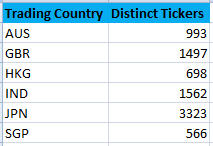
(a) Markets and Tickers Count

(b) Volume PCA Dimension Reduction

Figure 1: Security Count by Market / Volume Distance Measures over Full Sample

(a) Volume PCA Dimension Reduction

(b) Volume JL Lemma Dimension Reduction

Figure 2: Volume Distance Measures over Randomly Chosen Sub Universe

4.2 A Pricey Prescription: Comparison of Prices (Open, Close, High and Low)

4.2.1 Open Close

The results of a comparison between open and close prices over the full sample are shown in Figures 3, 3a, 3b. For example, in Figure 3b, AUS - SGP are the most similar markets when two significant digits are used and AUS - HKG are the most similar with six significant digits. The similarities between open and close prices, in terms of the distance measure, are also easily observed.

The random sample results are shown in Figures 4, 5. The left table (Figures 4a, 5a) is for PCA reduction on a randomly chosen sub universe and the right table (Figures 4b, 5b) is for dimension reduction using JL Lemma for the same sub universe. In Figure 5b, AUS - IND are the most similar in iteration one and also in iteration five.

(a) Open PCA Dimension Reduction

(b) Close PCA Dimension Reduction

Figure 3: Open / Close Distance Measures over Full Sample

(a) Open PCA Dimension Reduction

(b) Open JL Lemma Dimension Reduction

Figure 4: Open Distance Measures over Randomly Chosen Sub Universe

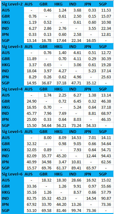
(a) Close PCA Dimension Reduction

(b) Close JL Lemma Dimension Reduction

Figure 5: Close Distance Measures over Randomly Chosen Sub Universe

4.2.2 High Low

The results of a comparison between high and low prices over the full sample are shown in Figures 6, 6a, 6b. For example, in Figure 6a, AUS - SGP are the most similar markets when two significant digits are used and AUS - HKG are the most similar with six significant digits. The similarities between high and low prices are also easily observed.

The random sample results are shown in Figures 7, 8. The left table (Figures 7a, 8a) is for PCA reduction on a randomly chosen sub universe and the right table (Figures 7b, 8b) is for dimension reduction using JL Lemma for the same sub universe. In Figures 7b and 8b, AUS - IND are the most similar in iteration one and also in iteration five.

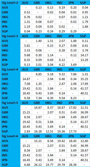
(a) High PCA Dimension Reduction

(b) Low PCA Dimension Reduction

Figure 6: High / Low Distance Measures over Full Sample

(a) High PCA Dimension Reduction

(b) High JL Lemma Dimension Reduction

Figure 7: High Distance Measures over Randomly Chosen Sub Universe

(a) Low PCA Dimension Reduction

(b) Low JL Lemma Dimension Reduction

Figure 8: Low Distance Measures over Randomly Chosen Sub Universe

4.3 Taming the (Volatility) Skew: Comparison of Close Price / Volume Volatilities

The results of a comparison between close price volatilities and volume volatilities over the full sample are shown in Figures 9, 9a, 9b. For example, in Figure 9a, AUS - GBR are the most similar markets when two significant digits are used and AUS - HKG are the most similar with six significant digits. In Figure 9b, AUS - GBR - IND are equally similar markets when two significant digits are used and AUS - GBR are the most similar with six significant digits. The difference in magnitudes of the distance measures for prices, volumes and volatilities is also easily observed. What this indicates is that, prices are from the most dissimilar or distant distributions, volatilities are less similar and volumes are from the most similar or overlapping distributions. As also observed in the volume comparisons, volume volatility comparisons give seemingly similar results when PCA or JL Lemma dimension reductions are used. By considering the price volatilities, and creating portfolios of instruments that have dissimilar volatility distributions, we could reduce the overall risk or variance of the portfolio returns, becoming one potential way of mitigating the effects of wild volatility swings.

The random sample results are shown in Figures 10, 11. The left table (Figures 10a, 11a) is for PCA reduction on a randomly chosen sub universe and the right table (Figures 10b, 11b) is for dimension reduction using JL Lemma for the same sub universe. In Figure 10b AUS - SGP are the most similar in iteration one and also in iteration five. In Figure 11b, AUS - SGP are the most similar in iteration one and AUS- GBR in iteration five.

(a) Close Volatility PCA Dimension Reduction

(b) Volume Volatility PCA Dimension Reduction

Figure 9: Close / Volume Volatility Distance Measures over Full Sample

(a) Close Volatility PCA Dimension Reduction

(b) Close Volatility JL Lemma Dimension Reduction

Figure 10: Close Volatility Distance Measures over Randomly Chosen Sub Universe

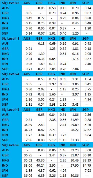
(a) Volume Volatility PCA Dimension Reduction

(b) Volume Volatility JL Lemma Dimension Reduction

Figure 11: Volume Volatility Distance Measures over Randomly Chosen Sub Universe

5 Possibilities for Future Research

1. A key limitation of this study is that we have reduced dimensions using PCA or randomly sampled a sub matrix from the overall data-set so that the length of time series available is in the range of the number of securities that could be compared. Using a longer time series for the variables would be a useful extension and a real application would benefit immensely from more history.

2. We have used the simple formula for the Bhattacharyya distance applicable to multivariate normal distributions. The formulae we have developed over a truncated multivariate normal distribution or using a Normal Log-Normal Mixture could give more accurate results. Again, later works should look into tests that can establish which of the distributions would apply depending on the data-set under consideration.

3. For each market we have looked at seven variables, open, close, low, high, volume, close volatility and volume volatility. These variables can be combined using the expression for the multinomial distance to get a complete representation of which markets are more similar than others. We aim to develop this methodology and illustrate these techniques further in later works.

4. Once we have the similarity measures across groups of securities, portfolios could be constructed to see how sensitive they are to different explanatory factors and then performance benchmarks could be used to guage the risk return relationship.

6 Conclusions

We have discussed how the combination of the Bhattacharyya distance and the Johnson Lindenstrauss Lemma provides us with a practical and novel methodology that allows comparisons between any two probability distributions. This approach can help in the comparison of systems that generate prices, quantities and aid in the analysis of shopping patterns and understanding consumer behavior. The systems could be goods transacted at different shopping malls or trade flows across entire countries. Study of traffic congestion, road accidents and other fatalities across two regions could be performed to get an idea of similarities and seek common answers where such simplifications might be applicable. Clearly, this methodology lends itself to numerous applications outside the realm of finance and economics.

We have illustrated the comparison of prices, volumes and volatilities across six different markets from three continents demonstrating the power this methodology holds for big (small?) picture decision making.

In Indian mythology (End-note 13; Zimmer 1972; Doniger 1976; Rao 1993; Flood 1996; Parrinder 1997; Swami 2011), it is believed that in each era, God takes on an avatar or reincarnation to fight the main source of evil in that epoch and to restore the balance between good and bad. In this age of too much information and complexity, perhaps the supreme being needs to be born as a data scientist, conceivably with an apt superhero nickname, the Infoman (For society’s fascination with superheroes or superhumans see: Eco and Chilton 1972; Reynolds 1992; Fingeroth 2004; Haslem, Ndalianis and Mackie 2007; Coogan 2009). Until higher powers intervene and provide the ultimate solution to completely eliminate information overload, we have to make do with marginal methods to reduce information, such as this composition.

As we wait for the perfect solution, it is worth meditating upon what superior beings would do when faced with a complex situation, such as the one we are in. It is said that the Universe is but the Brahma’s (Creator’s) dream (Barnett 1907; Ramamurthi 1995; Ghatage 2010). Research (Effort / Struggle) can help us understand this world; Sleep (Ease / Peace of Mind) can help us create our own world. We just need to be mindful that the most rosy and well intentioned dreams can have unintended consequences (Kashyap 2016e) and turn to nightmares (Nolan 2010; Lehrer 2010; Kashyap 2016f).

Native to Australia (End-note 15), “Koalas spend about 4.7 hours eating, 4 minutes traveling, 4.8 hours resting while awake and 14.5 hours sleeping in a 24-hour period” - (Nagy and Martin1985). See also (Smith 1979; Moyal 2008). The benefits of yoga on sleep quality are well documented (End-note 14; Cohen, Warneke, Fouladi, Rodriguez and Chaoul-Reich 2004; Khalsa 2004; Manjunath and Telles 2005; Chen, Chen, Chao, Hung, Lin and Li 2009; Vera, Manzaneque, Maldonado, Carranque, Rodriguez, Blanca and Morell 2009).

A lesson from close by and down under: We need to “Do Some Yoga and Sleep Like A Koala” (Figure 12). With that, we present a list of sleeping aids in section 7.

Figure 12: Sleeping Like A Koala

7 Sleeping Aids (Notes and References)

1. Dr. Yong Wang, Dr. Isabel Yan, Dr. Vikas Kakkar, Dr. Fred Kwan, Dr. William Case, Dr. Srikant Marakani, Dr. Qiang Zhang, Dr. Costel Andonie, Dr. Jeff Hong, Dr. Guangwu Liu, Dr. Humphrey Tung and Dr. Xu Han at the City University of Hong Kong provided advice and more importantly encouragement to explore and where possible apply cross disciplinary techniques. The views and opinions expressed in this article, along with any mistakes, are mine alone and do not necessarily reflect the official policy or position of either of my affiliations or any other agency.

2. The Red Queen’s race is an incident that appears in Lewis Carroll’s Through the Looking-Glass and involves the Red Queen, a representation of a Queen in chess, and Alice constantly running but remaining in the same spot.

   "Well, in our country," said Alice, still panting a little, "you’d generally get to somewhere else, if you run very fast for a long time, as we’ve been doing."

   "A slow sort of country!" said the Queen. "Now, here, you see, it takes all the running you can do, to keep in the same place. If you want to get somewhere else, you must run at least twice as fast as that!"

   The Red Queen’s Race, Wikipedia Link

   This quote is commonly attributed as being from Alice in Wonderland as: “My dear, here we must run as fast as we can, just to stay in place. And if you wish to go anywhere you must run twice as fast as that.”

3. Portfolio Manager, Wikipedia Link

4. Universal Computing Machine, Wikipedia Link

5. Computer, Wikipedia Link

6. MAC or Macintosh, Wikipedia Link

7. Personal Computer, Wikipedia Link

8. MAC vs MPC, Wikipedia Link

9. History Computing, Wikipedia Link

10. Computing Platform, Wikipedia Link

11. Cloud Computing, Wikipedia Link

12. Quantum Computing, Wikipedia Link

13. Avatar or Reincarnation, Wikipedia Link

14. Yoga, Wikipedia Link

15. Australia or Down Under, Wikipedia Link

16. Barnett, L. D. (1907). The Brahma Knowledge. An Outline of the Philosophy of the Vedanta as Set Forth by the Upanishads and by Sankara. Wisdom of the East series. E.P. Dutton Publishing, Boston, Massachusetts.

17. Bhattacharyya, A. (1943). On a Measure of Divergence Between Two Statistical Populations Defined by their Probability Distributions, Bull. Calcutta Math. Soc., 35, pp. 99-110.

18. Bhattacharyya, A. (1946). On a measure of divergence between two multinomial populations. Sankhyā: The Indian Journal of Statistics, 401-406.

19. Burges, C. J. (2009). Dimension reduction: A guided tour. Machine Learning, 2(4), 275-365.

20. Burkardt, J. (2014). The Truncated Normal Distribution. Department of Scientific Computing Website, Florida State University.

21. Carroll, L. (1865). (2012 Reprint) Alice’s adventures in wonderland. Random House, Penguin Random House, Manhattan, New York.

22. Carroll, L. (1871). (2009 Reprint) Through the looking glass: And what Alice found there. Random House, Penguin Random House, Manhattan, New York.

23. Ceruzzi, P. E. (2003). A history of modern computing. MIT press.

24. Chen, K. M., Chen, M. H., Chao, H. C., Hung, H. M., Lin, H. S., & Li, C. H. (2009). Sleep quality, depression state, and health status of older adults after silver yoga exercises: cluster randomized trial. International journal of nursing studies, 46(2), 154-163.

25. Chiani, M., Dardari, D., & Simon, M. K. (2003). New exponential bounds and approximations for the computation of error probability in fading channels. Wireless Communications, IEEE Transactions on, 2(4), 840-845.

26. Clark, P. K. (1973). A subordinated stochastic process model with finite variance for speculative prices. Econometrica: journal of the Econometric Society, 135-155.

27. Cody, W. J. (1969). Rational Chebyshev approximations for the error function. Mathematics of Computation, 23(107), 631-637.

28. Cohen, L., Warneke, C., Fouladi, R. T., Rodriguez, M., & Chaoul-Reich, A. (2004). Psychological adjustment and sleep quality in a randomized trial of the effects of a Tibetan yoga intervention in patients with lymphoma. Cancer, 100(10), 2253-2260.

29. Coogan, P. (2009). The Definition of the Superhero. A comics studies reader, 77.

30. Dasgupta, S., & Gupta, A. (1999). An elementary proof of the Johnson-Lindenstrauss lemma. International Computer Science Institute, Technical Report, 99-006.

31. Derpanis, K. G. (2008). The Bhattacharyya Measure. Mendeley Computer, 1(4), 1990-1992.

32. Doniger, W. (1976). The origins of evil in Hindu mythology (No. 6). Univ of California Press.

33. Eco, U., & Chilton, N. (1972). The myth of Superman.

34. Fingeroth, D. (2004). Superman on the Couch: What Superheroes Really Tell Us about Ourselves and Our Society. A&C Black.

35. Frankl, P., & Maehara, H. (1988). The Johnson-Lindenstrauss lemma and the sphericity of some graphs. Journal of Combinatorial Theory, Series B, 44(3), 355-362.

36. Frankl, P., & Maehara, H. (1990). Some geometric applications of the beta distribution. Annals of the Institute of Statistical Mathematics, 42(3), 463-474.

37. Flood, G. D. (1996). An introduction to Hinduism. Cambridge University Press.

38. Fodor, I. K. (2002). A survey of dimension reduction techniques. Technical Report UCRL-ID-148494, Lawrence Livermore National Laboratory.

39. Ghatage, S. (2010). Brahma’s Dream. Anchor Canada, Penguin Random House, Manhattan, New York.

40. Haslem, W., Ndalianis, A., & Mackie, C. J. (Eds.). (2007). Super/Heroes: From Hercules to Superman. New Academia Publishing, LLC.

41. Horrace, W. C. (2005). Some results on the multivariate truncated normal distribution. Journal of Multivariate Analysis, 94(1), 209-221.

42. Ifrah, G., Harding, E. F., Bellos, D., & Wood, S. (2000). The universal history of computing: From the abacus to quantum computing. John Wiley & Sons, Inc.

43. Johnson, W. B., & Lindenstrauss, J. (1984). Extensions of Lipschitz mappings into a Hilbert space. Contemporary mathematics, 26(189-206), 1.

44. Kashyap, R. (2014a). Dynamic Multi-Factor Bid–Offer Adjustment Model. The Journal of Trading, 9(3), 42-55.

45. Kashyap, R. (2014b). The Circle of Investment. International Journal of Economics and Finance, 6(5), 244-263.

46. Kashyap, R. (2015a). Financial Services, Economic Growth and Well-Being: A Four Pronged Study. Indian Journal of Finance, 9(1), 9-22.

47. Kashyap, R. (2015b). A Tale of Two Consequences. The Journal of Trading, 10(4), 51-95.

48. Kashyap, R. (2016a). Hong Kong - Shanghai Connect / Hong Kong - Beijing Disconnect (?), Scaling the Great Wall of Chinese Securities Trading Costs. The Journal of Trading, 11(3), 81-134.

49. Kashyap, R. (2016b). Combining Dimension Reduction, Distance Measures and Covariance. Working Paper.

50. Kashyap, R. (2016c). Solving the Equity Risk Premium Puzzle and Inching Towards a Theory of Everything. Working Paper.

51. Kashyap, R. (2016d). Fighting Uncertainty with Uncertainty. Working Paper.

52. Kashyap, R. (2016e). Notes on Uncertainty, Unintended Consequences and Everything Else. Working Paper.

53. Kashyap, R. (2016f). The American Dream, An Unsustainable Nightmare. Working Paper.

54. Kattumannil, S. K. (2009). On Stein’s identity and its applications. Statistics & Probability Letters, 79(12), 1444-1449.

55. Keynes, J. M. (1937). The General Theory of Employment. The Quarterly Journal of Economics, 51(2), 209-223.

56. Keynes, J. M. (1971). The Collected Writings of John Maynard Keynes: In 2 Volumes. A Treatise on Money. The Applied Theory of Money. Macmillan for the Royal Economic Society.

57. Keynes, J. M. (1973). A treatise on probability, the collected writings of John Maynard Keynes, vol. VIII.

58. Khalsa, S. B. S. (2004). Treatment of chronic insomnia with yoga: A preliminary study with sleep–wake diaries. Applied psychophysiology and biofeedback, 29(4), 269-278.

59. Kiani, M., Panaretos, J., Psarakis, S., & Saleem, M. (2008). Approximations to the normal distribution function and an extended table for the mean range of the normal variables.

60. Kimeldorf, G., & Sampson, A. (1973). A class of covariance inequalities. Journal of the American Statistical Association, 68(341), 228-230.

61. Lawson, T. (1985). Uncertainty and economic analysis. The Economic Journal, 95(380), 909-927.

62. Lee, K. Y., & Bretschneider, T. R. (2012). Separability Measures of Target Classes for Polarimetric Synthetic Aperture Radar Imagery. Asian Journal of Geoinformatics, 12(2).

63. Lehrer, J. (2010). The Neuroscience of Inception. Wired 26 Jul. 2010. Web. 13 Aug. 2013.

64. Manjunath, N. K., & Telles, S. (2005). Influence of Yoga & Ayurveda on self-rated sleep in a geriatric population. Indian Journal of Medical Research, 121(5), 683.

65. Mazur, J. E. (2015). Learning and behavior. Psychology Press.

66. McManus, H., & Hastings, D. (2005, July). 3.4. 1 A Framework for Understanding Uncertainty and its Mitigation and Exploitation in Complex Systems. In INCOSE International Symposium (Vol. 15, No. 1, pp. 484-503).

67. Mill, J. (1829). Analysis of the Phenomena of the Human Mind (Vol. 1, 2). Longmans, Green, Reader, and Dyer.

68. Miranda, M. J., & Fackler, P. L. (2002). Applied Computational Economics and Finance.

69. Moyal, A. (Ed.). (2008). Koala: a historical biography. CSIRO PUBLISHING.

70. Nagy, K. A., & Martin, R. W. (1985). Field Metabolic Rate, Water Flux, Food Consumption and Time Budget of Koalas, Phascolarctos Cinereus (Marsupialia: Phascolarctidae) in Victoria. Australian Journal of Zoology, 33(5), 655-665.

71. Nolan, C. (2010). Inception [film]. Warner Bros.: Los Angeles, CA, USA.

72. Parrinder, E. G. (1997). Avatar and incarnation: the divine in human form in the world’s religions. Oneworld Publications Limited.

73. Ramamurthi, B. (1995). The fourth state of consciousness: The Thuriya Avastha. Psychiatry and clinical neurosciences, 49(2), 107-110.

74. Rao, T. G. (1993). Elements of Hindu iconography. Motilal Banarsidass Publisher.

75. Reynolds, R. (1992). Super heroes: A modern mythology. Univ. Press of Mississippi.

76. Rubinstein, M. E. (1973). A comparative statics analysis of risk premiums. The Journal of Business, 46(4), 605-615.

77. Rubinstein, M. (1976). The valuation of uncertain income streams and the pricing of options. The Bell Journal of Economics, 407-425.

78. Shlens, J. (2014). A tutorial on principal component analysis. arXiv preprint arXiv:1404.1100.

79. Simon, H. A. (1962). The Architecture of Complexity. Proceedings of the American Philosophical Society, 106(6), 467-482.

80. Smith, M. (1979). Behaviour of the Koala, Phascolarctos Cinereus Goldfuss, in Captivity. 1. Non-Social Behaviour. Wildlife Research, 6(2), 117-129.

81. Soranzo, A., & Epure, E. (2014). Very simply explicitly invertible approximations of normal cumulative and normal quantile function. Applied Mathematical Sciences, 8(87), 4323-4341.

82. Sorzano, C. O. S., Vargas, J., & Montano, A. P. (2014). A survey of dimensionality reduction techniques. arXiv preprint arXiv:1403.2877.

83. Stein, C. M. (1973). Estimation of the mean of a multivariate normal distribution. Proceedings of the Prague Symposium of Asymptotic Statistics.

84. Stein, C. M. (1981). Estimation of the mean of a multivariate normal distribution. The annals of Statistics, 1135-1151.

85. Swami, B. (2011). Bhagavad Gita as it is. The Bhaktivedanta book trust, Mumbai, India.

86. Tauchen, G. E., & Pitts, M. (1983). The Price Variability-Volume Relationship on Speculative Markets. Econometrica, 51(2), 485-505.

87. Teerapabolarn, K. (2013). Stein’s identity for discrete distributions. International Journal of Pure and Applied Mathematics, 83(4), 565.

88. Vera, F. M., Manzaneque, J. M., Maldonado, E. F., Carranque, G. A., Rodriguez, F. M., Blanca, M. J., & Morell, M. (2009). Subjective sleep quality and hormonal modulation in long-term yoga practitioners. Biological psychology, 81(3), 164-168.

89. Williams, M. R. (1997). A history of computing technology. IEEE Computer Society Press.

90. Yang, M. (2008). Normal log-normal mixture, leptokurtosis and skewness. Applied Economics Letters, 15(9), 737-742.

91. Zimmer, H. R. (1972). Myths and symbols in Indian art and civilization (Vol. 6). Princeton University Press.

92. Zogheib, B., & Hlynka, M. (2009). Approximations of the Standard Normal Distribution. University of Windsor, Department of Mathematics and Statistics.

8 Appendix A: Dimension Reduction, Distance Measures and Covariance

All the results below are from (Kashyap 2016b). Other useful references are pointed in the relevant sections below.

8.1 Normal Log-Normal Mixture

Transforming log-normal multi-variate variables into a lower dimension by multiplication with an independent normal distribution (See Lemma 1) results in the sum of variables with a normal log-normal mixture, (Clark 1973; Tauchen and Pitts 1983; Yang 2008), evaluation of which requires numerical techniques (Miranda and Fackler 2002).

A random variable, $U$, would be termed a normal log-normal mixture if it is of the form,

$$U=Xe^{Y}$$

where, $X$ and $Y$ are random variables with correlation coefficient, $\rho$ satisfying the below,

$$\left[\begin{array}[]{c}X\\ Y\end{array}\right]\sim N\left(\left[\begin{array}[]{c}\mu_{X}\\ \mu_{Y}\end{array}\right],\left[\begin{array}[]{cc}\sigma_{X}^{2}&\rho\sigma_{X}\sigma_{Y}\\ \rho\sigma_{X}\sigma_{Y}&\sigma_{Y}^{2}\end{array}\right]\right)$$

We note that for $\sigma_{Y}=0$ when $Y$ degenerates to a constant, this is just the distribution of $X$ and $\rho$ is unidentified.

To transform a column vector with $d$ observations of a random variable into a lower dimension of order, $k<d$, we can multiply the column vector with a matrix, $A\sim N(0;\frac{1}{k})$ of dimension $k\times d$.

Lemma 2.

A dimension transformation of $d$ observations of a log-normal variable into a lower dimension, $k$, using Lemma 1, yields a probability density function which is the sum of random variables with a normal log-normal mixture, given by the convolution,

$$f_{S}\left(s\right)=f_{U_{1}}\left(u_{1}\right)*f_{U_{2}}\left(u_{2}\right)*...*f_{U_{k}}\left(u_{k}\right)$$

$$\text{Here, }f_{U_{i}}\left(u_{i}\right)=\frac{\sqrt{k}}{2\pi\sigma_{Y_{i}}}\int_{-\infty}^{\infty}\;e^{-y-\frac{ku_{i}^{2}}{2e^{2y}}-\frac{\left[y-\mu_{Y_{i}}\right]^{2}}{2\sigma_{Y_{i}}^{2}}}dy$$

$$U_{i}=X_{i}e^{Y_{i}}$$

$$\left[\begin{array}[]{c}X_{i}\\ Y_{i}\end{array}\right]\sim N\left(\left[\begin{array}[]{c}0\\ \mu_{Y_{i}}\end{array}\right],\left[\begin{array}[]{cc}\frac{1}{k}&0\\ 0&\sigma_{Y_{i}}^{2}\end{array}\right]\right)$$

The convolution of two probability densities arises when we have the sum of two independent random variables, $Z=X+Y$. The density of $Z,\;h_{Z}\left(z\right)$ is given by,

$${\displaystyle h_{Z}\left(z\right)=\left(f_{X}\text{\textasteriskcentered}f_{Y}\right)\left(z\right)=f_{X}\left(x\right)*f_{Y}\left(y\right)=\int_{-\infty}^{\infty}f_{X}\left(z-y\right)*f_{Y}\left(y\right)dy=\int_{-\infty}^{\infty}f_{X}\left(x\right)*f_{Y}\left(z-x\right)dx}$$

When the number of independent random variables being added is more than two, or the reduced dimension after the Lemma 1 transformation is more than two, $k>2$, then we can take the convolution of the density resulting after the convolution of the first two random variables, with the density of the third variable and so on in a pair wise manner, till we have the final density.

8.2 Normal Normal Product

For completeness, we illustrate how dimension reduction would work on a data-set containing random variables that have normal distributions. This can serve as a useful benchmark given the wide usage of the normal distribution and can be an independently useful result, though most variables observed in real life are normally not so normal.

Lemma 3.

A dimension transformation of $d$ observations of a normal variable into a lower dimension, $k$, using Lemma 1, yields a probability density function which is the sum of random variables with a normal normal product distribution, given by the convolution,

$$f_{S}\left(s\right)=f_{U_{1}}\left(u_{1}\right)*f_{U_{2}}\left(u_{2}\right)*...*f_{U_{k}}\left(u_{k}\right)$$

$$\text{Here, }f_{U_{i}}\left(u_{i}\right)=\int_{-\infty}^{\infty}\left(\frac{1}{\left|x\right|}\right)\frac{1}{\sigma_{Y_{i}}\sqrt{2\pi}}\;e^{-\frac{\left(x-\mu_{Y_{i}}\right)^{2}}{2\sigma_{Y_{i}}^{2}}}\sqrt{\frac{k}{2\pi}}\;e^{-\frac{k\left(\frac{u_{i}}{x}\right)^{2}}{2}}dx$$

$$U_{i}=X_{i}Y_{i}$$

$$\left[\begin{array}[]{c}X_{i}\\ Y_{i}\end{array}\right]\sim N\left(\left[\begin{array}[]{c}0\\ \mu_{Y_{i}}\end{array}\right],\left[\begin{array}[]{cc}\frac{1}{k}&0\\ 0&\sigma_{Y_{i}}^{2}\end{array}\right]\right)$$

8.3 Truncated Normal Distribution

A truncated normal distribution is the probability distribution of a normally distributed random variable whose value is either bounded below, above or both (Horrace 2005; Burkardt 2014). (Kiani, Panaretos, Psarakis and Saleem 2008; Zogheib and Hlynka 2009; Soranzo and Epure 2014) list some of the numerous techniques to calculate the normal cumulative distribution. Approximations to the error function are also feasible options (Cody 1969; Chiani, Dardari and Simon 2003). Despite the truncation, this could be a potent extension when it is known a-priori that the values a variable can take are almost surely bounded.

Suppose $X\sim N(\mu,\sigma^{2})$ has a normal distribution and lies within the interval $X\in(a,b),\;-\infty\leq a<b\leq\infty$. Then $X$ conditional on $a<X<b$ has a truncated normal distribution. Its probability density function, $f_{X}$, for $a\leq x\leq b$ , is given by

$$f_{X}\left(x\mid\mu,\sigma^{2},a,b\right)=\begin{cases}\frac{\frac{1}{\sigma}\phi\left(\frac{x-\mu}{\sigma}\right)}{\Phi\left(\frac{b-\mu}{\sigma}\right)-\Phi\left(\frac{a-\mu}{\sigma}\right)}&\quad;a\leq x\leq b\\ 0&;\text{otherwise}\end{cases}$$

Here, ${\scriptstyle{\phi(\xi)=\frac{1}{\sqrt{2\pi}}\exp{(-\frac{1}{2}\xi^{2}})}}$ is the probability density function of the standard normal distribution and ${\scriptstyle{\Phi(\cdot)}}$ is its cumulative distribution function. There is an understanding that if ${\scriptstyle{b=\infty}\ }$, then ${\scriptstyle{\Phi(\frac{b-\mu}{\sigma})=1}}$, and similarly, if ${\scriptstyle{a=-\infty}}$ , then ${\scriptstyle{\Phi(\frac{a-\mu}{\sigma})=0}}$.

Lemma 4.

The Bhattacharyya distance, when we have truncated normal distributions $p,q$ that do not overlap, is zero and when they overlap, it is given by

$$D_{BC-TN}(p,q) = \frac{1}{4}\left(\frac{(\mu_{p}-\mu_{q})^{2}}{\sigma_{p}^{2}+\sigma_{q}^{2}}\right)+\frac{1}{4}\ln\left(\frac{1}{4}\left(\frac{\sigma_{p}^{2}}{\sigma_{q}^{2}}+\frac{\sigma_{q}^{2}}{\sigma_{p}^{2}}+2\right)\right)$$

$$+\frac{1}{2}\ln\left[\Phi\left(\frac{b-\mu_{p}}{\sigma_{p}}\right)-\Phi\left(\frac{a-\mu_{p}}{\sigma_{p}}\right)\right]+\frac{1}{2}\ln\left[\Phi\left(\frac{d-\mu_{q}}{\sigma_{q}}\right)-\Phi\left(\frac{c-\mu_{q}}{\sigma_{q}}\right)\right]$$

$$-\ln\left\{\Phi\left[\frac{u-\nu}{\varsigma}\right]-\Phi\left[\frac{l-\nu}{\varsigma}\right]\right\}$$

Here,

$$p\sim N\left(\mu_{p},\sigma_{p}^{2},a,b\right)\;;\;q\sim N\left(\mu_{q},\sigma_{q}^{2},c,d\right)$$

$$l=\min\left(a,c\right)\;;\;u=\min\left(b,d\right)$$

$$\nu=\frac{\left(\mu_{p}\sigma_{q}^{2}+\mu_{q}\sigma_{p}^{2}\right)}{\left(\sigma_{p}^{2}+\sigma_{q}^{2}\right)}\;;\;\varsigma=\sqrt{\frac{2\sigma_{p}^{2}\sigma_{q}^{2}}{\left(\sigma_{p}^{2}+\sigma_{q}^{2}\right)}}$$

8.4 Truncated Multivariate Normal Distribution

Similarly, a truncated multivariate normal distribution $\boldsymbol{X}$ has the density function,

$$f_{\mathbf{X}}\left(x_{1},\ldots,x_{k}\mid\boldsymbol{\mu_{p}},\,\boldsymbol{\Sigma_{p}},\,\boldsymbol{a},\,\boldsymbol{b}\right)=\frac{\exp\left(-\frac{1}{2}\left({\mathbf{x}}-{\boldsymbol{\mu_{p}}})^{\mathrm{T}}\right){\boldsymbol{\Sigma_{p}}}^{-1}\left({\mathbf{x}}-{\boldsymbol{\mu_{p}}}\right)\right)}{\int_{\boldsymbol{a}}^{\boldsymbol{b}}\exp\left(-\frac{1}{2}\left({\mathbf{x}}-{\boldsymbol{\mu_{p}}})^{\mathrm{T}}\right){\boldsymbol{\Sigma_{p}}}^{-1}\left({\mathbf{x}}-{\boldsymbol{\mu_{p}}}\right)\right)d\boldsymbol{x};\;\boldsymbol{x}\in\boldsymbol{R}_{\boldsymbol{a}\leq\boldsymbol{x}\leq\boldsymbol{b}}^{k}}$$

Here, $\boldsymbol{\mu_{p}}$ is the mean vector and $\boldsymbol{\Sigma_{p}}$ is the symmetric positive definite covariance matrix of the $\boldsymbol{p}$ distribution and the integral is a $k$ dimensional integral with lower and upper bounds given by the vectors $\left(\boldsymbol{a},\boldsymbol{b}\right)$ and $\boldsymbol{\boldsymbol{x}\in\boldsymbol{R}_{\boldsymbol{a}\leq\boldsymbol{x}\leq\boldsymbol{b}}^{k}}$ .

Lemma 5.

The Bhattacharyya coefficient when we have truncated multivariate normal distributions $\boldsymbol{p},\boldsymbol{q}$ and all the $k$ dimensions have some overlap, is given by

$$D_{BC-TMN}\left(\boldsymbol{p},\boldsymbol{q}\right) = \frac{1}{8}(\boldsymbol{\mu_{p}}-\boldsymbol{\mu_{q}})^{T}\boldsymbol{\Sigma}^{-1}(\boldsymbol{\mu_{p}}-\boldsymbol{\mu_{q}})+\frac{1}{2}\ln\,\left(\frac{\det\boldsymbol{\Sigma}}{\sqrt{\det\boldsymbol{\Sigma_{p}}\,\det\boldsymbol{\Sigma_{q}}}}\right)$$

$$+\frac{1}{2}\ln\left[\frac{1}{\sqrt{(2\pi)^{k}\left(|\boldsymbol{\Sigma_{p}}|\right)}}\int_{\boldsymbol{a}}^{\boldsymbol{b}}\exp\left(-\frac{1}{2}\left({\mathbf{x}}-{\boldsymbol{\mu_{p}}})^{\mathrm{T}}\right){\boldsymbol{\Sigma_{p}}}^{-1}\left({\mathbf{x}}-{\boldsymbol{\mu_{p}}}\right)\right)d\boldsymbol{x};\;\boldsymbol{x}\in\boldsymbol{R}_{\boldsymbol{a}\leq\boldsymbol{x}\leq\boldsymbol{b}}^{k}\right]$$

$$+\frac{1}{2}\ln\left[\frac{1}{\sqrt{(2\pi)^{k}\left(|\boldsymbol{\Sigma_{q}}|\right)}}\int_{\boldsymbol{c}}^{\boldsymbol{d}}\exp\left(-\frac{1}{2}\left({\mathbf{x}}-{\boldsymbol{\mu_{\boldsymbol{q}}}})^{\mathrm{T}}\right){\boldsymbol{\Sigma_{\boldsymbol{q}}}}^{-1}\left({\mathbf{x}}-{\boldsymbol{\mu_{\boldsymbol{q}}}}\right)\right)d\boldsymbol{x};\;\boldsymbol{x}\in\boldsymbol{R}_{\boldsymbol{\boldsymbol{c}}\leq\boldsymbol{x}\leq\boldsymbol{d}}^{k}\right]$$

$$-\ln\left[\frac{1}{\sqrt{(2\pi)^{k}\det\left({\boldsymbol{\Sigma_{p}}}{\boldsymbol{\Sigma}}^{-1}{\boldsymbol{\Sigma_{q}}}\right)}}\right.$$

$$\left.\int_{\boldsymbol{l}}^{\boldsymbol{u}}\exp\left(-\frac{1}{2}\left\{\left({\mathbf{x}-\mathbf{m}}\right)^{\mathrm{T}}\left({\boldsymbol{\Sigma_{q}}}^{-1}\left[{\boldsymbol{\Sigma}}\right]{\boldsymbol{\Sigma_{p}}}^{-1}\right)\left({\mathbf{x}-\mathbf{m}}\right)\right\}\right)d\boldsymbol{x};\;\boldsymbol{x}\in\boldsymbol{R}_{\boldsymbol{\min\left(a,\boldsymbol{c}\right)}\leq\boldsymbol{x}\leq\boldsymbol{\min\left(b,d\right)}}^{k}\vphantom{\frac{\sqrt{(2\pi)^{k}\det\left({\boldsymbol{\Sigma_{p}}}^{-1}\right)}}{\sqrt{(2\pi)^{k}\det\left({\boldsymbol{\Sigma_{p}}}^{-1}\right)}}}\right]$$

Here,

$$\boldsymbol{p}\sim N\left(\boldsymbol{\mu_{p}},\,\boldsymbol{\Sigma_{p}},\,\boldsymbol{a},\,\boldsymbol{b}\right)$$

$$\boldsymbol{q}\sim N\left(\boldsymbol{\mu_{\boldsymbol{q}}},\,\boldsymbol{\Sigma_{\boldsymbol{q}}},\,\boldsymbol{c},\,\boldsymbol{d}\right)$$

$$\boldsymbol{u=\min\left(b,d\right)}\;;\;\boldsymbol{l=\min\left(a,c\right)}$$

$${\mathbf{m}}=\left[\left({\boldsymbol{\mu_{p}}}^{\mathrm{T}}{\boldsymbol{\Sigma_{p}}}^{-1}+{\boldsymbol{\mu_{q}}}^{\mathrm{T}}{\boldsymbol{\Sigma_{q}}}^{-1}\right)\left({\boldsymbol{\Sigma_{p}}}^{-1}+{\boldsymbol{\Sigma_{q}}}^{-1}\right)^{-1}\right]^{\mathrm{T}}$$

$$\boldsymbol{\Sigma}=\frac{\boldsymbol{\Sigma_{p}}+\boldsymbol{\Sigma_{q}}}{2}$$

8.5 Covariance and Distance

The following is a general extension to Stein’s lemma (Stein 1973, 1981; Rubinstein 1973, 1976) that does not require normality, involving the covariance between a random variable and a function of another random variable. Kattumannil (2009) extends the Stein lemma by relaxing the requirement of normality. (Teerapabolarn 2013) is a further extension of this normality relaxation to discrete distributions. Another useful reference, (Kimeldorf and Sampson 1973), provides a class of inequalities between the covariance of two random variables and the variance of a function of the two random variables.

Lemma 6.

The following equations govern the relationship between the Bhattacharyya distance, $\rho\left(f_{X},f_{Y}\right)$, and the covariance between any two distributions with joint density function, $f_{XY}\left(t,u\right)$, means, $\mu_{X}\text{ and }\mu_{Y}$ and density functions $f_{X}\left(t\right)\text{ and }f_{Y}\left(t\right)$,

$$\text{Cov}\left[c\left(X\right),Y\right]=\text{Cov}\left(X,Y\right)-E\left[\sqrt{\frac{f_{Y}\left(t\right)}{f_{X}\left(t\right)}}Y\right]+\mu_{Y}\>\rho\left(f_{X},f_{Y}\right)$$

$$\text{Cov}\left(X,Y\right)+\mu_{Y}\>\rho\left(f_{X},f_{Y}\right)=E\left[c^{\prime}\left(X\right)\>g\left(X,Y\right)\right]+E\left[\sqrt{\frac{f_{Y}\left(t\right)}{f_{X}\left(t\right)}}Y\right]$$

Here,

$$c\left(t\right)=t-\sqrt{\frac{f_{Y}\left(t\right)}{f_{X}\left(t\right)}}$$

and $g\left(t,u\right)$ is a non-vanishing function such that,

$$\frac{f_{XY}^{\prime}\left(t,u\right)}{f_{XY}\left(t,u\right)}=-\frac{g^{\prime}\left(t,u\right)}{g\left(t,u\right)}+\frac{\left[\mu_{Y}-u\right]}{g\left(t,u\right)}\quad,\quad t,u\in(a,b)$$