Static Black Holes With
Back Reaction From Vacuum Energy

Pei-Ming Ho, Yoshinori Matsuo

Department of Physics and Center for Theoretical Physics,
National Taiwan University, Taipei 106, Taiwan, R.O.C.

We study spherically symmetric static solutions to the semi-classical Einstein equation sourced by the vacuum energy of quantum fields in the curved space-time of the same solution. We found solutions that are small deformations of the Schwarzschild metric for distant observers, but without horizon. Instead of being a robust feature of objects with high densities, the horizon is sensitive to the energy-momentum tensor in the near-horizon region.

1 Introduction

Since it was discovered that a black hole finally evaporates by the Hawking radiation, the information loss paradox has been a longstanding problem in black hole physics. The event horizon plays an important role in this problem, and it is assumed in many studies on the information loss paradox that the event horizon still exists even when the quantum effects are taken into account. On the other hand, there are many arguments from the viewpoint of string theory, most noticeably via the AdS/CFT duality, that the information cannot be lost by the black hole evaporation. There are also many studies that argue the absence of the horizon [1, 2, 3, 4, 5, 6, 8, 9, 10, 11, 12, 13, 14, 7, 15, 16, 17].

In this paper, we will explore the connection between the near-horizon geometry and the energy-momentum tensor. We study the back reaction from the vacuum energy-momentum tensor of quantum fields on the near-horizon geometry, and consider how the vacuum energy-momentum tensor modifies the geometry. The motivation comes from the studies with self-consistent treatment of the Hawking radiation in geometries of the black hole evaporation. Recently it was shown that no horizon forms during the gravitational collapse if the back reaction from the Hawking radiation is taken into account [8, 9, 10, 11, 12, 13, 14].

In the study of black holes, Hawking radiation is associated with a conserved energy-momentum tensor, which can be computed as the vacuum expectation value of the energy-momentum operator of quantum fields outside the horizon. Naively, this quantum correction to the energy-momentum tensor, being extremely small, should have very little effect on the black-hole horizon, which exists at a macroscopic scale. On the other hand, the formation of horizons in gravitational collapses is known to be a critical phenomenon [18]. Infinitesimal modifications to the initial condition around the critical value can make a significant difference in the final states. Indeed, we will show that in some sense the existence of horizon is very sensitive to the variation of the energy-momentum tensor.

As a first step, we will focus on static configurations with spherical symmetry in this work, and leave its generalization to dynamical processes without spherical symmetry to the future. We will demonstrate in two different models of quantum fields that the quantum correction to the energy-momentum tensor is capable of removing the horizon.

We are not claiming that an infinitesimal modification to the energy-momentum tensor leads to dramatic changes in physics. The quantum energy-momentum tensor outside a static star is extremely weak for a distant observer. Their back reaction to the geometry can indeed be neglected as a good approximation for the space-time region outside the horizon which is visible to a distant observer. On the other hand, the horizon can be deformed into a wormhole-like geometry by merely modifying the geometry within an extremely small region near the Schwarzschild radius, and the difference can be hard to distinguish for a distant observer.

The vacuum expectation value of the energy-momentum operator has been calculated in the fixed Schwarzschild background for the models that we will consider, as well as for other similar models, but its back reaction to the geometry have been ignored, or treated with insufficient rigor most of the time. The fact that the vacuum energy-momentum tensor is consistently small outside a black hole was taken by many as a confirmation that its back reaction to the background geometry through the semi-classical Einstein equation

$$G_{\mu\nu}=\kappa\langle T_{\mu\nu}\rangle$$ (1)

can be ignored. However, it is also assumed by some that the Boulware vacuum is unphysical as it has divergence at the horizon in the Schwarzschild geometry. A circular logic is sometimes used to further argue that the back reaction of the quantum effects can be ignored, since those states with large quantum effects such as the Boulware vacuum are all assumed to be unphysical. However, it is also an unnatural condition to introduce the incoming energy such that the energy-momentum tensor does not diverge at the future horizon, unless the future horizon is already proven to exist. Here, we impose the more natural initial condition that there is no incoming energy flow in the past infinity. If the Boulware vacuum is unphysical, there must be outgoing energy in future infinity and black holes cannot have static states for this initial condition. However, there is a chance to have a physical state for the Boulware vacuum if we take the back reaction from the quantum effects into account. We will show nonperturbatively that there is a solution to the semi-classical Einstein equation for the Boulware vacuum without divergence in the energy-momentum tensor, and hence, it is physically sensible to consider the Boulware vacuum.

The perturbation expansion for the semi-classical Einstein equation around the Schwarzschild background breaks down at the horizon. Due to the divergence in the Boulware vacuum, the correction term to the Schwarzschild solution also diverges at the horizon. Instead of the perturbation theory as an expansion in the Newton constant, we rely on non-perturbative analysis of the semi-classical Einstein equations. Our analysis shows that the horizon of the classical Schwarzschild solution can be deformed into a wormhole-like structure (without horizon) by an arbitrarily small correction to the energy-momentum tensor. The wormhole-like structure connects the internal region of the star to the external region well approximated by the Schwarzschild solution. We emphasize that the wormhole-like geometry is not connected to another open space (hence it is not a genuine wormhole), but to the surface of a matter sphere. We will not consider the geometry inside the matter sphere, where the energy-momentum tensor of the matter needs to be specified. Instead, we will focus on the neighborhood of the wormhole-like geometry, or other kinds of geometry that replaces the near-horizon region. In the literature, the wormhole-like geometry is also called a “bounce” or “turning point” (of the radius function $r$).

For static configurations with spherical symmetry, the event horizon is also a Killing horizon and an apparent horizon. An object falling through the horizon can never return. When the horizon is deformed into a wormhole-like structure, an object falling towards the center can always return, but only after an extremely long time. Hence, from the viewpoint of a distant observer, an “approximate horizon” still exists. In practice, an extremely long period of time beyond a certain infrared cutoff can be approximated as infinite time. The horizon can be viewed as the ideal limit in which the time for an object to come out of the approximate horizon approaches to infinity. In this sense, our conclusion that an infinitesimal modification can replace a mathematical horizon by an approximate horizon is nothing dramatic. Nevertheless, while the notion of horizon plays a crucial role in conceptual problems such as the information loss paradox, it is of crucial importance to understand how to characterize the geometry of approximate horizons and their difference from the exact horizon.

It should be noted, however, that the Killing horizon in static geometry is not directly related to the information loss paradox. This paper is aimed at exploring the local structure around the horizon and study how it is modified by quantum corrections, and the global structure is out of the scope of this paper. We will show that the Killing horizon is sometimes removed after taking into account the back reaction of the quantum effects. This does not immediately imply that the event horizon does not appear in the dynamical process of a gravitational collapse, as the notion of the event horizon for dynamical systems is quite different from that of static systems, and the horizon might be recovered due to the effect of the Hawking radiation. Therefore it is non-trivial to apply the result of this paper to the formation of black holes, which is a problem we will attack in the near future.

After setting up the basic formulation for latter discussions in Sec. 2, we revisit in Sec. 3 and Sec. 4 different models people have used to estimate the vacuum expectation value of the energy-momentum operator outside a black hole, as examples of how tiny quantum corrections can turn off the horizon. It is not of our concern whether these models are accurate. Our intention is to demonstrate the possibility for a small correction in the energy-momentum tensor to remove the horizon.

In Sec. 5, we consider generic static configurations with spherical symmetry, without assumptions on the underlying physics that determines the vacuum energy-momentum tensor. In addition to Einstein equations, we only assume that the geometry is free of singularity at macroscopic scales. (The possibility of a singularity at the origin is expected to be resolved by a UV-complete theory and is irrelevant to the low-energy physics for macroscopic phenomena.) It turns out that this regularity condition leads to clear connections between the horizon and the energy-momentum tensor at the horizon. This provides us with a context in which the results of earlier sections can be understood.

2 4D Einstein Equation in S-Wave Approximation

In this paper, we assume the validity of the 4-dimensional semi-classical Einstein equation,

$$G^{(4)}_{\mu\nu}=\kappa\langle T^{(4)}_{\mu\nu}\rangle\ ,$$ (2)

in which gravity is treated classically but the quantum effect on the energy-momentum tensor is taken into account. Assuming that the classical energy-momentum tensor vanishes outside the radius $R$ of the star, the energy-momentum tensor for $r>R$ is completely given by the expectation value $\langle T^{(4)}_{\mu\nu}\rangle$ of the quantum energy-momentum operator.

To determine the energy-momentum tensor $\langle T^{(4)}_{\mu\nu}\rangle$ outside the star, we will consider massless scalar fields as examples — except that in Sec. 5 we will consider a generic energy-momentum tensor. For simplicity, we consider only spherically symmetric configurations, and separate the angular coordinates $(\theta,\phi)$ on the 2-sphere from the temporal and radial coordinates $(x^{0},x^{1})$ as

$$ds^{2}=\sum_{\mu,\nu=0,\cdots,3}g_{\mu\nu}dx^{\mu}dx^{\nu}=\sum_{\mu,\nu=0,1}g^{(2)}_{\mu\nu}dx^{\mu}dx^{\nu}+r^{2}d\Omega^{2}\ ,$$ (3)

where $d\Omega^{2}=d\theta^{2}+\sin^{2}\theta d\phi^{2}$ is the metric on the 2-sphere. Due to spherical symmetry, we can integrate out the angular coordinates in the action for a 4-dimensional massless scalar field, and obtain its 2-dimensional effective action as

$$S_{m} =\frac{1}{2}\int d^{4}x\;\sqrt{-g}\sum_{\mu,\nu=0,\cdots,3}g^{\mu\nu}\partial_{\mu}\chi\partial_{\nu}\chi$$

$$=\frac{4\pi}{2}\int d^{2}x\;\sqrt{-g^{(2)}}\;r^{2}\sum_{\mu,\nu=0,1}g^{\mu\nu}_{(2)}\partial_{\mu}\chi\partial_{\nu}\chi\ .$$ (4)

Next, we consider the Einstein-Hilbert action. The 4-dimensional curvature can be decomposed into 2-dimensional quantities as

$$R^{(4)}=R^{(2)}-6(\partial\phi)^{2}+4\nabla^{2}\phi+2\mu^{-2}e^{2\phi}\ ,$$ (5)

where $R^{(2)}$ is the 2-dimensional scalar curvature and $\phi\equiv-\log(r/\mu)$ appears as the dilaton field in 2 dimensions. (The dilaton $\phi$ is originated from the radius $r$ of the integrated 2-sphere, and $\mu$ is an arbitrary scale parameter.) After integrating out the angular coordinates, the 4-dimensional Einstein-Hilbert action turns into the 2-dimensional effective action for the dilaton field:

$$S_{\text{EH}}=-\frac{1}{16\pi G}\int d^{2}x\;\sqrt{-g^{(2)}}\,\mu^{2}e^{-2\phi}\left[R^{(2)}+2(\partial\phi)^{2}+2\mu^{-2}e^{2\phi}\right]\ .$$ (6)

As the 2-dimensional Einstein tensor vanishes identically, the equations of motion of the dimensionally reduced action only involves the dilaton and a cosmological constant.

In Secs. 3 and 4, we will compute the vacuum energy-momentum tensor $\langle T^{(4)}_{\mu\nu}\rangle$ in different models that have been used in the literature on the study of the back reaction of Hawking radiation (e.g.[19, 20, 21, 22, 4]), and they have been assumed to capture at least the qualitative features of the problem. Those with reservations about the accuracy of these models, or any other assumption adopted in the calculation below, should also dismiss the literature based on the same assumptions, and the implication of this work would be at least this: The existence of horizon depends on the details of the energy-momentum tensor, and there is so far no rigorous proof of the presence of horizon that fully incorporates the back reaction of the vacuum energy-momentum tensor in a realistic 4-dimensional theory.

Since 4-dimensional and 2-dimensional energy-momentum tensors are defined by

$$T^{(4)}_{\mu\nu} =\frac{2}{\sqrt{-g}}\frac{\delta S_{m}}{\delta g^{\mu\nu}}\ ,$$ (7)

$$T^{(2)}_{\mu\nu} =\frac{2}{\sqrt{-g^{(2)}}}\frac{\delta S_{m}}{\delta g^{\mu\nu}_{(2)}}\ ,$$ (8)

respectively, their expectation values are related to each other (in the s-wave approximation) by

$$\langle T^{(4)}_{\mu\nu}\rangle=\frac{1}{r^{2}}\langle T^{(2)}_{\mu\nu}\rangle\qquad(\mu,\nu=0,1)$$ (9)

on the reduced 2-dimensional space-time with coordinates $(x^{0},x^{1})$. Hence the semi-classical Einstein equation (2) becomes

$$G^{(4)}_{\mu\nu}=\frac{1}{r^{2}}\langle T^{(2)}_{\mu\nu}\rangle\qquad(\mu,\nu=0,1).$$ (10)

The angular components of the 4-dimensional Einstein equation, e.g. $G^{(4)}_{\theta\theta}=\kappa\langle T_{\theta\theta}^{(4)}\rangle$, are equivalent to the equation of motion for the dilaton.

To avoid potential confusions in the discussion below, we comment that the 4-dimensional conservation law for the energy-momentum tensor

$$\nabla^{\mu}\langle T_{\mu\nu}^{(4)}\rangle=0\qquad(\mu,\nu=0,1,2,3)$$ (11)

can be expressed in terms of the 2-dimensional tensor $\langle T^{(2)}_{\mu\nu}\rangle$ as

$$\nabla^{\mu}\langle T_{\mu\nu}^{(2)}\rangle-\left(\partial_{\mu}r^{2}\right)\langle T^{(4)\theta}{}_{\theta}\rangle=0\qquad(\mu,\nu=0,1),$$ (12)

which in general violates the naive 2-dimensional conservation law

$$\nabla^{\mu}\langle T_{\mu\nu}^{(2)}\rangle=0\qquad(\mu,\nu=0,1).$$ (13)

But if we include the energy-momentum tensor of the dilaton field in $T^{(2)}_{\mu\nu}$ together with the matter field, the last term in (12) would be cancelled and the 2-dimensional conservation law (13) would hold.

3 Toy Model: 4D Energy-Momentum From 2D Scalars

In this section, we study the toy model considered by Davies, Fulling and Unruh [19] for the vacuum energy-momentum tensor outside a massive sphere. In this toy model, we replace the 4-dimensional scalar field (4) by the 2-dimensional minimally coupled massless scalar field, whose action is

$$S=\frac{1}{2}\int d^{2}x\,\sqrt{-g^{(2)}}\sum_{\mu,\nu=0,1}g^{\mu\nu}_{(2)}\partial_{\mu}\chi\partial_{\nu}\chi\ .$$ (14)

We shall compute the quantum correction $\langle T_{\mu\nu}^{(2)}\rangle$ to the energy-momentum tensor for this 2-dimensional quantum field theory and then use eq.(9) to estimate the 4-dimensional vacuum energy-momentum tensor $\langle T_{\mu\nu}^{(4)}\rangle$.

It should be noted that the 2-dimensional minimally coupled scalar (14) satisfies the 2-dimensional energy-momentum conservation law (13). Thus, according to the 4-dimensional conservation law (12), the angular components of the energy-momentum tensor for the 2-dimensional minimal scalar must vanish:

$$\langle T^{(4)}_{\theta\theta}\rangle=\langle T^{(4)}_{\phi\phi}\rangle=0\ .$$ (15)

3.1 Energy-Momentum From Weyl Anomaly

For minimally coupled scalar fields, the quantum effects for the energy-momentum tensor is essentially determined by the conformal anomaly and energy-momentum conservation. Here we review the work of Davies, Fulling and Unruh [19], where they computed the expectation value of the quantum energy-momentum tensor for the toy model described above. They did calculation in the fixed Schwarzschild background without back reaction. We will consider the back reaction of the quantum energy-momentum tensor after reviewing their work.

Consider a minimally coupled massless scalar with the action (14) for a given 2-dimensional metric. According to Davies and Fulling [31], the quantum energy-momentum operator of this 2-dimensional theory can be regularized to be consistent with energy-momentum conservation, but it breaks the conformal symmetry. The Weyl anomaly is

$$\langle T^{(2)\,\mu}{}_{\mu}\rangle=\frac{1}{24\pi}R^{(2)}\ .$$ (16)

In the conformal gauge, the metric is specified by a single function $C$ as

$$ds^{2}=-C(u,v)dudv\ ,$$ (17)

and the regularized quantum energy-momentum operator has the expectation value (for a certain quantum state to be specified below)

$$\langle T^{(2)}_{\mu\nu}\rangle=\theta_{\mu\nu}+\frac{R^{(2)}}{48\pi}g_{\mu\nu},$$ (18)

where the 2-dimensional curvature is

$$R^{(2)}=\frac{4}{C^{3}}\left(C\partial_{u}\partial_{v}C-\partial_{u}C\partial_{v}C\right),$$ (19)

and

$$\theta_{uu} =-\frac{1}{12\pi}C^{1/2}\partial_{u}^{2}C^{-1/2}\ ,$$ (20)

$$\theta_{vv} =-\frac{1}{12\pi}C^{1/2}\partial_{v}^{2}C^{-1/2}\ ,$$ (21)

$$\theta_{uv} =0\ .$$ (22)

The expressions of $\theta_{\mu\nu}$ are not given in a covariant form and do not transform covariantly under the coordinate transformation $u\rightarrow u^{\prime}(u)$, $v\rightarrow v^{\prime}(v)$ (which preserves the conformal gauge) because it is the energy-momentum tensor for a specific vacuum state. Choosing a different set of coordinates $(u,v)$ gives the energy-momentum tensor for a different state. The vacuum state with the energy-momentum tensor (18)–(22) is the one with respect to which the creation/annihilation operators in the scalar field are associated with the positive/negative frequency modes $\{e^{i\omega u},e^{i\omega v}\}$.

While the trace part of the energy-momentum tensor is fixed by the Weyl anomaly, the conservation law implies that the energy-momentum tensor for any state can always be written in the form

$$\langle T_{\mu\nu}^{(2)}\rangle=\frac{1}{48\pi}g_{\mu\nu}R^{(2)}+\theta_{\mu\nu}+\widehat{T}_{\mu\nu}\ .$$ (23)

The functions $\widehat{T}_{\mu\nu}$ are the integration constants arising from solving the equation of conservation and depend only on $u$ for outgoing modes and $v$ for incoming modes. That is,

$$\widehat{T}_{uu} =\widehat{T}_{uu}(u)\ ,$$ (24)

$$\widehat{T}_{vv} =\widehat{T}_{uu}(v)\ ,$$ (25)

$$\widehat{T}_{uv} =0\ ,$$ (26)

namely, $\widehat{T}_{uu}$ and $\widehat{T}_{vv}$ are a function of $u$ and that of $v$, respectively. The dependence of $\langle T_{\mu\nu}^{(2)}\rangle$ on the choice of states now resides in $\widehat{T}_{\mu\nu}$, which vanishes for the specific vacuum state associated with the coordinates $(u,v)$ in the way described above. They can also be fixed by the choice of boundary conditions at the spatial infinity. The conservation law and Weyl anomaly are preserved regardless of the choice of these functions.

Now we review the computation by Davies, Fulling and Unruh [19] for the quantum energy-momentum tensor outside a 4-dimensional static star without back reaction. The 4-dimensional metric for a spherically symmetric configuration can be put in the form

$$ds^{2}=-Cdu\,dv+r^{2}d\Omega^{2}\ ,$$ (27)

with two parametric functions $C(u,v)$ and $r(u,v)$. Assuming that the star is a massive thin shell of radius $r=R$, we have $C=1$ for the empty space inside the shell ($r<R$) with the light-cone coordinates denoted by $(U,V)$. When the back reaction of the vacuum energy-momentum tensor is ignored,

$$C(r)=1-\frac{2M}{r}\ ,$$ (28)

for the Schwarzschild metric outside the shell ($r>R$), where $M$ is the mass of the star. The Schwarzschild radius $a_{0}$ equals $2M$.

The continuity of the metric at $r=R$ determines the relation between the coordinate system $(U,V)$ inside the shell and the coordinate system $(u,v)$ outside the shell as

$$U=(1-2M/R)^{1/2}u\ ,\qquad V=(1-2M/R)^{1/2}v\ .$$ (29)

As they are related by a constant scaling factor for a star with constant radius $R$, the notions about positive/negative frequency modes defined by $(U,V)$ and $(u,v)$ are exactly the same.

The quantum state inside the static mass shell is expected to be the Minkowski vacuum, for which the positive/negative frequency modes are $\{e^{\pm i\omega U},e^{\pm i\omega V}\}_{\omega>0}$. For a large radius $R$, the density of the shell is small, and we expect that the quantum state to be continuous across $r=R$. In other words, the quantum state just outside the shell at $r=R$ is the vacuum state associated with the positive/negative energy modes $\{e^{\pm i\omega U},e^{\pm i\omega V}\}_{\omega>0}$, or equivalently $\{e^{\pm i\omega u},e^{\pm i\omega v}\}_{\omega>0}$.

One can use (18)–(22) to compute the energy-momentum tensor for $r>R$ directly with $C$ given by (28). The results are [19]

$$\langle T^{(2)}_{uu}\rangle =\frac{1}{24\pi}\left(\frac{3M^{2}}{2r^{4}}-\frac{M}{r^{3}}\right)\ ,$$ (30)

$$\langle T^{(2)}_{vv}\rangle =\frac{1}{24\pi}\left(\frac{3M^{2}}{2r^{4}}-\frac{M}{r^{3}}\right)\ ,$$ (31)

$$\langle T^{(2)}_{uv}\rangle =\frac{1}{24\pi}\left(\frac{2M^{2}}{r^{4}}-\frac{M}{r^{3}}\right)\ .$$ (32)

This is the energy-momentum tensor for a static star given in Ref.[19]. The associated quantum state is called the Boulware vacuum [32].

The Boulware vacuum has vanishing energy-momentum tensor at $r\rightarrow\infty$. But the energy-momentum tensor diverges at $r=2M$ in a generic local orthonormal frame due to the diverging blue-shift factor at the horizon. Hence it is conventionally assumed that the radius of the star is not allowed to be inside the Schwarzschild radius, or equivalently, that the Boulware vacuum is not physical if the star is inside the Schwarzschild radius. We will see below that, if the back reaction is taken into consideration, there is no divergence, or very large energy-momentum tensor which induces curvature of the Planckian scale. The geometry outside a star is perfectly self-consistent and regular, even if the star is inside the Schwarzschild radius. This also implies that the Boulware vacuum is physical even for a star inside the Schwarzschild radius, but the back reaction must be taken into account.

3.2 Turning on Back Reaction

Now we turn on the back reaction of the vacuum energy-momentum tensor. The space-time metric should satisfy the Einstein equation (2) with the vacuum energy-momentum tensor given by (9) and (18).

For a static configuration with spherical symmetry, the metric can always be written as

$$ds^{2}=-C(r)dt^{2}+\frac{C(r)}{F^{2}(r)}dr^{2}+r^{2}d\Omega^{2}\ ,$$ (33)

for some functions $C(r)$ and $F(r)$. The functions $C(r)$ and $F(r)$ are independent of the time coordinate $t$ due to the time translation symmetry. The off-diagonal components $dtdr$ are absent due to the time-reversal symmetry. This geometry has the Killing horizon associated to the time-like Killing vector $\xi=\partial_{t}$ at $r=a$ if $C(r=a)=0$. The radial coordinate can be redefined from $r$ to the tortoise coordinate $r_{*}$ via

$$\frac{dr}{dr_{*}}=F(r)\ ,$$ (34)

such that the metric is

$$ds^{2}=-C(r)\left[dt^{2}-dr_{*}^{2}\right]+r^{2}(r_{\ast})d\Omega^{2}\ .$$ (35)

We can further define the light-cone coordinates as

$$u =t-r_{*}\ ,$$ (36)

$$v =t+r_{*}\ ,$$ (37)

and the metric

$$ds^{2}=-C(v-u)dudv+r^{2}(v-u)d\Omega^{2}$$ (38)

is thus a special case of (27) for some one-variable functions $C(v-u)$ and $r(v-u)$. Since $r$ is a function of $(v-u)$, we can invert the function and view $(v-u)$ as a function of $r$.

For example, for the Schwarzschild metric, we have

$$C(r) =1-\frac{a_{0}}{r}\ ,$$ (39)

$$F(r) =1-\frac{a_{0}}{r},$$ (40)

$$r_{*} \equiv r+a_{0}\log\left(\frac{r}{a_{0}}-1\right)\ .$$ (41)

For a static, spherically symmetric configuration, an apparent horizon is also a Killing horizon. The reason is as follows. The apparent horizon is a closed surface on which outgoing light-like vectors do not expand the area of the surface. Since the area of a sphere of radius $r$ is $4\pi r^{2}$ by the definition of the coordinate $r$, a non-expanding vector must satisfy $dr=0$, and for it to be light-like, we need $ds^{2}(dr=0)=0$. According to (33), this implies that $C(r)=0$ at some radius $r=a$. On the other hand, the Killing horizon is a closed surface on which the Killing vector is light-like. Here the Killing vector refers to the time-translation generator $\partial_{t}$. It is light-like only if $C(r)=0$. Hence we see that $C(r)=0$ is the condition for both apparent horizon and Killing horizon.

Plugging the metric (38) into the Einstein equation, the Einstein tensors are

$$G^{(4)}_{uu} =\frac{2\partial_{u}C\partial_{u}r}{Cr}-\frac{2\partial_{u}^{2}r}{r}\ ,$$ (42)

$$G^{(4)}_{vv} =\frac{2\partial_{v}C\partial_{v}r}{Cr}-\frac{2\partial_{v}^{2}r}{r}\ ,$$ (43)

$$G^{(4)}_{uv} =\frac{C}{2r^{2}}+\frac{2\partial_{u}r\partial_{v}r}{r^{2}}+\frac{2\partial_{u}\partial_{v}r}{r}\ ,$$ (44)

$$G^{(4)}_{\theta\theta} =\frac{2r^{2}\left(\partial_{u}C\partial_{v}C-C\partial_{u}\partial_{v}C\right)}{C^{3}}-\frac{4r\partial_{u}\partial_{v}r}{C}\ ,$$ (45)

where $G^{(4)}_{\phi\phi}$ equals $G^{(4)}_{\theta\theta}$ up to an overall factor of $\sin^{2}\theta$. By using the relations

$$\frac{\partial r(v-u)}{\partial v}=-\frac{\partial r(v-u)}{\partial u}=\frac{1}{2}F(r)\ ,$$ (46)

which follow (34), the Einstein tensors can be completely expressed in terms of the two functions $C(r)$, $F(r)$ as

$$G^{(4)}_{uu} =\frac{F(r)}{2C(r)r}(F(r)C^{\prime}(r)-C(r)F^{\prime}(r))\ ,$$ (47)

$$G^{(4)}_{vv} =\frac{F(r)}{2C(r)r}(F(r)C^{\prime}(r)-C(r)F^{\prime}(r))\ ,$$ (48)

$$G^{(4)}_{uv} =\frac{1}{2r^{2}}(C(r)-F^{2}(r)-rF(r)F^{\prime}(r))\ ,$$ (49)

$$G^{(4)}_{\theta\theta} =-\frac{r^{2}F}{2C^{3}}\left(FC^{\prime\,2}-F^{\prime}CC^{\prime}-FCC^{\prime\prime}\right)+\frac{r}{C}FF^{\prime}\ ,$$ (50)

where primes on $C$ and $F$ refer to derivatives with respect to $r$.

Let us now investigate the semi-classical Einstein equation (2) with $\langle T^{(4)}_{\mu\nu}\rangle$ given by eq.(9), and $\langle T^{(2)}_{\mu\nu}\rangle$ given by eq.(18)–(22) for the Boulware vacuum. In terms of the functions $C(r)$ and $F(r)$ defined in (38) and (46), the energy-momentum tensor (18)–(22) can be written as

$$\langle T^{(2)}_{uu}\rangle =\frac{F(r)}{192\pi C^{2}(r)}[-3F(r){C^{\prime}}^{2}(r)+2C(r)(F^{\prime}(r)C^{\prime}(r)+F(r)C^{\prime\prime}(r))]\ ,$$ (51)

$$\langle T^{(2)}_{vv}\rangle =\frac{F(r)}{192\pi C^{2}(r)}[-3F(r){C^{\prime}}^{2}(r)+2C(r)(F^{\prime}(r)C^{\prime}(r)+F(r)C^{\prime\prime}(r))]\ ,$$ (52)

$$\langle T^{(2)}_{uv}\rangle =\frac{F(r)}{96\pi C^{2}(r)}[-F(r){C^{\prime}}^{2}(r)+C(r)(F^{\prime}(r)C^{\prime}(r)+F(r)C^{\prime\prime}(r))]\ .$$ (53)

With the Einstein tensor given in (47)–(49), the Einstein equations (2) are (up to an overall factor of $F/(2Cr)$)

$$FC^{\prime}-F^{\prime}C-\frac{\alpha}{2}\frac{1}{r}(F^{\prime}C^{\prime}+FC^{\prime\prime})+\frac{3\alpha}{4}\frac{1}{Cr}F{C^{\prime}}^{2}=0\ ,$$ (54)

$$\frac{C^{2}}{Fr}-\frac{FC}{r}-F^{\prime}C-\frac{\alpha}{2}\frac{1}{r}(F^{\prime}C^{\prime}+FC^{\prime\prime})+\frac{\alpha}{2}\frac{1}{Cr}F{C^{\prime}}^{2}=0\ ,$$ (55)

where the constant parameter

$$\alpha=\frac{\kappa N}{24\pi}$$ (56)

is of the order of the Planck length squared. The parameter $N$ represents the number of massless scalar fields.

3.3 Breakdown of Perturbation Theory

As the quantum correction to the energy-momentum tensor is extremely small, one naively expects that the Einstein equations (54) and (55) can be solved order by order perturbatively in powers of the Newton constant $\kappa$ (or equivalently $\alpha$):

$$C(r) =C_{0}(r)+\alpha C_{1}(r)+\alpha^{2}C_{2}(r)+\cdots\ ,$$ (57)

$$F(r) =F_{0}(r)+\alpha F_{1}(r)+\alpha^{2}F_{2}(r)+\cdots\ .$$ (58)

The leading order terms $C_{0}$ and $F_{0}$ are expected to be given by the Schwarzschild solution (see (39) and (40)):

$$C_{0}(r)=1-\frac{a_{0}}{r}\ ,$$ (59)

and

$$F_{0}(r)=dr/dr_{*}=\left(\frac{dr_{*}}{dr}\right)^{-1}=1-\frac{a_{0}}{r}\ .$$ (60)

The equations for the first order terms are

$$F_{0}C^{\prime}_{1}-F^{\prime}_{0}C_{1}-C_{0}F^{\prime}_{1}+C^{\prime}_{0}F_{1} =\frac{2\kappa}{r}\langle T^{(2)}_{uu}\rangle_{0},$$ (61)

$$\frac{C_{1}-2F_{0}F_{1}}{r}-F_{0}F^{\prime}_{1}-F^{\prime}_{0}F_{1} =\frac{2\kappa}{r}\langle T^{(2)}_{uv}\rangle_{0}.$$ (62)

Here $\langle T^{(2)}_{\mu\nu}\rangle_{0}$ are given by eqs.(30)–(32) for the Schwarzschild background as the leading order terms of $\langle T^{(2)}_{\mu\nu}\rangle$ in the perturbative expansion.

In the region $r>a_{0}$, the equations above can be solved to obtain the first order correction terms $C_{1}$ and $F_{1}$. However, at $r=a_{0}$, since $F_{0}(a_{0})=C_{0}(a_{0})=0$, these two equations imply

$$-\frac{\alpha}{a_{0}}(C_{1}-F_{1}) =\frac{2\kappa}{a_{0}}\langle T^{(2)}_{uu}\rangle_{0}\Bigr{|}_{r=a_{0}}=\frac{\alpha}{4a^{3}_{0}}\ ,$$ (63)

$$\frac{\alpha}{a_{0}}(C_{1}-F_{1}) =\frac{2\kappa}{a_{0}}\langle T^{(2)}_{uv}\rangle_{0}\Bigr{|}_{r=a_{0}}=0\ ,$$ (64)

unless $C^{\prime}_{1}$ or $F^{\prime}_{1}$ diverges at $r=a_{0}$. Apparently, these two equations are inconsistent, and the perturbative expansion fails. In general, perturvative expansion breaks down at $r=a_{0}$ where $C(a_{0})=F(a_{0})=0$ if

$$C^{\prime}_{0}(a_{0})=a{F^{\prime}_{0}(a_{0})}^{2}\ .$$ (65)

Of course, as the first order equations are inconsistent only at the point $r=a_{0}$, one can solve $C_{1}$ and $F_{1}$ for $r>a_{0}$, and then define $C_{1}(a_{0})$ and $F_{1}(a_{0})$ by taking the limit $r\to a_{0}$. As we will show below, this leads to divergence in $C_{1}$ (and $C^{\prime}_{1}$) at $r=a_{0}$, so that the conclusion remains the same: the perturbation theory breaks down at the horizon.

Taking the difference of the two Einstein equations (54) and (55), we can solve $F(r)$ in terms of $C(r)$:

$$F(r)=\left[\frac{4C^{3}(r)}{4C^{2}(r)+4rC(r)C^{\prime}(r)+\alpha{C^{\prime}}^{2}(r)}\right]^{1/2}\ .$$ (66)

Plugging it back into either of the two equations, we find

$$2r\rho^{\prime}(r)+(2r^{2}+\alpha)\rho^{\prime\,2}(r)+\alpha r\rho^{\prime\,3}(r)+(r^{2}-\alpha)\rho^{\prime\prime}(r)=0\ ,$$ (67)

where $\rho(r)$ is defined by

$$C(r)=e^{2\rho(r)}\ .$$ (68)

One can check that (67) is consistent with the assumption $\langle T^{(4)}_{\theta\theta}\rangle=0$, which can be derived from the Einstein equation $G_{\theta\theta}=\kappa\langle T^{(4)}_{\theta\theta}\rangle$ using (66).

Now, we consider the perturbative expansion of (67). We expand $\rho$ as

$$\rho(r)=\rho_{0}(r)+\alpha\rho_{1}(r)+\cdots\ ,$$ (69)

which is related to the expansion of $C(r)$ (57) via

$$C_{0}(r) =e^{2\rho_{0}(r)}\ , C_{1}(r) =2\rho_{1}(r)C_{0}(r)\ .$$ (70)

The solutions of $\rho_{0}$ and $\rho_{1}$ to (67) are

$$\rho_{0}(r) =\frac{1}{2}\log c_{0}+\frac{1}{2}\log\left(1-\frac{a_{0}}{r}\right)\ ,$$ (71)

$$\rho_{1}(r) =-\frac{4r^{2}+a_{0}^{2}+4a_{0}r(2c_{1}r-1)}{8a_{0}r^{2}(r-a_{0})}-\frac{2r-3a_{0}}{4a_{0}^{2}(r-a_{0})}\log\left(1-\frac{a_{0}}{r}\right)\ ,$$ (72)

where $a_{0}$, $c_{0}$ and $c_{1}$ are integration constants. The constant $a_{0}$ is the Schwarzschild radius in the classical limit $\alpha\to 0$. An integration constant in $\rho_{1}$ is absorbed in $c_{0}$, which is the overall constant of $C(r)$. While the divergence in $\rho_{0}$ at $r\to a_{0}$ implies $C_{0}(r)=0$, the divergence in $\rho_{1}$ gives here the divergence in $C_{1}$. Due to the divergence in the higher order terms, the perturbative expansion breaks down.

The divergence in the higher order terms is related to that in the vacuum energy-momentum tensor for the Boulware vacuum even though the energy-momentum tensor does not diverge in the coordinate system above. Though the divergence in the energy-momentum tensor for the Boulware vacuum is sometimes considered to imply that the Boulware vacuum is unphysical, it just implies the breakdown of the perturbative expansion in the semi-classical Einstein equation.

The breakdown of the perturbation theory at $r=a_{0}$ is not in contradiction with the existence of a solution which is well approximated by the classical solution $C_{0}$ and $F_{0}$. We will show that the back reaction is significant only within a very small neighborhood ($0<r-a_{0}\ll\alpha/a_{0}$) that is extremely close to the Schwarzschild radius. However, within this tiny region, the solution to the semi-classical Einstein equation cannot be treated perturbatively in powers of the Newton constant $\kappa$.

3.4 Non-Perturbative Analysis

Since the perturbative expansion breaks down around the horizon, we have to study the non-perturbative features of eq.(67). If there is a Killing horizon at $r=a$ (it does not have to be equal to the Schwarzschild radius $a_{0}=2M$), i.e., if $C(a)=0$, we must have $\rho\to-\infty$ at $r=a$, which in turn implies that $\rho^{\prime}(r)$ diverges at $r=a$. Assuming that $\rho^{\prime}(r)$ diverges at $r=a$ with $a\gg\alpha^{1/2}$, we must have

$$\rho^{\prime}\gg\frac{a}{\alpha}\gg\alpha^{-1/2}\ ,$$ (73)

in a region sufficiently close to $r=a$. Then the third term, $\alpha r\rho^{\prime\,3}$, dominates in the first 3 terms in (67), and

$$\alpha r\rho^{\prime\,3}(r)+(r^{2}-\alpha)\rho^{\prime\prime}(r)\simeq 0$$ (74)

in the limit $r\rightarrow a$. This equation can be easily solved to give the asymptotic solution of $\rho^{\prime}$ in the limit $r\to a$

$$\rho^{\prime}(r)\simeq\pm\frac{1}{\sqrt{{\alpha}\log(r^{2}-\alpha)+c}}\ ,$$ (75)

with an integration constant $c$. The value of $c$ is fixed to be

$$c=-{\alpha}\log(a^{2}-\alpha)$$ (76)

so that $\rho^{\prime}$ diverges at $r=a$. Hence

$$\rho^{\prime}(r)\simeq\pm\left[{\alpha}\log\left(\frac{r^{2}-\alpha}{a^{2}-\alpha}\right)\right]^{-1/2}\rightarrow\pm\left(\frac{a^{2}-\alpha}{2\alpha a}\right)^{1/2}(r-a)^{-1/2}$$ (77)

as $r\rightarrow a$. As a result,

$$C(r)\simeq c_{0}e^{2\sqrt{k(r-a)}}$$ (78)

as $r\rightarrow a$, where we have chosen the sign in (77) such that $C(r)$ is an increasing function of $r$, in view of a smooth continuation of $C(r)$ to the asymptotic region in which the geometry is well approximated by the Schwarzschild solution (59). Here $c_{0}$ is a positive constant and

$$k\equiv\frac{2(a^{2}-\alpha)}{\alpha a}\simeq\frac{2a}{\alpha}\ .$$ (79)

The expression (78) gives a good approximation only when (73) holds, that is,

$$0\leq r-a\ll\frac{\alpha}{a}\ .$$ (80)

As a rough estimate of the complete solution of $C(r)$, we patch the approximate solution (78) with (59) in the neighborhood where $r-a\sim{\cal O}(\alpha/a)$. This determines $c_{0}$ to be a very small number of order

$$c_{0}\sim{\cal O}\left(\frac{\alpha}{a^{2}}\right)\ .$$ (81)

Therefore, although the value of $C(a)$ is not zero as it needs for there to be a horizon, it is indeed extremely small, giving a huge blue-shift factor relative to a distant observer. From the viewpoint of a distant observer, observations on this geometry will not be very different from those on the Schwarzschild geometry, and we expect that $a\simeq a_{0}$.

The calculations leading to (78) serves as a mathematical proof that it is impossible for $C(r)$ to vanish anywhere, and thus there is no horizon. The quantum correction to the energy-momentum tensor is such that there is no horizon even if the radius of the star is much smaller than the classical Schwarzschild radius $a_{0}=2M$. Due to the back reaction of the quantum energy-momentum tensor, the property of the Boulware vacuum is dramatically changed, although the geometry beyond a few Planck lengths outside the Schwarzschild radius remains well approximated by the Schwarzschild solution.

Let us now describe the geometry that replaces the horizon. According to (66) and (78), $F(r)$ behaves as

$$F(r)\simeq\sqrt{\frac{4c_{0}(r-a)}{\alpha k}}$$ (82)

for $r$ sufficiently close to $a$. In the very small region (80), the metric is approximately given by

$$ds^{2}\simeq-c_{0}dt^{2}+\frac{\alpha k\,dr^{2}}{4(r-a)}+r^{2}d\Omega^{2}\ .$$ (83)

This geometry around $r=a$ resembles that of a wormhole. By choosing the origin of the tortoise coordinate such that $r_{*}=a_{*}$ when $r=a$, we have

$$r\simeq a+\frac{c_{0}}{\alpha k}(r_{*}-a_{*})^{2}$$ (84)

as $r\rightarrow a$, and so the metric is

$$ds^{2}\simeq-[c_{0}+{\cal O}(r_{*}-a_{*})](dt^{2}-dr_{*}^{2})+[a^{2}+{\cal O}((r_{*}-a_{*})^{2})]d\Omega^{2}\ .$$ (85)

It is of the same form as the metric for a static (traversable) wormhole. In terms of $r_{*}$, we can clearly see that the geometry can be smoothly connected to the region $r_{*}<a_{*}$, although this wormhole-like geometry does not lead to another open space but merely the interior of a star.

The wormhole-like geometry of the static star with a radius smaller than the Schwarzschild radius can therefore be understood in the following way. With spherical symmetry, the 3-dimensional space perpendicular to the Killing vector can be viewed as foliations of 2-spheres with their centers at the origin. As one moves towards the star from afar, the surface area of the 2-sphere decreases until reaching a local minimum at $r=a$, which is the narrowest point of the throat. There is no singularity at $r=a$, and the area of the 2-spheres starts to increase beyond this point, until one reaches the boundary of the star. After that, the area of the 2-spheres starts to decrease again, until the area goes to zero at the origin.

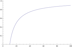
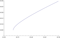
Figure 1: Numerical results for $C$ as a function of $r$. $C(r)$ is non-zero (positive) at $r=a$ and well defined only for $r\geq a$. Left: $C(r)$ vs. $r$ from $r=a$ to $r\gg a$. Right: $C(r)$ vs. $r$ for a small neighborhood of $r=a$. Here, $a_{0}=10$ and $\alpha=2$.

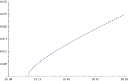
Figure 2: Numerical results for $F$ as a function of $r$. $F(r)$ vanishes at $r=a$. Left: $F(r)$ vs. $r$ from $r=a$ to $r\gg a$. Right: $F(r)$ in a small neighborhood of $r=a$.

In support of our analysis above, we have solved $C(r)$ and $F(r)$ numerically from eq.(66) and (67), as shown in Fig. 1 for $C(r)$ and Fig. 2 for $F(r)$. The diagrams for $C(r)$ and $F(r)$ are only plotted for $r\geq a$ simply because $r=a$ is a minimum of $r$. The numerical simulation for $C$ as a function of $r_{*}$ is shown in Fig. 3, and the solution can be extended indefinitely in both limits $r_{*}\to\pm\infty$. The numerical solution of $r$ as a function of $r_{*}$ is displayed in Fig. 4, showing that $r$ has a local minimum.

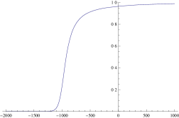
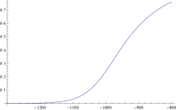
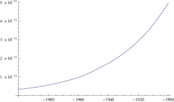
Figure 3: Numerical results for $C$ as a function of $r_{*}$. Top: $C(r_{*})$ vs. $r_{*}$ from $r_{*}\ll a_{*}$ to $r_{*}\gg a_{*}$. Left: $C(r_{*})$ vs. $r_{*}$ in a small neighborhood of $r_{*}=a_{*}$. Right: $C(r_{*})$ vs. $r_{*}$ for $r_{*}\ll a_{*}$.

Although the horizon is absent, i.e. $C(r)$ does not vanish at $r=a$, the value of $C(a)$ is indeed extremely small for a large Schwarzschild radius, of order ${\cal O}(\alpha/a^{2})$ (see (81)). The red-shift factor relating the time coordinate $t$ in the neighborhood of $r=a$ to the time coordinate $t$ at large $r$ is given by $c_{0}^{1/2}$. There is an even larger red-shift for $r<a$. As a result, everything close to or inside the Schwarzschild radius looks nearly frozen to a distant observer. For a large Schwarzschild radius, a real black hole with a horizon and a wormhole with a large red-shift factor is very hard to distinguish by observations at distance.

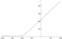
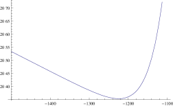
Figure 4: Numerical results for $r$ as a function of $r_{*}$. Left: $r$ vs. $r_{*}$ from $r_{*}\ll a_{*}$ to $r_{*}\gg a_{*}$. Right: $r$ vs. $r_{*}$ in a small neighborhood of $r=a$. The slope is very close to zero but finite for $r_{*}<a_{*}$.

The conventional expectation of the Boulware vacuum is that the vacuum energy-momentum tensor would diverge at the horizon if the radius of the star is smaller than the Schwarzschild radius. But this expectation is based on the calculation that has neglected back reaction. According to our non-perturbative solution of $C$ and $F$, in the small neighborhood (80) of $r=a$,

$$\langle T^{(2)}_{uu}\rangle \simeq-\frac{N}{48\pi}\frac{c_{0}}{\alpha}\sim\mathcal{O}(1/a^{2})\ ,$$ (86)

$$\langle T^{(2)}_{uv}\rangle \simeq 0\ ,$$ (87)

and $\langle T^{(2)}_{vv}\rangle$ is the same as $\langle T^{(2)}_{uu}\rangle$. According to (81), $\langle T^{(2)}_{uu}\rangle$ is of the same order ${\cal O}(1/a^{2})$ as its counterpart (30) before back reaction is taken into consideration. $\langle T^{(2)}_{uv}\rangle$ vanishes as its counterpart does at $r=a_{0}$. Since $C(a)=c_{0}$ is very small (81), the energy-momentum tensor at $r=a$ in a local frame is highly blue shifted. But it is only of order ${\cal O}(\alpha^{-1}a^{-2}))$, much smaller than the Planck energy density $\alpha^{-2}$. This invalidates the conventional expectation that the energy-momentum tensor diverges at the horizon for the Boulware vacuum.

Since this is no longer a classical vacuum solution, the Einstein tensor becomes non-zero at $r=a$. In the small neighborhood (80) around $r=a$, the Einstein tensor is of order

$$G^{u}{}_{v}\sim G^{v}{}_{u}\sim{\cal O}(1/a^{2})\ ,\qquad G^{u}{}_{u}\sim G^{v}{}_{v}\sim 0\ .$$ (88)

The order of magnitude of $G^{u}{}_{v}$ (${\cal O}(1/a^{2})$) is small for large $a$, so that it is consistent to use the low-energy effective description of gravity (Einstein’s equations).

Notice that the disappearance of horizon is not a fine-tuned result. It is insensitive to many details in eq.(67), but only relies on the fact that the dominant terms are $\rho^{\prime\prime}$ and $\rho^{\prime}{}^{3}$. The appearance of a wormhole-like geometry demands that the ratio of the coefficients of these two terms be positive, but in Sec. 4.1 below, we will see that there is still no horizon if the ratio is negative, although the geometry would be different.

We have only considered the local structure at the Schwarzschild radius, where the near-horizon geometry is replaced by a wormhole-like structure. It is possible that there is a horizon or singularity deep down the throat. In fact, the result about a wormhole-like structure (which was called a “bounce”) was first discovered in Ref.[35] via numerical analysis. In addition they mentioned the possibility of a curvature singularity deep down the throat in the limit $r\to\infty$ (but within finite affine distance) where $C$ goes to zero [35]. The results of their numerical analysis are completely consistent with the discussion in this section, although our focus is on the near-horizon geometry. Note that the singularity deep down the throat in the vacuum solution is relevant only if the surface of the star does not exist until $r\to\infty$ and the mass of the star is localized at the singularity in $r\to\infty$. However, in a more realistic scenario, the surface of the star has a finite area $(r<\infty)$ and so the singularity at $r=\infty$ for the vacuum solution is irrelevant. The singularity is hence not a robust feature of the wormhole-like geometry.

3.5 Hartle-Hawking Vacuum

For a more general background, the energy-momentum tensor (23) has the additional terms $\hat{T}_{\mu\nu}$. For stationary solutions, these terms are constants so that

$$\langle T^{(2)}_{uu}\rangle=\langle T^{(2)}_{vv}\rangle=\frac{F(r)}{192\pi C^{2}(r)}[-3F(r){C^{\prime}}^{2}(r)+2C(r)(F^{\prime}(r)C^{\prime}(r)+F(r)C^{\prime\prime}(r))]+\frac{b}{48\pi\alpha}$$ (89)

for some constant $b$. Then the Einstein equations become

$$FC^{\prime}-F^{\prime}C-\frac{\alpha}{2}\frac{1}{r}(F^{\prime}C^{\prime}+FC^{\prime\prime})+\frac{3\alpha}{4}\frac{1}{Cr}F{C^{\prime}}^{2}-b\frac{C}{rF} =0\ ,$$ (90)

$$\frac{C^{2}}{Fr}-\frac{FC}{r}-F^{\prime}C-\frac{\alpha}{2}\frac{1}{r}(F^{\prime}C^{\prime}+FC^{\prime\prime})+\frac{\alpha}{2}\frac{1}{Cr}F{C^{\prime}}^{2} =0\ .$$ (91)

Since the weak energy condition should not be violated in the asymptotic Minkowski space at $r\rightarrow\infty$, we shall assume that $b\geq 0$. This leads to a positive outgoing energy flux at spatial infinity as well as an ingoing energy flux of the same magnitude. The conventional interpretation for this boundary condition is that the Hawking radiation from the black hole is balanced by an ingoing energy flux from a thermal background at the Hawking temperature, and the corresponding quantum state is called the Hartle-Hawking vacuum.

Due to the energy flux at spatial infinity, the asymptotic geometry at $r\rightarrow\infty$ is no longer Minkowskian. Instead,

$$C(r)\simeq 2b\log(r)+2b\log\log(r)+\cdots$$ (92)

in the limit $r\rightarrow\infty$. However, for small $b$, this approximation only applies at extremely large $r$ ($r$ of order ${\cal O}(e^{1/b})$ or larger). If we restrict ourselves to a much smaller neighborhood that is still much larger than the Schwarzschild radius, we can still think of the Schwarzschild metric as the approximate solution in the large $r$ limit.

Let us now study the asymptotic behavior of the solution to the Einstein equation as we zoom into a small neighborhood of the Schwarzschild radius. From the Einstein equations, we obtain

$$F=2C\sqrt{\frac{C+b}{4C^{2}+4rCC^{\prime}+\alpha C^{\prime\,2}}}\ .$$ (93)

Plugging it back to the Einstein equation, we find

$$0 =C^{\prime}(r)^{2}\left[\alpha rC^{\prime}(r)-4b\left(r^{2}-\alpha\right)\right]+4C(r)^{2}\left[\left(r^{2}-\alpha\right)C^{\prime\prime}(r)+2rC^{\prime}(r)-2b\right]$$

$$\qquad+C(r)\left[4b\left(r^{2}-\alpha\right)C^{\prime\prime}(r)-4brC^{\prime}(r)+6\alpha C^{\prime}(r)^{2}\right]\ .$$ (94)

The perturbative expansions

$$C(r) =C_{0}(r)+\alpha C_{1}(r)+\cdots\ ,$$ (95)

$$b =\alpha b_{1}+\cdots\ ,$$ (96)

give the solution for (94) as

$$C_{0}(r) =1-\frac{a_{0}}{r}\ ,$$ (97)

$$C_{1}(r) =-\frac{(2r-a_{0})^{2}}{8a_{0}r^{3}}-\frac{c_{1}+a_{0}b_{1}}{r}+\frac{2r-3a_{0}}{4a_{0}^{2}r}\left[\log r-(1-4a_{0}^{2}b_{1})\log(r-a_{0})\right]\ ,$$ (98)

where the terms inversely proportional to $r$ in $C_{1}(r)$ can be absorbed in a shift of the Schwarzschild radius $a_{0}$ in $C_{0}(r)$ by an order-$\alpha$ correction. The next-to-leading order term $C_{1}(r)$ diverges except for

$$b_{1}=\frac{1}{4a_{0}^{2}}\ .$$ (99)

This is the condition on the energy flux at spatial infinities for the Hartle-Hawking vacuum.

In addition to the perturbative approach via expansions in Newton’s constant, we shall also study the near-horizon geometry of the Hartle-Hawking vacuum that is non-perturbative in $\alpha$ in the limit $r\rightarrow a$. If there is a Killing horizon, i.e., $C$ has a zero at $r=a$, we assume that

$$C(r)=c_{0}(r-a)^{n}+\cdots$$ (100)

for some constant $n>0$, and then eq.(94) can be expanded as

$$0=(r-a)^{2n-2}\left[4(a^{2}-\alpha)bc_{0}^{2}n+\mathcal{O}(r-a)\right]-(r-a)^{3n-3}\left(\alpha ac_{0}^{3}n^{3}+\mathcal{O}(r-a)\right)\ .$$ (101)

To satisfy this equation, the term of order $\mathcal{O}((r-a)^{2n-2})$ and that of order $\mathcal{O}((r-a)^{3n-3})$ must cancel. Hence

$$n=1\ ,$$ (102)

and the equation becomes

$$0=c_{0}^{2}(4\alpha b-4a^{2}b+\alpha ac_{0})+\mathcal{O}(r-a)\ .$$ (103)

Therefore, $C(r)$ has a zero only if

$$b=\frac{c_{0}\alpha a}{4(a^{2}-\alpha)}\ ,$$ (104)

which is consistent with the perturbative result (99). This is the condition for the existence of horizon. In this case, $F$ is given by

$$F=2\sqrt{\frac{b}{\alpha}}\,(r-a)+\mathcal{O}((r-a)^{2})\ .$$ (105)

As the classical Schwarzschild solution, the near-horizon geometry for the Hartle-Hawking vacuum is given by the Rindler space.

Note that the condition (104) requires a fine-tunning of the value of $b$. Hence it establishes a connection between the existence of horizon and the magnitude of Hawking radiation.

Next, consider the case when there is no horizon, that is, $C(r)$ does not go to zero, although $\rho^{\prime}(r)$ diverges at some point $r=a$. In the limit $r\rightarrow a$, we can expand $C(r)$ as

$$C(r)=c_{0}+c_{1}(r-a)^{n}+\cdots\ ,$$ (106)

Then, the Einstein equation is expanded as

$$0 =8bc_{0}^{2}+(r-a)^{n-2}\left[4(a^{2}-\alpha)(c_{0}+b)c_{0}c_{1}n(n-1)+\mathcal{O}(r-a)\right]+\mathcal{O}((r-a)^{2n-2})$$

$$\qquad-(r-a)^{3n-3}\left(\alpha ac_{1}^{3}n^{3}+\mathcal{O}(r-a)\right)\ .$$ (107)

The assumption that $\rho^{\prime}(r)$ diverges at $r=a$ implies that $n<1$, hence the term of order $\mathcal{O}((r-a)^{n-2})$ and the term of order $\mathcal{O}((r-a)^{3n-3})$ must cancel each other, so we need

$$n=1/2\ .$$ (108)

The equation above is expanded as

$$0=(r-a)^{-3/2}\left[\frac{1}{8}\alpha ac_{1}^{3}-(a^{2}-\alpha)(c_{0}+b)c_{0}c_{1}\right]+\mathcal{O}\left(\frac{1}{r-a}\right)\ .$$ (109)

It determines $c_{1}$ as

$$c_{1}=\sqrt{\frac{8(a^{2}-\alpha)(c_{0}+b)c_{0}}{\alpha a}}\ .$$ (110)

The ratio $c_{0}/c_{1}$ restricts the range of validity for the approximation (106) to the region (80). One can then estimate $c_{0}$ as

$$c_{0}\leq{\cal O}\left(\frac{\alpha}{a^{2}}\right)$$ (111)

by matching $C(r)$ (106) around the point $r-a\sim{\cal O}(\alpha/a)$ with the Schwarzschild solution.

We use eq.(93) to compute $F$ and find

$$F=\sqrt{\frac{2ac_{0}}{a^{2}-\alpha}}\,\sqrt{r-a}+\mathcal{O}(r-a)$$ (112)

in the limit $r\rightarrow a$. As we have seen in the previous section, this solution describes the wormhole-like geometry in a small neighborhood of $r=a$.

To summarize this subsection, the horizon is possible only if $b$ is fine-tuned to the value given by eq.(104). In general, there is a wormhole solution for arbitrary non-negative $b$, including the case (104). In the wormhole-like solution, $\langle T^{(4)}_{uu}\rangle$ is non-zero and negative at $r=a$:

$$\langle T^{(4)}_{uu}(a)\rangle=-\frac{c_{0}}{2\alpha(a^{2}-\alpha)}\ .$$ (113)

Its order of magnitude is ${\cal O}(1/a^{4})$. When there is a horizon, $\langle T^{(4)}_{uu}\rangle$ vanishes at the horizon.

4 4D Scalars as Dilaton-Coupled 2D Scalars

In this section, we consider the 2-dimensional dilaton-coupled scalar (4), which is the dimensionally reduced 4-dimensional scalar with spherical symmetry. Due to the coupling with dilaton, the Weyl anomaly acquires additional terms as [33]

$$\langle T^{(2)\,\mu}{}_{\mu}\rangle=\frac{1}{24\pi}\left[R^{(2)}-6(\partial\phi)^{2}+6\nabla^{2}\phi\right]\ ,$$ (114)

where $\mu$ is a 2-dimensional Lorentz index.

We shall consider the back reaction of the energy-momentum tensor with this anomaly, and assume that there is no incoming or outgoing flux at spatial infinity. However, the 4-dimensional conservation law (11) and the Weyl anomaly (114) do not uniquely fix the energy-momentum tensor, leaving one degree of freedom unfixed. One needs to impose an additional condition on the vacuum energy-momentum tensor, corresponding to the choice of a quantum state. We shall consider three possible choices: (1) $\langle T^{(4)}_{\theta\theta}\rangle=\langle T^{(4)}_{\phi\phi}\rangle=0$ (Sec. 4.1), (2) $\langle T^{(4)}_{uu}\rangle=\langle T^{(4)}_{vv}\rangle=0$ (Sec. 4.2), and (3) the energy-momentum tensor according to Ref.[34] (Sec. 4.3).

4.1 Case I: $\langle T_{\theta\theta}^{(4)}\rangle=\langle T_{\phi\phi}^{(4)}\rangle=0$

We first consider the vacuum state in which the energy-momentum tensor satisfies the 2-dimensional conservation law (13), as well as the 4-dimensional one (11). This implies that the angular components of the energy-momentum tensor vanish identically,

$$\langle T^{(4)}_{\theta\theta}\rangle=\langle T^{(4)}_{\phi\phi}\rangle=0\ ,$$ (115)

as in the previous section.

In this case, the angular components of the Einstein equation, or equivalently, the equation of motion for the dilaton $\phi$ is

$$2\nabla^{2}\phi-2(\partial\phi)^{2}+R^{(2)}=0\ .$$ (116)

The Weyl anomaly (114) is thus simplified to

$$\langle T^{(2)\,\mu}{}_{\mu}\rangle=-\frac{1}{12\pi}R^{(2)}\ ,$$ (117)

which takes the same form as (16) but with an additional overall factor of $-2$.

The energy-momentum tensor is now completely fixed by the conservation law. It has the same forms as that of the toy model, i.e. (20)–(22), but with additional overall factors of $-2$. The extra factor of $-2$ can be absorbed in a redefinition of the parameter $\alpha$:

$$\alpha=-\frac{\kappa N}{12\pi}\ ,$$ (118)

which is now negative, and then the equations in the previous section, e.g. (66)–(68), remain formally the same.

Because of the change in sign of the parameter $\alpha$, we expect that the energy-momentum tensor outside the star be positive, and the behavior of the solution near the Schwarzschild radius can be quite different from the toy model in Sec. 3. In order for the horizon or the wormhole-like geometry to appear at $r=a$, we need

$$\rho^{\prime}(r) \to\infty\ ,$$ (119)

in the limit of $r\to a$, which implies that

$$\rho^{\prime\prime}(r) \to-\infty$$ (120)

in the limit. However, eqs.(119) and (120) are inconsistent with the Einstein equation (67). Eq.(119) implies that eq.(73) holds when $r$ is sufficiently close to $a$, so that eq.(67) can be approximated by (74). Yet eq.(74) implies that $\rho^{\prime\prime}$ must be positive for $\alpha<0$ and $r^{2}>\alpha$.

The condition (119) can therefore never be satisfied. As we gradually decrease $r$, the value of $\rho^{\prime}$ increases only when $r$ is sufficiently large. But the value of $\rho^{\prime}$ starts to decrease with $r$ before it is large enough to satisfy the condition (73). It is therefore inconsistent to assume the existence of a horizon or a wormhole for the quantum state satisfying the condition (115).

In support of our analysis, the numerical solutions to the Einstein equation are shown in Fig.5 for $C(r)$ and Fig.6 for $F(r)$. As $F(r)$ is always positive, the value of $r$ has no local minimum. In this sense it is not like a wormhole, but only a throat that gets narrower and narrower as one falls towards the center. There is no horizon either as $C(r)$ is always positive. Nevertheless, $C(r)$ is extremely small for $r\sim a$ and $r<a$, so there is a huge blue-shift for a distant observer. Everything close to or inside the Schwarzschild radius appears to be nearly frozen, and it is hard to be distinguished from a real black hole from the viewpoint of a distant observer.

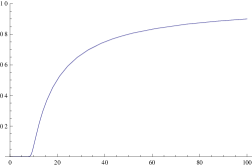
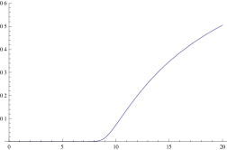
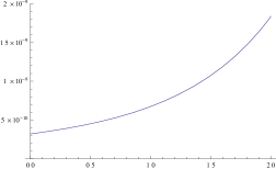
Figure 5: Numerical results for $C(r)$. Top: $C(r)$ vs. $r$ from $r=0$ to $r\gg a$. Left: $C(r)$ vs. $r$ in a small neighborhod near $r=a$. Right: $C(r)$ vs. $r$ near $r=0$. $C(r)$ is always positive.

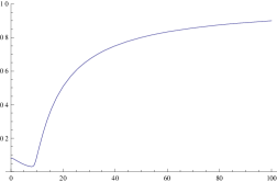
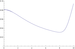
Figure 6: Numerical results for $F(r)$. Left: $F(r)$ vs. $r$ from $r=0$ to $r\gg a$. Right: $F(r)$ vs. $r$ in a neighborhood of $r=a$. $F(r)$ is always positive.

4.2 Case II : $\langle T^{(4)}_{uu}\rangle=\langle T^{(4)}_{vv}\rangle=0$

As another example, we impose the condition

$$\langle T^{(4)}_{uu}\rangle=\langle T^{(4)}_{vv}\rangle=0$$ (121)

by hand and investigate the corresponding geometry. The 4-dimensional conservation law implies

$$\partial_{r}\left(\frac{\langle T^{(2)}_{uv}\rangle}{C}\right)-2r\langle T^{(4)\theta}{}_{\theta}\rangle=0\ ,$$ (122)

which determines $\langle T^{(4)\theta}{}_{\theta}\rangle$ in terms of $\langle T^{(2)}_{uv}\rangle$.

In this case, the equations of motion are given by

$$0 =FC^{\prime}-F^{\prime}C\ ,$$ (123)

$$0 =rC^{2}\left(C+F^{2}+rFF^{\prime}\right)+\alpha F\left(-6C^{2}F^{\prime}+rCC^{\prime}F^{\prime}+rFC^{\prime\,2}-rFCC^{\prime\prime}\right)\ .$$ (124)

We first solve these equations for $F(r)$ and obtain

$$F(r)=\frac{C(r)}{\sqrt{C(r)+rC^{\prime}(r)+6\alpha r^{-1}C^{\prime}(r)+\alpha C^{\prime\prime}(r)}}\ .$$ (125)

Plugging this back into (123) or (124), we obtain the differential equation for $C(r)$:

$$\alpha r^{2}C^{\prime\prime\prime}(r)+(r^{3}+6\alpha r)C^{\prime\prime}(r)+(2r^{2}+6\alpha)C^{\prime}(r)=0\ .$$ (126)

The solution of this equation is given by

$$C(r)=1-\frac{1}{r^{5}}\left[\left(r^{4}-2\alpha r^{2}+3\alpha^{2}\right)\left(c_{1}-c_{2}\sqrt{\pi}\,\mathrm{erfc}((2\alpha)^{-1/2}r)\right)+\sqrt{2\alpha}\,\left(r^{2}-3\alpha\right)e^{-\frac{r^{2}}{2\alpha}}\right]\ ,$$ (127)

where erfc is the complementary error function, which is defined by

$$\mathrm{erfc}(x)=\frac{2}{\sqrt{\pi}}\int_{x}^{\infty}e^{-t^{2}}dt\ ,$$ (128)

and $c_{1}$ and $c_{2}$ are integration constants. We have chosen the other integration constant such that $C(r)\to 1$ in the limit $r\to\infty$.

The solution (127) has zeros for suitable choices of the parameters $c_{1}$ and $c_{2}$. For example, for $c_{2}=0$, the radius of the horizon is given by a solution of

$$(15\alpha^{2}-6\alpha+1)r^{5}-c_{1}r^{4}+2\alpha c_{1}r^{2}-3\alpha^{2}c_{1}=0\ .$$ (129)

Since $C(r)$ behaves in the limit $r\to\infty$ as

$$C(r)\simeq 1-\frac{c_{1}}{r}+\cdots+\frac{16\alpha^{5/2}c_{2}}{r^{6}}e^{-\frac{r^{2}}{2\alpha}}+\cdots\ ,$$ (130)

the constant $c_{1}$ is related to the mass of the black hole. The other constant $c_{2}$ specifies the quantum correction, as it is suppressed in the limit $\alpha\to 0$, and hence it is not related to the classical configuration, but a parameter for different vacua.

4.3 Case III 

In this subsection, the components $\langle T_{uu}^{(2)}\rangle$ and $\langle T_{vv}^{(2)}\rangle$ of the energy-momentum tensor for the 2D dilaton-coupled scalar field are calculated using the formula derived in Ref.[34]:

$$\langle T_{uu}^{(2)}\rangle =-\frac{1}{12\pi}\left(\partial_{u}\rho\partial_{u}\rho-\partial^{2}_{u}\rho\right)+\frac{1}{2\pi}\left(\partial_{u}\rho\partial_{u}\phi+\rho(\partial_{u}\phi)^{2}\right)\ ,$$ (131)

$$\langle T_{vv}^{(2)}\rangle =-\frac{1}{12\pi}\left(\partial_{v}\rho\partial_{v}\rho-\partial^{2}_{v}\rho\right)+\frac{1}{2\pi}\left(\partial_{v}\rho\partial_{v}\phi+\rho(\partial_{v}\phi)^{2}\right)\ ,$$ (132)

where $\rho$ is defined by (68) and $\phi$ by

$$\phi=-\log(r/\mu)\ .$$ (133)

The trace anomaly (114) is expressed in terms of $\phi$ and $\rho$ as

$$\langle T_{uv}^{(2)}\rangle=-\frac{1}{12\pi}\left(\partial_{u}\partial_{v}\rho+3\partial_{u}\phi\partial_{v}\phi-3\partial_{u}\partial_{v}\phi\right)\ .$$ (134)

The angular components of the energy-momentum tensor is now non-zero and is determined through the 4-dimensional conservation law (12) by the rest of the energy-momentum tensor (131)-(134).

The energy-momentum tensor (131)-(134) can be rewritten in terms of $\rho$ and $F$ as

$$\langle T^{(2)}_{uu}\rangle =\frac{F(r)}{192\pi}\left[F^{\prime}(r)\rho^{\prime}(r)+F(r)\left(-\rho^{\prime\,2}(r)+\rho^{\prime\prime}(r)\right)+\frac{6}{r^{2}}F(r)\left(\rho(r)-r\rho^{\prime}(r)\right)\right]\ ,$$ (135)

$$\langle T^{(2)}_{vv}\rangle =\frac{F(r)}{192\pi}\left[F^{\prime}(r)\rho^{\prime}(r)+F(r)\left(-\rho^{\prime\,2}(r)+\rho^{\prime\prime}(r)\right)+\frac{6}{r^{2}}F(r)\left(\rho(r)-r\rho^{\prime}(r)\right)\right]\ ,$$ (136)

$$\langle T^{(2)}_{uv}\rangle =\frac{F(r)}{192\pi}\left[F^{\prime}(r)\rho^{\prime}(r)+F(r)\rho^{\prime\prime}(r)+\frac{3F^{\prime}(r)}{r}\right]\ .$$ (137)

By using these expressions together with those for the Einstein tensor (47)-(49), the semi-classical Einstein equation (10) gives the following differential equations:

$$0 =-r^{2}F^{\prime}(r)\left(2\alpha\rho^{\prime}(r)+r\right)$$

$$\qquad-2F(r)\left[\alpha r^{2}\rho^{\prime\prime}(r)-\alpha r^{2}\rho^{\prime\,2}(r)-r(r^{2}-6\alpha)\rho^{\prime}(r)+6\alpha\rho(r)\right]\ ,$$ (138)

$$0 =e^{2\rho(r)}-F(r)F^{\prime}(r)\left(2\alpha r\rho^{\prime}(r)+r^{2}+6\alpha\right)-F^{2}(r)\left(2\alpha r\rho^{\prime\prime}(r)+r\right)\ .$$ (139)

From these differential equations, we can easily solve $F(r)$ as

$$F(r)=e^{\rho(r)}r^{3/2}\sqrt{\frac{2\alpha\rho^{\prime}(r)+r}{D(r)}}\ ,$$ (140)

where the function $D(r)$ is

$$D(r) =r^{4}-12\alpha^{2}r^{2}\rho^{\prime\prime}(r)-12\alpha\rho(r)\left(2\alpha r\rho^{\prime}(r)+r^{2}+6\alpha\right)$$

$$\qquad+2\rho^{\prime}(r)\left[\alpha r^{2}\rho^{\prime}(r)\left(2\alpha r\rho^{\prime}(r)+3(r^{2}+6\alpha)\right)+r(r^{2}+4\alpha)(r^{2}+9\alpha)\right]\ .$$ (141)

Plugging (140) back into (138) or (139), we obtain the differential equation for $\rho(r)$:

$$0 =-24\alpha^{2}r^{2}\rho(r)\rho^{\prime\prime}(r)\left(15\alpha+r^{2}+2\alpha r\rho^{\prime}(r)\right)-144\alpha^{2}r^{2}\rho(r)$$

$$\quad+12\alpha r\rho(r)\rho^{\prime}(r)\left[4\alpha r\rho^{\prime}(r)\left(14\alpha+2r^{2}+\alpha r\rho^{\prime}(r)\right)+3r^{4}+40\alpha r^{2}+126\alpha^{2}\right]$$

$$\quad+2\alpha r^{3}\left(186\alpha^{2}+3r^{4}+56\alpha r^{2}\right)\rho^{\prime}(r)^{3}+4\alpha^{2}r^{4}\left(12\alpha+r^{2}\right)\rho^{\prime}(r)^{4}$$

$$\quad+2r^{2}\rho^{\prime}(r)^{2}\left(324\alpha^{3}+r^{6}+27\alpha r^{4}-18\alpha^{3}r^{2}\rho^{\prime\prime}(r)+162\alpha^{2}r^{2}\right)$$

$$\quad-6\alpha^{2}r^{5}\rho^{(3)}(r)+r^{4}\rho^{\prime\prime}(r)\left(48\alpha^{2}+r^{4}+10\alpha r^{2}+36\alpha^{3}\rho^{\prime\prime}(r)\right)$$

$$\quad+2r^{3}\rho^{\prime}(r)\left(-72\alpha^{2}+r^{4}-3\alpha r^{2}+\alpha\left(-138\alpha^{2}+r^{4}-14\alpha r^{2}\right)\rho^{\prime\prime}(r)-6\alpha^{3}r\rho^{(3)}(r)\right)\ .$$ (142)

If there is a Killing horizon at $r=a$, we must have $\rho\to-\infty$ as $r\to a$. Then $\rho$ would behave around $r=a$ as either

$$\rho(r)=\rho_{0}\log(r-a)+\cdots\ ,$$ (143)

or

$$\rho(r)=\frac{1}{2}\log c_{0}+\rho_{0}(r-a)^{n}+\cdots$$ (144)

with $n<0$.

Assuming eq.(143), which includes the case of the Schwarzschild solution, the Einstein equation (142) can be expanded as

$$0=4\alpha^{2}a^{4}\rho_{0}^{2}\left(a^{2}\rho_{0}^{2}+12\alpha\rho_{0}^{2}+9\alpha\rho_{0}+3\alpha\right)\frac{1}{(r-a)^{4}}+\mathcal{O}\left(\frac{1}{(r-a)^{3}}\right)\ ,$$ (145)

and we can solve $\rho_{0}$ as

$$\rho_{0}=\frac{1}{2a^{2}+24\alpha}\left(-9\alpha\pm\sqrt{-12\alpha a^{2}-63\alpha^{2}}\right)\ ,$$ (146)

which is never real since $a^{2}\gg\alpha$. Therefore, $\rho$ can never behave as (143) near $r=a$.

For the other option (144), the Einstein equation (142) is expanded as

$$0 =36\alpha^{2}\log c_{0}\left[2a^{2}+(a^{2}+6\alpha)\log c_{0}\right]+\mathcal{O}(r-a)$$

$$\quad+(r-a)^{n-3}\left[-6\alpha^{2}a^{5}n(n-1)(n-2)\rho_{0}+\mathcal{O}(r-a)\right]$$

$$\quad+(r-a)^{2n-4}\left[12\alpha^{3}a^{4}n^{2}(n-1)(2n-1)\rho_{0}^{2}+\mathcal{O}(r-a)\right]$$

$$\quad-(r-a)^{3n-4}\left[36\alpha^{3}a^{4}n^{3}(n-1)\rho_{0}^{3}+\mathcal{O}(r-a)\right]$$

$$\quad+(r-a)^{4n-4}\left[4\alpha^{2}a^{4}(a^{2}+12\alpha)n^{4}\rho_{0}^{4}+\mathcal{O}(r-a)\right]+\mathcal{O}(1)\ .$$ (147)

In order for the leading order terms to cancel, we need

$$n=\frac{1}{2}\ .$$ (148)

Then, $C(r)$ behaves near $r=a$ as

$$C(r)\simeq c_{0}e^{2\rho_{0}\sqrt{r-a}}\ .$$ (149)

The coefficient $\rho_{0}$ can be fixed from the leading order term of the expansion of (142) around $r=a$,

$$0=\frac{9}{4}\alpha^{2}a^{4}\rho_{0}(\alpha\rho_{0}^{2}-a)(r-a)^{-5/2}+\mathcal{O}((r-a)^{-2})\ ,$$ (150)

to be

$$\rho_{0}=\sqrt{\frac{a}{\alpha}}\ .$$ (151)

Using (140) with (149), we find

$$F(r)\simeq\sqrt{\frac{2c_{0}a(r-a)}{\alpha(a\rho_{0}^{2}+6)}}$$ (152)

in the limit $r\to a$. Since $C(r)$ is non-zero and $F(r)$ behaves as $\mathcal{O}(\sqrt{r-a})$ near $r=a$, the metric in the limit $r\to a$ is approximately given by that of the wormhole as in the case of Sec. 3.

The back reaction of vacuum energy due to dilaton-coupled 2-dimensional scalar has been studied previously in Ref. [35], which announced the absence of horizon and the existence of a “turning point” (i.e. $F(a)=0$) using numerical analysis, in agreement with our results of analytic arguments. They also claimed that there is a divergence of $F$ beyond the turning point in their numerical analysis. Such a singularity exists only if the surface of the star is sufficiently far away from the point $r=a$ so that the vacuum solution still applies to the neighborhood of the singularity. As our focus is on the local geometry that replaces the near-horizon region, a singularity further down the throat is not of our concern. (See the discussion at the end of Sec. 3.4.)

Incidentally, let us prove analytically that there is no singularity which is associated to the pole of $F(r)$. As we have discussed above, $C(r)$ does not have divergence or zero at finite and non-zero $r$. If there is a curvature singularity but $C(r)$ is regular there, $F(r)$ must diverge at the singularity. It was also proposed in Ref. [35] by using numerical analyses that the singularity occurs at a point $r=r_{M}$ where $\rho$ is finite and $F$ diverges as $F(r)\propto(r_{M}-r)^{-1/2}$ in the limit $r\rightarrow r_{M}$, (See eq.(103) in Ref.[35].) for the semi-classical Einstein equations (eqs.(30)-(32) in Ref.[35]) which is identical to (138)-(139) in this paper. However, the singularity of this sort is incompatible with the semi-classical Einstein equations (138)-(139), as we now prove below. First of all, according to (152), $F(r)$ must be finite if $\rho^{\prime}$ diverges. This implies that $\rho^{\prime}(r_{M})$ must be finite if $F(r)$ diverges as

$$F(r)\propto(r_{M}-r)^{n}\$$ (153)

for some negative $n$ ($n=-1/2$ in Ref.[35]). The leading order terms in the Einstein equations (138) and (139) are then

$$0 =-n(2\alpha\rho^{\prime}(r_{M})+r_{M})r_{M}^{2}(r_{M}-r)^{n-1}\ ,$$ (154)

$$0 =-n(2\alpha r_{M}\rho^{\prime}(r_{M})+r_{M}^{2}+6\alpha)(r_{M}-r)^{2n-1}\ .$$ (155)

Hence we see that the two Einstein equations are inconsistent with their ansatz of the singularity. Therefore, the singularity can exist only in the limit $r\to\infty$, although it can be in a finite affine distance from finite $r$.

5 Energy-Momentum Tensor and Near-Horizon Geometry

In Secs. 3 and 4, we considered different models of the vacuum energy-momentum tensor, which is always found to be regular at the horizon (in a local orthonormal frame) when the back reaction is taken into account. Our opinion is that a reasonable model for the vacuum energy-momentum tensor should prevent divergence in local orthonormal frames by itself at least at the macroscopic scale. We also found that sometimes the existence of horizon demands fine-tunning, and it can be easily deformed into a wormhole-like geometry without horizon by a small modification of the energy-momentum tensor within a tiny range of space. Our observation is that horizons are extremely sensitive to tiny changes in the energy-momentum tensor at the horizon. In this section, we zoom into the tiny space around the horizon (or the wormhole-like space) and explore the connection between its geometry and the energy-momentum tensor, without specifying any detail about the physical laws behind the vacuum energy-momentum tensor.

We consider the (semi-classical) Einstein equations for 4-dimensional static, spherically symmetric geometries with an arbitrary energy-momentum tensor. According to eqs.(47)-(50), the Einstein equations are

$$G_{uu} =\frac{1}{2C(r)r}\left[F^{2}C^{\prime}(r)-\frac{1}{2}C(r)(F^{2})^{\prime}(r)\right]=\kappa T_{uu}\ ,$$ (156)

$$G_{vv} =\frac{1}{2C(r)r}\left[F^{2}C^{\prime}(r)-\frac{1}{2}C(r)(F^{2})^{\prime}(r)\right]=\kappa T_{vv}\ ,$$ (157)

$$G_{uv} =\frac{1}{2r^{2}}\left[C(r)-F^{2}-\frac{r}{2}(F^{2})^{\prime}(r)\right]=\kappa T_{uv}\ ,$$ (158)

$$G_{\theta\theta} =-\frac{r^{2}}{2C^{3}}\left[F^{2}C^{\prime\,2}-\frac{1}{2}(F^{2})^{\prime}CC^{\prime}-F^{2}CC^{\prime\prime}\right]+\frac{r}{2C}(F^{2})^{\prime}=\kappa T_{\theta\theta}\ .$$ (159)

Note that $F(r)$ appears only in the form of $F^{2}(r)$. In this section, we shall omit the superscript $(4)$ while all quantities are defined in the 4-dimensional theory. We will denote $\langle T^{(4)}_{\mu\nu}\rangle$ simply as $T_{\mu\nu}$.

For static and spherically symmetric configurations, the energy-momentum tensor $T_{\mu\nu}$ are functions which depend only on $r$. They allow us to solve the function $F$ as

$$F^{2}(r)=\frac{2\kappa r^{2}(T_{uu}(r)-T_{uv}(r))+C(r)}{2r\rho^{\prime}(r)+1}\ ,$$ (160)

where $\rho(r)$ is defined by

$$C(r)=e^{2\rho(r)}\ .$$ (161)

Incidentally, as results of the Einstein equations and spherical symmetry, we have

$$G_{\theta\theta} = -r^{2}R^{u}{}_{u}\ ,$$ (162)

$$R_{\theta\theta} = -r^{2}G^{u}{}_{u}\ .$$ (163)

The Einstein equations (156) – (159), together with the regularity of the energy-momentum tensor, will be our basis to establish the connection between the energy-momentum tensor and the existence of horizon.

5.1 Conditions for Horizon

For static configurations with spherical symmetry, the event horizon and the apparent horizon coincide with the Killing horizon. In this subsection, we consider the metric (33) with a Killing horizon at $r=a$, so

$$C(a)=0\ ,$$ (164)

which implies that

$$\rho\rightarrow-\infty\ ,\qquad\rho^{\prime}\rightarrow\infty$$ (165)

as $r\rightarrow a$. Assuming that $T_{uu}$ and $T_{uv}$ are finite, eq.(160) implies that $F(r)=0$ at the Killing horizon.

For solutions of the Einstein equation, the regularity of the geometry implies the regularity of the energy-momentum tensor. As $g^{uv}R_{uv}$ and $R_{\theta\theta}$ should both be regular for a regular space-time with spherical symmetry, eqs.(162) and (163) say that $g^{uv}T_{uv}$ and $T_{\theta\theta}$ should both be finite. Therefore, $T_{uv}$ must vanish at $r=a$ and it is convenient to express it in terms of $T^{u}{}_{u}=-2C^{-1}T_{uv}$, which should be regular but can be non-zero at $r=a$.

$F(r)$ (160) can thus be rewritten as

$$F^{2}(r)=\frac{2\kappa r^{2}T_{uu}(r)+C(r)(1+\kappa r^{2}T^{u}{}_{u}(r))}{2r\rho^{\prime}(r)+1}\ ,$$ (166)

where $T^{u}{}_{u}$ is regular at $r=a$. Since $C(a)=0$, we assume that $C$ can be expanded as

$$C(r)=c_{0}(r-a)^{n}+\cdots\ ,$$ (167)

in the limit $r\to a$ with $n>0$. Plugging (166) back to (156) or (158) and expand around $r=a$ by using (167), we obtain

$$0=(r-a)^{2n-2}\left[-2\kappa a^{2}c_{0}^{2}nT_{uu}(a)+\mathcal{O}(r-a)\right]+\mathcal{O}((r-a)^{3n-2})\ .$$ (168)

Therefore, the Einstein equation at the leading order implies that $T_{uu}$ (and $T_{vv}$) must vanish at the Killing horizon $r=a$.

The condition that $T_{uu}$ and $T_{vv}$ must vanish at the horizon can be understood as follows. Physically, the regularity of the energy-momentum tensor should be checked in a local orthonormal frame. The finiteness of $T_{uu}$ or $T_{vv}$ is not sufficient to ensure the regularity as the coordinates $(u,v)$ are singular at the horizon in the sense that $C(a)=0$ [36].

Let us now examine the regularity condition for the energy-momentum tensor at the horizon. At the future horizon ($du=0$), we should find another coordinate $\tilde{u}$ such that the metric is regular in the coordinate system $(\tilde{u},v)$. That is, in terms of the coordinates $(\tilde{u},v)$, the metric becomes

$$ds^{2}=-\widetilde{C}d\tilde{u}\,dv+r^{2}d\Omega^{2}\ ,$$ (169)

where

$$\widetilde{C}\equiv C\frac{du}{d\tilde{u}}\ ,$$ (170)

and we need $\widetilde{C}$ to be finite and non-zero at $r=a$ in order for $(\tilde{u},v)$ to be a regular local coordinate system at the horizon. Then, we have

$$\frac{du}{d\tilde{u}}\propto C^{-1}\to\infty$$ (171)

as $r\to a$, and therefore

$$T_{\tilde{u}\tilde{u}} =\left(\frac{du}{d\tilde{u}}\right)^{2}T_{uu}\ , T_{\tilde{u}{v}} =\frac{du}{d\tilde{u}}T_{uv}$$ (172)

would both diverge at $r=a$ unless

$$T_{uu}(a)=T_{uv}(a)=0\ .$$ (173)

Since $T_{vv}=T_{uu}$ for static configurations, we also have $T_{vv}=0$ at the horizon. To be more precise, $T_{uu}$, $T_{vv}$ and $T_{uv}$ must behave as

$$T_{uu} =\mathcal{O}(C^{2})\ , T_{vv} =\mathcal{O}(C^{2})\ , T_{uv} =\mathcal{O}(C)$$ (174)

as $r\to a$.

For static geometries, a coordinate system which covers only the intersection of the future and past horizons are sometimes used. In this case, we must transform both coordinates to new coordinates $(\tilde{u},\tilde{v})$ in order for the metric to be regular,

$$ds^{2}=-\widetilde{C}d\tilde{u}\,d\tilde{v}+r^{2}d\Omega^{2}\ ,$$ (175)

where

$$\widetilde{C}\equiv C\frac{du}{d\tilde{u}}\frac{dv}{d\tilde{v}}\ .$$ (176)

In order for $\widetilde{C}$ to be finite and non-zero at $r=a$, we need

$$\frac{du}{d\tilde{u}}\frac{dv}{d\tilde{v}}\propto C^{-1}\to\infty\ .$$ (177)

If we take $\tilde{u}$ and $\tilde{v}$ such that they are simply exchanged (up to sign) under the time reversal transformation, The energy-momentum tensor must behaves as

$$T_{uu} =\mathcal{O}(C)\ , T_{vv} =\mathcal{O}(C)\ , T_{uv} =\mathcal{O}(C)$$ (178)

in $r\to a$.

This simple mathematical result can have surprising implications because it says that it is possible for an arbitrarily small modification to the energy-momentum tensor at the horizon to kill the horizon. Conceptually, this explains why the horizon of the Schwarzschild solution disappears when we turn on the quantum correction to the vacuum energy-momentum tensor as we have shown in Secs. 3.4, 4.1 and 4.3. It also explains why one needs to fine-tune the additional energy flux in order to admit the existence of a horizon in Sec. 3.5.

5.2 Asymptotic Solutions in Near-Horizon Region

In this subsection, we shall examine more closely the relation between the energy-momentum tensor at the horizon and the near-horizon geometry for a series of near-horizon solutions.

For a generic quantum theory, the vacuum energy-momentum tensor is typically a polynomial of finite derivatives of the metric. Then, as we have shown in the examples in Secs.3 and 4, the Einstein equation in the limit $r\rightarrow a$ leads to a differential equation involving only the leading order terms:

$$(C^{(n_{1})})^{m_{1}}+a(C^{(n_{2})})^{m_{2}}(C^{(n_{2})})^{m_{3}}(\cdots)\simeq 0\ ,$$ (179)

where $(n_{1}),(n_{2}),(n_{3})$ are the order of derivatives with respect to $r$. If this equation admits an asymptotic solution as (167), $n$ must satisfy an algebraic equation of the form

$$m_{1}(n-n_{1})=m_{2}(n-n_{2})+m_{3}(n-n_{3})+\cdots\ .$$ (180)

which is always solved by a rational number

$$n=\frac{K}{M}\ ,\qquad(K,M\in\mathbb{Z}).$$ (181)

The subleading terms in $C(r)$ (167) in the limit $r\to a$ should be determined by the subleading terms in the Einstein equations. To be sure that the leading-order solution is part of a consistent solution, one needs a consistent expansion scheme for which higher and higher order terms in $C(r)$ can be solved order by order from the Einstein equations. In view of the Einstein equations (156)–(159), it is clear that a consistent ansatz for the expansion of $C(r)$ is

$$C(r)=(r-a)^{K/M}\left[c_{0}+c_{1}(r-a)^{1/M}+c_{2}(r-a)^{2/M}+\cdots\right]$$ (182)

for some integers $K\geq 0$ and $M\geq 1$. Eq.(160)) then implies that

$$F^{2}(r)=(r-a)^{K^{\prime}/M+1}\left[f_{0}^{2}+\tilde{f}_{1}(r-a)^{1/M}+\tilde{f}_{2}(r-a)^{2/M}+\cdots\right]$$ (183)

for a certain integer $K^{\prime}\geq 0$.

In the limit $r\to a$, the metric for $C(r)$ (182) and $F^{2}(r)$ (183) is

$$ds^{2} \simeq -c_{0}(r-a)^{K/M}dt^{2}+\frac{c_{0}}{f_{0}^{2}(r-a)^{(M+K^{\prime}-K)/M}}dr^{2}+a^{2}d\Omega^{2}$$ (184)

$$\simeq -c_{0}x^{2}dt^{2}+\frac{4M^{2}c_{0}}{K^{2}f_{0}^{2}}\frac{dx^{2}}{x^{2(K^{\prime}-M)/K}}+a^{2}d\Omega^{2}\ ,$$

where $r=a+x^{2M/K}$.

Assuming that there is no other length scale except $a$ and $\alpha$, the expansions (182) and (183) are expected to be valid when

$$0\leq r-a\ll\frac{\alpha}{a}\ .$$ (185)

A rough estimate of the values of $c_{0}$ and $f_{0}$ can be made by matching $C(r)$ and $F^{2}(r)$ at the leading order with the Schwarzschild solution for $r-a\sim{\cal O}(\alpha/a)$, if the solution is well approximated by the Schwarzschild metric at large $r$. We find

$$c_{0}\sim{\cal O}\left(\frac{\alpha^{1-K/M}}{a^{2-K/M}}\right)\ ,\qquad f_{0}^{2}\sim{\cal O}\left(\frac{\alpha^{1-K^{\prime}/M}}{a^{3-K^{\prime}/M}}\right)\ .$$ (186)

We now study the condition on the energy-momentum tensor in order for the horizon to exist. The energy-momentum tensor is determined by $C(r)$ (182) and $F^{2}(r)$ (183) through the Einstein equations as an expansion in powers of $(r-a)^{1/M}$:

$$\kappa T^{v}{}_{u}(r) = G^{v}_{u}=(r-a)^{(-K+K^{\prime})/M}\frac{(-2K+K^{\prime}+M)f_{0}^{2}}{2Mac_{0}}+\cdots\ ,$$ (187)

$$\kappa T^{u}{}_{u}(r) = G^{u}_{u}=-\frac{1}{a^{2}}+(r-a)^{(-K+K^{\prime})/M}\frac{(K^{\prime}+M)f_{0}^{2}}{2Mac_{0}}+\cdots\ ,$$ (188)

$$\kappa T_{\theta\theta}(r) = G_{\theta\theta}=-(r-a)^{(-M-K+K^{\prime})/M}\frac{K(M-K^{\prime})a^{2}f_{0}^{2}}{4M^{2}c_{0}}+\cdots\ .$$ (189)

Constraints should be imposed on the coefficients of the singular terms as $T^{v}{}_{u}(r)$, $T^{u}{}_{u}(r)$ and $T_{\theta\theta}(r)$ should all be regular at the horizon $r=a$, as we have argued above.

Depending on the values of $K,K^{\prime}$ and $M$, a solution can be classified into one of the following categories:

1. If $K>K^{\prime}$, in order for $T^{v}{}_{u}(a)$ and $T^{u}{}_{u}(a)$ to be finite, we need $K=0$, which implies that there is no horizon. This case will be considered in the next subsection.

2. If $K=K^{\prime}$, in order for $T_{\theta\theta}(a)$ to be finite, we need $M=K^{\prime}$ (and there are more constraints on the coefficients in the expansions of $C(r)$ (182) and $F^{2}(r)$ (183) if $M>1$). In such cases,

   $$\kappa T^{v}{}_{u}(a) = G^{v}{}_{u}=0\ ,$$ (190)

   $$\kappa T^{u}{}_{u}(a) = G^{u}{}_{u}=-\frac{1}{a^{2}}+\frac{f_{0}^{2}}{ac_{0}}>-\frac{1}{a^{2}}\ ,$$ (191)

   $$\kappa T_{\theta\theta}(a) = G_{\theta\theta}=\mbox{depends on $M$}\ ,$$ (192)

   $$ds^{2} \simeq -c_{0}(r-a)dt^{2}+\frac{c_{0}}{f_{0}^{2}(r-a)}dr^{2}+a^{2}d\Omega^{2}$$ (193)

   $$\simeq -c_{0}x^{2}dt^{2}+\frac{4M^{2}c_{0}}{K^{2}f_{0}^{2}}dx^{2}+a^{2}d\Omega^{2}\ ,$$

   where $\frac{f_{0}^{2}}{ac_{0}}\sim{\cal O}\left(\frac{1}{a^{2}}\right)$ and $r=a+x^{2}$. The near-horizon geometry is the Rindler space. This case includes the classical Schwarzschild solution and the Hartle-Hawking vacuum considered in Sec. 3.5. Note that $f_{0}^{2}/c_{0}$ is of order ${\cal O}(1/a)$, hence $G^{u}{}_{u}(a)$ is of order ${\cal O}(1/a^{2})$.

3. If $K<K^{\prime}$ and $M>(K^{\prime}-K)$, in order for $T_{\theta\theta}(a)$ to be finite, we need $M=K^{\prime}$ (and there are more constraints on the coefficients in the expansions of $C(r)$ (182) and $F^{2}(r)$ (183) if $M>K^{\prime}-K+1$). In such cases,

   $$\kappa T^{v}{}_{u}(a) = G^{v}{}_{u}=0\ ,$$ (194)

   $$\kappa T^{u}{}_{u}(a) = G^{u}{}_{u}=-\frac{1}{a^{2}}\ ,$$ (195)

   $$\kappa T_{\theta\theta}(a) = G_{\theta\theta}=\mbox{depends on $M$}\ ,$$ (196)

   $$ds^{2} \simeq -c_{0}(r-a)^{K/M}dt^{2}+\frac{c_{0}}{f_{0}^{2}(r-a)^{(M+K^{\prime}-K)/M}}dr^{2}+a^{2}d\Omega^{2}$$ (197)

   $$\simeq -c_{0}x^{2}dt^{2}+\frac{4M^{2}c_{0}}{K^{2}f_{0}^{2}}dx^{2}+a^{2}d\Omega^{2}\ ,$$

   where $r=a+x^{2M/K}$. Again we have the Rindler space.

4. If $K<K^{\prime}$ and $M=(K^{\prime}-K)$,

   $$\kappa T^{v}{}_{u}(a) = G^{v}{}_{u}=0\ ,$$ (198)

   $$\kappa T^{u}{}_{u}(a) = G^{u}{}_{u}=-\frac{1}{a^{2}}\ ,$$ (199)

   $$\kappa T_{\theta\theta}(a) = G_{\theta\theta}=\frac{K^{2}a^{2}f_{0}^{2}}{4M^{2}c_{0}}>0\ ,$$ (200)

   $$ds^{2} \simeq -c_{0}(r-a)^{K/M}dt^{2}+\frac{c_{0}}{f_{0}^{2}(r-a)^{(M+K^{\prime}-K)/M}}dr^{2}+a^{2}d\Omega^{2}$$ (201)

   $$\simeq -c_{0}x^{2}dt^{2}+\frac{4M^{2}c_{0}}{K^{2}f_{0}^{2}}\frac{dx^{2}}{x^{2}}+a^{2}d\Omega^{2}\ ,$$

   where $r=a+x^{2M/K}$. This metric describes $AdS_{2}\times S^{2}$, which is the near horizon geometry of the extremal Reissner-Nordström black hole. The order of magnitude of $G^{\theta}{}_{\theta}(a)$ is ${\cal O}(1/a^{2})$.

5. If $K<K^{\prime}$ and $M<(K^{\prime}-K)$,

   $$\kappa T^{v}{}_{u}(a) = G^{v}{}_{u}=0\ ,$$ (202)

   $$\kappa T^{u}{}_{u}(a) = G^{u}{}_{u}=-\frac{1}{a^{2}}\ ,$$ (203)

   $$\kappa T_{\theta\theta}(a) = G_{\theta\theta}=0\ ,$$ (204)

   $$ds^{2} \simeq -c_{0}(r-a)^{K/M}dt^{2}+\frac{c_{0}}{f_{0}^{2}(r-a)^{(M+K^{\prime}-K)/M}}dr^{2}+a^{2}d\Omega^{2}$$ (205)

   $$\simeq -c_{0}x^{2}dt^{2}+\frac{4M^{2}c_{0}}{K^{2}f_{0}^{2}}\frac{dx^{2}}{x^{2(K^{\prime}-M)/K}}+a^{2}d\Omega^{2}\ ,$$

   where $r=a+x^{2M/K}$. As in the previous cases, it takes an infinite amount of time (change in $t$) to reach the horizon at $r=a$ from the viewpoint of a distant observer.

For all of the near-horizon geometries, we find

$$\kappa T^{v}{}_{u}(a)=G^{v}{}_{u}(a)=0\ ,\quad\mbox{and}\quad\kappa T^{u}{}_{u}(a)=G^{u}{}_{u}(a)\geq-\frac{1}{\kappa a^{2}}\ .$$ (206)

They imply that there is no Killing horizon if $T_{uu}$ or $T_{uv}$ is non-zero. While the first condition was derived in Sec.5.1, the second condition arises only after a detailed analysis.

We should emphasize here that the solutions above may or may not be extended beyond the point $r=a$ without singularity. For our purpose to investigate common features of solutions with horizon, we aim at including as many possibilities as possible.

5.3 Absence of Horizon

In this subsection, we consider the connection between wormhole-like geometry without horizon and the energy-momentum tensor. The stereotype of a traversable wormhole is a smooth structure that connects two asymptotically flat spaces, allowing objects to travel from one side to the other. Its cross sections are 2-spheres, whose area is typically minimized in the middle of the connection (“throat”). In particular, a 3-dimensional spherically symmetric space can be viewed as a foliation of concentric 2-spheres. The surface area of the 2-sphere depends on the distance between the center and the points on the 2-sphere, although the latter is not necessarily a monotonically increasing function of the former.

For the metric (33), the area of the 2-sphere is $4\pi r^{2}$. By a “wormhole-like geometry”, we mean the existence of a local minimum in the value of $r$, identified as the narrowest point of the throat of the wormhole. It is not a genuine wormhole because only one side of the throat is an open space, while the other side is expected to be closed, filled with matter of positive energy around the origin.

Another type of peculiar geometry that will also be considered below is the limit of the wormhole-like geometry in which the throat is infinitely long.

Assuming that there is a wormhole-like geometry with the local minimal value of the function $r$ equal to $a$, we expect that $dr/dr_{*}=0$ and thus $F(r)=0$ at $r=a$. The condition $F(r)=0$ will also be satisfied at $r=a$ in the limit of an infinitely long throat. In the limit $r\rightarrow a$, the wormhole-like metric is of the form:

$$ds^{2}\simeq-C(a)(dt^{2}-dr_{\ast}^{2})+a^{2}d\Omega^{2}\ ,$$ (207)

describing a neighborhood of $r=a$ with the topology $R^{2}\times S^{2}$. This resembles a traversable wormhole, although it terminates at the surface of a star rather than leading to an open space. It is relevant only when the radius of the star is smaller than the Schwarzschild radius.

If $F(a)=0$ but $C(a)\neq 0$, there is no horizon at $r=a$. According to (160), in order for $F(r)$ to vanish, either $\rho^{\prime}(r)$ diverges at $r=a$, or the energy-momentum tensor satisfies the condition

$$T_{uu}(a)-T_{uv}(a)=-\frac{C(a)}{2\kappa a^{2}}\ .$$ (208)

In fact, the condition (208) is always satisfied if $F(a)=0$ and $C(a)\neq 0$.

First, consider the possibility that $\rho^{\prime}(r)$ diverges at $r=a$. We expand $C(r)$ in the limit $r\to a$ as

$$C(r)=C(a)+2\rho_{0}(r-a)^{n}+\cdots\ ,$$ (209)

where $0<n<1$ in order for $\rho^{\prime}$ to diverge at $r=a$, Plugging (160) back to (156) or (158) and expand around $r=a$ by using (209), we obtain

$$0 =(r-a)^{n-2}a^{2}C(a)\rho_{0}n(n-1)\left[C(a)+2\kappa a^{2}\left(T_{uu}(a)-T_{uv}(a)\right)\right]+\mathcal{O}\left((r-a)^{2n-2}\right)\ .$$ (210)

This implies that the condition (208) must be satisfied even if $\rho^{\prime}$ diverges as $r\to a$, and hence, (208) is a necessary condition to have a wormhole geometry near $r=a$, independent of whether $\rho^{\prime}$ diverges or not.

With the expansion (182) and (183) for $C(r)$ and $F(r)$, the absence of horizon ($C(a)\neq 0$) means that

$$K=0\ .$$ (211)

The equations for the metric (184) and those for the energy-momentum tensor (187)–(189) remain valid.

Depending on the value of $K^{\prime}$ and $M$, the solutions that resemble wormholes are characterized as follows.

1. If $K^{\prime}=0$,

   $$\kappa T^{v}{}_{u}(a) = G^{v}{}_{u}=\frac{f_{0}}{2ac_{0}}>0\ ,$$ (212)

   $$\kappa T^{u}{}_{u}(a) = G^{u}{}_{u}=-\frac{1}{a^{2}}+\frac{f_{0}}{2ac_{0}}=-\frac{1}{a^{2}}+\kappa T^{v}_{u}(a)>-\frac{1}{a^{2}}\ ,$$ (213)

   $$\kappa T_{\theta\theta}(a) = G_{\theta\theta}=\mbox{depends on $M$}\ ,$$ (214)

   $$ds^{2} \simeq -c_{0}dt^{2}+\frac{c_{0}}{f_{0}^{2}(r-a)}dr^{2}+a^{2}d\Omega^{2}$$ (215)

   $$\simeq -c_{0}dt^{2}+c_{0}dr_{*}^{2}+a^{2}d\Omega^{2}\ ,$$

   where $\frac{f_{0}}{2ac_{0}}\sim{\cal O}\left(\frac{1}{a^{2}}\right)$ and $r=a+\frac{f_{0}^{2}}{4}r_{*}^{2}$ $(r_{*}\geq 0)$. This is a wormhole with the neck at $r_{*}=0$.

2. If $K^{\prime}>0$ and $K^{\prime}<M$,

   $$\kappa T^{v}{}_{u}(a) = G^{v}{}_{u}=0\ ,$$ (216)

   $$\kappa T^{u}{}_{u}(a) = G^{u}{}_{u}=-\frac{1}{a^{2}}\ ,$$ (217)

   $$\kappa T_{\theta\theta}(a) = G_{\theta\theta}=\mbox{depends on $M$}\ ,$$ (218)

   $$ds^{2} \simeq -c_{0}dt^{2}+c_{0}dr_{*}^{2}+a^{2}d\Omega^{2}\ ,$$ (219)

   where

   $$r=a+\left[\frac{(M-K^{\prime})f_{0}}{2M}r_{*}\right]^{2M/(M-K^{\prime})}\ .$$ (220)

   By rewriting

   $$\frac{2M}{M-K^{\prime}}=\frac{p}{q}$$ (221)

   where $p$ and $q$ are co-prime integers, the geometry has the wormhole structure if $p$ is even, and $r\geq a$ for arbitrary $r_{*}$. If neither $p$ nor $q$ is even, we have $r>0$ for $r_{*}>0$ and $r<0$ for $r_{*}<0$. If $q$ is even, the above coordinates are well defined only for $r_{*}>0$.

3. If $K^{\prime}>0$ and $K^{\prime}\geq M$,

   $$\kappa T^{v}{}_{u}(a) = G^{v}{}_{u}=0\ ,$$ (222)

   $$\kappa T^{u}{}_{u}(a) = G^{u}{}_{u}=-\frac{1}{a^{2}}\ ,$$ (223)

   $$\kappa T_{\theta\theta}(a) = G_{\theta\theta}=\mbox{depends on $M$}\ ,$$ (224)

   $$ds^{2} \simeq -c_{0}dt^{2}+c_{0}dr_{*}^{2}+a^{2}d\Omega^{2}\ ,$$ (225)

   where

   $$r=\begin{cases}a+e^{f_{0}r_{*}}&(K^{\prime}=M)\ ,\\ r=a+\left[-\frac{(K^{\prime}-M)f_{0}}{2M}r_{*}\right]^{-2M/(K^{\prime}-M)}&(K^{\prime}>M)\ .\end{cases}$$ (226)

   In these cases, the point $r=a$ corresponds to $r_{*}\to-\infty$. The speed of light is $dr_{*}/dt=1$, hence it takes an infinite amount of time (change in $t$) to reach the point $r=a$ from the viewpoint of a distant observer.

For all the wormhole-like geometries, the energy-momentum tensor must satisfy the condition (208) and $T^{v}{}_{u}(a)\geq 0$. ($T^{v}{}_{u}(a)$ must be zero or positive for $F(a)=0$.) If $T_{uu}(r)$ is always positive, the geometry has neither horizon nor wormhole-like structure.

6 Conclusion

In Secs. 3 and 4, we considered different models of the vacuum energy-momentum tensor, and studied its back reaction on the geometry. We summarize our results as follows.

1. The perturbation theory for the Schwarzschild background breaks down at the horizon (in the Schwarzschild coordinates) in the expansion of Newton’s constant.

2. The Schwarzschild metric is modified in a very small neighborhood of the Schwarzschild radius ($r-a_{0}\ll\alpha/a_{0}$) by the quantum correction to the energy-momentum tensor.

3. For the Boulware vacuum, there is no horizon for the model considered in Sec.3. Instead, there is a wormhole-like geometry near the Schwarzschild radius. For the model considered in Sec.4, there may or may not be a horizon, or a wormhole-like geometry, depending on the vacuum state.

4. For the model considered in Sec.3, if there are non-zero energy flows in the asymptotic region with an appropriate intensity, there is a fine-tuned solution with a horizon. Generic solutions have the wormhole-like geometry instead of the horizon.

5. In all cases considered, the magnitude of the Einstein tensor ($G^{u}{}_{u},G^{v}{}_{u},G^{\theta}{}_{\theta}$) is of order ${\cal O}(1/a^{2})$ or smaller.

These results are in contradiction with the conventional folklores that a small quantum correction would not destroy the horizon, and that the Boulware vacuum has a diverging (or Planck-scale) energy-momentum tensor at the horizon. The diverging quantum effects at the horizon in the classical black hole geometries imply modification of the saddle point of path integral, by the quantum effects.By taking the back reaction from the quantum effects into account, the geometry is modified at the horizon such that the energy-momentum tensor has no divergence, and then, the Boulware vacuum gives physical configurations.

The calculations leading to the results mentioned above demonstrated a connection between the vacuum energy-momentum tensor and the near-horizon/wormhole-like geometry. Hence we explored in Sec. 5 this connection for generic energy-momentum tensors, for solutions with a horizon or a wormhole-like structure. We summarize the results as follows.

1. If $T_{uu}$ (which equals $T_{vv}$) or $T_{uv}$ is non-vanishing around the Schwarzschild radius, regardless of how small they are, there can be no horizon.

2. If $T_{uu}(a)=T_{uv}(a)=0$ and $T^{u}{}_{u}(a)>-\frac{1}{\kappa a^{2}}$, the geometry can have the horizon at $r=a$, and must be the Rindler space near the horizon, the same as the Schwarzschild black hole.

3. If $T_{uu}(a)=T_{uv}(a)=0$, $T^{u}{}_{u}(a)=-\frac{1}{\kappa a^{2}}$ and $T_{\theta\theta}(a)>0$, the geometry can have the horizon at $r=a$, and the near-horizon geometry is given by Rindler space or $AdS_{2}\times S^{2}$, the same as that of the Schwarzschild black hole or the extremal Reissner-Nordström black hole, for example, respectively.

4. If $T_{uu}=T_{vv}$ is negative at $r=a$, and $T_{uu}$ and $T_{uv}$ satisfy

   $$T_{uu}(a)-T_{uv}(a)=-\frac{C(a)}{2\kappa a^{2}}\ ,$$ (227)

   the geometry cannot have the horizon there, but can have the wormhole-like structure, i.e. the function $r$ can have a local minimum there.

5. if $T_{uu}=T_{vv}$ is positive around Schwarzschild radius, there would be no horizon nor wormhole-like structure.

In particular, the models considered in Secs. 3 and 4 demonstrate that the necessary condition for the horizon (See item 1) is not guaranteed as a robust nature of the matter fields. Although it is natural that the energy-momentum tensor vanishes in the bulk at the classical level, the quantum effects provide non-zero $T_{uu}$ and $T_{vv}$ in general. The horizon should be viewed as a rare structure that demands fine-tunning.

The readers may have reservations for some of the assumptions we made, such as the validity of the Einstein equation, the spherical symmetry, or the quantum models used to calculate the vacuum energy-momentum tensor. Even if all of these assumptions are not reliable, our work should have raised reasonable doubt against the common opinion that the back reaction of quantum effects can only have negligible effect on the existence of the horizon [37, 38]. In the examples we studied, the existence of the horizon is sensitive to the details of the energy-momentum tensor.

It will be interesting to extend our analysis to the dynamical processes of gravitational collapse. In this paper, we have studied static geometries for which the Killing horizon, event horizon and apparent horizon coincide, but they could be different in time-dependent geometries. For a gravitational collapse, the initial spacetime is typically the flat spacetime. At a later time, it would approximately be the Unruh vacuum near the Schwarzschild radius instead of the Boulware vacuum. (It is not exactly same to the Unruh vacuum since the boundary condition should be imposed at the past horizon for the Unruh vacuum.) There would be outgoing energy flux corresponding to Hawking radiation at large $r$, and the energy-momentum tensor near the surface of the star would also be modified. With this correction to $T_{uu}$, the status of the future horizon can be affected. The qualitative nature of the space-time geometry at a given constant $u$ is expected to resemble that of the static geometry (e.g. the wormhole-like structure). The Killing horizon can be excluded as discussed in Sec. 5 if there is non-zero outgoing energy flow. The apparent horizon and event horizon, however, can in principle appear. Nevertheless, let us not forget that the expectation of a horizon in the conventional model of gravitational collapse is based on our understanding of the static Schwarzschild solution, and we have just shown that the horizon of the Schwarzschild solution can be easily removed by the back reaction of the vacuum energy. We believe that a better understanding of the static black holes would allow us to describe the dynamical black holes more precisely.

For the cases of wormhole-like geometries, inside the throat (or turning point), the outgoing null geodesics converge and ingoing null geodesics diverge. If there is a matter inside the wormhole, the structure along the outgoing null geodesics is qualitatively same to the conventional model of the black hole evaporation. The structure along the ingoing null geodesics, which is different from the conventional model, would possibly be modified when the time evolution due to the evaporation process is taken into account. From the viewpoint of a distant observer, this scenario is compatible with the conventional model, although the space-like singularity at $r=0$ would be replaced by the internal space inside the throat, that is, a bubble of space-time attached to the outer world through a throat of 0 or Planckian-scale radius. More details about this scenario of gravitational collapse will be reported in a separate publication.

Another scenario of gravitational collapse is described by, the KMY model [8] (see also [9] – [14]), which are given by exact solutions to the semi-classical Einstein equation (2), including the back reaction of Hawking radiation. It was shown that Hawking radiation is created only when the collapsing shell is still (marginally) outside the Schwarzschild radius. If the star is completely evaporated into Hawking radiation within finite time, regardless of how long it takes, the apparent horizon would never arise. In the KMY model, just like our results for the static black hole, the horizon is removed due to a modification of the geometry within a Planck-scale distance from the Schwarzschild radius due to the back reaction of the energy-momentum tensor of the quantum fields. While different quantum fields can have different contributions to the vacuum energy-momentum tensor, we believe that the general connection between the energy-momentum tensor and the near-horizon geometry will be important for a comprehensive understanding on the issue of the formation/absence of horizon. This work is a first step in this direction.

There are other works [1, 2, 3, 4, 5, 6, 7, 15, 16, 17] that have also proposed the absence of horizon in gravitational collapse based on different calculations. However, it might be puzzling to many how the conventional picture about horizon formation could be wrong. We find most of the arguments for the formation of horizon neglecting the vacuum energy’s modification to geometry within a Planck scale distance from the Schwarzschild radius. This paper points out that these approximations are not reliable.

References

- [1] U. H. Gerlach, “The Mechanism of Black Body Radiation from an Incipient Black Hole,” Phys. Rev. D 14, 1479 (1976). doi:10.1103/PhysRevD.14.1479
- [2] O. Lunin and S. D. Mathur, “AdS / CFT duality and the black hole information paradox,” Nucl. Phys. B 623, 342 (2002) [hep-th/0109154]. O. Lunin and S. D. Mathur, “Statistical interpretation of Bekenstein entropy for systems with a stretched horizon,” Phys. Rev. Lett. 88, 211303 (2002) [hep-th/0202072]. S. D. Mathur, “Resolving the black hole causality paradox,” arXiv:1703.03042 [hep-th].
- [3] O. Lunin, J. M. Maldacena and L. Maoz, “Gravity solutions for the D1-D5 system with angular momentum,” hep-th/0212210. S. D. Mathur, “The Fuzzball proposal for black holes: An Elementary review,” Fortsch. Phys. 53 (2005) 793 [hep-th/0502050]. V. Jejjala, O. Madden, S. F. Ross and G. Titchener, “Non-supersymmetric smooth geometries and D1-D5-P bound states,” Phys. Rev. D 71 (2005) 124030 [hep-th/0504181]. V. Balasubramanian, E. G. Gimon and T. S. Levi, “Four Dimensional Black Hole Microstates: From D-branes to Spacetime Foam,” JHEP 0801 (2008) 056 [hep-th/0606118]. I. Bena and N. P. Warner, “Black holes, black rings and their microstates,” Lect. Notes Phys. 755 (2008) 1 [hep-th/0701216]. K. Skenderis and M. Taylor, “The fuzzball proposal for black holes,” Phys. Rept. 467 (2008) 117 [arXiv:0804.0552 [hep-th]]. I. Bena, S. Giusto, E. J. Martinec, R. Russo, M. Shigemori, D. Turton and N. P. Warner, “Smooth horizonless geometries deep inside the black-hole regime,” Phys. Rev. Lett. 117 (2016) no.20, 201601 [arXiv:1607.03908 [hep-th]].
- [4] C. Barcelo, S. Liberati, S. Sonego and M. Visser, “Fate of Gravitational Collapse in Semiclassical Gravity,” Phys. Rev. D 77, 044032 (2008) [arXiv:0712.1130 [gr-qc]].
- [5] T. Vachaspati, D. Stojkovic and L. M. Krauss, “Observation of incipient black holes and the information loss problem,” Phys. Rev. D 76, 024005 (2007) [gr-qc/0609024].
- [6] T. Kruger, M. Neubert and C. Wetterich, “Cosmon Lumps and Horizonless Black Holes,” Phys. Lett. B 663, 21 (2008) doi:10.1016/j.physletb.2008.03.051 [arXiv:0802.4399 [astro-ph]].
- [7] F. Fayos and R. Torres, “A quantum improvement to the gravitational collapse of radiating stars,” Class. Quant. Grav. 28, 105004 (2011). doi:10.1088/0264-9381/28/10/105004
- [8] H. Kawai, Y. Matsuo and Y. Yokokura, “A Self-consistent Model of the Black Hole Evaporation,” Int. J. Mod. Phys. A 28, 1350050 (2013) [arXiv:1302.4733 [hep-th]].
- [9] H. Kawai and Y. Yokokura, “Phenomenological Description of the Interior of the Schwarzschild Black Hole,” Int. J. Mod. Phys. A 30, 1550091 (2015) doi:10.1142/S0217751X15500918 [arXiv:1409.5784 [hep-th]].
- [10] P. M. Ho, “Comment on Self-Consistent Model of Black Hole Formation and Evaporation,” JHEP 1508, 096 (2015) doi:10.1007/JHEP08(2015)096 [arXiv:1505.02468 [hep-th]].
- [11] H. Kawai and Y. Yokokura, “Interior of Black Holes and Information Recovery,” Phys. Rev. D 93, no. 4, 044011 (2016) doi:10.1103/PhysRevD.93.044011 [arXiv:1509.08472 [hep-th]].
- [12] P. M. Ho, “The Absence of Horizon in Black-Hole Formation,” Nucl. Phys. B 909, 394 (2016) doi:10.1016/j.nuclphysb.2016.05.016 [arXiv:1510.07157 [hep-th]].
- [13] P. M. Ho, “Asymptotic Black Holes,” arXiv:1609.05775 [hep-th].
- [14] H. Kawai and Y. Yokokura, “A Model of Black Hole Evaporation and 4D Weyl Anomaly,” arXiv:1701.03455 [hep-th].
- [15] L. Mersini-Houghton, “Backreaction of Hawking Radiation on a Gravitationally Collapsing Star I: Black Holes?,” PLB30496 Phys Lett B, 16 September 2014 [arXiv:1406.1525 [hep-th]]. L. Mersini-Houghton and H. P. Pfeiffer, “Back-reaction of the Hawking radiation flux on a gravitationally collapsing star II: Fireworks instead of firewalls,” arXiv:1409.1837 [hep-th].
- [16] A. Saini and D. Stojkovic, “Radiation from a collapsing object is manifestly unitary,” Phys. Rev. Lett. 114, no. 11, 111301 (2015) [arXiv:1503.01487 [gr-qc]].
- [17] V. Baccetti, R. B. Mann and D. R. Terno, “Role of evaporation in gravitational collapse,” arXiv:1610.07839 [gr-qc]. V. Baccetti, R. B. Mann and D. R. Terno, “Horizon avoidance in spherically-symmetric collapse,” arXiv:1703.09369 [gr-qc]. V. Baccetti, R. B. Mann and D. R. Terno, “Do event horizons exist?,” arXiv:1706.01180 [gr-qc].
- [18] M. W. Choptuik, “Universality and scaling in gravitational collapse of a massless scalar field,” Phys. Rev. Lett. 70, 9 (1993). doi:10.1103/PhysRevLett.70.9 C. Gundlach, “Critical phenomena in gravitational collapse,” Adv. Theor. Math. Phys. 2, 1 (1998) [gr-qc/9712084]. For a review, see: C. Gundlach and J. M. Martin-Garcia, “Critical phenomena in gravitational collapse,” Living Rev. Rel. 10, 5 (2007) doi:10.12942/lrr-2007-5 [arXiv:0711.4620 [gr-qc]].
- [19] P. C. W. Davies, S. A. Fulling and W. G. Unruh, “Energy-Momentum Tensor Near an Evaporating Black Hole,” Phys. Rev. D 13, 2720 (1976). doi:10.1103/PhysRevD.13.2720
- [20] R. Parentani and T. Piran, “The Internal geometry of an evaporating black hole,” Phys. Rev. Lett. 73, 2805 (1994) doi:10.1103/PhysRevLett.73.2805 [hep-th/9405007].
- [21] R. Brout, S. Massar, R. Parentani and P. Spindel, “A Primer for black hole quantum physics,” Phys. Rept. 260, 329 (1995) doi:10.1016/0370-1573(95)00008-5 [arXiv:0710.4345 [gr-qc]].
- [22] S. Ayal and T. Piran, Phys. Rev. D 56 (1997) 4768 doi:10.1103/PhysRevD.56.4768 [gr-qc/9704027].
- [23] S. P. Trivedi, “Semiclassical extremal black holes,” Phys. Rev. D 47 (1993) 4233 doi:10.1103/PhysRevD.47.4233 [hep-th/9211011].
- [24] A. Strominger and S. P. Trivedi, “Information consumption by Reissner-Nordstrom black holes,” Phys. Rev. D 48 (1993) 5778 doi:10.1103/PhysRevD.48.5778 [hep-th/9302080].
- [25] E. Sorkin and T. Piran, “Formation and evaporation of charged black holes,” Phys. Rev. D 63 (2001) 124024 doi:10.1103/PhysRevD.63.124024 [gr-qc/0103090].
- [26] S. E. Hong, D. i. Hwang, E. D. Stewart and D. h. Yeom, “The Causal structure of dynamical charged black holes,” Class. Quant. Grav. 27 (2010) 045014 doi:10.1088/0264-9381/27/4/045014 [arXiv:0808.1709 [gr-qc]]. D. i. Hwang and D. h. Yeom, “Internal structure of charged black holes,” Phys. Rev. D 84 (2011) 064020 doi:10.1103/PhysRevD.84.064020 [arXiv:1010.2585 [gr-qc]].
- [27] C. G. Callan, Jr., S. B. Giddings, J. A. Harvey and A. Strominger, “Evanescent black holes,” Phys. Rev. D 45 (1992) no.4, R1005 doi:10.1103/PhysRevD.45.R1005 [hep-th/9111056].
- [28] J. G. Russo, L. Susskind and L. Thorlacius, “The Endpoint of Hawking radiation,” Phys. Rev. D 46 (1992) 3444 doi:10.1103/PhysRevD.46.3444 [hep-th/9206070].
- [29] K. Schoutens, H. L. Verlinde and E. P. Verlinde, “Quantum black hole evaporation,” Phys. Rev. D 48 (1993) 2670 doi:10.1103/PhysRevD.48.2670 [hep-th/9304128].
- [30] T. Piran and A. Strominger, “Numerical analysis of black hole evaporation,” Phys. Rev. D 48 (1993) 4729 doi:10.1103/PhysRevD.48.4729 [hep-th/9304148].
- [31] P. C. W. Davies and S. A. Fulling, “Radiation from a moving mirror in two-dimensional space-time conformal anomaly,” Proc. Roy. Soc. Lond. A 348, 393 (1976).
- [32] D. G. Boulware, “Quantum Field Theory in Schwarzschild and Rindler Spaces,” Phys. Rev. D 11, 1404 (1975). doi:10.1103/PhysRevD.11.1404 D. G. Boulware, “Hawking Radiation and Thin Shells,” Phys. Rev. D 13, 2169 (1976). doi:10.1103/PhysRevD.13.2169
- [33] V. F. Mukhanov, A. Wipf and A. Zelnikov, “On 4-D Hawking radiation from effective action,” Phys. Lett. B 332 (1994) 283 [hep-th/9403018].
- [34] A. Fabbri, S. Farese and J. Navarro-Salas, “Generalized Virasoro anomaly for dilaton coupled theories,” hep-th/0307096.
- [35] A. Fabbri, S. Farese, J. Navarro-Salas, G. J. Olmo and H. Sanchis-Alepuz, “Semiclassical zero-temperature corrections to Schwarzschild spacetime and holography,” Phys. Rev. D 73 (2006) 104023 doi:10.1103/PhysRevD.73.104023 [hep-th/0512167]. A. Fabbri, S. Farese, J. Navarro-Salas, G. J. Olmo and H. Sanchis-Alepuz, “Static quantum corrections to the Schwarzschild spacetime,” J. Phys. Conf. Ser. 33, 457 (2006) doi:10.1088/1742-6596/33/1/059 [hep-th/0512179].
- [36] S. M. Christensen and S. A. Fulling, “Trace Anomalies and the Hawking Effect,” Phys. Rev. D 15, 2088 (1977). doi:10.1103/PhysRevD.15.2088
- [37] J. M. Bardeen, “Black Holes Do Evaporate Thermally,” Phys. Rev. Lett. 46, 382 (1981). doi:10.1103/PhysRevLett.46.382
- [38] S. Abdolrahimi, D. N. Page and C. Tzounis, “Ingoing Eddington-Finkelstein Metric of an Evaporating Black Hole,” arXiv:1607.05280 [hep-th].