Coupling librational and translational motion of a levitated nanoparticle in an optical cavity

Abstract

An optically levitated nonspherical nanoparticle can exhibit both librational and translational vibrations due to orientational and translational confinements of the optical tweezer, respectively. Usually, the frequency of its librational mode in a linearly-polarized optical tweezer is much larger than the frequency of its translational mode. Because of the frequency mismatch, the intrinsic coupling between librational and translational modes is very weak in vacuum. Here we propose a scheme to couple its librational and center-of-mass modes with an optical cavity mode. By adiabatically eliminating the cavity mode, the beam splitter Hamiltonian between librational and center-of-mass modes can be realized. We find that high-fidelity quantum state transfer between the librational and translational modes can be achieved with practical parameters. Our work may find applications in sympathetic cooling of multiple modes and quantum information processing.

I Introduction

Quantum optomechanics is a rapidly developing field that deals with the interaction between an optical field and the mechanical motion of an object ASP2014 ; PZ2012 . In the last decade, there were a lot of studies on the interaction between the light and the center-of-mass motion of a mechanical oscillator. Quantum ground cooling of mechanical oscillators has been realized Connell2010 ; Chan2011 . The study of optomechanics has many applications in macroscopic quantum mechanics Chen2013 ; Yin2017 , precise measurements Teufel2009 , and quantum information processing Yin2015 ; Li2013 .

An optically levitated dielectric nanoparticle in vacuum can have an ultra-high mechanical Q $>10^{9}$ Chang2010 ; Romero2010 ; Li2011 ; Jain2016 . Therefore, it can be used for ultra-sensitive force detection Ranjit2016 , searching for hypothetical millicharged particles and dark energy interactions Rider2016 ; Moore2014 , and testing the boundary between quantum and classical mechanics Romero2011 ; Yin2013 . A levitated nanoparticle has 6 degrees of freedom: three translational modes and three rotational modes Shi2016 . If its orientation is confined by the optical tweezer, it will exhibit libration (Such motion was called “torsional vibration” in Ref. Hoang2016 ; Shi2013 , and “rotation” in Ref. Stickler2016 ; Kuhn2016 . Several recent papers called it “libration” Nagornykh2016 ; Zhong2017 , which may be a better term as it is similar to the libration of a molecule in an external field). The librational mode of an optically levitated nonspherical nanoparticle has been observed recently Hoang2016 ; Kuhn2016 . Both translational motion and libration of a nanoparticle could be coupled with light and cooled towards quantum ground state by a cavity mode Shi2016 . The librational mode frequency could be one order of magnitude higher than the frequency of a translational mode Hoang2016 . The coupling between the librational mode and the cavity mode can also be larger than the coupling between the translational mode and the cavity Hoang2016 . Therefore, it requires less cooling laser power to cool the librational mode to the quantum regime than to cool the translational mode Hoang2016 ; Marquardt2007 ; Wilson2007 ; Stickler2016 .

In an optical trap in vacuum, the $6$ motional degrees of freedom of a nanoparticle are uncoupled with each other when they are near ground state. It would be interesting to study how to induce strong coupling between them. Such coupling will have several applications. For example, we may use one of these modes to synthetically cool other modes. It is also useful for quantum information, as we may use all $6$ motional modes to store quantum bits, and realize quantum processes such as controlled gates. By dynamically tuning the polarization orientation of a trapping laser, it was found that two different translational modes could be coupled with each other Frimmer2016 . In this way, one translational mode was synthetically cooled by coupling it to another translational mode, which was feedback cooled. It has been proposed to couple translational and rotational motion of a sphere with a spot painted on its surface by a continuous joint measurement of two motional modes Ralph2016 . However, a coherent way to couple rotational and translational motion of a nanoparticle is still lacking.

In this paper, we propose a scheme to realize strong coupling between librational and translational modes of a levitated nanoparticle. We consider an optically trapped nano-particle that resides in an optical cavity. Both its translational and librational modes couple with the cavity mode. We discuss the effects of cavity decay, and find that high-fidelity quantum state transfer could be realized under realistic experimental conditions. We also find that two-mode squeezing Hamiltonian between librational and translational modes could be realized by adjusting the detunings of driving lasers.

II The model

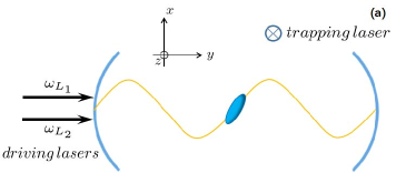
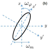
Figure 1: (a) The nanodiamond is levitated by the trapping laser and is placed in a cavity. The trapping laser propagates along the z-axis. The cavity is driven by two lasers of frequencies ${\omega_{{L_{1}}}}$ and ${\omega_{{L_{2}}}}$ (b) Details of the nanoparticle: $\left({x,y,z}\right)$ is the coordinate system of the cavity. The x-axis aligns with the polarization direction of the trapping laser. $\left({x^{\prime},y^{\prime},z^{\prime}}\right)$ is the coordinate fixed on the nanoparticle. The x’-axis aligns with the long axis of the nanoparticle.

As shown in Fig. 1, we consider a system that contains an optical cavity and an ellipsoidal nanoparticle levitated by a trapping laser. The trapping laser is linearly polarized. Therefore, both location and direction of the nanoparticle are fixed Hoang2016 . The nanoparticle has translational mode $b$ with frequency ${\omega_{m}}$ and librational mode $c$ with frequency ${\omega_{\varphi}}$. They are both coupled to the cavity mode $a$. The frequency of the mode $c$ is usually much larger than the frequency of the mode $b$. The optical mode is driven by two lasers of frequencies ${\omega_{{L_{1}}}}$ and ${\omega_{{L_{2}}}}$. The Hamiltonian of the system can be divided into three parts: ${H_{E}}$, ${H_{I}}$ and ${H_{D}}$. Such that

$$H={H_{E}}+{H_{I}}+{H_{D}}$$ (1)

where

$${H_{E}}=\hbar{\omega_{\rm{0}}}{a^{\dagger}}a+\hbar{\omega_{m}}{b^{\dagger}}b+\hbar{\omega_{\varphi}}{c^{\dagger}}c$$ (2)

$${H_{I}}=\hbar{g_{ab}}{a^{\dagger}}a\left({{b^{\dagger}}+b}\right)+\hbar{g_{ac}}{a^{\dagger}}a\left({{c^{\dagger}}+c}\right)$$ (3)

$${H_{D}}=\frac{{h{\Omega_{\rm{1}}}}}{2}\left({{a^{\dagger}}{e^{-i{\omega_{{L_{\rm{1}}}}}t}}+a{e^{i{\omega_{{L_{\rm{1}}}}}t}}}\right){\rm{+}}\frac{{h{\Omega_{\rm{2}}}}}{2}\left({{a^{\dagger}}{e^{-i{\omega_{{L_{2}}}}t}}+a{e^{i{\omega_{{L_{2}}}}t}}}\right)$$ (4)

Here $H_{E}$ is the energy term of translational mode $b$, librational mode $c$ and cavity mode $a$. $H_{I}$ describes the couplings between cavity mode $a$ and two mechanical modes $b$ and $c$. The coupling rates ${g_{ab}}$ and ${g_{ac}}$ are small, but they can be amplified by the driving lasers $H_{D}$. We will discuss how to derive the effective Hamiltonian between $a$ and $b$, $c$ modes in the next section.

III The effective Hamiltonian

We firstly consider an ideal system without decay. In order to get the effective Hamiltonian between the cavity mode $a$ and mechanical modes $b$ and $c$, we first give the Heisenberg equation corresponding to (1).

$$\begin{split}\dot{a}=&-i{\omega_{0}}a-i{g_{ab}}a\left({{b^{\dagger}}+b}\right)-i{g_{ac}}a\left({{c^{\dagger}}+c}\right)\\ &-i\frac{{{\Omega_{1}}}}{2}{e^{-i{\omega_{{L_{1}}}}t}}-i\frac{{{\Omega_{2}}}}{2}{e^{-i{\omega_{{L_{2}}}}t}}.\end{split}$$ (5)

To deal with it, we make a semi-classical ansatz

$$a={a_{0}}\left(t\right)+{\alpha_{1}}\left(t\right){e^{-i{\omega_{{L_{\rm{1}}}}}t}}+{\alpha_{2}}\left(t\right){e^{-i{\omega_{{L_{2}}}}t}}$$ (6)

where ${\alpha_{1}}$ and ${\alpha_{2}}$ are the classical amplitudes of mode $a$ with frequencies $\omega_{L1}$ and $\omega_{L2}$, and $a_{0}$ is the quantum fluctuation operator.

Inserting (6) into (5), we get the equation for the classical amplitudes $\alpha_{1}$ and $\alpha_{2}$

$$\begin{array}[]{l}-i{\omega_{{L_{\rm{1}}}}}\alpha_{1}{e^{-i{\omega_{{L_{\rm{1}}}}}t}}-i{\omega_{{L_{2}}}}\alpha_{2}{e^{-i{\omega_{{L_{2}}}}t}}+\dot{\alpha}_{1}{e^{-i{\omega_{{L_{\rm{1}}}}}t}}+\dot{\alpha}_{2}{e^{-i{\omega_{{L_{2}}}}t}}=\\ -i{\omega_{0}}\alpha_{1}{e^{-i{\omega_{{L_{\rm{1}}}}}t}}-i{\omega_{0}}\alpha_{2}{e^{-i{\omega_{{L_{2}}}}t}}-i\frac{{{\Omega_{1}}}}{2}{e^{-i{\omega_{{L_{1}}}}t}}-i\frac{{{\Omega_{2}}}}{2}{e^{-i{\omega_{{L_{2}}}}t}}.\end{array}$$ (7)

As $\alpha_{1}$ and $\alpha_{2}$ have different frequencies, we have equations for each of them

$$\dot{\alpha}_{1}= -i{\omega_{0}}\alpha_{1}+i{\omega_{{L_{\rm{1}}}}}\alpha_{1}-i\frac{{{\Omega_{1}}}}{2}$$ (8)

$$\dot{\alpha}_{2}= -i{\omega_{0}}\alpha_{2}+i{\omega_{{L_{2}}}}\alpha_{2}-i\frac{{{\Omega_{2}}}}{2}$$

So we can get their classical steady state amplitude ($\dot{\alpha}_{1}=\dot{\alpha}_{2}=0$): $\alpha_{1}=\frac{{{\Omega_{1}}}}{{2{\Delta_{1}}}}$ and $\alpha_{2}=\frac{{{\Omega_{2}}}}{{2{\Delta_{2}}}}$, where ${\Delta_{1}}={\omega_{{L_{1}}}}-{\omega_{0}}$, ${\Delta_{2}}={\omega_{{L_{2}}}}-{\omega_{0}}$. So we get

$$a={a_{0}}{e^{-i{\omega_{0}}t}}+\frac{{{\Omega_{1}}}}{{2{\Delta_{1}}}}{e^{-i{\omega_{{L_{1}}}}t}}+\frac{{{\Omega_{2}}}}{{2{\Delta_{2}}}}{e^{-i{\omega_{{L_{2}}}}t}}$$ (9)

We can derive steady-state displacements $\beta$ and $\gamma$ for $b$ and $c$ in the same way.

$$b={b_{0}}+\beta$$ (10)

$$c={c_{0}}+\gamma$$

Where $\beta=-{g_{ab}}{{\left({\alpha_{1}^{2}+\alpha_{2}^{2}}\right)}\mathord{\left/{\vphantom{{\left({\alpha_{1}^{2}+\alpha_{2}^{2}}\right)}{{\omega_{m}}}}}\right.\kern-1.2pt}{{\omega_{m}}}}$, $\gamma=-{g_{ac}}{{\left({\alpha_{1}^{2}+\alpha_{2}^{2}}\right)}\mathord{\left/{\vphantom{{\left({\alpha_{1}^{2}+\alpha_{2}^{2}}\right)}{{\omega_{\varphi}}}}}\right.\kern-1.2pt}{{\omega_{\varphi}}}}$. We substitute (6) and (10) into Hamiltonian and in the rotating frame with $U={e^{-iH_{0}t/\hbar}}$, where ${H_{0}}=\hbar{\omega_{0}}a_{0}^{\dagger}{a_{0}}+\hbar{\omega_{m}}b_{0}^{\dagger}{b_{0}}+\hbar{\omega_{\varphi}}c_{0}^{\dagger}{c_{0}}$. The Hamiltonian ${H_{RW}}={U^{\dagger}}(H-H_{0})U$. By tuning the lasers detunings, we can get different Hamiltonian between mechanical modes and the cavity mode. The different tasks such as quantum state transfer and entanglement generating can be realized. For example, if the driving lasers fulfill ${\Delta_{1}}=-{\omega_{m}}$ , ${\Delta_{2}}=-{\omega_{\varphi}}$, we can neglect fast oscillation terms. The effective Hamiltonian reads

$${H_{RW}}=\hbar{g_{ab}}\alpha_{1}\left({a_{0}^{\dagger}b_{0}+{a_{0}}{b_{0}^{\dagger}}}\right)+\hbar{g_{ac}}\alpha_{2}\left({a_{0}^{\dagger}c_{0}+{a_{0}}{c_{0}^{\dagger}}}\right).$$ (11)

The perfect quantum state transfer between the translational and the librational modes requires $|g_{ab}\alpha_{1}|=|g_{ac}\alpha_{2}|=G$. If we initialize the system as $\left|{{\psi_{a}}\left({t=0}\right)}\right\rangle\left|{{\psi_{b}}\left({t=0}\right)}\right\rangle\left|{{\psi_{c}}\left({t=0}\right)}\right\rangle=\left|0\right\rangle\left|0\right\rangle\left|1\right\rangle$, we can get

$$\begin{split}\left|{{\psi_{a}}{\psi_{b}}{\psi_{c}}\left(t\right)}\right\rangle=&\frac{1}{2}\left({1+\cos\sqrt{2}Gt}\right)\left|{001}\right\rangle\\ &-\frac{1}{2}\left({1-\cos\sqrt{2}Gt}\right)\left|{010}\right\rangle\\ &-\frac{{i\sqrt{2}}}{2}\sin\sqrt{2}Gt\left|{100}\right\rangle.\end{split}$$ (12)

If we let $t=\frac{\pi}{{\sqrt{2}G}}$, we can transfer a state from librational mode to translation mode (vice versa).

If we set ${\Delta_{1}}{\rm{+}}{\omega_{m}}{\rm{=}}{\Delta_{\rm{2}}}{\rm{+}}{\omega_{\varphi}}=\delta$, and in the large detuning limit $\delta\gg|g_{ab}\alpha_{1}|,|g_{ac}\alpha_{2}|$, the cavity mode can be adiabatically eliminated James2007 . Here we including all fast rotating terms, both rotating wave and anti-rotating wave. If the cavity mode $a_{0}$ is initially in the vacuum state, the effective Hamiltonian is

$${H_{eff}}=\hbar{G_{1}}b_{0}^{\dagger}{b_{0}}+\hbar{G_{2}}c_{0}^{\dagger}{c_{0}}+\hbar{G_{3}}\left({b_{0}^{\dagger}{c_{0}}+{b_{0}}c_{0}^{\dagger}}\right)$$ (13)

where

$${G_{1}}=\frac{{\alpha_{1}^{2}g_{ab}^{2}}}{{{\Delta_{1}}+{\omega_{m}}}}+\frac{{\alpha_{1}^{2}g_{ab}^{2}}}{{{\Delta_{1}}-{\omega_{m}}}}+\frac{{\alpha_{2}^{2}g_{ab}^{2}}}{{{\Delta_{2}}+{\omega_{m}}}}+\frac{{\alpha_{2}^{2}g_{ab}^{2}}}{{{\Delta_{2}}-{\omega_{m}}}}$$ (14)

$$G_{2}=\frac{{\alpha_{2}^{2}g_{ac}^{2}}}{{{\Delta_{2}}+{\omega_{\varphi}}}}+\frac{{\alpha_{2}^{2}g_{ac}^{2}}}{{{\Delta_{2}}-{\omega_{\varphi}}}}+\frac{{\alpha_{1}^{2}g_{ac}^{2}}}{{{\Delta_{1}}+{\omega_{\varphi}}}}+\frac{{\alpha_{1}^{2}g_{ac}^{2}}}{{{\Delta_{1}}-{\omega_{\varphi}}}}$$ (15)

.

$$G_{3}=\left({\frac{{{\alpha_{\rm{1}}}{\alpha_{2}}{g_{ab}}{g_{ac}}}}{{{\Delta_{1}}+{\omega_{m}}}}+\frac{{{\alpha_{\rm{1}}}{\alpha_{2}}{g_{ab}}{g_{ac}}}}{{{\Delta_{1}}-{\omega_{\varphi}}}}}\right)$$ (16)

If $G_{1}=G_{2}$ (we will provide workable parameters in next section), and we take the initial state as $\left|{{\psi_{b}}\left({t=0}\right)}\right\rangle\left|{{\psi_{c}}\left({t=0}\right)}\right\rangle=\left|0\right\rangle\left|1\right\rangle$, we can get

$$\begin{split}\left|{{\psi_{b}}\left(t\right)}\right\rangle\left|{{\psi_{c}}\left(t\right)}\right\rangle&=\frac{1}{2}\left({{e^{-i\left({{G_{1}}+{G_{3}}}\right)t}}+{e^{-i\left({{G_{1}}-{G_{3}}}\right)t}}}\right)\left|0\right\rangle\left|1\right\rangle\\ &+\frac{1}{2}\left({{e^{-i\left({{G_{1}}+{G_{3}}}\right)t}}-{e^{-i\left({{G_{1}}-{G_{3}}}\right)t}}}\right)\left|1\right\rangle\left|0\right\rangle.\end{split}$$ (17)

In the lab reference frame, we have

$$\begin{split}\left|{{\psi_{b}}\left(t\right)}\right\rangle\left|{{\psi_{c}}\left(t\right)}\right\rangle=&\frac{1}{2}{e^{-i{\omega_{\varphi}}t}}\left({{e^{-i\left({{G_{1}}+{G_{3}}}\right)t}}+{e^{-i\left({{G_{1}}-{G_{3}}}\right)t}}}\right)\left|0\right\rangle\left|1\right\rangle\\ +&\frac{1}{2}{e^{-i{\omega_{m}}t}}\left({{e^{-i\left({{G_{1}}+{G_{3}}}\right)t}}-{e^{-i\left({{G_{1}}-{G_{3}}}\right)t}}}\right)\left|1\right\rangle\left|0\right\rangle.\end{split}$$ (18)

If we let $t=\frac{\pi}{{2G_{3}^{2}}}$ , we can transfer a state from librational mode to translational mode (vice versa).

We can also choose ${\Delta_{1}}{\rm{-}}{\omega_{m}}{\rm{=}}{\Delta_{\rm{2}}}{\rm{-}}{\omega_{\varphi}}=\delta$. In the limit $\delta\gg G$, we can adiabatically eliminate the cavity mode, and get a two-mode-squeezing effective Hamiltonian Yin2009 ; Li2013

$${H_{RW}}=\hbar{G^{\prime}_{1}}\left({b_{0}^{\dagger}{b_{0}}+c_{0}^{\dagger}{c_{0}}}\right)+\hbar{G^{\prime}_{3}}\left({b_{0}^{\dagger}c_{0}^{\dagger}+{b_{0}}{c_{0}}}\right).$$ (19)

which could be used for generating entanglement between modes $b_{0}$ and $c_{0}$.

IV Experimental feasibility and dissipation effects

In this section, we will provide the feasible parameters in experiment and consider the effect of dissipations. In our scheme, the steady-state amplitudes $\alpha_{1}$ and $\alpha_{2}$ are in the order of ${10^{4}}$ to ${10^{5}}$. Therefore, the strength of linear couplings between cavity mode and the mechanical modes are enhanced by ${10^{4}}$ to ${10^{5}}$ times. The photon number fluctuation is in the order of $\sqrt{\alpha_{1,2}}\sim{10^{2}}$, which is relating with non-linear coupling between the cavity and the mechanical modes. Therefore, the linear coupling strength is ${10^{2}}$ times larger than the non-linear coupling strength. The effect of the photon number fluctuation is negligible in our scheme.

In experiments, the dissipation by cavity mode and mechanical modes decay is inevitable. However, in high vacuum, the mechanical decay rates are much less than the cavity decay rate Hoang2016 ; Stickler2016a ; Zhong2016 . Therefore, we only need to consider the cavity decay effect. Considering the dissipation, the steady-amplitudes will change and we can derive them by adding a term of $-i\hbar\frac{\kappa}{2}{a^{\dagger}}a$ into Hamiltonian (1). Following the same procedure mentioned above, we can get

$$\begin{split}{\alpha_{1}}=\frac{{{\Omega_{1}}}}{{2\left({{\Delta_{1}}+i\frac{\kappa}{2}}\right)}}\\ {\alpha_{2}}=\frac{{{\Omega_{2}}}}{{2\left({{\Delta_{2}}+i\frac{\kappa}{2}}\right)}}\end{split}$$ (20)

And in order to maintain the form of the Hamiltonian, we should do the transformation ${b_{0}}\to{{{\alpha_{1}}{b_{0}}}\mathord{\left/{\vphantom{{{\alpha_{1}}{b_{0}}}{\left|{{\alpha_{1}}}\right|}}}\right.\kern-1.2pt}{\left|{{\alpha_{1}}}\right|}},b_{0}^{\dagger}\to{{\alpha_{1}^{*}b_{0}^{\dagger}}\mathord{\left/{\vphantom{{\alpha_{1}^{*}b_{0}^{\dagger}}{\left|{{\alpha_{1}}}\right|}}}\right.\kern-1.2pt}{\left|{{\alpha_{1}}}\right|}}$ and ${c_{0}}\to{{{\alpha_{2}}{c_{0}}}\mathord{\left/{\vphantom{{{\alpha_{2}}{c_{0}}}{\left|{{\alpha_{2}}}\right|}}}\right.\kern-1.2pt}{\left|{{\alpha_{2}}}\right|}},c_{0}^{\dagger}\to{{\alpha_{2}^{*}c_{0}^{\dagger}}\mathord{\left/{\vphantom{{\alpha_{2}^{*}c_{0}^{\dagger}}{\left|{{\alpha_{2}}}\right|}}}\right.\kern-1.2pt}{\left|{{\alpha_{2}}}\right|}}$. Using perturbation theory Chang2010 ; Buck2003 , we can obtain the coupling constants in the same way with Ref. Hoang2016 . If we restrict the librational motion of the long axis of the nanoparticle in the plane $xOy$, we get

$$\begin{split}{g_{ab}}=&\sqrt{\frac{\hbar}{{2M{\omega_{m}}}}}\frac{{32{\pi^{2}}c{e^{-\frac{{4\pi\left({{x^{2}}+{z^{2}}}\right)}}{{\lambda L}}}}\cos ky\sin ky}}{{{\varepsilon_{0}}{\lambda^{3}}{L^{2}}}}\\ &\cdot\left({{s_{2}}+{{\cos}^{2}}\varphi\left({{s_{1}}-{s_{2}}}\right)}\right),\end{split}$$ (21)

$${g_{ac}}=\sqrt{\frac{\hbar}{{2I{\omega_{\varphi}}}}}\frac{{8\pi c{e^{-\frac{{4\pi\left({{x^{2}}+{z^{2}}}\right)}}{{\lambda L}}}}{{\cos}^{2}}ky}}{{{\varepsilon_{0}}{\lambda^{2}}{L^{2}}}}\left({{s_{1}}-{s_{2}}}\right)\sin 2\varphi.$$ (22)

Here $L$ is the length of the cavity, $\lambda$ and $k$ is the wavelength and wavenumber of cavity mode. $M$ and $I$ is the mass and the moment of inertia of the nanoparticle. ${s_{1}}$ and ${s_{2}}$ are the diagonal elements of susceptibility matrix. $\left({x,y,z,\varphi}\right)$ are the parameters describe the position of the nanoparticle: $\left({x,y,z}\right)$ are the coordinates of the center of mass (origin is the center of the cavity), $\varphi$ is the angle between the long axis of the nanoparticle and $x$-axis. $x$, $y$, $z$ and $\varphi$ can be changed by adjusting the trapping laser. For example, we choose the angle between the polarization direction of the trapping laser and the y-axis ($\varphi$) as ${45^{\circ}}$, the equilibrium position of the center of mass is$\left({0,\pi/4k,0}\right)$. We can get ${g_{ab}}/2\pi=0.3056$ Hz and ${g_{ac}}/2\pi=0.2189$ Hz. (The parameter of the nano particle we choose: $\rho=3500~{}{{{\rm{kg}}}\mathord{\left/{\vphantom{{{\rm{kg}}}{{{\rm{m}}^{\rm{3}}}}}}\right.\kern-1.2pt}{{{\rm{m}}^{\rm{3}}}}}$, long axis $a=50$ nm, short axis $b=25$ nm, ${\varepsilon_{r}}=5.7$, waist of the trapping laser ${W_{t}}=600$ nm, power of the trapping laser is $100$ mW, wavelength ${\lambda_{cav}}=1540$ nm, length of the cavity $L=10$ mm) And in this situation, ${{{\omega_{m}}}\mathord{\left/{\vphantom{{{\omega_{m}}}{2\pi}}}\right.\kern-1.2pt}{2\pi}}=247.7$ kHz, ${{{\omega_{\varphi}}}\mathord{\left/{\vphantom{{{\omega_{\varphi}}}{2\pi}}}\right.\kern-1.2pt}{2\pi}}=2.6$ MHz. If the finesse of our cavity $\mathcal{F}=10^{5}$ and we can get ${\kappa\mathord{\left/{\vphantom{\kappa{2\pi}}}\right.\kern-1.2pt}{2\pi}}=75.2$ kHz. For example we let ${\delta\mathord{\left/{\vphantom{\delta{2\pi}}}\right.\kern-1.2pt}{2\pi}}=200$ kHz, ${{{\Omega_{1}}}\mathord{\left/{\vphantom{{{\Omega_{1}}}{{\rm{2}}\pi}}}\right.\kern-1.2pt}{{\rm{2}}\pi}}={\rm{2}}{\rm{.66}}\times{10^{{\rm{9}}}}$ Hz, ${{{\Omega_{2}}}\mathord{\left/{\vphantom{{{\Omega_{2}}}{{\rm{2}}\pi}}}\right.\kern-1.2pt}{{\rm{2}}\pi}}=5.0\times{10^{10}}$ Hz. And we can get ${G_{3}\mathord{\left/{\vphantom{G{2\pi}}}\right.\kern-1.2pt}{2\pi}}=25$ kHz and time of state transfer $t=1\times{10^{-5}}$ s thus it’s not difficult to realize.

IV.1 Large detuning scheme

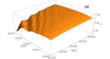
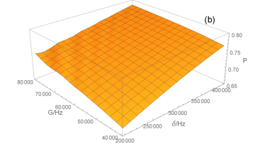
Figure 2: (a) Fidelity of state transfer as a function of $G$ and $\delta$ in the situation of large detuning. (b) The probability of the system being in this state as a function of $G$ and $\delta$.

Under the large detuning condition that ${\Delta_{1}}{\rm{+}}{\omega_{m}}{\rm{=}}{\Delta_{\rm{2}}}{\rm{+}}{\omega_{\varphi}}=\delta\gg G$, we change the system Hamiltonian to the rotating wave frame, and neglect the fast rotating terms in $H_{RW}$. In order to deal with the cavity loss effects, here we adopt the conditional Hamiltonian Plenio1998 ; Huang2016 . We assume that cavity decay rate is weak. Therfore, we can only consider the situation that system evolves without photon leakage. Under the condition that no photon is leaking out, we get the conditional Hamiltonian from quantum trajectory method Plenio1998

$$\begin{split}H=&\hbar G\left({a_{0}^{\dagger}b_{0}{e^{-i\delta t}}+{a_{0}}{b_{0}^{\dagger}}{e^{i\delta t}}}\right)+\hbar G\left({a_{0}^{\dagger}c_{0}{e^{-i\delta t}}+{a_{0}}{c_{0}^{\dagger}}{e^{i\delta t}}}\right)\\ &-i\hbar\frac{\kappa}{2}a_{0}^{\dagger}{a_{0}},\end{split}$$ (23)

where $\kappa$ is the decay rate of the cavity mode $a$. We can use the above conditional Hamiltonian to calsulate the possibility $P$ of the system evolving without photon leakage. Because we suppose that the initial state of the system is${\left|0\right\rangle_{a}}{\left|{01}\right\rangle_{bc}}$, so the subspace only includes 3 basis states:${\left|0\right\rangle_{a}}{\left|{01}\right\rangle_{bc}}$, ${\left|0\right\rangle_{a}}{\left|{10}\right\rangle_{bc}}$ and ${\left|1\right\rangle_{a}}{\left|{00}\right\rangle_{bc}}$. And at any time $t$, the state of the system is

$$\begin{split}\left|{\psi_{d}\left(t\right)}\right\rangle=&{C_{d1}}\left(t\right){\left|0\right\rangle_{a}}{\left|{01}\right\rangle_{bc}}+{C_{d2}}\left(t\right){\left|0\right\rangle_{a}}{\left|{10}\right\rangle_{bc}}\\ &+{C_{d3}}\left(t\right){\left|1\right\rangle_{a}}{\left|{00}\right\rangle_{bc}}\end{split}$$ (24)

where

$${C_{d1}}\left(t\right)=\frac{1}{2}+\frac{{\left({2\delta+i\kappa+\chi}\right)}}{{4\chi}}{e^{-i{E_{3}}t/\hbar}}-\frac{{\left({2\delta+i\kappa-\chi}\right)}}{{4\chi}}{e^{-i{E_{2}}t/\hbar}},$$ (25)

$${C_{d2}}\left(t\right)=-\frac{1}{2}+\frac{{\left({2\delta+i\kappa+\chi}\right)}}{{4\chi}}{e^{-i{E_{3}}t/\hbar}}-\frac{{\left({2\delta+i\kappa-\chi}\right)}}{{4\chi}}{e^{-i{E_{2}}t/\hbar}},$$ (26)

$$\begin{split}{C_{d3}}\left(t\right)=&-\frac{{{e^{-i\delta t}}\left({2\delta+i\kappa+\chi}\right)\left({2\delta+i\kappa-\chi}\right)}}{{16G\chi}}\cdot\\ &\left({{e^{-i{E_{3}}t/\hbar}}-{e^{-i{E_{2}}t/\hbar}}}\right)\end{split}$$ (27)

here $\chi=\sqrt{4{\delta^{2}}+32{G^{2}}+4i\delta\kappa-{\kappa^{2}}}$, ${E_{2}}=\frac{1}{4}\left({-2\delta-i\kappa-\chi}\right)$, ${E_{3}}=\frac{1}{4}\left({-2\delta-i\kappa+\chi}\right)$.

We first normalize the state $\left|\psi_{d}\right\rangle$ to calculate the fidelity, we can get $\left|{{\psi_{dn}}}\right\rangle={{\left|{{\psi_{d}}}\right\rangle}\mathord{\left/{\vphantom{{\left|{{\psi_{d}}}\right\rangle}{\sqrt{{{\left|{{C_{d1}}}\right|}^{2}}+{{\left|{{C_{d2}}}\right|}^{2}}+{{\left|{{C_{d3}}}\right|}^{2}}}}}}\right.\kern-1.2pt}{\sqrt{{{\left|{{C_{d1}}}\right|}^{2}}+{{\left|{{C_{d2}}}\right|}^{2}}+{{\left|{{C_{d3}}}\right|}^{2}}}}}$. As shown in Fig. 2(a), we plot the fidelity $F=\left|{\left\langle{{\psi_{dn}}\left(t\right)\left|{010}\right.}\right\rangle}\right|$ at the time $t=\frac{{\pi\delta}}{{2{G^{2}}-{{{\kappa^{2}}}\mathord{\left/{\vphantom{{{\kappa^{2}}}{16}}}\right.\kern-1.2pt}{16}}}}$ which can be directly derived from the strict solution of the Schrödinger Equation and ${\kappa\mathord{\left/{\vphantom{\kappa{2\pi}}}\right.\kern-1.2pt}{2\pi}}=75.2$kHz as a function of $\delta$ and $G$. The possibility of the system evolving without photon leakage is $P={\left|{{C_{d1}}}\right|^{2}}+{\left|{{C_{d2}}}\right|^{2}}+{\left|{{C_{d3}}}\right|^{2}}$. It is found that the fidelity could approach to $1$ when $G$ is small and $\delta$ is large. However, at this regime, the effective coupling between two mechanical modes is also pretty small. In Fig. 2(b), we plot $P$ as a function of $\delta$ and $G$ as well. When we choose $\delta=200$kHz and $G=50$kHz, the fidelity $F=0.95$ and the successful possibility $P=0.68$.

IV.2 Resonant scheme

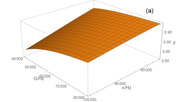
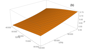
Figure 3: (a) Fidelity of state transfer as a function of $G$ and $\kappa$ in the situation of resonance. (b) The probability of the system being in this state as a function of $G$ and $\kappa$.

In resonance case, the Hamiltonian reads in

$$H=\hbar G\left({a_{0}^{\dagger}b_{0}+{a_{0}}{b_{0}^{\dagger}}}\right)+\hbar G\left({a_{0}^{\dagger}c_{0}+{a_{0}}{c_{0}^{\dagger}}}\right)-i\hbar\frac{\kappa}{2}a_{0}^{\dagger}{a_{0}}$$ (28)

Because we suppose that the initial state of the system is${\left|0\right\rangle_{a}}{\left|{01}\right\rangle_{bc}}$, the subspace only includes 3 basis states:${\left|0\right\rangle_{a}}{\left|{01}\right\rangle_{bc}}$, ${\left|0\right\rangle_{a}}{\left|{10}\right\rangle_{bc}}$ and ${\left|1\right\rangle_{a}}{\left|{00}\right\rangle_{bc}}$ as well. And at any time $t$, the state of the system is

$$\begin{split}\left|{{\psi_{r}}\left(t\right)}\right\rangle=&{C_{r1}}\left(t\right){\left|0\right\rangle_{a}}{\left|{01}\right\rangle_{bc}}+{C_{r2}}\left(t\right){\left|0\right\rangle_{a}}{\left|{10}\right\rangle_{bc}}\\ &+{C_{r3}}\left(t\right){\left|1\right\rangle_{a}}{\left|{00}\right\rangle_{bc}}\end{split}$$ (29)

and

$$\begin{split}{C_{r1}}\left(t\right)=&\frac{1}{2}+\frac{1}{2}{e^{-{{\kappa t}\mathord{\left/{\vphantom{{\kappa t}4}}\right.\kern-1.2pt}4}}}\cos\frac{{\sqrt{32{G^{2}}-{\kappa^{2}}}}}{4}t\\ &+\frac{\kappa}{{\sqrt{32{G^{2}}-{\kappa^{2}}}}}{e^{-{{\kappa t}\mathord{\left/{\vphantom{{\kappa t}4}}\right.\kern-1.2pt}4}}}\sin\frac{{\sqrt{32{G^{2}}-{\kappa^{2}}}}}{4}t,\end{split}$$ (30)

$$\begin{split}{C_{r2}}\left(t\right)=&-\frac{1}{2}+\frac{1}{2}{e^{-{{\kappa t}\mathord{\left/{\vphantom{{\kappa t}4}}\right.\kern-1.2pt}4}}}\cos\frac{{\sqrt{32{G^{2}}-{\kappa^{2}}}}}{4}t\\ &+\frac{\kappa}{{\sqrt{32{G^{2}}-{\kappa^{2}}}}}{e^{-{{\kappa t}\mathord{\left/{\vphantom{{\kappa t}4}}\right.\kern-1.2pt}4}}}\sin\frac{{\sqrt{32{G^{2}}-{\kappa^{2}}}}}{4}t,\end{split}$$ (31)

$${C_{r3}}\left(t\right)=-i\frac{{4G}}{{\sqrt{32{G^{2}}-{\kappa^{2}}}}}{e^{-{{\kappa t}\mathord{\left/{\vphantom{{\kappa t}4}}\right.\kern-1.2pt}4}}}\sin\frac{{\sqrt{32{G^{2}}-{\kappa^{2}}}}}{4}t.$$ (32)

Same as the large detuning case, we plot the fidelity $F=\left|{\left\langle{{\psi_{nr}}\left(t\right)\left|{010}\right.}\right\rangle}\right|$ in Fig. 3(a) and possibility $P={\left|{{C_{r1}}}\right|^{2}}+{\left|{{C_{r2}}}\right|^{2}}+{\left|{{C_{r3}}}\right|^{2}}$ at $t=\frac{{4\pi}}{{\sqrt{32{G^{2}}-{\kappa^{2}}}}}$ in Fig. 3(b) as a function of $G$ and $\kappa$. Here $\left|{{\psi_{nr}}\left(t\right)}\right\rangle$ is the normalized state of $\left|{\psi_{r}\left(t\right)}\right\rangle$. It is found that both $P$ and $F$ are in favor of larger $G$ and less $\kappa$. When we choose $\kappa=75.2$kHz and $G=50$kHz, the fidelity $F=0.926$ and the successful possibility $P=0.59$. As we can see, for both large detuning and resonant schemes, the quantum state transfer could be realized with pretty high fidelty and successful possibility. In experiment, we can choose either of them for convenience.

V conclusion

In this paper, we propose a scheme to couple librational and translational modes of a levitated nanoparticle with an optical cavity mode. We discuss how to realize quantum state transfer from a librational mode to a translational mode, and vice versa. We also discuss effects of cavity decay on the fidelity of state transfer. We find that the high-fidelity state transfer could be realized under practical experimental conditions.

Funding and Acknowledgement

National Natural Science Foundation of China (61435007); Joint Foundation of Ministry of Education of China; National Science Foundation (NSF) (1555035-PHY).
We would like to thank Yue Ma for the helpful discussions.

References

- (1) M. Aspelmeyer, T. J. Kippenberg, and F. Marquardt, “Cavity optomechanics,” Rev. Mod. Phys. 86, 1391 (2014).
- (2) M. Poot and H. S. J. van der Zant, “Mechanical systems in the quantum regime,” Phys. Rep. 511, 273 (2012).
- (3) A. D. O’Connell, M. Hofheinz, M. Ansmann, R. C. Bialczak, M. Lenander, E. Lucero, M. Neeley, D. Sank, H. Wang, and M. Weides, J. Wenner, John M. Martinis, and A. N. Cleland, “Quantum ground state and single-phonon control of a mechanical resonator,” Nature 464, 697 (2010).
- (4) J. Chan, T. P. M. Alegre, A. H. Safavi-Naeini, J. T. Hill, A. Krause, S. Gröblacher, M. Aspelmeyer, O, Painter, “Laser cooling of a nanomechanical oscillator into its quantum ground state,” Nature, 478, 89 (2011).
- (5) Y. Chen, “Macroscopic quantum mechanics: theory and experimental concepts of optomechanics,” J. Phys. B: At. Mol. Opt. Phys. 46, 104001 (2013).
- (6) Z.-q. Yin, T. Li. “Bringing quantum mechanics to life: from Schrödinger’s cat to Schrödinger’s microbe,” Contemp. Phys. 58, 119 (2017).
- (7) J. D. Teufel, T. Donner, M. A. Castellanos-Beltran, J. W. Harlow, K. W. Lehnert, “Nanomechanical motion measured with an imprecision below that at the standard quantum limit,” Nat. Nanotech. 4, 820 (2009).
- (8) Z. Q. Yin, W. L. Yang, L. Sun, and L. M. Duan, “Quantum network of superconducting qubits through an optomechanical interface,” Phys. Rev. A 91, 012333 (2015).
- (9) H.-K. Li, X.-X. Ren, Y.-C. Liu, and Y.-F. Xiao, “Photon-photon interactions in a largely detuned optomechanical cavity,” Phys. Rev. A 88, 053850 (2013).
- (10) T. Li, S. Kheifets, and M. G. Raizen. “Millikelvin cooling of an optically trapped microsphere in vacuum,” Nature Phys. 7, 527 (2011).
- (11) O. Romero-Isart, M. L. Juan, R. Quidant, and J. I. Cirac, “Toward quantum superposition of living organisms,” New J. Phys. 12, 033015 (2010).
- (12) V. Jain, J. Gieseler, C. Moritz, C. Dellago, R. Quidant, and L. Novotny, “Direct Measurement of Photon Recoil from a Levitated Nanoparticle,” Phys. Rev. Lett. 116, 243601 (2016).
- (13) D. E. Chang, C. A. Regal, S. B. Papp, D. J. Wilson, J. Ye, O. Painter, H. J. Kimble, and P. Zoller, “Cavity opto-mechanics using an optically levitated nanosphere,” Proc Natl Acad Sci U S A 107, 1005 (2010).
- (14) G Ranjit, M Cunningham, K Casey, A. A. Geraci, “Zeptonewton force sensing with nanospheres in an optical lattice,”, Phys. Rev. A 93, 053801 (2016).
- (15) A. D. Rider, D. C. Moore, C. P. Blakemore, M. Louis, M. Lu, and G. Gratta. “Search for screened interactions associated with dark energy below the 100 m length scale,” Phys. Rev. Lett. 117, 101101 (2016).
- (16) D.C. Moore, A.D. Rider, G. Gratta. “Search for Millicharged Particles Using Optically Levitated Microspheres,” Phys. Rev. Lett. 113, 251801 (2014).
- (17) O. Romero-Isart, A. C. Pflanzer, F. Blaser, R. Kaltenbaek, N. Kiesel, M. Aspelmeyer, and J. I. Cirac, “Large Quantum Superpositions and Interference of Massive Nanometer-Sized Objects,” Phys. Rev. Lett. 107, 020405 (2011).
- (18) Z. Yin, T. Li, X. Zhang, and L. Duan, “Large quantum superpositions of a levitated nanodiamond through spin-optomechanical coupling,” Phys. Rev. A 88, 033614 (2013).
- (19) H. Shi and M. Bhattacharya, “Optomechanics based on angular momentum exchange between light and matter,” J. Phys. B: At. Mol. Opt. Phys. 49, 153001 (2016).
- (20) H Shi, M Bhattacharya, “Coupling a small torsional oscillator to large optical angular momentum,” J. Mod. Opt. 60, 382 (2013).
- (21) T. M. Hoang, Y. Ma, J. Ahn, J. Bang, F. Robicheaux, Z. Yin, and T. Li, “Torsional Optomechanics of a Levitated Nonspherical Nanoparticle,” Phys. Rev. Lett. 117, 123604 (2016).
- (22) B. A. Stickler, S. Nimmrichter, L. Martinetz, S. Kuhn, M. Arndt, and K. Hornberger, “Ro-translational cavity cooling of dielectric rods and disks,” Phys. Rev. A 94, 033818 (2016).
- (23) Stefan Kuhn, Alon Kosloff, Benjamin A. Stickler, Fernando Patolsky, Klaus Hornberger, Markus Arndt, and James Millen, ”Full rotational control of levitated silicon nanorods,” Optica 4, 356 (2017).
- (24) P. Nagornykh, J. E. Coppock, J. P. J. Murphy, B. E. Kane, “Optical and magnetic measurements of gyroscopically stabilized graphene nanoplatelets levitated in an ion trap,” arXiv:1612.05928 (2016).
- (25) C. Zhong, F. Robicheaux, “Shot noise dominant regime of a nanoparticle in a laser beam,” arXiv:1701.04477 (2017).
- (26) F. Marquardt, J. P. Chen, A. Clerk, and S. Girvin, “Quantum Theory of Cavity-Assisted Sideband Cooling of Mechanical Motion,” Phys. Rev. Lett. 99, 093902 (2007).
- (27) I. Wilson-Rae, N. Nooshi, W. Zwerger, and T. J. Kippenberg, “Theory of Ground State Cooling of a Mechanical Oscillator Using Dynamical Backaction,” Phys. Rev. Lett. 99, 093901 (2007).
- (28) M. Frimmer, J. Gieseler, and L. Novotny, “Cooling Mechanical Oscillators by Coherent Control” Phys. Rev. Lett. 117, 163601 (2016).
- (29) J. F. Ralph, K. Jacobs, and J. Coleman, “Coupling rotational and translational motion via a continuous measurement in an optomechanical sphere,” Phys. Rev. A 94, 032108 (2016).
- (30) D. James and J. Jerke, “Effective Hamiltonian theory and its applications in quantum information,” Can. J. Phys. 85, 625 (2007).
- (31) Z.-q. Yin and Y.-J. Han, “Generating EPR beams in a cavity optomechanical system,” Phys. Rev. A 79, 024301 (2009).
- (32) B. A. Stickler, B. Papendell, and K. Hornberger, “Spatio-orientational decoherence of nanoparticles,” Phys. Rev. A 94, 033828 (2016).
- (33) C. Zhong, and F. Robicheaux, “Decoherence of rotational degrees of freedom,” Phys. Rev. A 94, 052109 (2016).
- (34) Joseph R. Buck Jr, Cavity QED in microsphere and Fabry-Perot cavities. PhD Thesis. California Institute of Technology, (2003).
- (35) M. B. Plenio and P. L. Knight, “The quantum-jump approach to dissipative dynamics in quantum optics,” Rev. Mod. Phys. 70, 101 (1998).
- (36) Y. Huang, Z.-q. Yin, and W. L. Yang, “Realizing a topological transition in a non-Hermitian quantum walk with circuit QED,” Phys. Rev. A 94, 022302 (2016).