GraphZip: Dictionary-based Compression for Mining Graph Streams

Abstract.

A massive amount of data generated today on platforms such as social networks, telecommunication networks, and the internet in general can be represented as graph streams. Activity in a network’s underlying graph generates a sequence of edges in the form of a stream; for example, a social network may generate a graph stream based on the interactions (edges) between different users (nodes) over time. While many graph mining algorithms have already been developed for analyzing relatively small graphs, graphs that begin to approach the size of real-world networks stress the limitations of such methods due to their dynamic nature and the substantial number of nodes and connections involved.
In this paper we present GraphZip, a scalable method for mining interesting patterns in graph streams. GraphZip is inspired by the Lempel-Ziv (LZ) class of compression algorithms, and uses a novel dictionary-based compression approach in conjunction with the minimum description length principle to discover maximally-compressing patterns in a graph stream. We experimentally show that GraphZip is able to retrieve complex and insightful patterns from large real-world graphs and artificially-generated graphs with ground truth patterns. Additionally, our results demonstrate that GraphZip is both highly efficient and highly effective compared to existing state-of-the-art methods for mining graph streams.

1. Introduction

Graphs are used to represent data across a wide spectrum of areas, from computational chemistry to social network analysis. Graph mining is an active area of research, and there are numerous methods for mining smaller graphs (several thousand edges), but many of these systems are unable to scale to real-world graphs (e.g., social networks) with millions or even billions of edges. Conventional graph mining algorithms assume a complete static graph as input, however many real-world graphs are often too large to hold in main memory. Additionally, many real-world graphs of interest are dynamic and actively growing - Facebook, for example, records over 300 new users per minute and has a social graph with more than 400 billion edges (ChingFB, ). While it is possible to utilize conventional graph mining systems on dynamic graphs by processing static ‘snapshots’ of the graph at various points in time, in many cases the underlying data the graph represents changes at a rate so fast that attempting to analyze the data using such methods is futile.

In cases where the graph in question is inherently dynamic, we can instead treat the graph as a sequential stream of edges representing continuous updates to the graph’s overall structure. For example, given a graph modeling friendships (edges) between users (nodes) in a social network, we can consider all new or updated relationships during a set time interval (e.g., 1 hour) a set of edges from time $t_{i}$ to $t_{i+1}$. The graph mining system then processes the sequential edge sets at every interval, as opposed to attempting to read the entire graph at once. Processing large graphs in a streaming fashion drastically reduces the system’s memory requirements (since only small portions of the graph are seen at a time) and enables processing of large, dynamic real-world datasets. However, deploying a streaming model for real-time data analysis also imposes strict constraints: the system has a limited time window to process each set of edges, and edges can only be viewed once before they are replaced in memory by those in the next set.

Many graph mining algorithms aim to identify interesting patterns within an input graph. Various algorithms use different metrics to quantify how ‘interesting’ a pattern is: frequent subgraph mining (FSM) focuses on finding all subgraphs that appear in the graph over a certain frequency threshold, whereas problems such as counting motifs or finding maximal cliques in a graph (formalized in (przulj-motifs, ) and (bron-kerbosch-cliques, ), respectively) focus on discovering subgraphs with a specific structure.

This paper relies on a novel approach to identify interesting patterns in a graph - namely, finding a set of substructures that best compress the graph. More precisely, we compress a graph using a pattern (subgraph) $G$ by replacing all instances of $G$ in the graph with a new node $p$ representing $G$ (see figure 1). The reduction in size of the overall graph is a measure of the compression afforded by pattern $G$, and we search for patterns that compress the graph to the maximal extent. The same concept is found in certain types of data compression (e.g., LZ78 (lz78, ), ZIP) where the compression method looks for recurring patterns or sequences in the data stream, builds a dictionary representing the recurring patterns with shorter binary codes, and then stores the compressed data using only the binary codes and the dictionary. In the context of graphs, a byproduct of this process is that the pattern dictionary contains a set of subgraphs that compress well, and therefore represents an alternative approach for finding interesting (highly-compressing) patterns in a graph stream.

We propose a dictionary-based compression method for graph- based knowledge discovery: GraphZip. Our approach is designed to efficiently mine graph streams and uncover interesting patterns by finding maximally-compressing substructures. Specifically, our main contributions are as follows:

1. We propose a new graph mining paradigm based on the LZ class of compression algorithms.

2. Based on this paradigm, we introduce a new graph mining algorithm, GraphZip, for efficiently processing massive amounts of data from graph streams.

3. We demonstrate the effectiveness and scalability of our method using a variety of openly available synthetic and real-world datasets.

In our experiments, we demonstrate that our approach is able to retrieve both complex and insightful patterns from large real-world graphs by utilizing graph streams. In addition, we show that our approach is able to successfully mine a large class of varied substructures from artificially-generated graphs with ground truth patterns. When we compare GraphZip’s performance with that of several other state-of-the-art graph mining methods, we find that GraphZip consistently outperforms state-of-the-art methods on a variety of real-world datasets.

The GraphZip system, including all related code and data used for this paper, are available for download online. GraphZip is not to be confused with the method described in (graphzip2, ) for hierarchical clustering on spatial data, which goes by the same name.

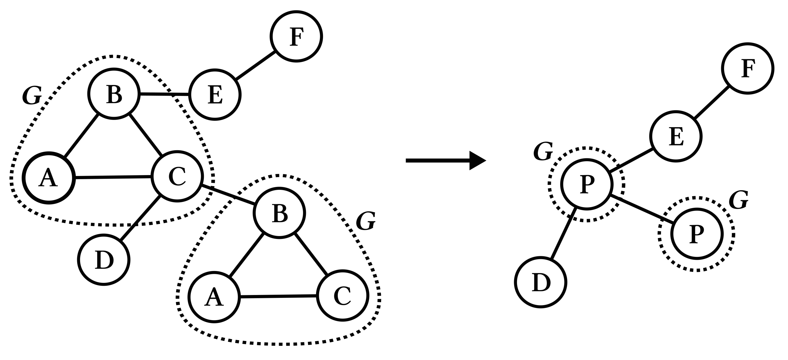
Figure 1. Compression via substitution. Vertices $A$, $B$, and $C$ form a recurring pattern (subgraph) $G$. Substituting the pattern for a single node $P$ representing $G$ reduces the graph’s overall size. The reduction in size is a measure of the compression afforded by pattern $P$.

2. Related Work

For the purposes of this paper, we classify previous work into two general categories: streaming and non-streaming.

2.1. Non-streaming

Non-streaming graph mining algorithms take as input either a single graph (single graph mining), or multiple smaller graphs (transactional mining).

Transactional mining. FSG (fsg, ) is an early approach to finding frequent subgraphs across a set of graphs, and adopts the Apriori algorithm for frequent itemset mining (apriori, ). FSG works by joining two frequent subgraphs to construct candidate subgraphs, then checking the frequency of the new candidates in the graph. gSpan (gspan, ) uses a ‘grow-and-store’ approach that extends saved subgraphs to form new ones, an improvement over FSG’s prohibitively expensive join operation. Margin (margin, ) prunes the search space to find maximal subgraphs only, a narrower and thus easier problem than FSM. CloseGraph (closegraph, ) is another method that reduces the problem space by mining only closed frequent subgraphs - subgraphs that have strictly smaller support than any existing supergraphs. Leap (leap, ) and GraphSig (graphsig, ) are two recent approaches for mining ‘significant subgraphs’ as measured by a probabilistic objective function. By mining a small set of statistically significant subgraphs as opposed to a complete set of frequent subgraphs, Leap and GraphSig are able to avoid the problem of exponential search spaces generated by FSM miners with low frequency thresholds.

Single graph mining. SUBDUE (subdue, ) is an approximate algorithm based on the branch-and-bound search technique. SUBDUE, like GraphZip, uses the Minimum Description Length (MDL) principle (mdl, ) to mine maximally-compressing patterns in the graph. However, unlike GraphZip, SUBDUE returns a restrictively small number of patterns regardless of the size of the input graph (grew, ). SUBDUE has been improved in recent years (subdue2-subgen, ; subdue3, ; subdue4, ), yet the fundamental limitations of the algorithm (in particular the branch-and-bound technique) remain the same. SEuS (seus, ) is an approximate method that creates a compressed representation of the graph by collapsing vertices that share labels. SEuS however is only effective in cases where the input graph has a small number of unique subgraphs that occur with high frequency, as opposed to when the input graph has a large number of subgraphs that appear with lower frequency. SiGram (sigram, ) is a complete method for finding frequent connected subgraphs (complete methods are guaranteed to find all solutions that fit certain constraints such as the minimum frequency threshold, unlike their approximate counterparts). SiGram adopts a grow-and-store approach similar to gSpan, but uses the expensive (NP-complete) Maximal Independent Set (MIS) metric for its frequency threshold, leading the system to be comparatively inefficient in practice. Additionally, like SEuS, SiGram suffers from a limited domain problem as it is designed specifically to mine sparse, undirected and labeled graphs only. Grew (grew, ) is another approximate method for mining frequent connected subgraphs, and is similar to SUBDUE in that Grew only discovers a relatively small subset of solutions in the search space. GraMi (grami, ) is a state-of-the-art complete method (with an approximate version AGraMi) that has been shown to be highly-efficient for FSM on a single large graph. However, the size of the input graph is still limited since GraMi requires the entire graph to be held in main memory. Arabesque (arabesque, ) is a recent distributed approach built on top of Apache Giraph (giraph, ) that can horizontally scale non-streaming algorithms (FSM, clique finding, motif counting, etc.) across multiple servers. However, horizontal scaling can be cost-prohibitive and is only capable of linearly scaling algorithms whose runtimes often grow exponentially with the size of the input graph. GERM (germ, ) and the algorithm introduced by Wackersreuther et al. (wackersreuther, ) can mine frequent subgraphs in dynamic graphs, however both methods require as input snapshots of the entire graph as opposed to incremental updates to the graph via graph streams.

2.2. Streaming

GraphScope (graphscope, ) is a parameter-free streaming method that, like GraphZip and SUBDUE, is based on the MDL principle. GraphScope encodes the graph stream with the objective of minimizing compression cost, in order to determine important change-points in the temporal data. Beyond change-point and community detection however, GraphScope has limited use for other tasks, e.g. mining interesting subgraphs. Though the model itself is parameter-free, GraphScope requires the dimensions of the graph (number of source and destination nodes) to be known a priori, and thus is unable to mine streams from dynamic graphs that introduce unseen nodes in new edge streams. Braun et al. (braun2014, ) proposed a novel data structure called DSMatrix for mining frequent patterns in dense graph streams, yet similar to GraphScope their approach requires that the edges and nodes be known beforehand, limiting its real-world applications. Aggarwal et al. (aggarwalvldb2010, ) introduced a probabilistic model for mining dense structural patterns in graph streams, however the approximation techniques used lead to the occurrence of both false positives and false negatives in the results set, reducing the method’s viability in many real-world settings. StreamFSM (streamfsm, ), based on gSpan, is a recently introduced method for frequent subgraph mining on graph streams, whose performance we compare directly with that of GraphZip (see section §4). There also exist several systems targeted at more specific graph analysis tasks in the streaming setting: counting triangles (doulion, ), outlier (aggarwalicde2011, ) and hotspot (aggarwalicdm2013, ) detection, and link prediction (zhaoicde2016, ). Summarization methods such as TCM (tcm, ), gSketch (gsketch, ) and count-min sketch (countminsketch, ) focus on constructing sketch synopses from large graph streams that can provide approximate answers to queries about the graph’s properties. For a detailed survey of state-of-the-art graph stream techniques, see (streamsurvey, ) (for a more general overview of graph mining algorithms, see (gmsurvey, )).

GraphZip can process an infinite stream of edges without requiring details about nodes or edges beforehand, and has no restrictions on the type of graph being streamed. While GraphZip is designed specifically for the streaming setting, it draws from ideas such as grow-and-store and the MDL principle originally applied in non-streaming methods. In contrast to summarization methods, GraphZip returns exact subgraphs extracted from the stream as opposed to approximate results. To the best of our knowledge, GraphZip is the first graph mining algorithm for mining maximally-compressing subgraphs from a graph stream.

Table 1. Symbol definitions. Note that $\alpha$ and $\theta$ are the hyperparameters of the GraphZip algorithm.

Symbol	Definition
$G$	Arbitrary graph
$V_{G}$	Vertex set of graph G
$E_{G}$	Edge set of graph G
$S$	Graph stream sequence
$S^{(i)}$	Graph at time $i$ of stream $S$
$B$	A batch of edges from graph stream
$P$	Pattern dictionary
$P^{(i)}$	Pattern (graph) $i$ in dictionary $P$
$V_{P^{(i)}}$	Vertex (node) set of pattern $P^{(i)}$
$E_{P^{(i)}}$	Edge set of pattern $P^{(i)}$
$C_{P^{(i)}}$	Compression score of pattern $P^{(i)}$
$F_{P^{(i)}}$	Frequency (count) of pattern $P^{(i)}$
$\alpha$	Batch size
$\theta$	Size threshold of $P$
$H(G)$	Compression scoring function
$I(G,G)$	Graph isomorphism function
$SI(G,G)$	Subgraph isomorphism function

3. Method

3.1. Preliminaries

In this section, we review the fundamental graph theory needed to formulate our approach and formalize the definitions used in the rest of the paper. See table 1 for symbol definitions.

Terminology. A graph $G$ is composed of a vertex set $V$ which contains all vertices (nodes) $v\in V$, and an edge set $E$ which contains all edges $e\in E$, each of which connects a source vertex to a target vertex. A subgraph $g$ of $G$ is a graph composed of a subset of $G$’s vertices and edges. All vertices $v\in V$ and edges $e\in E$ have a unique index which refers to its internal location in the edge or vertex list (e.g., $v_{1}$ in $V=\{v_{1},v_{2},v_{3}\}$ has index $0$, $v_{2}$ has index 1, etc.). In a vertex-labeled graph, there exists a one-to-one (i.e., unique) mapping from each vertex to a label, and in an edge-labeled graph the same mapping exists for the edge set. The value of labels within a graph is often domain-dependent: e.g., in a social network, vertex labels may correspond to a user type (e.g. ‘male’, ‘female’) while edge labels may correspond to different relationship types (e.g. ‘friend’, ‘family’, etc.).

Definition 3.1.

Isomorphism: Two graphs $G_{1}$ and $G_{2}$ are isomorphic (denoted by $G_{1}\simeq G_{2}$) if there is a one-to-one mapping between the edges and vertices of $G_{1}$ and $G_{2}$. That is, each vertex $v$ in $G_{1}$ is mapped to a unique vertex $u$ in $G_{2}$, the two of which must share the same edges, i.e., be adjacent to the same vertices (if the graph is labeled, the vertices and edges must also share the same labels). $G_{1}\simeq G_{2}$ is equivalent to $G_{1}$ and $G_{2}$ sharing the same structure.

Definition 3.2.

Subgraph isomorphism: Graph $G_{1}$ is considered a subgraph isomorphism of graph $G_{2}$ if it is an isomorphism of some subgraph $g_{2}$ of $G_{2}$. The actual instance of $g_{2}$ is called an embedding of $G_{1}$ in $G_{2}$. The subgraph isomorphism problem is a generalization of the graph isomorphism problem, and is known to be NP-complete (subiso-npcomplete, ) (unlike the graph isomorphism problem, the complexity of which is undetermined). Despite the problem’s complexity, many graph mining algorithms make heavy use of subgraph isomorphism checks for graph matching, and accordingly several optimizations have been made in the past decade which have significantly improved the efficiency of isomorphism (or subgraph isomorphism) checks in practice.

Definition 3.3.

Graph stream: A graph stream $S$ can be represented as a chronological sequence of edges drawn from a graph.

$$S=\{e_{(1)},e_{(2)},e_{(3)},...,e_{(n)}\}$$

We can process the graph stream by segmenting the stream into distinct sets of edges, each set forming a single (possibly disconnected) graph stream object. In the case of a dynamic graph, updates to the graph can be viewed as new stream objects. In the rest of the paper we also refer to graph stream objects as batches, where batch size refers to the size of the stream object’s edge set (i.e., the number of edges in the batch).

3.2. Problem Formulation

Given a graph stream and a compression scoring function $H$, our objective function equates to maximizing the cumulative compression score of the entire pattern dictionary $P$:

(1) $$f(G,H)=\operatorname*{arg\,max}_{P}\sum_{i}H(P^{(i)})$$

The direct approach to solving for $f$ would require enumerating over all possible subgraphs of $G$, a computationally intractable task in most real-world scenarios since it would require storing the entirety of the graph stream, in addition to computing subgraph isomorphism checks over the entire graph. Therefore, we employ a heuristic algorithm to approximate such a solution.

Algorithm 1 GraphZip

1:  Initialize $P$

2:  while edges remain in stream do

3:     Construct graph $B$ using $\alpha$ edges

4:     for each graph $p$ in $P$ do

5:        $E$ $\leftarrow$ subgraph isomorphisms of $p$ in $B$

6:        for each graph $g$ in $E$ do

7:           $g^{\prime}\leftarrow g.copy()$

8:           for each $e$ in $E_{g}$ do

9:              if $e$ not in $p$ then

10:                 Extend $g^{\prime}$ by new edge $e$

11:              else

12:                 Add internal edge $e$ to $g^{\prime}$

13:              end if

14:           end for

15:           Mark each extended edge $e\in B$ as used

16:           if $g^{\prime}\neq g$ then

17:              Add $g^{\prime}$ to $P$

18:           end if

19:        end for

20:     end for

21:     $R\leftarrow$ remaining unused edges in $B$

22:     Add edges in $R$ as single-edge patterns to $P$

23:  end while

24:  return  $P$

3.3. The GraphZip Algorithm

GraphZip is a highly-scalable method for discovering interesting patterns in a massive graph. Inspired by dictionary-based file compression, GraphZip builds a dictionary of highly-compressing patterns by counting previously seen patterns in the graph stream and saving new patterns that extend from old ones. The resulting dictionary contains highly-compressing patterns from the given graph stream, which can be used directly or fed into a separate non-streaming algorithm (e.g., a maximal-clique finder). While GraphZip is designed specifically with graph streams in mind, the algorithm can be easily applied to smaller static graphs without modification: if GraphZip is given as input a single graph it will automatically partition it into batches of size $\alpha$ and process the graph as a stream. If the total number of edges in the graph (or number of edges remaining after $n$ iterations) is less than $\alpha$, GraphZip will process the graph as a single batch. This flexibility between input types allows us to compare GraphZip directly with non-streaming methods.

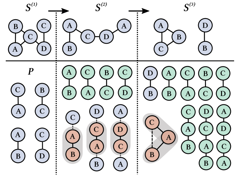
Figure 2. A simplified illustration of the GraphZip algorithm. In dictionary $P$, blue indicates a new pattern, orange indicates a matched pattern extending to a new pattern, and green indicates a non-repeated pattern. After processing $S^{(1)}$, $P$ contains only single edge patterns. $A$-$B$, $C$-$A$, and $D$-$C$ are embedded in $S^{(2)}$, so they are extended as new patterns in $P$. $C$-$A$-$B$ is embedded in $S^{(3)}$, and is extended with an internal edge as a new pattern, along with the remaining edge $D$-$B$.

The general procedure of GraphZip is illustrated in figure 2. GraphZip is initialized with an empty dictionary $P$ with max size $\theta$ (provided by the user), which maps graphs to their frequency (count) and compression score. GraphZip collects arriving edges from the graph stream into batches of size $\alpha$ (also provided by the user), and runs the $compress$ procedure on each batch $B$: if a pattern $p$ from the dictionary is embedded in $B$, GraphZip increments the frequency of the pattern in the dictionary and recomputes its compression score. Additionally, for each instance $i$ of pattern $p$ embedded in batch $B$, GraphZip extends $p$ by one edge length, tagging each of the edges from $B$ used to extend $p$. The new edges used to extend $p$ are the edges incident on $i$ that exist in batch $B$ but not in pattern $p$. GraphZip then adds the new extended pattern to $P$. After $P$ has been updated with all the extended patterns, the remaining untagged edges in $B$ are added as single-edge patterns to $P$. Our current reference implementation supports both undirected and directed edges, but not hyper-edges or self-loops. However, these limitations are implementation specific rather than inherent to the algorithm. Additionally, both representational variants can be converted to simple edges (a node and two edges).

If the dictionary exceeds size 2$\theta$, the dictionary is sorted according to the compression scores and trimmed to $\theta$. A pattern’s compression score is computed as follows:

(2) $$H(P^{(i)})=(|E_{P^{(i)}}|-1)\times(F_{P^{(i)}}-1)$$

This equates a pattern’s compressibility to a product of its size and frequency. We use $(F_{P^{(i)}}-1)$ so that a pattern with a frequency of $1$ has a compression score of $0$, since a pattern that only appears once affords no real compression to the overall graph. The same offset is applied to the pattern size in $(|E_{P^{(i)}}|-1)$ to reduce the weighting of single-edge patterns. Due to the fact that overlapping instances of a pattern in a batch are counted independently, it is possible that GraphZip will overestimate the compression value of large structures with many homomorphisms.

Note that the compression method used is intrinsically lossy, since GraphZip does not retain information on how each of the instances are connected to the rest of the graph. The main focus of our work is knowledge discovery in graph streams, so lossy compression is an appropriate trade-off for decreased complexity and increased performance. More work is necessary to make GraphZip lossless, for example in the case where it is necessary to fully reconstruct the original graph from the pattern dictionary.

See algorithm 1 for pseudo-code, and the online repository for a reference implementation.

3.4. Scalability

Speed and memory usage are critical properties of graph mining algorithms designed to mine large real-world graphs. A deployed graph mining system should be able to keep up with the flow of data in the dynamic graph setting, while summarizing a possibly infinite graph stream in memory. Memory usage in GraphZip is directly bounded by the maximum dictionary size ($\theta$), and is indirectly bounded by the batch size ($\alpha$), since the patterns within the dictionary cannot grow larger than the batch size (no subgraph isomorphisms of the pattern in the batch will exist). Both parameters $\theta$ and $\alpha$ can be modified to maximize performance given certain hardware limitations.

The bulk of the computation in the GraphZip algorithm happens while checking for embeddings of pattern $p$ in batch $B$ (find all subgraph isomorphisms of $p$ in $B$). Note that because each entry in the pattern dictionary is unique, none of the subgraph isomorphism checks are contingent on each other, and thus the loop can be naïvely parallelized across an arbitrary number of cores. This allows for large performance gains and means that an increase in dictionary size can be scaled linearly with an increase in cores. Even without parallelization of the subgraph isomorphism checks, GraphZip is still faster than other state-of-the-art graph mining systems (as described in section §4). See section §A for a formal runtime analysis.

4. Experimental Evaluation

There are two main questions we focus on when evaluating our algorithm: does it generate objectively and subjectively good results (i.e. correct and interesting results, respectively), and does it generate them in a reasonable amount of time? To answer these questions we test GraphZip on an extensive suite of synthetic and real datasets ranging from a few thousand to several million nodes and edges (see table 3). Using these datasets, we benchmark GraphZip against three state-of-the-art, openly available graph mining systems: SUBDUE, GraMi, and StreamFSM. Because there is no directly comparable method to GraphZip for mining maximally-compressing patterns in graph streams, we instead evaluate GraphZip against a non-streaming method for mining compressing patterns (SUBDUE), a non-streaming method for frequent subgraph mining (GraMi), and a streaming method for frequent subgraph mining (StreamFSM). Highly-compressing patterns are often both large and frequent, so FSM methods serve as an appropriate comparison to GraphZip.

All experiments were run on a compute server configured with an AMD Opteron 6348 processor (2.8 GHz) and 128GB of RAM.

Figure 3. We embed different types of graph substructures into our synthetic graphs, and then test to see if they are recovered. Corresponding datasets (from left to right): 3-CLIQ, 4-CLIQ, 4-STAR, 4-PATH, 8-TREE.

4.1. Synthetic graphs

To test whether our algorithm outputs correct substructures, we utilize a tool called SUBGEN (subdue2-subgen, ) to embed ground truth patterns with desired frequencies into an artificially generated graph. This allows us to test whether or not a graph mining system correctly surfaces known patterns we expect to be returned in the result set. Since both GraphZip and SUBDUE are designed to mine highly-compressing patterns from a graph, we embed large and frequent (i.e., highly-compressing) patterns in the graph, then record the number of ground truth patterns recovered. Given a set of embedded patterns $E$, and a set of patterns $R$ returned by our graph mining system, an embedded pattern $E^{(i)}\in E$ is considered matched if for some returned pattern $R^{(i)}\in R$, $R^{(i)}\simeq E^{(i)}$. Thus, we calculate the fraction $a$ of embedded patterns recovered using the scoring metric

(3) $$a=|\{E^{(i)}|E^{(i)}\in E\wedge R^{(i)}\in R\wedge E^{(i)}\simeq R^{(i)}\}|\ /\ |E|$$

Which is equivalent to

(4) $$\textit{\small accuracy}={\textit{\small matched patterns }}/{\textit{ \small total patterns}}$$

We count a ground truth pattern as matched if it is found in GraphZip’s pattern dictionary after the final batch, or in SUBDUE’s case, if it is returned directly at the end of the program.

In addition to making the ground truth patterns highly-compressing, we also design the patterns to cover a wide class of fundamental graph patterns, including cliques, paths, stars and trees (see figure 3). This allows us to discern if a method has difficulty mining a certain type of structure (e.g., a poorly designed system may have trouble detecting cycles and therefore cliques). The naming scheme for each synthetic graph dataset is N-TYPE, where $N$ is the number of vertices in the embedded pattern and TYPE is a shorthand of the pattern type (e.g., 3-CLIQ is a graph with embedded 3-cliques). All synthetic graphs in table 2 are generated with 1000 nodes, 5000 edges, and 20%, 50% or 80% coverage (the percentage of the graph covered by instances of the pattern).

Table 2. GraphZip and SUBDUE runtime and accuracy on various synthetic graphs. For runtime, lower is better. For SUBDUE, the ‘+’ for runtime indicates the program was terminated after 1000 seconds (no accuracy shown).

Dataset	Cov.	Runtime (sec.)			Accuracy (%)
	(%)	GraphZip	SUBDUE		GraphZip	SUBDUE
3-CLIQ	20	52.25	66.68		100.0	89.24
	50	3.779	22.22		100.0	89.61
	80	3.665	11.99		100.0	86.61
4-PATH	20	45.37	58.00		100.0	100.0
	50	3.052	18.57		100.0	100.0
	80	2.935	10.30		100.0	100.0
4-STAR	20	50.70	1000+		100.0	-
	50	4.184	1000+		100.0	-
	80	4.483	1000+		100.0	-
4-CLIQ	20	68.06	1000+		100.0	-
	50	29.19	1000+		100.0	-
	80	13.92	44.78		100.0	89.51
5-PATH	20	48.47	1000+		100.0	-
	50	4.461	21.30		100.0	99.81
	80	4.267	24.16		100.0	99.42
8-TREE	20	62.68	1000+		100.0	-
	50	10.39	1000+		99.65	-
	80	11.07	1000+		100.0	-

4.2. Comparison with SUBDUE

Table 2 shows the runtime and accuracy (eq. 3) for GraphZip and SUBDUE on the synthetic datasets. GraphZip is clearly faster than SUBDUE, taking an order of magnitude less runtime in most experiments. Decreasing the coverage across all pattern types increased the runtime for both systems. SUBDUE is unable to process half of the datasets (including all 4-STAR and 8-TREE experiments) in less than 1000 seconds, while GraphZip is able to process the same datasets in a fraction of the time with 99-100% accuracy in all cases.

Among the datasets SUBDUE is able to process, the greatest difference in accuracy lies in the clique datasets (3-CLIQ and 4-CLIQ), where SUBDUE misses approximately 10% of the embedded patterns. The GraphZip algorithm contains an explicit edge case to extend internal edges in a pattern with no new vertices, which enables GraphZip to capture cliques with high accuracy (see algorithm 1 and figure 2).

Our results indicate a stark difference in efficiency between GraphZip and SUBDUE: SUBDUE is significantly slower than GraphZip even on relatively small graphs with several thousand edges, and for graphs with certain classes of embedded patterns in them (stars and binary trees are particularly problematic). For this reason, when evaluating GraphZip with larger real-world graphs we focus on benchmarking against more scalable methods.

4.3. Real-world graphs

We use several large, real-world graph datasets to test the scalability of the GraphZip algorithm. See table 3 for further details.
NBER: NBER (nber, ) is a graph of all U.S. patents granted (from Jan. 1963 to Dec. 1999) and the citations between them. The graph contains nearly 4 million nodes (patents) and over 16 million edges. Each node (citing patent) has edges to all the patents in its citation section. We added time-stamps to the citation graph prepared by (snap-nber, ) and removed all withdrawn patents which had missing metadata ($<$ 0.04% of all edges).
HetRec: The HetRec 2011 MovieLens 2k (hetrec, ) dataset links movies of the MovieLens 10M dataset with information from their IMDb and Rotten Tomatoes pages. We use a version of the dataset arranged by (streamfsm, ), in which nodes are labeled as ‘movie’, ‘actor’ or ‘director’. Edges connect movies to actors and directors: an edge from movie to director is labeled ‘directed-by’, and an edge from movie to actor is labeled ‘acted-by’. The data spans 98 years, and is split into one graph stream (batch) file per year.
Higgs: The Higgs Twitter Dataset (higgs, ) is a collection of 563,069 interactions (retweets, mentions, and replies) between 304,691 users on Twitter before, during, and after the announcement of the discovery of Higgs boson particle on July 4th, 2012. The Tweets were scraped over the course of one week (168 hours) by filtering tweets for the tags ‘lhc’, ‘cern’, ‘boson’ and ‘higgs’. Edges are labeled using the type of the interaction between the two users (‘retweet’, ‘mention’, and ‘reply’), while all nodes share the same ‘user’ label.

Table 3. Details of real-world datasets used. The average stream-rate (in edges per second) is calculated by dividing the total number of edges by the time span of the entire graph.

Dataset	Vertices	Edges	Labels	Stream-rate
NBER	3,774,218	16,512,783	418	$1.4\times 10^{-2}$
Higgs	304,691	563,069	4	$9.3\times 10^{-1}$
HetRec	108,451	241,897	5	$7.8\times 10^{-5}$

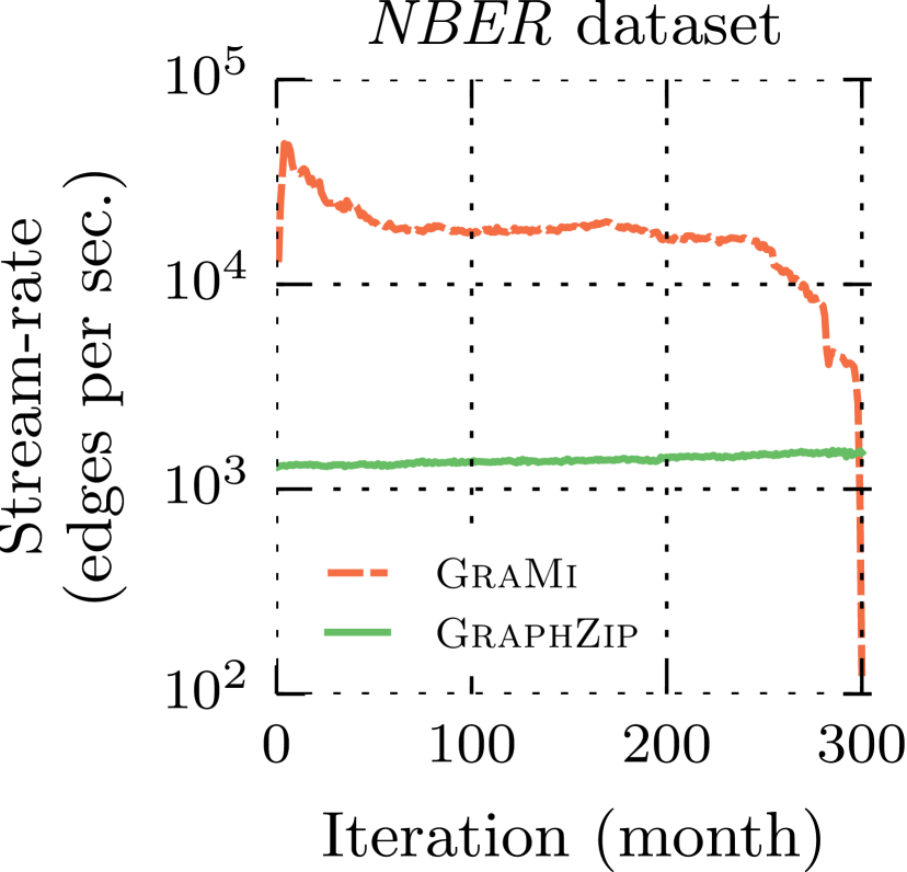
(a)

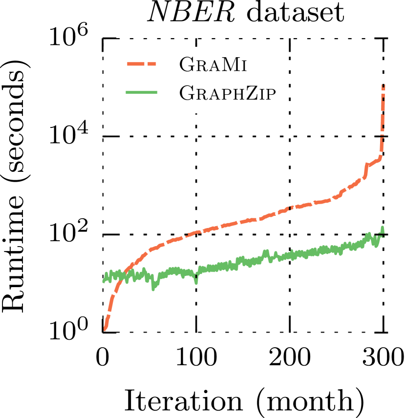
(b)

Figure 4. Stream-rate (a) and runtime (b) of GraphZip and GraMi on the NBER dataset. GraMi’s stream-rate decrease significantly near the end, while GraphZip’s stream-rate remains relatively constant.

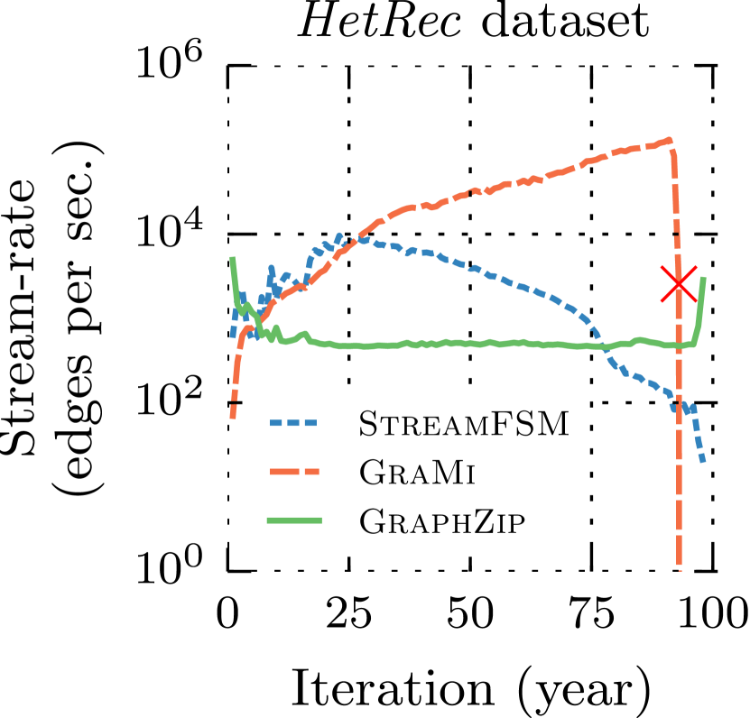
(a)

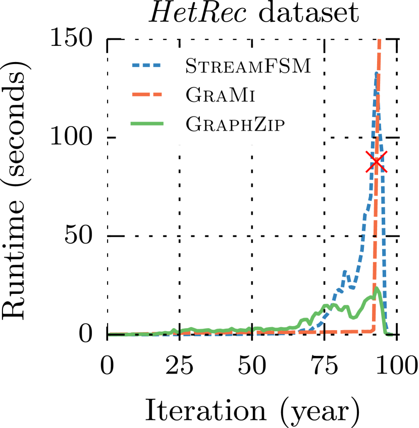
(b)

Figure 5. Stream-rate (a) and runtime (b) of GraphZip, GraMi, and StreamFSM on the HetRec dataset. Both GraMi and StreamFSM experience a massive spike in runtime near iteration 93.

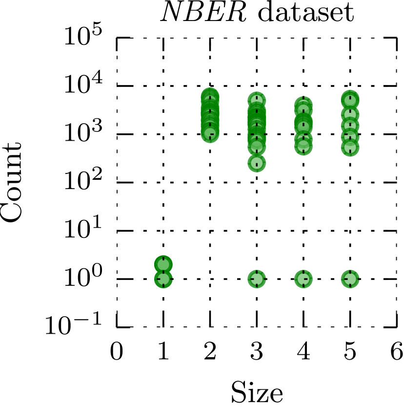
(a)

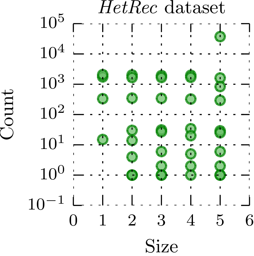
(b)

Figure 6. Distribution of GraphZip’s pattern dictionary after 300 iterations on NBER (a) and after 98 iterations on HetRec (b). The distribution for the larger NBER dataset (a) is skewed towards patterns with high frequencies, while the distribution for patterns in HetRec (b) is more varied.

4.4. Comparison with GraMi

Despite being designed for mining highly-compressing patterns like GraphZip, SUBDUE has clear performance issues that restrict benchmarking it against GraphZip on large real-world graphs. Therefore we also compare GraphZip with GraMi, a state-of-the-art graph mining system for frequent subgraph mining on large static graphs. In contrast to SUBDUE, GraMi is efficient enough to process datasets with millions of edges, however GraMi’s relative performance still allows us to motivate the need for graph mining algorithms designed explicitly to handle streaming data.

GraMi takes as input a single graph file as opposed to a sequence of edges, so in order to simulate mining a dynamic graph with a non-streaming method we append the previous graph with the next set of edges at each iteration, initializing the graph with the first set of edges. Thus, each iteration represents a ‘snapshot’ of the growing graph. Since both methods are paramaterized, we first tune GraMi’s minimum frequency threshold so that it returns a usable number of non-single edge patterns, then set GraphZip’s parameters (batch and dictionary size) such that the pattern dictionary resembles the set of subgraphs returned by GraMi. On NBER (figure 4), we fix GraMi’s minimum frequency threshold to 1000 which returned a set of subgraphs with a maximum, minimum, and average size of $6$, $1$, and $1.47$ respectively. Running GraphZip with $\alpha=5$ and $\theta=50$ resulted in a pattern dictionary with a maximum, minimum, and average subgraph size of $5$, $1$, and $2.89$ (figure 6 shows the dictionary distributions for both NBER and HetRec). Since the overall runtime of each model depends significantly on the configuration of the parameters, the main purpose of our comparison is to examine trends in the runtime and stream-rate of each model using settings where they return comparable sets of subgraphs.

Our results show that GraphZip is clearly more scalable than GraMi when mining large graphs in the streaming setting. While processing NBER, GraMi’s runtime (figure 4(b)) grows exponentially, experiencing a large spike near iteration 300. Figure 4(a) (normalized by patents per month) demonstrates this clearly: GraphZip maintains a constant stream-rate throughout, while GraMi’s stream-rate gradually slows until it sharply drops near the final updates. In fact, GraphZip’s stream-rate shows a slight increase over time; one explanation is that as the captured patterns in $P$ become more complex, less isomorphism checks occur per batch.

Results on the HetRec dataset indicate similar trends, though to a more extreme degree. With HetRec, we use a minimum frequency threshold of 9,000 for GraMi and keep the previous settings for GraphZip: setting the threshold to 1,000 causes GraMi’s stream-rate to slow to a relative crawl, and when using 10,000, GraMi is able to process the entire dataset but only returns two frequent subgraphs. While processing HetRec with the threshold set to 9,000, GraMi maintains a high stream-rate which trends upwards over time until the 93rd iteration, where the system freezes and is unable to make any progress despite being left running for multiple days (as indicated by the red ‘X’ on figures 5(a) and 5(b)).

4.5. Comparison with StreamFSM

Since there are no algorithms for mining highly-compressing subgraphs from graph streams in the existing literature, we benchmark GraphZip against StreamFSM, a recently developed streaming algorithm for frequent subgraph mining. Subgraphs that compress well are often both frequent and large, so the tasks of mining highly-compressing and frequently-occurring subgraphs are closely related. The StreamFSM reference implementation available online was unable to find any frequently occurring subgraphs with any large datasets other than the provided HetRec dataset (we hypothesize this is likely due to an implementation error), so we report results for StreamFSM on the HetRec dataset only.

A reasonable amount of time in the streaming setting equates to processing time less than or equal (at the very most) to the streaming-rate of the data; if the system cannot process the stream at the speed it is being generated, then the system is much less applicable in the real-life setting. Our results indicate that GraphZip is significantly more scalable than StreamFSM: while StreamFSM’s stream-rate experiences an initial speedup, it quickly and consistently deteriorates after iteration 25, drastically increasing the runtime per iteration. The severe increase in runtime occurs around the same iteration that GraMi freezes (see figure 5(b)). In contrast, GraphZip is seemingly unaffected by the same updates that cause massive slowdowns in GraMi and StreamFSM. GraphZip’s stream-rate becomes relatively constant after an initial slowdown, and remains constant through to the end of the experiment (see figure 5(a)). In the case of GraphZip and StreamFSM, the stream-rate of both systems is much faster than the average stream-rate of the data ($7.8\times 10^{-5}$ edges per second), despite StreamFSM’s relative volatility. However, a constant stream-rate is crucial for a deployed system processing a graph in real-time, since constraints on data processing time require predictable performance.

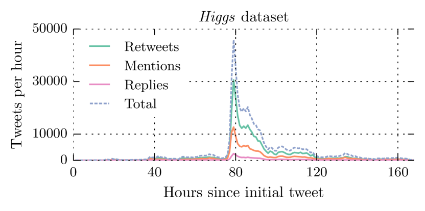
(a) Tracking Tweets per hour about the Higgs boson over time.

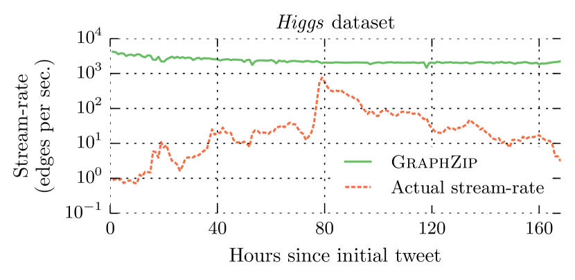
(b) Stream-rate of GraphZip on the Higgs dataset (higher is better).

Figure 7. (a) A large spike in activity occurs in the network after about 80 hours after the first Tweet. (b) After an initial slowdown, GraphZip converges to a constant stream-rate.

5. Twitter & the Higgs boson particle

One weakness of the datasets analyzed in the previous sections is the low granularity of their timestamps, e.g., HetRec can only be split into real-time streaming units as small as year, and the synthetic datasets have no time information at all. Streaming intervals (and therefore time between results) as long as a year are unlikely in a real deployment setting, especially when disk space is taken into consideration (storing a year’s worth of data before processing largely negates the benefit of streaming). For example, given a graph mining system configured to mine activity from a live network such as Twitter, it is likely that the user(s) would configure the interval to analyze patterns and trends over days, hours or even seconds. Additionally, reducing the time period between batches can reveal ebbs and flows in network activity that would be hidden by averaging out activity over a longer period.

The Higgs’s dataset has time data in seconds for each interaction, so we are able to pre-process the dataset into graph files segmented by the hour. One benefit to using the Higgs dataset is to observe how large spikes in network traffic affect the stream-rate; the minimum, maximum, and average number of edges streamed per hour are 43, 45,861, and 3,352 respectively, with the peak number of tweets per hour coinciding with the official announcement of the discovery.

As we can see in figure 7(b), GraphZip’s stream-rate is unaffected by the large spike in network traffic (using the same model parameters as the previous experiments). After an initial slowdown (similar to HetRec), GraphZip’s stream-rate converges on a constant stream-rate slightly faster than the maximum stream-rate the network reaches at the 80 hour mark, and much faster than the average stream-rate of the network ($9.3\times 10^{-1}$ tweets per second). Our results indicate that if GraphZip had been deployed to monitor the graph stream in real-time, it would have been able to process each set of updates before the next set of updates arrived.

6. Conclusion and Future Work

In this paper, we introduced GraphZip, a graph mining algorithm that utilizes a dictionary-based compression approach to mine highly-compressing subgraphs from a graph stream. We showed that GraphZip is able to successfully mine artificially-generated graphs for maximally-compressing patterns with comparable accuracy and much greater speed than a state-of-the-art approach. Additionally, we also demonstrated that GraphZip is able to surface both complex and insightful patterns from large real-world graphs at speeds much faster than the actual stream-rate, with performance exceeding that of openly available state-of-the-art non-streaming and streaming methods. Future work will focus on implementing the potential optimizations to the algorithm discussed in this paper, including approximation algorithms for (subgraph) isomorphism computations and naïve parallelization.

Appendix A Complexity Analysis

In this section we examine the time complexity of algorithm 1 in detail. We begin by analyzing the runtime per batch $B$ from a stream of graph $G$. Given a batch $B$, for each pattern $P^{(i)}\in P$ we retrieve the set $M$ of all embeddings (subgraph isomorphisms) of $P^{(i)}$ in $B$:

(5) $$\mathcal{O}(|P|\times\mathcal{O}(SI(P^{(i)},B)))$$

Then, for each embedding $M^{(i)}\in M$, we (a) extend a copy of $M^{(i)}$ by one edge length in each direction and (b) add the new pattern to the dictionary:

(6) $$\mathcal{O}( |P|\times(\mathcal{O}(SI(P^{(i)},B))\ +$$

$$|M|\times(|V_{M^{(i)}}|\times k+|P|\times\mathcal{O}(I(M^{(i)^{\prime}},P^{(i)})))))$$

where $k$ is the number of edges incident of $v\in V_{B}$ shared with $u\in V_{M^{(i)}}$, and $M^{(i)^{\prime}}$ is the extended copy of $M^{(i)}$. Finally, we add the remaining edges in $B$ as single-edge patterns ($e$) to $P$:

(7) $$\mathcal{O}( |P|\times(\mathcal{O}(SI(P^{(i)},B))\ +$$

$$|M|\times(|E_{M^{(i)}}|\times k+|P|\times\mathcal{O}(I(M^{(i)^{\prime}},P^{(i)}))))\ +$$

$$|R|\times\mathcal{O}(I(e,P^{(i)})))$$

If we use the well-known VF2 algorithm to implement the subgraph and graph isomorphism functions, the time complexity for $SI(.)$ and $I(.)$ simplify to $\mathcal{O}(V^{2})$ in the best case and $\mathcal{O}(V!\times V)$ in the worst case, where $V$ is the maximum number of vertices between the two graphs. Recall that our model is parameterized by $\theta$ and $\alpha$ ($|P|$ and $|E_{B}|$ respectively), which directly bounds $k<|V_{B}|<2\alpha$, $|M|<2^{\alpha}$ (maximum number of possible subgraphs in $B$), $E_{M^{(i)}}<\alpha$, and $|R|<\alpha$. Substituting in the worst case using VF2, we get:

(8) $$\mathcal{O}( \theta\times(({(2\alpha)!\times 2\alpha)}\ +$$

$$2^{\alpha}\times(\alpha\times 2\alpha+\theta\times{((2\alpha)!\times 2\alpha)}))\ +$$

$$\alpha\times 2!\times 2)$$

Which simplifies to:

(9) $$\mathcal{O}( \theta\times\alpha!\times\alpha\ +$$

$$\theta\times(2^{\alpha}\times\alpha^{2}+2^{\alpha}\times\theta\times\alpha!\times\alpha)+$$

$$\theta\times\alpha)$$

And lastly:

(10) $$\mathcal{O}(\theta^{2}\times 2^{\alpha}\times\alpha!\times\alpha)\\ =\mathcal{O}(\theta^{2}\times\alpha!)$$

Since $\theta$ and $\alpha$ are provided as parameters (constants at run-time), eq. 10 theoretically collapses to constant time ($\mathcal{O}(1)$), meaning that the GraphZip algorithm scales linearly with the size of the overall graph. However, our complexity analysis illustrates an important trade-off in selecting the batch size and dictionary size, since too large a value for either parameter can exponentially increase the run-time per batch (increasing $\alpha$ is particularly costly).

Our theoretical complexity analysis reinforces our experimental findings: that subgraph isomorphism calculations (a known NP-complete problem) dwarf all other computations in the algorithm. A promising area of future work would be to incorporate existing approximation algorithms for the subgraph isomorphism problem to increase the efficiency of GraphZip.

- [1] C. C. Aggarwal, Y. Li, P. S. Yu, and R. Jin. On dense pattern mining in graph streams. PVLDB, 3(1):975–984, 2010.
- [2] C. C. Aggarwal and H. Wang, editors. Managing and Mining Graph Data, volume 40 of Advances in Database Systems. Springer, 2010.
- [3] C. C. Aggarwal, Y. Zhao, and P. S. Yu. Outlier detection in graph streams. In ICDE, pages 399–409. IEEE Computer Society, 2011.
- [4] R. Agrawal and R. Srikant. Fast algorithms for mining association rules in large databases. In VLDB, pages 487–499. Morgan Kaufmann, 1994.
- [5] C. Avery. Giraph: Large-scale graph processing infrastructure on hadoop. Proceedings of the Hadoop Summit. Santa Clara, 11, 2011.
- [6] M. Berlingerio, F. Bonchi, B. Bringmann, and A. Gionis. Mining graph evolution rules. In ECML/PKDD, pages 115–130. Springer, 2009.
- [7] P. Braun, J. J. Cameron, A. Cuzzocrea, F. Jiang, and C. K. Leung. Effectively and efficiently mining frequent patterns from dense graph streams on disk. Procedia Computer Science, 35:338–347, 2014.
- [8] C. Bron and J. Kerbosch. Finding all cliques of an undirected graph (algorithm 457). Commun. ACM, 16(9):575–576, 1973.
- [9] I. Cantador, P. Brusilovsky, and T. Kuflik. Second workshop on information heterogeneity and fusion in recommender systems (hetrec2011). In RecSys, pages 387–388. ACM, 2011.
- [10] A. Ching, S. Edunov, M. Kabiljo, D. Logothetis, and S. Muthukrishnan. One trillion edges: Graph processing at facebook-scale. PVLDB, 8(12):1804–1815, 2015.
- [11] D. J. Cook and L. B. Holder. Substructure discovery using minimum description length and background knowledge. J. Artif. Intell. Res. (JAIR), 1:231–255, 1994.
- [12] D. J. Cook and L. B. Holder. Graph-based data mining. IEEE Intelligent Systems, 15(2):32–41, 2000.
- [13] D. J. Cook, L. B. Holder, and S. Djoko. Knowledge discovery from structural data. J. Intell. Inf. Syst., 5(3):229–248, 1995.
- [14] G. Cormode and S. Muthukrishnan. An improved data stream summary: the count-min sketch and its applications. J. Algorithms, 55(1):58–75, 2005.
- [15] M. De Domenico, A. Lima, P. Mougel, and M. Musolesi. The anatomy of a scientific rumor. (Nature Open Access) Scientific Reports, 3, 2013.
- [16] M. Elseidy, E. Abdelhamid, S. Skiadopoulos, and P. Kalnis. GRAMI: frequent subgraph and pattern mining in a single large graph. PVLDB, 7(7):517–528, 2014.
- [17] M. R. Garey and D. S. Johnson. Computers and intractability, volume 29. WH Freeman New York, 2002.
- [18] S. Ghazizadeh and S. S. Chawathe. Seus: Structure extraction using summaries. In Discovery Science, volume 2534 of Lecture Notes in Computer Science, pages 71–85. Springer, 2002.
- [19] B. H. Hall, A. B. Jaffe, and M. Trajtenberg. The NBER patent citation data file: Lessons, insights and methodological tools. Technical report, National Bureau of Economic Research, 2001.
- [20] L. B. Holder, D. J. Cook, and S. Djoko. Substucture discovery in the SUBDUE system. In KDD Workshop, pages 169–180. AAAI Press, 1994.
- [21] M. Kuramochi and G. Karypis. Frequent subgraph discovery. In ICDM, pages 313–320. IEEE Computer Society, 2001.
- [22] M. Kuramochi and G. Karypis. GREW-A scalable frequent subgraph discovery algorithm. In ICDM, pages 439–442. IEEE Computer Society, 2004.
- [23] M. Kuramochi and G. Karypis. Finding frequent patterns in a large sparse graph. Data Min. Knowl. Discov., 11(3):243–271, 2005.
- [24] J. Leskovec, J. M. Kleinberg, and C. Faloutsos. Graphs over time: densification laws, shrinking diameters and possible explanations. In KDD, pages 177–187. ACM, 2005.
- [25] A. McGregor. Graph stream algorithms: a survey. SIGMOD Record, 43(1):9–20, 2014.
- [26] N. Przulj. Biological network comparison using graphlet degree distribution. Bioinformatics, 26(6):853–854, 2010.
- [27] Y. Qian and K. Zhang. Graphzip: a fast and automatic compression method for spatial data clustering. In SAC, pages 571–575. ACM, 2004.
- [28] S. Ranu and A. K. Singh. Graphsig: A scalable approach to mining significant subgraphs in large graph databases. In ICDE, pages 844–855. IEEE Computer Society, 2009.
- [29] A. Ray, L. B. Holder, and S. Choudhury. Frequent subgraph discovery in large attributed streaming graphs. In BigMine, volume 36 of JMLR Workshop and Conference Proceedings, pages 166–181. JMLR.org, 2014.
- [30] J. Rissanen. Sochastic Complexity in Statistical Inquiry. Singapore: World Scientific Publishing, 1989.
- [31] J. Sun, C. Faloutsos, S. Papadimitriou, and P. S. Yu. Graphscope: parameter-free mining of large time-evolving graphs. In KDD, pages 687–696. ACM, 2007.
- [32] N. Tang, Q. Chen, and P. Mitra. Graph stream summarization: From big bang to big crunch. In SIGMOD Conference, pages 1481–1496. ACM, 2016.
- [33] C. H. C. Teixeira, A. J. Fonseca, M. Serafini, G. Siganos, M. J. Zaki, and A. Aboulnaga. Arabesque: a system for distributed graph mining. In SOSP, pages 425–440. ACM, 2015.
- [34] L. T. Thomas, S. R. Valluri, and K. Karlapalem. MARGIN: maximal frequent subgraph mining. volume 4, pages 10:1–10:42, 2010.
- [35] C. E. Tsourakakis, U. Kang, G. L. Miller, and C. Faloutsos. DOULION: counting triangles in massive graphs with a coin. In KDD, pages 837–846. ACM, 2009.
- [36] B. Wackersreuther, P. Wackersreuther, A. Oswald, C. Böhm, and K. M. Borgwardt. Frequent subgraph discovery in dynamic networks. In Proceedings of the Eighth Workshop on Mining and Learning with Graphs, pages 155–162. ACM, 2010.
- [37] X. Yan, H. Cheng, J. Han, and P. S. Yu. Mining significant graph patterns by leap search. In SIGMOD Conference, pages 433–444. ACM, 2008.
- [38] X. Yan and J. Han. gspan: Graph-based substructure pattern mining. In ICDM, pages 721–724. IEEE Computer Society, 2002.
- [39] X. Yan and J. Han. Closegraph: mining closed frequent graph patterns. In KDD, pages 286–295. ACM, 2003.
- [40] W. Yu, C. C. Aggarwal, S. Ma, and H. Wang. On anomalous hotspot discovery in graph streams. In ICDM, pages 1271–1276. IEEE Computer Society, 2013.
- [41] P. Zhao, C. C. Aggarwal, and G. He. Link prediction in graph streams. In ICDE, pages 553–564. IEEE Computer Society, 2016.
- [42] P. Zhao, C. C. Aggarwal, and M. Wang. gsketch: On query estimation in graph streams. PVLDB, 5(3):193–204, 2011.
- [43] J. Ziv and A. Lempel. Compression of individual sequences via variable-rate coding. IEEE Trans. Information Theory, 24(5):530–536, 1978.